Green’s function approach for quantum graphs: an overview

Abstract

Here we review the many aspects and distinct phenomena associated to quantum dynamics on general graph structures. For so, we discuss such class of systems under the energy domain Green’s function ($G$) framework. This approach is particularly interesting because $G$ can be written as a sum over classical-like paths, where local quantum effects are taking into account through the scattering matrix amplitudes (basically, transmission and reflection amplitudes) defined on each one of the graph vertices. Hence, the exact $G$ has the functional form of a generalized semiclassical formula, which through different calculation techniques (addressed in details here) always can be cast into a closed analytic expression. It allows to solve exactly arbitrary large (although finite) graphs in a recursive and fast way. Using the Green’s function method, we survey many properties for open and closed quantum graphs as scattering solutions for the former and eigenspectrum and eigenstates for the latter, also considering quasi-bound states. Concrete examples, like cube, binary trees and Sierpiński-like topologies are presented. Along the work, possible distinct applications using the Green’s function methods for quantum graphs are outlined.

1 Introduction

A graph can be understood intuitively as a set of elements (the vertices), attached ones to the others through connections (the edges). The topological arrangement of a graph is thus completely determined by the way the vertices are joined by the edges. The more general concept of a network – essentially a graph – has found applications in many branches of science and engineering. Some representative examples include: the analysis of electrical circuits, verification (in different contexts) of the shortest paths in grid structures, traffic planning, charge transport in complex chemical compounds, ecological webs, cybernetics architectures, linguistic families, and social connection relations, to cite just a few. In fact, given that as diverse as the street system of a city, the web of neurons in the human brain, and the organization of digital database in distinct storage devices, can all be described as ‘graphs’, we might be lead to conclude that such idea is one of the most useful and broadly used abstract mathematical notion in our everyday lives.

Less familiar is which we call quantum graphs, or more precisely quantum metric graphs (by associating lengths to the edges), basically comprising the study of the Helmholtz operator $\nabla^{2}+k^{2}$ – when the external potentials for the underlying Hamiltonian along the edges are null, see later – on these topological structures. Nevertheless, they still attract a lot of attention in the physics and mathematics specialized literature because their rich behavior and potential applications [1, 2], for instance, regarding wave propagation and diffusive properties (actually, this latter aspect allowing a possible formal association between the Schrödinger and the diffusion equations [3]).

Historically, Linus Pauling seems to be the first to foresee the usefulness of considering quantum dynamics on graph structures, e.g., to model free electrons in organic molecules [4, 5, 6, 7, 8, 9, 10]. Indeed, in a first approximation the molecules can be viewed as a set of fixed atoms (vertices) connected by chemical bonds (edges), along which the electrons obey a 1D Schrödinger equation with an effective potential. Moreover, quantum transport in multiply connected systems [11], like electron transport in organic molecules [12] as proteins and polymers, may be described by one-dimensional pathways (trajectories through the edges), changing from one path to another due to scattering at the vertices centers. More recently, quantum graphs have also been used to characterize molecular connectivity [13, 14].

In the realm of condensed matter physics, under certain conditions [15, 16] charge transport in solids is likewise well described by one-dimensional dynamics in branched (so network-like) structures, as in polymer films [17, 18]. Quantum graphs have also been applied in the analysis of disordered superconductors [19], Anderson transition in disordered wires [20, 21], quantum Hall systems [22], superlattices [23], quantum wires [24], mesoscopic quantum systems [25, 26, 27, 28], and in connection with laser tomography technologies [29].

To understand fundamental aspects of quantum mechanics, graphs are idealized exactly soluble models to address, e.g., band spectrum properties of lattices [30, 31], the relation between periodic-orbit theory and Anderson localization [32], general scattering [33], chaotic and diffusive scattering [34, 35, 36], and quantum chaos [37]. In particular, quantum graphs relevance in grasping distinct features of quantum chaotic dynamics have been demonstrated in two pioneer papers [38, 39]. Through elucidating examples, such works show that the corresponding spectral statistics follow very closely the predictions of the random-matrix theory [40]. They also present an alternative derivation of the trace formula, highlighting the similarities with the famous Gutzwiller’s expression for chaotic Hamiltonian systems [42, 41]. Actually, a very welcome fact in the area is the possibility to obtain exact analytic results for quantum graphs even when they present chaotic behavior [43, 44, 45, 46]. Important advances and distinct approaches to spectrum statistics analysis in quantum graphs, as well as the relation with quantum chaos, can be found in a nice review in [47].

As a final illustration of the vast applicability of graphs we mention two issues in the important fields of quantum information and quantum computing [48]. First, for the metric case (the focus in this review), it has been proposed that the logic gates necessary to process and operate qubits could be implemented by tailoring the scattering properties of the vertices along a quantum graph [49, 50]. However, much more common in quantum information is to consider only the topological features of the graphs [51], hence not ascribing lengths to the edges. Such structures are usually referred as discrete or combinatorial graphs (for a parallel between metric and combinatorial see, e.g., [52]). They are the basis to construct the so called graph-states [53, 54, 55, 56, 57], in which the vertices are the states themselves (e.g., spins 1/2 constituting the qubits) and the edges represent the pairwise interactions (for instance, an Ising-like coupling [58]) between two vertices states [59]. Graph-states are very powerful tools to unveil different aspects of quantum computation. For instance, to establish relations between different computational methods schemes [60, 57] and to demonstrate that entanglement can help to outperform the Shannon limit capacity (of the classical case) in transmitting a message with zero probability of error throughout a channel presenting noise [61, 62].

Second, also relevant in quantum information processing is the concept of quantum walks, loosely speaking, the quantum version of classical random walks [63, 64, 65]. Quantum walks are extremely useful either theoretically, as primitives of universal quantum computers [66, 67, 68], or operationally, as building blocks to quantum algorithms [69, 65, 70, 71]. Thus, since there is a close connection between quantum walks and quantum graphs [72, 73, 74, 75], this might open the possibility of extending different techniques to treat quantum graphs to the study of quantum walks [76, 77, 78, 79], therefore helping in the development of quantum algorithms.

The physical construction of quantum graphs is obviously an essential matter. In such regard, an important result is that in Ref. [80]. It shows that quantum graphs can be implemented through microwave networks due to the formal equivalence between the Schrödinger equation (describing the former) and the telegraph equation (describing the latter) [80]. Currently, these kind of systems are among the most preeminent experimental realizations of quantum graphs – as demonstrated by the vast literature on the topic [81, 82, 83, 84, 85, 86, 87, 88, 89, 90, 91, 92, 93, 94, 95, 96, 97, 98, 99, 100, 101]. Nonetheless, microwave networks are not the only possibility. In particular, optical lattices [102, 103, 104] and quasi-1D structures of large donor-acceptor molecules (with quasi-linear optical responses) [105] might also constitute very appropriate setups for building quantum graphs.

The implementation of quantum graphs – of course, alongside with the concrete applications – can also be quite helpful in settling relevant theoretical questions. As an illustrative example, consider the famous query posed by Mark Kac in 1966: ‘can one hear the shape of a drum?’ [106]. Its modified version in the present context is [107]: ‘can one hear the shape of a graph?’. It has been proved that for simple graphs (see next Sec.) whose all edges lengths are incommensurable, the spectrum is uniquely determined [107]. In other words, in this case one should be able to reconstruct the graph just from its eigenmodes. But if these assumptions are not verified, then distinct graphs can be isospectral [108, 109]. An interesting perspective to the problem arises by adding infinity leads to originally closed graphs [110, 111]. So, we have scattering system which can be analyzed in terms of their scattering matrices ${\mathcal{S}}$. Two metric graphs, ${\Gamma}_{A}$ and ${\Gamma}_{B}$, are said isoscattering either if ${\mathcal{S}}_{A}$ and ${\mathcal{S}}_{B}$ share the same set of poles or the phases of $\det[{\mathcal{S}}_{A}]$ and $\det[{\mathcal{S}}_{B}]$ are equal [112]. Hence, the question is now: can the poles of ${\mathcal{S}}$ and phases of $\det[{\mathcal{S}}]$ alone define the graph’s shape? The answer is again negative [110, 88], as nicely confirmed through microwave networks experiments [88] (see also [82]). However, by analyzing in more details actual scattering data (e.g., in the time instead of frequency domain [84]) it does become possible to distinguish isoscattering graphs which are topologically different.

Quantum graphs as a well posed general mathematical problem requires the establishment of the underlying self-adjoint operator, i.e., the proper definition of the wave equation with its correct boundary conditions. Probably, the first important step along this direction was taken in 1953 in Ref. [7]. There, graphs were thought of as idealized web of wires or wave guides, but for the widths being much smaller than any other spatial scale. Assuming the lateral size of the wire small enough, any propagating wave remains in a single transverse mode. Therefore, instead of the corresponding partial differential Schrödinger equation, one can deal with ordinary differential operators. If no external field is applied or no potential $V$ for the wires is assumed, the one dimensional motion along the edges is free and anywhere in the graph the wave number reads $k=\sqrt{2\mu E/\hbar^{2}}$, with the energy $E$ a constant. Concerning the nodes, they either can be faced as scattering centers (thus, conceivably described by local ${\mathcal{S}}$ matrices) or the loci where consistent matching conditions for the partial wave functions (i.e., the $\psi$’s in the distinct edges) must be imposed (Sec. 2).

In contrast, graphs with non-vanishing potentials – sometimes referred to as ‘dressed’ [113, 44] – lead to solutions with spatially dependent $k$’s along the edges. An important subset of dressed are scaling quantum graphs [114, 115, 116, 44, 43, 117], whose mathematical foundations are discussed in [118]. They are particularly interesting because although their classical limit is chaotic, the quantum spectrum is exactly obtained through analytic periodic orbit expansions [43]. Another very relevant class of dressed quantum graphs is that described by magnetic Schrödinger operators [119]. In this case one assumes arbitrary inhomogeneous magnetic fields in the network [120], such that for each edge $e$ there is a corresponding vector potential $A_{e}$. So, formally we have to make the traditional momentum operator substitution in the Schrödinger equation: $d/dx_{e}\rightarrow d/dx_{e}-iA_{e}$. Recently, quantum graphs with magnetic flux have attracted a lot of attention due to the many distinct phenomena emerging in these systems [121, 122, 123, 124, 125, 126, 127, 128].

Given the discussion so far, it is already clear that a quantum graph is, after all, just an usual quantum problem. As such, its solution basically means to determine properties like wave packets propagation [129, 130], eigenstates (either bound and scattering states) [131, 132], eigenenergies [133], etc. This can be accomplished from, say, a suitable Schrödinger equation and appropriate boundary conditions for each specific graph topology, Sec. 2. But operationally there are many ways to mathematically deal with these systems, so different techniques can be employed. For instance, we can cite self-adjoint extension approaches [134], and the previously mentioned scattering ${\mathcal{S}}$ matrix methods [38] and the trace formula based on classical periodic orbits expansions [39].

It is well known that the energy Green’s function $G$ is a very powerful tool in quantum mechanics [135, 136]. Its knowledge allows to determine essentially any relevant quantity for the problem (e.g., the time evolution can be calculated from the time-dependent propagator, which is the Fourier transform of $G$). So, it should be quite natural to consider Green’s function approaches in the study of graph structures. In fact, one of the first works in this direction [35] has employed $G$ to describe transport in open graphs. Later, the many possibilities in utilizing Green’s functions techniques for arbitrary quantum graphs have been discussed and exemplified in [137], with general and rigorous results further obtained from such a method in [138, 139]. Recently, Green’s functions have been used to investigate (always in the context of quantum graphs): searching algorithms for shortest paths [140], Casimir effects [141], vacuum energy in quantum field theories [142], and resonances on unbounded star-shaped networks [143]. Lastly, but not the least important, the special topological features of networks make it possible (at least in the undressed case) to obtain the exact $G$ in a closed analytic form for any finite (i.e., a large although limited number of nodes and edges) arbitrary graph. Certainly, this contrasts with most problems in quantum mechanics, for which exact analytic solutions are very hard to find [144, 145].

Therefore, regarding the purpose of this review, we start observing there is a huge literature discussing general features and applications of classical graphs. To cite just one, more physics-oriented, we mention communicability – so, signal transport – in classical networks [146]. In the quantum case comprehensive overviews are not so abundant, notwithstanding particular relevant aspects can be found addressed in details in some very interesting works [39, 47, 1, 147, 52, 148] (with also a good source of a formal and rigorous treatment being [149]). In this way, our first goal is to survey graphs as ordinary quantum mechanics problems, but highlighting that their special characteristics can give rise to rich quantum phenomena.

The second is to do so by specifically considering one of the most powerful methods to treat quantum graphs, namely, the Green’s function approach. For arbitrary graphs, we discuss in an unified manner how to obtain the exact energy domain $G$ as a general sum over paths ‘a la Feynman’ [150, 151, 152]. These paths must be weighted by the proper quantum amplitudes, given by energy-dependent scattering matrices elements associated to the vertices. We examine a schematic way to regroup the multi-scattering contributions (essentially a factorization method [134, 153, 154, 155]), leading to a final closed analytic expression for $G$. This particular procedure to construct the exact $G$ is very useful to interpret many results concerning quantum graphs, like interference in transport processes [35, 156, 157]. With the help of illustrative examples, we elaborate on how to extract from $G$ the graphs quantum properties.

The work is organized as the following. In Section 2 we define and discuss general quantum graphs. In Section 3 we consider in great detail the Green’s function approach for such systems. In Section 4 we present (with examples) the factorization protocols which allow to cast $G$ as a closed analytic formula. Distinct applications are addressed in the next three Sections. More specifically, the general determination of bound and scattering states, analysis of representative graphs (cube, binary trees, and Sierpiński-like graphs), and quasi-bound states in open structures, are considered, respectively, in Secs. 5, 6, and 7. Finally, we drawn our final remarks and conclusion in Section 8.

2 Quantum mechanics on graphs: general aspects

2.1 Graphs

A finite graph $X(V,E)$ is a pair consisting of two sets, of vertices (or nodes) $V(X)=\{1,2,\ldots,n\}$ and of edges (or bonds) $E(X)=\{e_{1},e_{2},\ldots,e_{m}\}$ [158, 159]. Thus, the total number of vertices and edges is given, respectively, by $n=|V(X)|$ and $m=|E(X)|$. If the vertices $i$ and $j$ are linked by the edge $e_{s}$, then $e_{s}\equiv\{i,j\}$ (hereafter $i,j=1,\ldots,n$ and $r,s=1,\ldots,m$). For an undirected graph, any edge $\{i,j\}$ has the same properties [160] in both $i\rightarrow j$ and $j\rightarrow i$ ‘directions’: $\{i,j\}\equiv\{j,i\}$. For simple graphs $e_{s}\neq\{j,j\}$ and $e_{r}=e_{s}$ only if $r=s$. Hence, in this case there are no loops or pair of vertices multiple-connected. Finally, for connected graphs the vertices cannot be divided into two non-empty subsets such that there is no edge joining the two subsets.

The graph topology, i.e., the way the vertices and edges are associated, can be described in terms of the adjacency matrix $A(X)$ of dimension $n\times n$. For simple undirected graphs, the $ij$-th entry of $A(X)$ reads

$$A_{ij}(X)=\begin{cases}1,&\;\text{\rm if }\;\{i,j\}\in E(X),\\ 0,&\;\text{\rm otherwise}.\end{cases}$$ (1)

Two vertices are said neighbors whenever they are connected by an edge. Thus, the set

$$E_{i}(X)=\left\{j:\{i,j\}\in E(X)\right\}$$ (2)

is the neighborhood of the vertex $i\in V(X)$ and the degree (or valence) of $i$ is

$$v_{i}=|E_{i}(X)|=\sum_{j=1}^{n}A_{ij}(X).$$ (3)

Note that

$$|E(X)|=\frac{1}{2}\sum_{i=1}^{n}|E_{i}(X)|.$$ (4)

So far, the above definitions refer to discrete or combinatorial graphs. To discuss quantum graphs it is necessary to equip the graphs with a metric. Therefore, a metric graph $\Gamma(V,E)$ is a graph $X(V,E)$ for which it is also assigned a length $\ell_{e_{s}}\in(0,+\infty)$ to each edge. If all edges have finite length the metric graph is called compact, otherwise it is non-compact. In this latter case $\Gamma$ has one ore more ‘leads’. A lead is a single ended edge $e_{r}$, which leaves from a vertex and extends to the semi-infinite (so $\ell_{e_{s}}=+\infty$).

In the quantum description, for each edge $e_{s}$ (with $e_{s}$ either joining two vertices $i$ and $j$ or leaving from vertex $j$ to the infinite) we assume a coordinate $x_{e_{s}}$, indicating the position along the edge. For $e_{s}=\{i,j\}$, to choose at which vertex ($i$ or $j$) $x_{e_{s}}=0$ and $x_{e_{s}}=\ell_{e_{s}}$ is just a matter of convention, and can be set according to the convenience in each specific system. Of course, for $e_{s}$ a lead attached to $j$, a natural choice is $x_{e_{s}}=0$ at $j$.

In the remaining of this review we will (mainly but not only) focus on simple connected graphs, the most studied situation in quantum mechanics [73]. But we stress that the Green’s function discussed here is also valid for non-simple graphs, i.e., for many edges joining the same two vertices and for the existence of loops: one just need to consider the proper reflections and transmissions quantum amplitudes (Sec. 3) for the propagation along these extra edges. This will be illustrated with certain examples in Sec. 6.

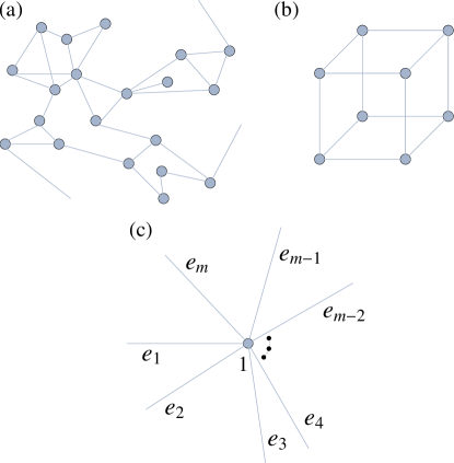
Figure 1: (Color online). Examples of (a) open and (b) closed quantum graphs. (c) A open star graph with a single vertex $V(\Gamma)=\{1\}$ connected to $E(\Gamma)=\{e_{1},\ldots,e_{m}\}$ leads.

2.2 The time-independent Schrödinger equation on graphs

A quantum graph is a metric graph structure $\Gamma(V,E)$, on which we can define a differential operator $H$ (usually the Schrödinger Hamiltonian) together with proper vertices boundary conditions [39, 47]. In others words, a quantum graph problem is a triple

$$\{\text{$\Gamma(V,E)$, Hamiltonian operator $H$ on $E(\Gamma)$, boundary conditions for $V(\Gamma)$}\}.$$

A quantum graph is called closed if the respective metric graph is compact, otherwise it is called open. A schematic representation of quantum graphs [160] is depicted in Figure 1.

The total wave function $\Psi$ is a vector with $m$ components, written as

$$\Psi=\left(\begin{array}[]{c}\psi_{e_{1}}(x_{e_{1}})\\ \psi_{e_{2}}(x_{e_{2}})\\ \vdots\\ \psi_{{e_{m}}}(x_{e_{m}})\end{array}\right).$$ (5)

The Hamiltonian operator on $E(\Gamma)$ consists of the following unidimensional differential operators defined on each edge $e_{s}$ [161, 19] (the dressed case)

$$H_{e_{s}}(x_{e_{s}})=-\frac{\hbar^{2}}{2\mu}\frac{d^{2}}{dx_{e_{s}}^{2}}+V_{e_{s}}(x_{e_{s}}).$$ (6)

Here, $V_{e_{s}}(x_{e_{s}})$ is the potential (usually assumed to be non-negative and smooth) in the interval $0<x_{e_{s}}<\ell_{e_{s}}$. Different works have considered the above Hamiltonian for non-vanishing potentials (for instance, see [116, 44, 43, 137, 162, 163, 164, 165]). However, in the literature, even in papers discussing quantum chaos [38, 39, 47, 166, 37], it is usual to have for any $e_{s}$ that $V_{e_{s}}=0$ (the case we assume in this review). Then, the component $\psi_{e_{s}}(x_{e_{s}})$ of the total wave function $\Psi$ is the solution of ($k=\sqrt{2\mu E}/\hbar$)

$$-\frac{d^{2}\psi_{e_{s}}}{dx_{e_{s}}^{2}}=k^{2}\psi_{e_{s}}(x_{e_{s}})\ \Rightarrow\ \psi_{e_{s}}(x_{{e}_{s}})=c_{+,e_{s}}\,\exp[+i\,k\,x_{e_{s}}]+c_{-,e_{s}}\,\exp[-i\,k\,x_{e_{s}}],$$ (7)

with the $c$’s constants. All these wave functions must satisfy appropriate boundary conditions at the vertices, ensuring continuity, global probability current conservation, divergence free $\psi$’s and uniqueness. Technically, the match of the boundary conditions in each vertex is the most cumbersome step in obtaining the final full $\Psi$ (in Figure 2 we illustrate which components must be matched in which vertices for a particular example of a graph with $V(\Gamma)=\{1,2,3,4,5\}$ and $E(\Gamma)=\{\{1,2\},\{2,3\},\{3,4\},\{3,5\}\}$).

Furthermore, the imposition of these boundary conditions [39, 47, 167] renders the Hamiltonian operator to be self-adjoint . In fact, the most general boundary conditions at a vertex of a quantum graph (consistent with flux conservation [30]) can be determined through self-adjoint extension techniques [168, 169]. Let us denote by [134, 153] ${\Psi_{j}}=(\psi_{e_{j_{1}}},\psi_{e_{j_{2}}},\ldots,\psi_{e_{j_{v_{j}}}})^{T}$ and ${\Psi_{j}^{\prime}}=(\psi_{e_{j_{1}}}^{\prime},\psi_{e_{j_{2}}}^{\prime},\ldots,\psi_{e_{j_{v_{j}}}}^{\prime})^{T}$, respectively, the wave functions and their derivatives associated to the $v_{j}$ edges attached to the vertex $j$. Then, the boundary conditions can be specified through $v_{j}\times v_{j}$ matrices ${\mathcal{A}}_{j}$ and ${\mathcal{B}}_{j}$, with ${\mathcal{A}}_{j}\Psi_{j}={\mathcal{B}}_{j}\Psi_{j}^{{}^{\prime}}$ at $j$. One ensures self-adjointeness of the Hamiltonian operator by imposing current conservation $\Psi_{j}^{\dagger}\Psi_{j}^{\prime}={\Psi^{\prime}}_{j}^{\dagger}\Psi_{j}$. As shown in [134, 153], the general solution for this problem implies that ${\mathcal{A}}_{j}{\mathcal{B}}_{j}^{\dagger}={\mathcal{B}}_{j}{\mathcal{A}}_{j}^{\dagger}$, resulting in a set of $v_{j}^{2}$ independent real parameters to characterize the boundary conditions at $j$. More on this is discussed in the Appendix A, but here we comment that in physical terms, the self-adjointness of the Hamiltonian implies that the dynamics does not allow the vertices to behave as sinks or sources.

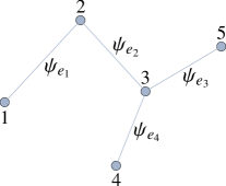
Figure 2: (Color online). A quantum graph $\Gamma(V,E)$ – with $V(\Gamma)=\{1,2,3,4,5\}$ and $E(\Gamma)=\{\{1,2\},\{2,3\},\{3,4\},\{3,5\}\}$ – and the indication of the $\psi_{e_{s}}$ components of $\Psi$ in each one of the $\Gamma$ edges. The wave functions must be matched through the boundary condition at each vertex $i\in V(\Gamma)$. Specifically: at $i=1$: $\psi_{e_{1}}$; at $i=2$: $\psi_{e_{1}},\psi_{e_{2}}$; at $i=3$: $\psi_{e_{2}},\psi_{e_{3}},\psi_{e_{4}}$; at $i=4$: $\psi_{e_{4}}$; at $i=5$: $\psi_{e_{3}}$.

2.3 The vertices as zero-range potentials

From the previous discussion, in an undressed quantum graph the edges $e_{s}$ can be viewed as free unidimensional spatial directions of length $\ell_{e_{s}}$ and the vertices as point structures (0D), whose action is to impose the proper boundary conditions on the $\psi$’s. In the usual 1D quantum mechanics, arbitrary zero-range potentials, also known as point interactions, have exactly such effect [170, 171] (see Appendix A.1). A textbook example is the Dirac delta-function potential that simply determines, at its location, a specific boundary condition to the wave function [172].

Hence, to describe the quantum dynamics along a graph we can take the $j$’s as arbitrary zero-range interactions, an approach fully consistent with the general boundary conditions treatment described in Sec. 2.2 (Appendix A). To assume the vertices as potentials brings up two important advantages. (a) The $j$’s become point scatterers, which are completely characterized by their reflections and transmission amplitudes (recall this is exactly the case for a delta-function, for which $\psi$ can be obtained without considering any boundary conditions). So, a purely scattering treatment solves the problem – see, e.g., the pedagogical discussion in [173]. (b) General point interactions are very diverse in their scattering properties. For instance, the intriguing aspects of transmission and reflection from point interactions have been discussed in distinct situations, such as, time-dependent potentials [174], nonlinear Schrödinger equation [175] and shredding by sparse barriers [176]. So, the mentioned procedure allows to have all the features of arbitrary zero-range potentials also in the context of quantum graphs.

As demonstrated in the Appendix A.1, to determine the boundary conditions that a point interaction in the line (say, at $x_{0}=0$) imposes on the the wave function at $x=0$ is entirely equivalent to specify the potential scattering ${\mathcal{S}}$ matrix elements. This also holds true when the vertex, a zero-range potential, instead of being attached to two edges (the ‘left’ ($-\infty<x<0$) and ‘right’ ($0<x<+\infty$) semi-infinite leads for the 1D line case), is connected to $v_{j}$ edges, representing $v_{j}$ 1D “directions”, see Figure 1 (c). From the Appendix A.2, we then can define for each vertex $j$ a matrix ${\mathcal{S}}_{j}$, of elements ${\mathcal{S}}_{j}^{(s,s)}(k)=r_{j}^{(s)}(k)$ and ${\mathcal{S}}_{j}^{(s,r)}(k)=t_{j}^{(s,r)}(k)$ (from now on, we will label edges $e_{j_{s}}$ and $e_{j_{r}}$ simply as $s$ and $r$), such that

• $t_{j}^{(s,r)}(k)$ is the quantum amplitude for a plane wave, of wave number $k$, incoming from the edge $r$ towards the vertex $j$ to be transmitted to the edge $s$ outgoing from $j$.

• $r_{j}^{(s)}(k)$ is the quantum amplitude for a plane wave, of wave number $k$, incoming from the edge $s$ towards the vertex $j$ to be reflected to the edge $s$ outgoing from $j$.

The required conditions for self-adjointeness (i.e., probability flux conservation) along the whole graph (Appendix A.3), demands that ${{\mathcal{S}}}(k){{\mathcal{S}}}^{\dagger}(k)={{\mathcal{S}}}^{\dagger}(k){{\mathcal{S}}}(k)=\mathbf{1}$ and ${{\mathcal{S}}}(k)={{\mathcal{S}}}^{\dagger}(-k)$, so yielding

$$\sum_{l=1}^{v_{j}}{\mathcal{S}}_{j}^{(s,l)}(k)\,{{\mathcal{S}}_{j}^{(r,l)}}^{*}(k)=\sum_{l=1}^{v_{j}}{\mathcal{S}}_{j}^{(l,s)}(k)\,{{\mathcal{S}}_{j}^{(l,r)}}^{*}(k)=\delta_{sr},\ \ \mathcal{S}_{j}^{(s,r)}(k)={{\mathcal{S}}_{j}^{(r,s)}}^{*}(-k).$$ (8)

Summarizing, for quantum graphs it is complete equivalent to set either the boundary conditions for the $\psi$’s at each vertex, as mentioned in Sec. 2.2, or to specify the scattering properties of the different $j$’s through the ${\mathcal{S}}_{j}^{(r,s)}$ matrices obeying to Eq. (8). We also observe that eventually one could have bound states for a given point interaction potential $j$ depending on the particular BC imposed to $\psi$ at the vertex location. In the scattering description, the quantum coefficients $R$ and $T$ have poles at the upper-half of the complex plane $k$, corresponding to the possible eigenenergies. The eigenfunctions can then be obtained from an appropriate extension of the scattering states to those $k$’s values [177]. This will be exemplified in Section 6.

3 Energy domain Green’s functions for quantum graphs

3.1 The basic Green’s function definition in 1D

The Green’s function $G(E)$ is an important tool in quantum mechanics [135]. In the usual 1D case, it is defined by the inhomogeneous differential equation ($H(x)=-(\hbar^{2}/(2\mu))\,d^{2}/dx^{2}+V(x)$)

$$[E-H(x_{f})]G(x_{f},x_{i};E)=\delta(x_{f}-x_{i}),$$ (9)

where $G(x_{f},x_{i};E)$ is also subjected to proper boundary conditions.

Suppose we have a complete set of normalized eigenstates $\psi_{s}(x)$ ($s=0,1,...$, discrete spectrum) and $\psi_{\sigma}(x)$ ($\sigma>0$, continuum spectrum), with

$$H\,\psi_{s}=E_{s}\,\psi_{s},\qquad H\,\psi_{\sigma}=\frac{\hbar^{2}\sigma^{2}}{2\mu}\,\psi_{\sigma}.$$ (10)

Then, the solution of Eq. (9) is formally

$$G(x_{f},x_{i};E)=\sum_{s}\frac{\psi_{s}(x_{f})\,{\psi_{s}}^{*}(x_{i})}{(E-E_{s})}+\int_{0}^{\infty}d\sigma\,\frac{\psi_{\sigma}(x_{f})\,{\psi_{\sigma}}^{*}(x_{i})}{(E-\hbar^{2}\sigma^{2}/(2\mu))}.$$ (11)

From Eq. (11) we can identify the poles of the Green’s function with the bound states eigenenergies $E_{s}$ and the residues at each pole with a tensorial product of the corresponding bound state eigenfunction. The continuous part of the spectrum corresponds to a branch cut of $G(x_{f},x_{i};E)$ [178, 179]. Given Eq. (11), the limit

$$\lim_{E\to E_{s}}(E-E_{s})\,G(x_{f},x_{i};E)=\psi_{s}(x_{f})\,{\psi_{s}}^{*}(x_{i})$$ (12)

can be used to extract the discrete bound states from $G$.

3.2 The exact Green’s function written as a generalized semiclassical expression

There are basically three methods for calculating the Green’s function [135]: solving the differential equation in (9); summing up the spectral representation in (11); or performing the Feynman path integral expansion for the propagator in the energy representation [180, 181]. In particular, for contexts similar to the present work (see next), the latter approach has been used to study scattering by multiple potentials in 1D [150, 151], to calculate the eigenvalues of multiple well potentials [152], to study scattering quantum walks [77, 78], and to construct exact Green’s function for piecewise constant potentials [182, 183].

The exact Green’s function for an arbitrary finite array of potentials of compact support has been obtained in [150], with an extension for more general cases presented in [151]. For the derivations in [150], it is necessary for the $r$’s and $t$’s of each localized potential to satisfy to certain conditions, which indeed are the ones in the Appendix A, Eq. (112) (note that point interactions constitute a particular class of potentials of compact support [184]). Thus, based on [150] we can calculate the Green’s function for general point interactions by using the corresponding reflection and transmission coefficients, which are quantities with a very clear physical interpretation and conceivably amenable to experimental determination [185, 186].

So, for these general array of potentials, according to Refs. [150, 151, 152] the exact (hence in contrast with usual semiclassical approximations, see footnote 2) Green’s function for a fixed energy $E$ (and end points $x_{i}$ and $x_{f}$) is given by

$$G(x_{f},x_{i};E)=\frac{\mu}{i\hbar^{2}k}\sum_{\mbox{\scriptsize sp}}W_{\mbox{\scriptsize sp}}\exp{[\frac{i}{\hbar}S_{\mbox{\scriptsize sp}}(x_{f},x_{i};k)]}.$$ (13)

The above sum is performed over all scattering paths (sp) starting in $x_{i}$ and ending in $x_{f}$. A ‘scattering path’ represents a trajectory in which the particle leaves from $x_{i}$, suffers multiple scattering, and finally arrives at $x_{f}$. For each sp, $S_{\mbox{\scriptsize sp}}$ is the classical-like action, i.e., $S_{\mbox{\scriptsize sp}}=k\,L_{\mbox{\scriptsize sp}}$, with $L_{\mbox{\scriptsize sp}}$ the trajectory length. The term $W_{\mbox{\scriptsize sp}}$ is the sp quantum amplitude (or weight), constructed as the following: each time the particle hits a localized potential $V_{n}$, quantically it can be reflected or transmitted by the potential. In the first case, $W_{\mbox{\scriptsize sp}}$ gets a factor $r_{n}$ and in the second, $W_{\mbox{\scriptsize sp}}$ gets a factor $t_{n}$. The total $W_{\mbox{\scriptsize sp}}$ is then the product of all quantum coefficients $r_{n}$’s and $t_{n}$’s acquired along the sp.

The direct extension of Eq. (13) – often called generalized semiclassical Green’s function formula because its functional form – to quantum graphs is natural. In fact, the two main ingredients necessary in the rigorous derivation [150, 151] of Eq. (13), namely, unidimensionality and localized potentials, are by construction present in quantum graphs. First, since the quantum evolution takes place along the graph edges, regardless the graph topology, the dynamics is essentially 1D. Second, the potentials (scatters) are the vertices, which as we have seen, can be treated as point interactions, so a particular class of compact support potentials [187, 184].

In the Appendix B we outline the main steps necessary to prove that the exact Green’s function for arbitrary quantum graphs has the very same form of Eq. (13). Moreover, as we are going to discuss in length in Sec. 4, different techniques can be used to identify and sum up all the scattering paths. So, for general finite (i.e., $|V(\Gamma)|$ and $|E(\Gamma)|$ both finite) connected undirected simple metric quantum graphs $\Gamma$, in principle one always can obtain a closed analytical expression for $G$. Therefore, given that any information about a quantum system can be extracted directly from the corresponding Green’s function, the results here constitute a very powerful tool in the analysis of many distinct aspects of quantum graphs.

As a final observation, we recall that for scaling quantum graphs [118], for each edge $e_{s}$ we have $k_{e_{s}}=\gamma_{e_{s}}\,k_{0}$ (see footnote 3). But this behavior for the wave number also would result from constant potentials $V_{e_{s}}$ along the distinct $e_{s}$’s. Moreover, as discussed in [183], the correct $G$ for these kind of piecewise constant potential systems can too be cast as above. Therefore, the exact Green’s function for scaling quantum graphs are likewise given by Eq. (13).

4 Obtaining the Green’s function for quantum graphs: general procedures

The formula in Eq. (13) gives the correct Green’s function for arbitrary connected undirected simple quantum graphs. However, it has no universal practical utility unless we are able to generally identify all the possible scattering paths and to sum up the resulting infinite series regardless the specific system. So, here we shall describe different protocols to handle Eq. (13), allowing to write the exact $G$ as a closed analytic expression. To keep the discussion as accessible as possible, we start with few straightforward illustrative examples. In the sequence we extend the analysis to more complex situations.

We adopt the following notation:

• $r_{j}^{(s)}$ and $t_{j}^{(s,r)}$ are the reflection and transmission amplitudes for the vertex $j$, as described in the end of Sec. 2.

• $P_{l}$ represents the contribution from an entire infinite family $l$ of sp to Eq. (13), so that $G=\mu/(i\hbar^{2}k)\sum_{l}P_{l}$.

• $G_{sr}(x_{f},x_{i};k)$ is the Green’s function for a particle with energy $E={\hbar^{2}k^{2}}/{2\mu}$, whose initial point $x_{i}$ lies in the edge $e_{r}$ and the final point $x_{f}$ in the edge $e_{s}$.

Also, whenever there is no room for doubt, for simplicity we represent edges by $s$ (instead of $e_{s}$) and vertices by capital letters, $A$, $B$, etc.

4.1 Constructing the Green’s function: a simple example

Consider the open graph shown in Fig. 3 (a). It has two vertices, $A$ and $B$, one finite edge (of length $\ell_{1}$), labeled 1, and two semi-infinite edges (leads), labeled $i$ and $f$. By assuming $0\leq x_{i}<+\infty$ ($x_{i}=0$ at $A$) in $i$ and $0\leq x_{f}<+\infty$ ($x_{f}=0$ at $B$) in $f$, the Green’s function $G_{fi}(x_{f},x_{i};k)$ essentially describes the transmission across the full graph structure, i.e., from the left to the right leads. To obtain $G$ we need to sum up all the possible sp for a quantum particle starting at $x_{i}$, in $i$, going through multiple reflections between the vertices $A$ and $B$, and finally ending up at $x_{f}$, in $f$. As we shall demonstrate, Eq. (13) then yields a convergent geometric series, which therefore can be calculated exactly [188, 189, 190, 150, 151, 191, 192, 152, 193].

In Fig. 3 (b)–(d) it is depicted three examples of sp. Consider the scattering path in Fig. 3 (b), representing the ‘direct’ propagation from $x_{i}$ to $x_{f}$. The particle starts by leaving $x_{i}$ towards $A$. From this first stretch of the trajectory, one gets a factor $\exp[ikx_{i}]$ to $G$. Upon hitting the vertex, the particle is then transmitted through $A$. This process yields a factor $t_{A}^{(1,i)}$ to $G$. Next, the particle goes to the vertex $B$ location, leading to a factor $\exp[ik\ell_{1}]$. Once in $B$, the particle is then transmitted through $B$, thus resulting in $t_{B}^{(f,1)}$. Finally, from the final trajectory stretch ($B$ to $x_{f}$), one gets $\exp[ikx_{f}]$. Putting all this together, the sp of Fig. 3 (b) contributes to Eq. (13) with $W_{sp}=t_{A}^{(1,i)}\,t_{B}^{(f,1)}$ and $L_{sp}=(x_{f}+x_{i})+\ell_{1}$ (hence the length of this sp).

Following the same type of analysis, for the other two examples in Fig. 3 we have:

(c) $$\exp[ikx_{i}]\,t_{A}^{(1,i)}\,\exp[ik\ell_{1}]\,r_{B}^{(1)}\,\exp[ik\ell_{1}]\,r_{A}^{(1)}\,\exp[ik\ell_{1}]\,t_{B}^{(f,1)}\,\exp[ikx_{f}]:$$

$$W_{sp}=r_{A}^{(1)}\,r_{B}^{(1)}\,t_{A}^{(1,i)}\,t_{B}^{(f,1)},\qquad L_{sp}=(x_{f}+x_{i})+3\ell_{1};$$

(d) $$\exp[ikx_{i}]\,t_{A}^{(1,i)}\,\exp[ik\ell_{1}]\,r_{B}^{(1)}\,\exp[ik\ell_{1}]\,r_{A}^{(1)}\,\exp[ik\ell_{1}]\,r_{B}^{(1)}\,\exp[ik\ell_{1}]r_{A}^{(1)}\,\exp[ik\ell_{1}]\,t_{B}^{(f,1)}\,\exp[ikx_{f}]:$$

$$W_{sp}=(r_{A}^{(1)})^{2}\,(r_{B}^{(1)})^{2}\,t_{A}^{(1,i)}\,t_{B}^{(f,1)},\qquad L_{sp}=(x_{f}+x_{i})+5\ell_{1}.$$

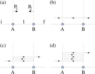
Figure 3: (Color online). A simple graph with two vertices, $A$ and $B$, a finite edge labeled 1 (of length $\ell_{1}$), and left, $i$, and right, $f$, leads. (a) The starting positions of two families, $P_{1}$ and $P_{2}$, of sp. (b)-(d) Schematic examples of individual sp.

Thus, the full Green’s function is written as a sum over all the existing terms of the above form, or

$$G_{fi}(x_{f},x_{i};k)=\frac{\mu}{i\hbar^{2}k}\,\exp[ikx_{i}]\,t_{A}^{(1,i)}\Big{(}\sum_{n=0}^{\infty}[r_{A}^{(1)}]^{n}\,[r_{B}^{(1)}]^{n}\,\exp[ik(2n+1)\ell_{1}]\Big{)}\,t_{B}^{(f,1)}\,\exp[ikx_{f}].$$ (14)

Equation (14) is in fact a geometric series and since for the quantum amplitudes we have that $|r_{j}^{(s)}|^{2}\leq 1$ and $|t_{j}^{(s,r)}|^{2}\leq 1$, the sum in Eq. (14) always converges. So, the Green’s function reads

$$G_{fi}(x_{f},x_{i};k)=\frac{\mu}{i\hbar^{2}k}\,T_{fi}\,\exp[ik(x_{f}+x_{i}+\ell_{1})],$$ (15)

with

$$T_{fi}=\frac{t_{A}^{(1,i)}\;t_{B}^{(f,1)}}{1-r_{A}^{(1)}r_{B}^{(1)}\exp{[2ik\ell_{1}]}}.$$ (16)

Note that Eq. (16) can be recognized as the transmission amplitude for the whole system [150]. This illustrates the fact that by properly regrouping several vertices, they can be treated as a ‘single’ vertex, effectively contributing with overall reflection and transmission amplitudes to $G$. As we discuss in details in Sec. 4.2, such an approach strongly simplifies the calculation of the Green’s function for more complicated systems.

For the present example, to identify all the infinite possible sp is relatively direct. But when the number of vertices and edges increases, this can become a very tedious and cumbersome enterprise. Fortunately, the task can be accomplished by means of a simple diagrammatic classification scheme, separating the sp into families.

To exemplify it, consider again $G_{fi}$ for the graph of Fig. 3. For any sp, necessarily at the beginning the particle leaves $x_{i}$, goes to $A$, and then is transmitted through $A$. Once tunneling to $x_{1}=0^{+}$ (always with positive velocity), there are infinite possibilities to follow (some displayed in Fig. 3 (b)–(d)). So, schematically we represent all the trajectories headed to the right, departing from $x_{1}=0^{+}$, as the family $P_{1}$, Fig. 3 (a). Now, a sp in $P_{1}$ initiates traveling from $A$ to $B$. Then, in $B$ it may either cross the vertex $B$, finally arriving at the final point $x_{f}$, or be reflected from $B$, reversing its movement direction (at $x_{1}=\ell_{1}^{-}$). For this latter situation, all the subsequent trajectories from $x_{1}=\ell_{1}^{-}$ can be represented as the family $P_{2}$, Fig. 3 (a). But exactly the same reasoning shows that for any sp in $P_{2}$, the particle leaves $B$ towards $A$, it is reflected from $A$, and then becomes one of the paths in $P_{1}$.

Hence, the above prescription yields for the Green’s function

$$G_{fi}(x_{f},x_{i};k)=\frac{\mu}{ik\hbar^{2}}\,\exp[ikx_{i}]\,t_{A}^{(1,i)}\;P_{1},$$ (17)

where

$$P_{1}=\exp[ik\ell_{1}]\left\{\begin{array}[]{l}r_{B}^{(1)}\,P_{2}\\ t_{B}^{(f,1)}\,\exp[ikx_{f}],\end{array}\right.$$ (18)

and

$$P_{2}=\exp[ik\ell_{1}]\,r_{A}^{(1)}\,P_{1}.$$ (19)

In Eq. (18), ‘$\{$’ represents the possible splitting for the sp in the family $P_{1}$. The algebraic equation equivalent to Eq. (18) is

$$P_{1}=\exp[ik\ell_{1}]\Big{(}r_{B}^{(1)}\,P_{2}+t_{B}^{(f,1)}\,\exp[ikx_{f}]\Big{)}.$$ (20)

Thus, solving Eqs. (19) and (20) for $P_{1}$, one obtains

$$P_{1}=\frac{t_{B}^{(f,1)}\,\exp[ik\ell_{1}]\,\exp[ikx_{f}]}{1-r_{A}^{(1)}\,r_{B}^{(1)}\,\exp[2ik\ell_{1}]},$$ (21)

which by direct substitution into Eq. (17), leads to the exact $G$ in Eq. (15).

In this way, the identification and summation of an infinite number of sp is reduced to the solution of a simple system of linear algebraic equations. Such strong recursive nature of the scattering paths in quantum graphs constitutes a key procedure to solve more complicated problems.

4.2 Simplification procedures: further details

From the previous example, it is clear that two protocols which drastically simplify the calculations for $G$ are: (a) to regroup infinite many scattering paths into finite number of families of trajectories; and (b) to divide a large graph into smaller blocks, to solve the individual blocks, and then to connect the pieces altogether.

Thus, given their importance, here we further elaborate on (a) and (b), unveiling certain technical aspects which do not arise from a so simple graph as that in Sec. 4.1. Hence, we explicit address two different systems below: a cross shaped structure, useful to illustrate details about (a), and a tree-like quantum graph, a system whose solution is considerably facilitated by the block separation technique (b).

4.2.1 Regrouping the sp into families: a cross shaped graph case study

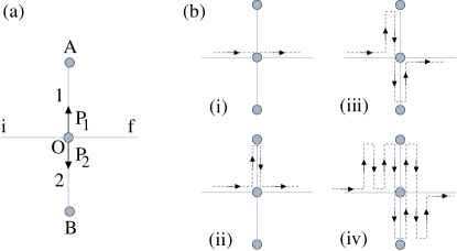
Figure 4: (Color online). The cross shaped graph, with two leads, $i$ and $f$ (left and right), two finite edges, 1 and 2 (up and down), and three vertices, $A$, $O$, $B$. (a) The $P_{s}$’s represent all the trajectories starting at vertex $O$ along an edge $s$ and finally tunneling $O$, to get to the lead $f$. (b) Four schematic examples of possible sp.

The cross-shaped graph is shown in Fig. 4. It is composed by three vertices, two edges and two leads. Observe that the vertex $O$ is the origin (end) of the lead $f$ ($i$). Let us first discuss the Green’s function for the particle leaving $x_{i}$, along the lead $i$, and getting to $x_{f}$, along the lead $f$. In the sum Eq. (13), the sp are all the trajectories starting from $i$, suffering multiple transmissions and reflections between the edges $1$ and $2$ (of lengths $\ell_{1}$ and $\ell_{2}$), and arriving at $f$. In Fig. 4 (b) we show schematic examples of possible sp: (i) direct transmission from $i$ to $f$ through the central vertex $O$, so that $W_{sp}=t_{O}^{(f,i)}$ and $L_{sp}=x_{f}+x_{i}$; (ii) transmission from $i$ to the edge $1$, a reflection at vertex $A$, and a final transmission from the central vertex to the lead $f$, then $W_{sp}=t_{O}^{(1,i)}\,r_{A}^{(1)}\,t_{O}^{(f,1)}$ and $L_{sp}=x_{f}+x_{i}+2\ell_{1}$; (iii) transmission to edge $1$, a reflection from $A$, then a transmission to edge $2$, a new reflection, this time from vertex $B$, and finally at $O$ a transmission to lead $f$, in this way $W_{sp}=t_{O}^{(1,i)}\,r_{A}^{(1)}\,t_{O}^{(2,1)}\,r_{B}^{(2)}\,t_{O}^{(f,2)}$ and $L_{sp}=x_{f}+x_{i}+2(\ell_{1}+\ell_{2})$; (iv) transmission to edge $1$, a double bouncing within edge $1$, then transmission to edge $2$, a reflection from vertex $B$, a transmission to edge $1$, a reflection from vertex $A$, another transmission to edge $2$, a reflection from vertex $B$, and finally a transmission to lead $f$ from edge $2$ (through vertex $O$), thus $W_{sp}=t_{O}^{(1,i)}\,[r_{A}^{(1)}]^{3}\,r_{O}^{(1)}\,[t_{O}^{(2,1)}]^{2}\,[r_{B}^{(2)}]^{2}\,t_{O}^{(1,2)}\,t_{O}^{(f,2)}$ and $L_{sp}=x_{f}+x_{i}+6\ell_{1}+4\ell_{2}$.

Such infinite large proliferation of paths can be factorized in a simple way. Indeed, since for any sp we have initially a propagation from $x_{i}$ to $O$ along $i$ and finally a propagation from $O$ to $x_{f}$ along $f$, we can write

$$G_{fi}(x_{f},x_{i};k)=\frac{\mu}{i\hbar^{2}k}\,T_{fi}\,\exp[ik(x_{f}+x_{i})].$$ (22)

Here $T_{fi}$ comprises all the contributions resulting from sp in the region $A$—$O$—$B$ of the graph, or

$$T_{fi}=\left\{\begin{array}[]{l}t_{O}^{(f,i)}\\ t_{O}^{(1,i)}\,P_{1}\\ t_{O}^{(2,i)}\,P_{2}\end{array}\right..$$ (23)

As before, the symbol ‘$\{$’ represents the trajectories splitting, which reads

$$T_{fi}=t_{O}^{(f,i)}\,+t_{O}^{(1,i)}\,P_{1}+t_{O}^{(2,i)}\,P_{2}.$$ (24)

The first term is just the amplitude for the direct path, i.e., a simple tunneling from $i$ to $f$ through $O$. The second (third) term represents the tunneling from lead $i$ to edge 1 (2) and all the subsequent possible trajectories that the particle can follow until reaching lead $f$, represented by $P_{1}$ and $P_{2}$, Fig. 4 (a).

The reasoning to obtain the two families of infinite trajectories, $P_{1}$ and $P_{2}$, is quite simple. Take, for instance, $P_{1}$: all such paths start at $x_{1}=0^{+}$, travel along edge 1 towards vertex $A$, suffer a reflection at $A$, and then return to vertex $O$. This part of the trajectories results in the term $r_{A}^{(1)}\,\exp[2ik\ell_{1}]$. Once reaching back vertex $O$ they can either, be reflected from it, then going into the set of paths $P_{1}$ again, or to tunnel to edge $2$, so going into the family of paths $P_{2}$, or yet to tunnel to lead $f$, thus terminating the $A$—$O$—$B$ part of the sp. The same type of analysis follows for $P_{2}$, so

$$\left\{\begin{array}[]{l}P_{1}=r_{A}^{(1)}\exp[2ik\ell_{1}]\left\{\begin{array}[]{l}r_{O}^{(1)}P_{1}\\ t_{O}^{(2,1)}P_{2}\\ t_{O}^{(f,1)}\end{array}\right.\\ P_{2}=r_{B}^{(2)}\exp[2ik\ell_{2}]\left\{\begin{array}[]{l}r_{O}^{(2)}P_{2}\\ t_{O}^{(1,2)}P_{1}\\ t_{O}^{(f,2)}\end{array}\right.\end{array}\right.,$$ (25)

leading to the algebraic equations

$$\left\{\begin{array}[]{l}P_{1}=r_{A}^{(1)}\exp[2ik\ell_{1}]\,\Big{(}r_{O}^{(1)}P_{1}+t_{O}^{(2,1)}P_{2}+t_{O}^{(f,1)}\Big{)}\\ P_{2}=r_{B}^{(2)}\exp[2ik\ell_{2}]\,\Big{(}r_{O}^{(2)}P_{2}+t_{O}^{(1,2)}P_{1}+t_{O}^{(f,2)}\Big{)},\end{array}\right.$$ (26)

whose solution reads

$$P_{1}={} \frac{1}{g}\left\{r_{A}^{(1)}t_{O}^{(f,1)}\exp[2ik\ell_{1}]+r_{A}^{(1)}r_{B}^{(2)}\Big{(}t_{O}^{(2,1)}t_{O}^{(f,2)}-r_{O}^{(2)}t_{O}^{(f,1)}\Big{)}\exp[2ik(\ell_{1}+\ell_{2})]\right\},$$

$$P_{2}= \frac{1}{g}\left\{r_{B}^{(2)}t_{O}^{(f,2)}\exp[2ik\ell_{2}]+r_{A}^{(1)}r_{B}^{(2)}\Big{(}t_{O}^{(1,2)}t_{O}^{(f,1)}-r_{O}^{(1)}t_{O}^{(f,2)}\Big{)}\exp[2ik(\ell_{1}+\ell_{2})]\right\},$$

for

$$g=\Big{(}1-r_{A}^{(1)}r_{O}^{(1)}\exp[2ik\ell_{1}]\Big{)}\Big{(}1-r_{B}^{(2)}r_{O}^{(2)}\exp[2ik\ell_{2}]\Big{)}-r_{A}^{(1)}r_{B}^{(2)}t_{O}^{(2,1)}t_{O}^{(1,2)}\exp[2ik(\ell_{1}+\ell_{2})].$$ (28)

Similarly, we can consider both the initial and end points at the edge $i$ ($0\leq x_{i},x_{f}<+\infty\in i$), for which $G_{ii}$ is given by

$$G_{ii}(x_{f},x_{i};k)=\frac{\mu}{i\hbar^{2}k}\Big{\{}\exp[ik|x_{f}-x_{i}|]+R_{ii}\,\exp[ik(x_{f}+x_{i})]\Big{\}}.$$ (29)

In this case, it is not difficult to see that

$$R_{ii}=r_{O}^{(i)}+t_{O}^{(1,i)}P_{1}+t_{O}^{(2,i)}P_{2}.$$ (30)

The expressions leading to the correct $P$’s are those in (LABEL:eq:ps-cross) where, however, we must make the obvious substitution of $t_{O}^{(f,s)}$ by $t_{O}^{(i,s)}$ ($s=1,2$).

Finally, we consider the end point $x_{f}$ in one of the edges, say edge $1$. We assume that the origin of the this edge is at vertex $O$, so $0<x_{f}<\ell_{1}$. Then, we have that

$$G_{1i}(x_{f},x_{i};k)=\frac{\mu}{i\hbar^{2}k}\,\exp[ikx_{i}]\,\Big{(}t_{O}^{(1,i)}P_{1}+t_{O}^{(2,i)}P_{2}\Big{)}.$$ (31)

Of course here we should not take into account any sp for which the particle tunnels to the edge $f$ or comes back to the edge $i$ (for a reason similar to that explained in footnote 7). Thus, we have for the $P$’s:

$$\left\{\begin{array}[]{l}P_{1}=\exp[ikx_{f}]+r_{A}^{(1)}\,\exp[2ik\ell_{1}]\,\Big{(}\exp[-ikx_{f}]+r_{O}^{(1)}\,P_{1}+t_{O}^{(2,1)}\,P_{2}\Big{)}\\ P_{2}=r_{B}^{(2)}\,\exp[2ik\ell_{2}]\,\Big{(}r_{O}^{(2)}\,P_{2}+t_{O}^{(1,2)}\,P_{1}\Big{)}.\end{array}\right.$$ (32)

By solving the above system and substituting into the expression (31), we get

$$G_{1i}(x_{f},x_{i};k)={} \frac{\mu}{i\hbar^{2}k}\,\frac{1}{g}\,\Big{\{}t_{O}^{(1,i)}+r_{B}^{(2)}\Big{(}t_{O}^{(2,i)}t_{O}^{(1,2)}-r_{O}^{(2)}t_{O}^{(1,i)}\Big{)}\exp[2ik\ell_{2}]\Big{\}}$$

$$\times\Big{\{}\exp[ik(x_{f}+x_{i})]+r_{A}^{(1)}\exp[ik(2\ell_{1}-x_{f}+x_{i})]\Big{\}},$$ (33)

with $g$ given by Eq. (28).

4.2.2 Treating a graph in terms of blocks: a tree-like case study

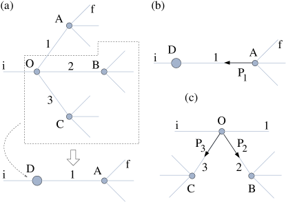
Figure 5: (Color online). A tree-like quantum graph. (a) By regarding the whole region $C$—$O$—$B$ (including the leads) as an ‘unique’ effective vertex $D$, the original graph is reduced as illustrated. (b) In the reduced graph, $P_{1}$ represents the family of trajectories which suffer multiple reflections between $D$ and $A$, and finally tunnel the vertex $A$ to the lead $f$. (c) The auxiliary graph (and the corresponding sp families) necessary to calculate $r_{D}^{(1)}$ and $t_{D}^{(i,1)}$.

Next we discuss how to shorten the calculations for a large quantum graph by decomposing it in blocks. For so, we consider the example shown in Fig. 5 (a), a relatively simple tree-like graph: a lead $i$ is attached to a vertex $O$, from which emerges three edges 1, 2 and 3, ending, respectively, at vertices $A$, $B$, and $C$. Each of these vertices, by their turn, are connected to three leads.

Here we just analyze the Green’s function for the initial position $x_{i}$ in lead $i$ and the end position $x_{f}$ in lead $f$ (this latter lead, $f$, connected to vertex $A$, see Fig. 5 (a)). Observe that in this particular situation we do not need to consider any sp that goes into another lead besides $f$ (because then, it would be impossible for the particle to come back to $f$).

The first step to simplify the problem is to treat the whole block indicated in Fig. 5 (a) as a single vertex $D$. Any information about the inner structure of such region will be contained in the vertex quantum amplitudes $t_{D}^{(1,i)}$ and $r_{D}^{(1)}$. Thus, we reduce the original graph to the simpler one depicted in Fig. 5 (b). From Fig. 5 (b), we have that the Green’s function can be written as $G_{fi}(x_{f},x_{i};k)=\mu/(i\hbar^{2}k)\,T_{fi}\,\exp[ik(x_{f}+x_{i})]$, with $T_{fi}=t_{D}^{(1,i)}\exp[ik\ell_{1}]\Big{(}r_{A}^{(1)}P_{1}+t_{A}^{(f,1)}\Big{)}$. Then, based on our previous discussions, one quickly realizes that the infinite family of trajectories $P_{1}$ is given by $P_{1}=r_{D}^{(1)}\exp[2ik\ell_{1}]\Big{(}r_{A}^{(1)}P_{1}+t_{A}^{(f,1)}\Big{)}$, or

$$P_{1}=\frac{r_{D}^{(1)}t_{A}^{(f,1)}\exp[2ik\ell_{1}]}{1-r_{D}^{(1)}r_{A}^{(1)}\,\exp[2ik\ell_{1}]}.$$ (34)

It remains to determine the coefficients $t_{D}^{(1,i)}$ and $r_{D}^{(1)}$. We can do so with the help of the auxiliary quantum graph of Fig. 5 (c). We first recall that $t_{D}^{(1,i)}$ ($r_{D}^{(1)}$) represents the sp contribution for the particle to go from lead $i$ (edge $1$) to edge $1$ through the region $B$—$O$—$C$. Inspecting Fig. 5 (c), we see that $t_{D}^{(1,i)}=t_{O}^{(1,i)}+t_{O}^{(3,i)}P_{3}+t_{O}^{(2,i)}P_{2}$ and $r_{D}^{(1)}=r_{O}^{(1)}+t_{O}^{(3,1)}P_{3}+t_{O}^{(2,1)}P_{2}$, where for the $P$’s

$$\left\{\begin{array}[]{l}P_{3}=r_{C}^{(3)}\exp[2ik\ell_{3}]\Big{(}r_{O}^{(3)}P_{3}+t_{O}^{(2,3)}P_{2}+t_{O}^{(1,3)}\Big{)}\\ P_{2}=r_{B}^{(2)}\exp[2ik\ell_{2}]\Big{(}r_{O}^{(2)}P_{2}+t_{O}^{(3,2)}P_{3}+t_{O}^{(1,2)}\Big{)}.\end{array}\right.$$ (35)

The solution of Eq. (35) is given by Eq. (LABEL:eq:ps-cross) with the appropriate labels substitutions in (LABEL:eq:ps-cross): $A\rightarrow C$, $1\rightarrow 3$ and $f\rightarrow 1$.

4.3 The Green’s function solutions by eliminating, redefining or regrouping scattering amplitudes

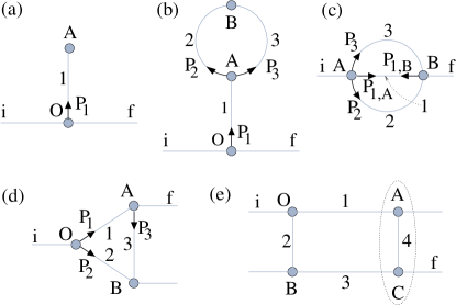
Figure 6: (Color online). Several graphs whose $G$’s can be obtained from the solutions of other topologies by eliminating, redefining or regrouping the vertices reflections and transmissions quantum amplitudes. (a) The cross shaped graph, Fig. 4, but with both the bottom edge and vertex removed. (b) The same as in (a), but with the simple vertex $A$ substituted by a circle-like structure. (c) A circle-like graph attached to two leads. (d) Triangle (e) and rectangle graphs attached to semi-infinite leads.

A great advantage in writing the Green’s function in terms of the general scattering amplitudes of each vertex is that by setting appropriate values for or regrouping these quantities, we can obtain $G$ for some graphs based on the solutions for other topologies.

Indeed, for a vertex $j$ attached to two edges ($e_{j_{1}}$ and $e_{j_{2}}$), to set $r_{j}^{(s)}=0$ and $t_{j}^{(s,r)}=1$ ($s,r=1,2$) is equivalent to remove the vertex $j$ from the graph. On the other hand, if for all $e_{j_{r}}$ we set $t_{j}^{(s,r)}=0$ for the two (one) vertices $j$ attached to the finite (semi-infinite) edge $e_{j_{s}}$, then we eliminate $e_{j_{s}}$ from the structure. For instance, consider the graph in Fig. 6 (a). We obtain its exact $G_{fi}$, $G_{ii}$ and $G_{1i}$ just by assuming $t_{O}^{(2,i)}=t_{O}^{(2,1)}=0$ for the solutions of the cross shaped graph of Fig. 4.

As for regrouping, the $G$’s for the graph in Fig. 6 (b) – if $x_{i}$ and $x_{f}$ are not in the edges $2$ and $3$ – follow from the exact Green’s functions for the graph of Fig. 6 (a) by just supposing the whole region $A$—$B$—$A$ as a single vertex, say $C$, and making the substitution $r_{A}^{(1)}\rightarrow r_{C}^{(1)}$. From the Fig. 6 (b) we see that $r_{C}^{(1)}$ is given by $r_{C}^{(1)}=r_{A}^{(1)}+t_{A}^{(2,1)}P_{2}+t_{A}^{(3,1)}P_{3}$, with the $P$’s obtained from

$$\left\{\begin{array}[]{l}P_{2}=r_{B}^{(2)}\exp[2ik\ell_{2}]\Big{(}r_{A}^{(2)}P_{2}+t_{A}^{(3,2)}P_{3}+t_{A}^{(1,2)}\Big{)}\\ \ \ \ \ \ \ +t_{B}^{(3,2)}\exp[ik(\ell_{2}+\ell_{3})]\Big{(}r_{A}^{(3)}P_{3}+t_{A}^{(2,3)}P_{2}+t_{A}^{(1,3)}\Big{)}\\ P_{3}=r_{B}^{(3)}\exp[2ik\ell_{3}]\Big{(}r_{A}^{(3)}P_{3}+t_{A}^{(2,3)}P_{2}+t_{A}^{(1,3)}\Big{)}\\ \ \ \ \ \ \ +t_{B}^{(2,3)}\exp[ik(\ell_{2}+\ell_{3})]\Big{(}r_{A}^{(2)}P_{2}+t_{A}^{(3,2)}P_{3}+t_{A}^{(1,2)}\Big{)}.\end{array}\right.$$ (36)

Consider now the more involving example in Fig. 6 (c) and $G_{11}$ for which both end points are in edge $1$, i.e., $0<x_{i},x_{f}<\ell_{1}$. We define $r_{C}^{(1)}$ ($t_{C}^{(1,1)}$) as the resulting quantum amplitude for the particle to hit the vertex $A$ from edge 1, to suffer all the multiple scattering in edges $2$ and $3$ and finally to come back to edge 1 from the vertex $A$ ($B$). We likewise define $r_{D}^{(1)}$ and $t_{D}^{(1,1)}$ for the particle initially hitting the vertex $B$. So, we have that (dropping the superscripts $(1)$ and $(1,1)$ for simplicity)

$$G_{11}(x_{f},x_{i};k)=\frac{\mu}{i\hbar^{2}k}\Big{\{}\exp[ik|x_{f}-x_{i}|]+\exp[ik(\ell_{1}-x_{i})]\Big{(}r_{D}P_{1,B}+t_{D}P_{1,A}\Big{)}+\exp[ikx_{i}]\Big{(}r_{C}P_{1,A}+t_{C}P_{1,B}\Big{)}\Big{\}},$$ (37)

where

$$\left\{\begin{array}[]{l}P_{1,A}=\exp[ikx_{f}]+\exp[ik\ell_{1}]\Big{(}r_{D}P_{1,B}+t_{D}P_{1,A}\Big{)}\\ P_{1,B}=\exp[ik(\ell_{1}-x_{f})]+\exp[ik\ell_{1}]\Big{(}r_{C}P_{1,A}+t_{C}P_{1,B}\Big{)}.\end{array}\right.$$ (38)

Solving the above system, the Green’s function (37) reads

$$G_{11}(x_{f},x_{i};k)={} \frac{\mu}{i\hbar^{2}k}\,\frac{1}{g}\,\Big{\{}g\exp[ik|x_{f}-x_{i}|]+r_{C}\exp[ik(x_{f}+x_{i})]+r_{D}\exp[ik(2\ell_{1}-x_{f}+x_{i})]$$

$$+r_{C}\,r_{D}\exp[ik(2\ell_{1}+x_{f}-x_{i})]+r_{C}\,r_{D}\exp[ik(2\ell_{1}-x_{f}+x_{i})]$$

$$+\Big{(}1-t_{C}\exp[ik\ell_{1}]\Big{)}\exp[ik(\ell_{1}+x_{f}-x_{i})]$$

$$+\Big{(}1-t_{D}\exp[ik\ell_{1}]\Big{)}\exp[-ik(\ell_{1}-x_{f}+x_{i})]\Big{\}},$$ (39)

with $g=\Big{(}1-t_{C}\exp[ik\ell_{1}]\Big{)}\Big{(}1-t_{D}\exp[ik\ell_{1}]\Big{)}-r_{C}\,r_{D}\exp[2ik\ell_{1}]$.

Above, the coefficient $r_{C}$ (see Fig. 6 (c)) is given by $r_{C}=r_{A}^{(1)}+t_{A}^{(2,1)}P_{2}+t_{A}^{(3,1)}P_{3}$, with $P_{2}$ and $P_{3}$ obeying to

$$\left\{\begin{array}[]{l}P_{2}=r_{B}^{(2)}\exp[2ik\ell_{2}]\left(r_{A}^{(2)}\,P_{2}+t_{A}^{(3,2)}\,P_{3}+t_{A}^{(1,2)}\right)\\ \ \ \ \ \ \ \,+t_{B}^{(3,2)}\exp[ik(\ell_{2}+\ell_{3})]\left(r_{A}^{(3)}\,P_{3}+t_{A}^{(2,3)}\,P_{2}+t_{A}^{(1,3)}\right)\\ P_{3}=r_{B}^{(3)}\exp[2ik\ell_{3}]\left(r_{A}^{(3)}\,P_{3}+t_{A}^{(2,3)}\,P_{2}+t_{A}^{(1,3)}\right)\\ \ \ \ \ \ \ \,+t_{B}^{(2,3)}\exp[ik(\ell_{2}+\ell_{3})]\left(r_{A}^{(2)}\,P_{2}+t_{A}^{(3,2)}\,P_{3}+t_{A}^{(1,2)}\right)\end{array}\right..$$ (40)

By its turn $t_{C}=t_{A}^{(2,1)}P_{2}+t_{A}^{(3,1)}P_{3}$, where instead of Eq. (40) this time $P_{2}$ and $P_{3}$ satisfy to

$$\left\{\begin{array}[]{l}P_{2}=r_{B}^{(2)}\exp[2ik\ell_{2}]\left(r_{A}^{(2)}\,P_{2}+t_{A}^{(3,2)}\,P_{3}\right)\\ \ \ \ \ \ \ \,+t_{B}^{(3,2)}\exp[ik(\ell_{2}+\ell_{3})]\left(r_{A}^{(3)}\,P_{3}+t_{A}^{(2,3)}\,P_{2}\right)+\exp[ik\ell_{2}]t_{B}^{(1,2)}\\ P_{3}=r_{B}^{(3)}\exp[2ik\ell_{3}]\left(r_{A}^{(3)}\,P_{3}+t_{A}^{(2,3)}\,P_{2}\right)\\ \ \ \ \ \ \ \,+t_{B}^{(2,3)}\exp[ik(\ell_{2}+\ell_{3})]\left(r_{A}^{(2)}\,P_{2}+t_{A}^{(3,2)}\,P_{3}\right)+\exp[ik\ell_{3}]t_{B}^{(1,3)}\end{array}\right..$$ (41)

The amplitudes $r_{D}$ and $t_{D}$ are obtained from the expression for $r_{C}$ and $t_{C}$ by just exchanging the indices $A\leftrightarrow B$.

Finally, if for both graphs of Fig. 6 (d) and (e), the $G$ initial and final points are, respectively, in the edges $i$ and $f$, the Green’s function is simply

$$G_{fi}(x_{f},x_{i};k)=\frac{\mu}{i\hbar^{2}k}T_{fi}\exp[ik(x_{f}+x_{i})].$$ (42)

For the case of Fig. 6 (d), $T_{fi}=t_{O}^{(1,i)}\,P_{1}+t_{O}^{(2,i)}\,P_{2}$, with $P_{1}$ and $P_{2}$ obtained from the following

$$\left\{\begin{array}[]{l}P_{1}=r_{A}^{(1)}\exp[2ik\ell_{1}]\Big{(}r_{O}^{(1)}P_{1}+t_{O}^{(2,1)}P_{2}\Big{)}+\exp[ik\ell_{1}]\Big{(}t_{A}^{(3,1)}P_{3}+t_{A}^{(f,1)}\Big{)}\\ P_{2}=r_{B}^{(2)}\exp[2ik\ell_{2}]\Big{(}r_{O}^{(2)}P_{2}+t_{O}^{(1,2)}P_{1}\Big{)}\\ \ \ \ \ \ \ +t_{B}^{(3,2)}\exp[ik(\ell_{2}+\ell_{3})]\Big{(}r_{A}^{(3)}P_{3}+t_{A}^{(f,3)}\Big{)}\\ \ \ \ \ \ \ +t_{B}^{(3,2)}t_{A}^{(1,3)}\exp[ik(\ell_{1}+\ell_{2}+\ell_{3})]\Big{(}r_{O}^{(1)}P_{1}+t_{O}^{(2,1)}P_{2}\Big{)}\\ P_{3}=r_{B}^{(3)}\exp[2ik\ell_{3}]\Big{(}r_{A}^{(3)}P_{3}+t_{A}^{(f,3)}\Big{)}\\ \ \ \ \ \ \ +t_{B}^{(2,3)}\exp[ik(\ell_{2}+\ell_{3})]\Big{(}r_{O}^{(2)}P_{2}+t_{O}^{(1,2)}P_{1}\Big{)}\\ \ \ \ \ \ \ +r_{B}^{(3)}t_{A}^{(1,3)}\exp[ik(\ell_{1}+2\ell_{3})]\Big{(}r_{O}^{(1)}P_{1}+t_{O}^{(2,1)}P_{2}\Big{)},\end{array}\right.$$ (43)

with $P_{3}$ an auxiliary family of infinite trajectories, introduced just to help in the recursive definitions of $P_{1}$ and $P_{2}$ (see Fig. 6 (d)). The solution of the above system put into the expression for $T_{fi}$ yields the final exact Green’s function.

For $G_{fi}$ for the graph of Fig. 6 (e) we can use the above same set of equations if we treat the region comprising vertices $A$ and $C$ of Fig. 6 (e) as a single effective vertex, corresponding to $A$ in Fig. 6 (d). Thus, by using the previous analysis, we find that we need only to make the following substitutions in the Green’s function expression for the graph of Fig. 6 (d) so to get that for Fig. 6 (e):

$$r_{A}^{(1)}\rightarrow{} \,r_{A}^{(1)}+t_{A}^{(4,1)}\,r_{C}^{(4)}\,t_{A}^{(1,4)}\exp[2ik\ell_{4}]/g,$$

$$t_{A}^{(f,1)}\rightarrow{} t_{A}^{(4,1)}\,t_{C}^{(f,4)}\exp[ik\ell_{4}]/g,$$

$$t_{A}^{(3,1)}\rightarrow{} t_{A}^{(4,1)}\,t_{C}^{(3,4)}\exp[ik\ell_{4}]/g,$$

$$r_{A}^{(3)}\rightarrow{} r_{C}^{(3)}+t_{C}^{(4,3)}\,r_{A}^{(4)}\,t_{C}^{(3,4)}\exp[2ik\ell_{4}]/g,$$

$$t_{A}^{(f,3)}\rightarrow{} t_{C}^{(f,3)}+t_{C}^{(4,3)}\,r_{A}^{(4)}t_{C}^{(f,4)}\exp[2ik\ell_{4}]/g,$$

$$t_{A}^{(1,3)}\rightarrow{} t_{C}^{(4,3)}\,t_{A}^{(1,4)}\exp[ik\ell_{4}]/g,$$

where $g=1-r_{A}^{(4)}\,r_{C}^{(4)}\exp[2ik\ell_{4}]$.

5 Eigenstates and scattering states in quantum graphs

From the previous Sec. we have seen that different techniques enable one to obtain $G$ in a relatively straightforward way. Moreover, we also have mentioned that the calculation of the wave function in certain contexts might be lengthy. Therefore, a natural question is how easily one can extract from $G$ the system eigenvalues, eigenstates and scattering states, thus allowing to bypass the more traditional approach of directly solving the Schrödinger equation. Next we give some examples along this line. For definiteness, we concentrate on the graph of Fig. 6 (a).

5.1 Eigenstates

The explicit expression for the Green’s function with $x_{i}$ in lead $i$ and $x_{f}$ in lead $f$ is (Fig. 6 (a))

$$G_{fi}(x_{f},x_{i};k)={} \frac{\mu}{i\hbar^{2}k}\,T_{fi}\,\exp[ik(x_{f}+x_{i})],$$

$$T_{fi}={} t_{O}^{(f,i)}+\frac{t_{O}^{(1,i)}\,r_{A}^{(1)}\,t_{O}^{(f,1)}\exp[2ik\ell_{1}]}{1-r_{O}^{(1)}\,r_{A}^{(1)}\exp[2ik\ell_{1}]}.$$ (44)

For both $x_{i}$ and $x_{f}$ ($0<x_{i},x_{f}<\ell_{1}$, $x_{f}>x_{i}$) in the edge $1$, we get

$$G_{11}(x_{f},x_{i};k)={} \frac{\mu}{i\hbar^{2}k}\frac{1}{\Big{(}1-r_{O}^{(1)}\,r_{A}^{(1)}\exp[2ik\ell_{1}]\Big{)}}$$

$$\times\Big{(}\exp[-ikx_{i}]+r_{O}^{(1)}\exp[ikx_{i}]\Big{)}\,\Big{(}\exp[ikx_{f}]+r_{A}^{(1)}\exp[2ik\ell_{1}]\exp[-ikx_{f}]\Big{)}.$$ (45)

For open graphs, like that in Fig. 6 (a), depending on the characteristics of the vertices, the system may support bound states. In these cases, the eigenstates are calculated from the residues of $G(x_{f},x_{i};k)$ at the poles $k=k_{n}$ [135], which give the problem eigenenergies through $E_{n}=\hbar^{2}k_{n}^{2}/(2\mu)$.

By inspecting the above Green’s functions, we see that they can diverge (consequently presenting poles [30]) only if $g(k=k_{n})=0$, with

$$g(k)=1-r_{O}^{(1)}(k)\,r_{A}^{(1)}(k)\exp[2ik\ell_{1}].$$ (46)

As a concrete example, consider the vertex $O$ being a generalized $\delta$ interaction (here attached to $N=3$ edges, Fig. 6 (a)) of strength $\gamma$ [30]. Then, for simplicity setting $\hbar=\mu=1$, the reflection coefficients for the vertex $O$ are given by (see Appendix C)

$$r_{O}^{(1)}(k)=r_{O}^{(i)}(k)=r_{O}^{(f)}(k)=r_{O}(k)=\frac{2\gamma-(N-2)ik}{Nik-2\gamma}=\frac{2\gamma-ik}{3ik-2\gamma},$$ (47)

and the transmission coefficients by

$$t_{O}^{(1,i)}(k)=t_{O}^{(f,1)}(k)=t_{O}^{(f,i)}(k)=t_{O}(k)=\frac{2ik}{Nik-2\gamma}=\frac{2ik}{3ik-2\gamma}.$$ (48)

For the vertex $A$, as discussed in the Appendix C, we take the boundary condition $-\psi^{\prime}(A)=\lambda\psi(A)$, which is equivalent to the following reflection coefficient

$$r_{A}(k)=\frac{ik+\lambda}{ik-\lambda}.$$ (49)

It is a well-known fact that any pole of the scattering amplitudes in the upper half of complex $k$-plane along the imaginary axis represents a bound energy [194]. For example, for the usual (1D) Dirac $\delta$-function with intensity $\gamma<0$ (attractive $\delta$), the transmission coefficient is $t_{\delta}=ik/(ik-\gamma)$. In this case, the unique negative energy of the system reads $E_{1}=k_{1}^{2}/2=-\gamma^{2}/2$, where $k_{1}=i|\gamma|$ is the only pole of $t_{\delta}(k)$ [195, 196].

So, for our graph the eigenvalues are obtained from the following transcendental equation (with Re$[k_{n}]=0$ and Im$[k_{n}]>0$)

$$g(k_{n})=1-\left(\frac{2\gamma-ik_{n}}{3ik_{n}-2\gamma}\right)\left(\frac{ik_{n}+\lambda}{ik_{n}-\lambda}\right)\exp[i2k_{n}\ell_{1}]=0.$$ (50)

Further, using the formula ($g^{\prime}(k_{n})\equiv\left.dg(k)/dk\right|_{k=k_{n}}$)

$$\lim_{E\rightarrow E_{n}}\frac{(E-E_{n})}{g(k)}=\frac{1}{2}\lim_{k\rightarrow k_{n}}\frac{(k^{2}-k_{n}^{2})}{g(k)}=\frac{k_{n}}{g^{\prime}(k_{n})},$$ (51)

the residues of Eq. (44) are obtained from

$$\psi_{n}^{(f)}(x_{f})\,{\psi_{n}^{(i)}}^{*}(x_{i})={} \frac{1}{2}\lim_{k\rightarrow k_{n}}(k^{2}-k_{n}^{2})\,G_{fi}(x_{f},x_{i};k)$$

$$={} \Big{\{}{\mathcal{N}}_{G}(k_{n})\,t_{O}(k_{n})\,\exp[ik_{n}x_{f}]\Big{\}}\,\Big{\{}{\mathcal{N}}_{G}(k_{n})\,t_{O}(k_{n})\,\exp[ik_{n}x_{i}]\Big{\}},$$ (52)

and of Eq. (45) from

$$\psi_{n}^{(1)}(x_{f})\,{\psi_{n}^{(1)}}^{*}(x_{i})={} \frac{1}{2}\lim_{k\rightarrow k_{n}}(k^{2}-k_{n}^{2})\,G_{11}(x_{f},x_{i};k)$$

$$={} \Big{\{}{\mathcal{N}}_{G}(k_{n})\,\Big{(}\exp[-ik_{n}x_{f}]+r_{O}^{(1)}(k_{n})\exp[ik_{n}x_{f}]\Big{)}\Big{\}}$$

$$\times\Big{\{}{\mathcal{N}}_{G}(k_{n})\,\Big{(}\exp[-ik_{n}x_{i}]+r_{O}^{(1)}(k_{n})\exp[ik_{n}x_{i}]\Big{)}\Big{\}}.$$ (53)

Observe that in the above Eqs., because after the substitution $k_{n}=i\kappa_{n}$ all the terms become real-valued functions, the complex conjugation, in this particular case, makes no practical difference. Finally

$${\mathcal{N}}_{G}(k_{n})=\frac{1}{\sqrt{ig^{\prime}(k_{n})\,r_{O}^{(1)}(k_{n})}}.$$ (54)

Note that for the poles $k_{n}=i\kappa_{n}$, with $\kappa_{n}>0$, the wave functions in both leads have the general form $\psi_{n}(x)={\mathcal{N}}\exp[-\kappa_{n}x]$ (recall that $x\geq 0$). Hence, they decay away from the origin (vertex $O$) exponentially, as it should be. The ${\mathcal{N}}$’s also lead to the correct normalization for the eigenstates. Important to mention that the same results follow from the direct solution of the Schrödinger equation with the appropriate boundary conditions (which is done in the Appendix C).

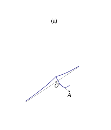
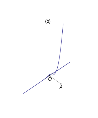
Figure 7: (Color online). The bound eigenstates probability distribution along the quantum graph of Fig. 6 (a), here with $\ell_{1}=1$. The vertex $O$ is a $\delta$ interaction of strength $\gamma=-3/2$. The boundary condition at the vertex $A$ is given by $-\psi^{\prime}(A)=\lambda\psi(A)$, with $\lambda=-2$. (a) $|\psi_{1}(x)|^{2}$ for which $\kappa_{1}=0.463618$ and (b) $|\psi_{2}(x)|^{2}$ for which $\kappa_{2}=2.022448$.

As a numerical example, consider $\gamma=-3/2$, $\lambda=-2$, and $\ell_{1}=1$. Then, the system has two bound eigenstates, $n=1,2$. In Fig. 7 we show the corresponding $|\psi_{n}(x)|^{2}$. The first (second) eigenstate, with $\kappa_{1}=0.463618$ ($\kappa_{2}=2.022448$), is mainly due to the attractive $\delta$ potential (to the boundary condition at the vertex $A$). This can verified in Fig. 7: $|\psi_{1}|^{2}$ ($|\psi_{2}|^{2}$) is much more concentrated around the vertex $O$ ($A$).

5.2 Scattering

Consider again the Green function $G_{fi}$, Eq. (44), for the open graph of Fig. 6 (a). As already discussed, the quantity $|T_{fi}|^{2}$ (in $G_{fi}$) can be interpreted as the total probability for a particle of wave number $k$ incident from the lead $i$ to be transmitted to the lead $f$. Similarly, supposing $x_{i}$ and $x_{f}$ in lead $i$, we have

$$G_{ii}(x_{f},x_{i};k)={} \frac{\mu}{i\hbar^{2}k}\Big{\{}\exp[ik|x_{f}-x_{i}|]+R_{i}\exp[ik(x_{f}+x_{i})]\Big{\}},$$

$$R_{i}={} r_{O}^{(i)}+\frac{t_{O}^{(1,i)}\,r_{A}^{(1)}\,t_{O}^{(i,1)}\exp[2ik\ell_{1}]}{1-r_{O}^{(1)}\,r_{A}^{(1)}\exp[2ik\ell_{1}]}.$$ (55)

Then, $|R_{i}|^{2}$ represents the total probability for a particle of wave number $k$ incident from the lead $i$ to be reflected to the lead $i$. By choosing different quantum amplitudes for the vertices, we naturally get different scattering patterns from $R_{i}$ and $T_{fi}$.

To illustrate possible different scattering behavior for this graph, we assume the Neumann-Kirchhoff boundary conditions (Appendix C) at the vertex $A$, so we set $\lambda=0$ in Eq. (49). For $O$, we consider three values for the parameter $\gamma$: (a) $\gamma=0$ (so, also Neumann-Kirchhoff); and the generalized $\delta$ of strengths (b) $\gamma=1$ and (c) $\gamma=-3/2$. The resulting $|R_{i}|^{2}$ and $|T_{fi}|^{2}$ as function of $k$ are shown in Fig. 8, where distinctions in the scattering probabilities are clearly observed. In all cases $\ell_{1}=1$.

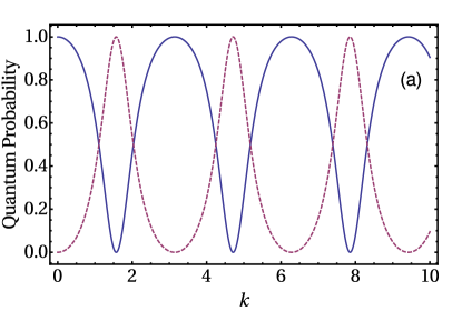
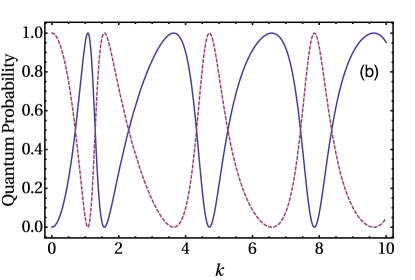
Figure 8: (Color online). The transmission $|T_{fi}|^{2}$ (solid line) and reflection $|R_{i}|^{2}$ (dashed) probabilities as function of $k$ for the quantum graph of Fig. 6 (a). In all cases $\ell_{1}=1$ and $\lambda=0$ (Neumann-Kirchhoff boundary conditions at $A$). The values of $\gamma$ at $O$ are: (a) 0, (b) 1, and (c) -3/2.

6 Representative quantum graphs

So far we have discussed the general ideas of how to use the energy domain Green’s function method to study quantum graphs through the explicit calculation of arbitrary cases. But in the literature one can find certain topologies which are particularly convenient and flexible to model many distinct quantum phenomena. For instance, the examples already addressed in Sec. 4, Fig. 6, are indeed proper structures to construct logic gates for quantum information processing [66, 68]. In special, the graph in Fig. 6 (b) can act as a phase shifter, whereas that in Fig. 6 (e) could functioning as a basis-changing gate.

Other very important examples include:

• The widely analyzed (with the most distinct purposes [71, 197, 198, 199, 200], like to investigate scattering features of 3D graphs [201]) hypercube;

• The binary tree [202, 203, 204], e.g., useful to highlight differences between classical and quantum walks [205] as well as to test the speed up gain – which is actually exponential – in searching algorithms based on quantum dynamics [206]. We should observe that the graph of Fig. 5 (a) is in fact an extension of a binary tree, being a fragment of a large-scale ternary tree network [207];

• Triangular Sierpiński-like structures [208], a nice illustration of graphs which in the limit of infinite vertices would be fractal. It has been considered in connection with molecular assembling [209] and with the mathematics of logical games like the Hanoi tower [210, 211].

Given the relevance of the above mentioned three graph systems, in the present section we show in details how to calculate the exact Green’s function for each one of these problems.

6.1 Cube

Figure 9: (Color online). A cube quantum graph. (a) The letters represent the vertices indices and the integers the edges indices. (b) A cube graph planar representation. (c)-(e) Regrouping procedures (see the main text). (f) Auxiliary graph to determine the total $R$’s and $T$’s. (g) The inner structure of vertex $I$. The $P_{l}$’s indicate the sp families.

The Green’s function for closed quantum graphs can be obtained by the regrouping technique discussed in the previous sections. Thus, we will use this procedure to get the Green’s function for the cube quantum graph of Fig. 9 (a) (where all edges have length $\ell$). In Fig. 9 (b) we show a planar representation of the cube graph. For concreteness, let us suppose both the initial and final positions in the edge $1$ (see Fig. 9 (a)). The first step to simplify the calculations is to view the two regions marked by dashed lines in Fig. 9 (c) as two vertices $I$ and $J$, Fig. 9 (d). The second is a further regrouping, in which we represent $I$ and $J$ as a single vertex $K$, Fig. 9 (e). Therefore, we end up reducing the original cube to a simple circular graph.

Now, consider Fig. 9 (e), with $x_{f}>x_{i}$ ($x\in(0,\ell)$ increases anti-clockwise from vertex $K$). We then define for $K$ the total reflection and transmission amplitudes $R^{(\pm)}$ and $T^{(\pm)}$ (where the superscript $+$ ($-$) indicates that the scattering process takes place at $\ell$ ($0$)). In this way, all the information about the internal structure of the cube graph are contained in these $K$ vertex coefficients. Thus, for the circular graph of Fig. 9 (e), the Green’s function can be written as

$$G_{11}(x_{f},x_{i};k)={} \frac{\mu}{i\hbar^{2}k}\left\{\exp[ik(x_{f}-x_{i})]+\exp[ikx_{i}]\,\left(R^{(-)}\,P_{1K}+T^{(-)}\,P_{2K}\right)\right.$$

$$+\left.\exp[ik(\ell-x_{i})]\,\left(R^{(+)}\,P_{2K}+T^{(+)}\,P_{1K}\right)\right\},$$ (56)

with $P_{1K}$ and $P_{2K}$ given by

$$\left\{\begin{array}[]{l}P_{1K}=\exp[ikx_{f}]+\exp[ik\ell]\left(R^{(+)}\,P_{2K}+T^{(+)}\,P_{1K}\right),\\ P_{2K}=\exp[ik(\ell-x_{f})]+\exp[ik\ell]\left(R^{(-)}\,P_{1K}+T^{(-)}\,P_{2K}\right).\end{array}\right.$$ (57)

Solving the above system, the Green’s function (56) reads

$$G_{11}(x_{f},x_{i};k)={} \frac{\mu}{i\hbar^{2}k}\frac{1}{g}\Big{\{}\Big{(}1-T^{(-)}\exp[ik\ell]\Big{)}\exp[ik(x_{f}-x_{i})]$$

$$+R^{(-)}\exp[ik(x_{f}+x_{i})]+R^{(+)}\exp[ik(2\ell-x_{f}-x_{i})]$$

$$+\Big{(}T^{(-)}+\Big{(}R^{(+)}\,R^{(-)}-T^{(+)}\,T^{(-)}\Big{)}\exp[ik\ell]\Big{)}\exp[ik(\ell-x_{f}+x_{i})]\Big{\}},$$ (58)

with

$$g=(1-T^{(+)}\exp[ik\ell])\,(1-T^{(-)}\exp[ik\ell])-R^{(+)}\,R^{(-)}\exp[2ik\ell].$$ (59)

Next, we must determine the coefficients $R$’s and $T$’s. We do so with help of the auxiliary quantum graph in Fig. 9 (f). We recall that $T^{(\pm)}$ ($R^{(\pm)}$) represents the paths contribution for the particle going from edge 1 to edge 1 by means of a transmission through (reflection from) the vertex $K$. Inspecting Fig. 9 (e) and (f), we see that the transmission from $I$ ($J$) to $J$ ($I$) yields $T^{(-)}$ ($T^{(+)}$). Similarly, the reflection from $I$ ($J$) leads to $R^{(-)}$ ($R^{(+)}$). We start with $T^{(-)}$, then

$$T^{(-)}={} t_{I}^{(3,1)}\,\exp[ik\ell]\,\Big{(}r_{J}^{(3)}\,P_{3}+t_{J}^{(9,3)}\,P_{9}+t_{J}^{(11,3)}\,P_{11}+t_{J}^{(1,3)}\Big{)}$$

$$+t_{I}^{(9,1)}\,\exp[ik\ell]\,\Big{(}r_{J}^{(9)}\,P_{9}+t_{J}^{(3,9)}\,P_{3}+t_{J}^{(11,9)}\,P_{11}+t_{J}^{(1,9)}\Big{)}$$

$$+t_{I}^{(11,1)}\,\exp[ik\ell]\,\Big{(}r_{J}^{(11)}\,P_{11}+t_{J}^{(3,11)}\,P_{3}+t_{J}^{(9,11)}\,P_{9}+t_{J}^{(1,11)}\Big{)},$$ (60)

where the $P$’s are

$$\left\{\begin{array}[]{l}P_{3}=r_{I}^{(3)}\,\exp[2ik\ell]\,\left(r_{J}^{(3)}\,P_{3}+t_{J}^{(9,3)}\,P_{9}+t_{J}^{(11,3)}\,P_{11}+t_{J}^{(1,3)}\right)\\ \ \ \ \ \,\,+\,\,t_{I}^{(9,3)}\,\exp[2ik\ell]\,\left(r_{J}^{(9)}\,P_{9}+t_{J}^{(3,9)}\,P_{3}+\,\,t_{J}^{(11,9)}\,P_{11}+t_{J}^{(1,9)}\right)\\ \ \ \ \ \,\,+\,\,t_{I}^{(11,3)}\,\exp[2ik\ell]\,\left(r_{J}^{(11)}\,P_{11}+t_{J}^{(3,11)}\,P_{3}+\,\,t_{J}^{(9,11)}\,P_{9}+t_{J}^{(1,11)}\right)\\ P_{9}=r_{I}^{(9)}\,\exp[2ik\ell]\,\left(r_{J}^{(9)}\,P_{9}+t_{J}^{(3,9)}\,P_{3}+t_{J}^{(11,9)}\,P_{11}+t_{J}^{(1,9)}\right)\\ \ \ \ \ \,\,+\,\,t_{I}^{(3,9)}\,\exp[2ik\ell]\,\left(r_{J}^{(3)}\,P_{3}+t_{J}^{(9,3)}\,P_{9}+t_{J}^{(11,3)}\,P_{11}+t_{J}^{(1,3)}\right)\\ \ \ \ \ \,\,+\,\,t_{I}^{(11,9)}\,\exp[2ik\ell]\,\left(r_{J}^{(11)}\,P_{11}+t_{J}^{(3,11)}\,P_{3}+t_{J}^{(9,11)}\,P_{9}+t_{J}^{(1,11)}\right)\\ P_{11}=r_{I}^{(11)}\,\exp[2ik\ell]\,\left(r_{J}^{(11)}\,P_{11}+t_{J}^{(3,11)}\,P_{3}+t_{J}^{(9,11)}\,P_{9}+t_{J}^{(1,11)}\right)\\ \ \ \ \ \,\,+\,\,t_{I}^{(3,11)}\,\exp[2ik\ell]\,\left(r_{J}^{(3)}\,P_{3}+t_{J}^{(9,3)}\,P_{9}+t_{J}^{(11,3)}\,P_{11}+t_{J}^{(1,3)}\right)\\ \ \ \ \ \,\,+\,\,t_{I}^{(9,11)}\,\exp[2ik\ell]\,\left(r_{J}^{(9)}\,P_{9}+t_{J}^{(3,9)}\,P_{3}+t_{J}^{(11,9)}\,P_{11}+t_{J}^{(1,9)}\right).\end{array}\right.$$ (61)

For $R^{(+)}$ we have

$$R^{(+)}=r_{J}^{(1)}+t_{J}^{(3,1)}\,P_{3}+t_{J}^{(9,1)}\,P_{9}+t_{J}^{(11,1)}\,P_{11},$$ (62)

where the $P$’s are those in Eq. (61). We obtain $T^{(+)}$ and $R^{(-)}$ from $T^{(-)}$ and $R^{(+)}$ by the simple substitution $I\leftrightarrow J$.

Finally, we shall obtain $r_{I\,(J)}$ and $t_{I\,(J)}$ in terms of the original vertices coefficients. As one might expect, because the cube symmetry the quantum amplitudes for $I$ and $J$ can be derived from each other by a direct indices relabeling . So, we just discuss in details the vertex $I$. Moreover, such type of procedure is also possible for the distinct $r_{I}^{(s)}$’s and $t_{I}^{(s,r)}$’s in Eq. (61): we can calculate, say, $r_{I}^{(1)}$, $t_{I}^{(1,3)}$, $t_{I}^{(1,11)}$, and then to infer the expressions for the others $r_{I}$’s and $t_{I}$’s by proper exchanges of vertices and edges labels.

From Fig. 9 (g), depicting the inner structure of $I$, we can write

$$r_{I}^{(1)}={} r_{A}^{(1)}+t_{A}^{(4,1)}P_{4}+t_{A}^{(5,1)}P_{5},$$

$$t_{I}^{(1,11)}={} t_{H}^{(8,11)}P_{8}+t_{H}^{(12,11)}P_{12},$$

$$t_{I}^{(1,3)}={} t_{D}^{(4,3)}\,\exp[ik\ell]\,\left(r_{A}^{(4)}\,P_{4}+t_{A}^{(5,4)}\,P_{5}+t_{A}^{(1,4)}\right)+t_{D}^{(8,3)}\,\exp[ik\ell]\,\left(r_{H}^{(8)}\,P_{8}+t_{H}^{(12,8)}\,P_{12}\right),$$ (63)

where

$$\left\{\begin{array}[]{l}P_{4}=r_{D}^{(4)}\,\exp[2ik\ell]\,\left(r_{A}^{(4)}\,P_{4}+t_{A}^{(5,4)}\,P_{5}+t_{A}^{(1,4)}\right)\\ \ \ \ \ \,\,+t_{D}^{(8,4)}\,\exp[2ik\ell]\,\left(r_{H}^{(8)}\,P_{8}+t_{H}^{(12,8)}\,P_{12}\right)\\ P_{5}=r_{E}^{(5)}\,\exp[2ik\ell]\,\left(r_{A}^{(5)}\,P_{5}+t_{A}^{(4,5)}\,P_{4}+t_{A}^{(1,5)}\right)\\ \ \ \ \ \,\,+t_{E}^{(12,5)}\,\exp[2ik\ell]\,\left(r_{H}^{(12)}\,P_{12}+t_{H}^{(8,12)}\,P_{8}\right)\\ P_{8}=t_{D}^{(4,8)}\,\exp[2ik\ell]\,\left(r_{A}^{(4)}\,P_{4}+t_{A}^{(5,4)}\,P_{5}+t_{A}^{(1,4)}\right)\\ \ \ \ \ \,\,+r_{D}^{(8)}\,\exp[2ik\ell]\,\left(r_{H}^{(8)}\,P_{8}+t_{H}^{(12,8)}\,P_{12}\right)\\ P_{12}=t_{E}^{(5,12)}\,\exp[2ik\ell]\,\left(r_{A}^{(5)}\,P_{5}+t_{A}^{(4,5)}\,P_{4}+t_{A}^{(1,5)}\right)\\ \ \ \ \ \,\,+r_{E}^{(12)}\,\exp[2ik\ell]\,\left(r_{H}^{(12)}\,P_{12}+t_{H}^{(8,12)}\,P_{8}\right).\\ \end{array}\right.$$ (64)

For $t_{I}^{(1,9)}$ we take the final expression for $t_{I}^{(1,3)}$ and perform the interchanges $D\leftrightarrow E$, $4\leftrightarrow 5$ and $8\leftrightarrow 12$. Note this is exactly the effect of a specular reflection across the diagonal $A$—$H$ of Fig. 9 (g). Actually, we can obtain all other scattering amplitudes by using this artifact of specular reflections of indices about a proper symmetry axis of the square in Fig. 9 (g). For instance, for $t_{I}^{(3,11)}$, $r_{I}^{(9)}$ and $t_{I}^{(11,1)}$, the indices exchanges applied, respectively, to $t_{I}^{(1,9)}$, $r_{I}^{(1)}$ and $t_{I}^{(1,11)}$, would be those resulting from reflections by an axis perpendicular to edges 4 and 12 ($A\leftrightarrow D$, $E\leftrightarrow H$ and $5\leftrightarrow 8$), perpendicular to edges 5 and 8 ($A\leftrightarrow E$, $D\leftrightarrow H$ and $4\leftrightarrow 12$), and in the diagonal $E$—$D$ ($A\leftrightarrow H$, $4\leftrightarrow 8$ and $5\leftrightarrow 12$).

6.1.1 Closed cube eigenenergies

Now, let us examine the closed cube graph eigenstates supposing all the vertices having the same properties. Hence, for the cube eight vertices we assume the previously discussed generalized $\delta$ interaction. Since the coordination number for this topology is $N=3$, for any vertex we set (see Eqs. (47) and (48)) $r=(2\gamma-ik)/(3ik-2\gamma)$ and $t=2ik/(3ik-2\gamma)$. The eigenenergies come from the poles of Green’s function, i.e., the roots of Eq. (59): $g=(1-T(k)\exp[ik\ell])^{2}-{R(k)}^{2}\exp[2ik\ell]=0$ (observe that in this very symmetric case, $T^{(+)}=T^{(-)}=T$ and $R^{(+)}=R^{(-)}=R$, with $R$ and $T$ obtained from the calculations described in the previous Sec.). In the Table 1 we show the resulting first ten eigenvalues for $\gamma=0$ and $\gamma=1$ (with $\mu=\hbar=1$).

	$\gamma$
State	0	1
1	1.230959	1.094322
2	1.919633	1.642395
3	3.141593	2.190764
4	4.372552	3.141593
5	5.052226	3.516328
6	6.283185	5.177393
7	7.514145	6.283185
8	8.193819	7.602957
9	9.424778	8.273085
10	10.65574	9.424778

Table 1: The first ten numerically calculated $k_{n}$ values (from $g=0$, see Eq. (59)) for the cube quantum graph. All the vertices are assumed generalized $\delta$ interactions of strength $\gamma=0$ (so, Neumann-Kirchhoff) and $\gamma=1$.

In order to check the eigenvalues found through the Green’s function approach, one can directly solve the Schrödinger equation. Along the edge $s\,(=1,\ldots,12)$, the component $\psi_{s}(x_{s})$ of the total wave function $\Psi$ is the solution of (where for simplicity we drop the subscript notation for $x$)

$$-\frac{d^{2}}{dx^{2}}\psi_{s}(x)=k^{2}\psi_{s}(x),$$ (65)

with $k=\sqrt{2\mu E}/\hbar$ and the origin for the edges taken in the vertices $A$, $C$, $F$ and $H$. Thus, the $\psi$’s have the form

$$\psi_{s}(x)={\mathcal{A}}_{s}\exp[ikx]+{\mathcal{B}}_{s}\exp[-ikx].$$ (66)

The coefficients ${\mathcal{A}}_{s}$ and ${\mathcal{B}}_{s}$ are determined by the boundary conditions, corresponding to a delta potential on the vertices (see the discussion in the Appendix C.1). Therefore

$$\psi_{1}(0)=\psi_{4}(0)=\psi_{5}(0)={} \psi(A) \psi_{1}^{\prime}(0)+\psi_{4}^{\prime}(0)+\psi_{5}^{\prime}(0)={} 2\gamma\,\psi(A)$$

$$\psi_{2}(0)=\psi_{3}(0)=\psi_{7}(0)={} \psi(C), \psi_{2}^{\prime}(0)+\psi_{3}^{\prime}(0)+\psi_{7}^{\prime}(0)={} 2\gamma\,\psi(C),$$

$$\psi_{6}(0)=\psi_{9}(0)=\psi_{10}(0)={} \psi(F), \psi_{6}^{\prime}(0)+\psi_{9}^{\prime}(0)+\psi_{10}^{\prime}(0)={} 2\gamma\,\psi(F),$$

$$\psi_{8}(0)=\psi_{11}(0)=\psi_{12}(0)={} \psi(H), \psi_{8}^{\prime}(0)+\psi_{11}^{\prime}(0)+\psi_{12}^{\prime}(0)={} 2\gamma\,\psi(H),$$

$$\psi_{1}(0)=\psi_{2}(0)=\psi_{6}(0)={} \psi(B), \psi_{1}^{\prime}(0)+\psi_{2}^{\prime}(0)+\psi_{6}^{\prime}(0)={} -2\gamma\,\psi(B),$$

$$\psi_{3}(0)=\psi_{4}(0)=\psi_{8}(0)={} \psi(D), \psi_{3}^{\prime}(0)+\psi_{4}^{\prime}(0)+\psi_{8}^{\prime}(0)={} -2\gamma\,\psi(D),$$

$$\psi_{5}(0)=\psi_{9}(0)=\psi_{12}(0)={} \psi(E), \psi_{5}^{\prime}(0)+\psi_{9}^{\prime}(0)+\psi_{12}^{\prime}(0)={} -2\gamma\,\psi(E),$$

$$\psi_{7}(0)=\psi_{10}(0)=\psi_{11}(0)={} \psi(G), \psi_{7}^{\prime}(0)+\psi_{10}^{\prime}(0)+\psi_{11}^{\prime}(0)={} -2\gamma\,\psi(G).$$ (67)

From the above system of equations – plus the normalization condition $\sum_{s=1}^{s=12}\int_{0}^{\ell}dx\,|\psi_{s}(x)|^{2}=1$ – one gets the eigenfunctions and eigenvalues. By solving Eq. (67) – e.g, numerically – one finds that the eigenvalues from the Green’s functions are exactly those from the Schrödinger equation, as it should be.

6.1.2 Scattering by attaching leads to the quantum cube graph

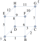
Figure 10: (Color online). The original quantum closed cube graph is attached to two leads (at the vertices $A$ and $G$), thus becoming an open graph structure.

One also can study transmission through (as well as reflection from) the original closed cube by attaching leads to it. In Fig. 10 we display a possible configuration for the system, where leads are added to the vertices $A$ and $G$ of our previous very symmetric graph. For the now modified vertices $A$ and $G$, we also assume a $\delta$ interaction of strength $\gamma$, only recalling that in this case these two vertices have a coordination number $N=4$ (instead of $N=3$). Just as an illustration, for $x_{i}$ in lead $i$ and $x_{f}$ in lead $f$ (see Fig. 10), the Green’s function reads

$$G_{fi}(x_{f},x_{i};k)=\frac{\mu}{i\hbar^{2}k}\,T_{fi}\,\exp[ik(x_{f}+x_{i})].$$ (68)

Calculating $T_{fi}$ (and also $R_{i}$) using the discussed techniques, we show in Fig. 11 the transmission and reflection probabilities as function of $k$ for $\gamma=0$ and $\gamma=1$. Since for the former the individual edges transmission and reflections coefficients are not function of $k$, we do not see $|T_{fi}|^{2}$ tending to 1 for $k$ increasing (as slowly seen for $\gamma=1$).

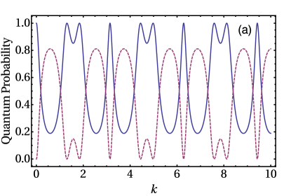
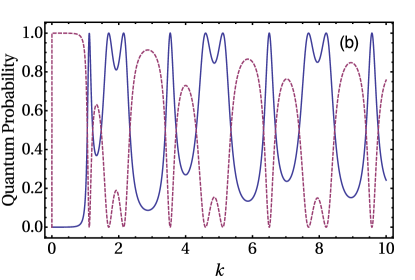
Figure 11: (Color online). The transmission $|T_{fi}|^{2}$ (solid line) and reflection $|R_{i}|^{2}$ (dashed) probabilities for the open cube graph of Fig. 10. All the vertices are generalized $\delta$ interactions of strength (a) $\gamma=0$ and (b) $\gamma=1$. Here $\mu=\hbar=1$.

6.2 Binary tree

As previously emphasized, the general way the Green’s function can be written in terms of arbitrary quantum coefficients – encompassing ‘blocks’ of vertices and edges – allows one to use a recursive procedure to obtain the system full solution. This is a particularly useful protocol for graphs displaying a hierarchical structure, as the case of the binary tree depicted in Fig. 12 (which illustrates three ‘levels’ ($l=1,2,3$) of the graph construction by insertions). In the following we assume all the edges having the same length $\ell$ (so, Fig. 12 is not shown in scale).

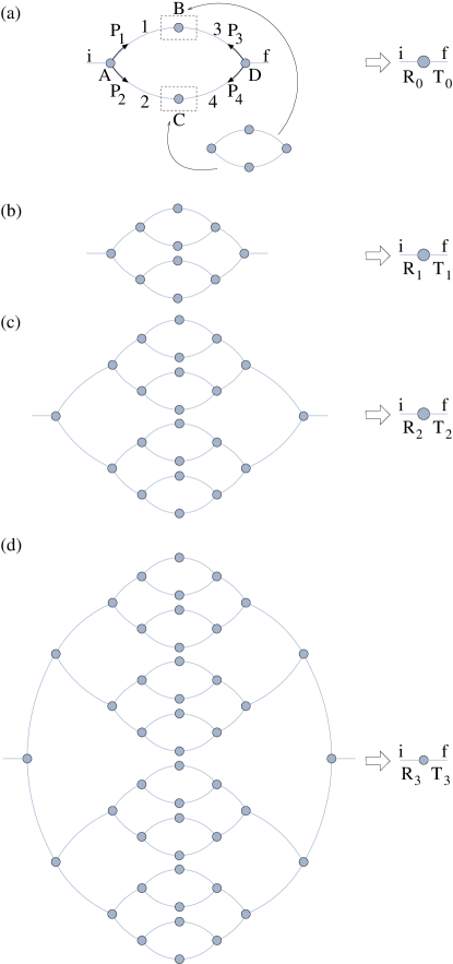
Figure 12: (Color online). Binary tree quantum graphs (attached to leads $i$ and $f$) with different number of recursive compositions $l$. The way a single composition (by insertion) is performed is illustrated in (a). By using the regrouping procedure to calculate the Green’s function, one can reduce the original structure to a simple graph comprising an unique effective vertex linked to two leads (depicted in the right panels). At each level $l$, the rescaled system has the same global transmission $T_{l}$ and reflection $R_{l}$ amplitudes of the corresponding original graph. Here it is shown, (a) the initial basic topology ($l=0$), and (b) $l=1$, (c) $l=2$, and (d) $l=3$, insertions.

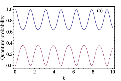
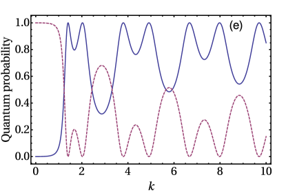
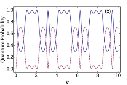
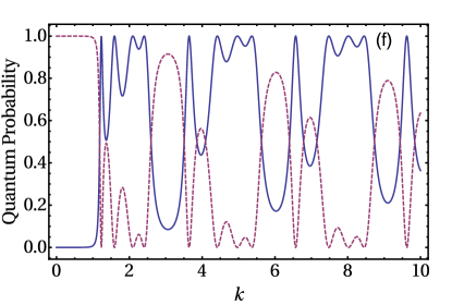
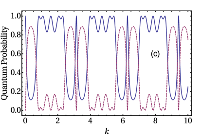
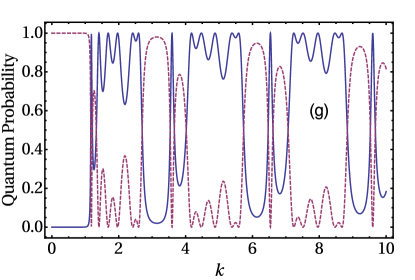
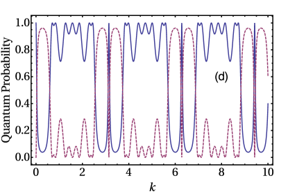
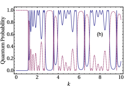
Figure 13: (Color online). The transmission $|T_{l}|^{2}$ (solid line) and reflection $|R_{l}|^{2}$ (dashed) probabilities for the binary trees of Fig. 12. The vertices are generalized $\delta$ interactions of strength (a)-(d) $\gamma=0$ and (e)-(h) $\gamma=1$. All the edges have length $\ell=1$. Here also $\mu=\hbar=1$. The quantum probabilities for the graphs of Fig. 12 (a), (b), (c) and (d) are shown, respectively, in (a) and (e), (b) and (f), (c) and (g) and (d) and (h).

Using the Green’s function method, let us derive the transmission and reflection quantum amplitudes for the basic structure (so level $l=0$) of Fig. 12 (a). In fact, such calculation is similar to that of $r_{I}^{(1)}$ and $t_{I}^{(11,1)}$ for the graph of Fig. 9 (g). By grouping the four vertices $A$, $B$, $C$ e $D$ in a single vertex $l=0$ (right panel of Fig. 12 (a)), the global reflection coefficient $R_{0}$, from $i$ to $i$, is given by (see the left panel of Fig. 12 (a))

$$R_{0}=r_{A}^{(i)}+t_{A}^{(1,i)}\,P_{1}+t_{A}^{(2,i)}\,P_{2}$$ (69)

where

$$\left\{\begin{array}[]{l}P_{1}=r_{B}^{(1)}\,\exp[2ik\ell]\,\left(r_{A}^{(1)}\,P_{1}+t_{A}^{(2,1)}\,P_{2}+t_{A}^{(i,1)}\right)\\ \ \ \ \ \,\,+\,\,t_{B}^{(3,1)}\,\exp[2ik\ell]\,\left(r_{D}^{(3)}\,P_{3}+t_{D}^{(4,3)}\,P_{4}\right)\\ P_{2}=r_{C}^{(2)}\,\exp[2ik\ell]\,\left(r_{A}^{(2)}\,P_{2}+t_{A}^{(1,2)}\,P_{1}+t_{A}^{(i,2)}\right)\\ \ \ \ \ \,\,+\,\,t_{C}^{(4,2)}\,\exp[2ik\ell]\,\left(r_{D}^{(4)}\,P_{4}+t_{D}^{(3,4)}\,P_{3}\right)\\ P_{3}=t_{B}^{(1,3)}\,\exp[2ik\ell]\,\left(r_{A}^{(1)}\,P_{1}+t_{A}^{(2,1)}\,P_{2}+t_{A}^{(i,1)}\right)\\ \ \ \ \ \,\,+\,\,r_{B}^{(3)}\,\exp[2ik\ell]\,\left(r_{D}^{(3)}\,P_{3}+t_{D}^{(4,3)}\,P_{4}\right)\\ P_{4}=t_{C}^{(2,4)}\,\exp[2ik\ell]\,\left(r_{A}^{(2)}\,P_{2}+t_{A}^{(1,2)}\,P_{1}+t_{A}^{(i,2)}\right)\\ \ \ \ \ \,\,+\,\,r_{C}^{(4)}\,\exp[2ik\ell]\,\left(r_{D}^{(4)}\,P_{4}+t_{D}^{(3,4)}\,P_{3}\right).\end{array}\right.$$ (70)

The transmission coefficient $T_{0}$ (from $i$ to $f$) follows from

$$T_{0}=t_{A}^{(1,i)}\,P_{1}+t_{A}^{(2,i)}\,P_{2},$$ (71)

where the $P$’s are given by Eq. (70), but for which we exchange all the indices (including those of the $P$’s) as: $1\leftrightarrow 3$, $2\leftrightarrow 4$, $A\leftrightarrow D$ and $i\leftrightarrow f$. Solving the system (70) we get $R_{0}$ and $T_{0}$. We observe that the reflection (for $f\rightarrow f$) and transmission (for $f\rightarrow i$) are acquired, respectively, from the expressions $R_{0}$ and $T_{0}$ by just applying the above same exchange of indices.

Then, we can substitute the vertices $B$ and $C$ by our basic graph structure, as schematically represented in Fig. 12 (a). This leads to the graph of Fig. 12 (b) (level $l=1$) of quantum amplitudes $R_{1}$ ($i\rightarrow i$) and $T_{1}$ ($i\rightarrow f$). These latter coefficients are exactly those for $R_{0}$ and $T_{0}$, but where in the place of $r_{B}$, $r_{C}$, $t_{B}$ and $t_{C}$ we use the corresponding $R_{0}$ and $T_{0}$. Such process can be repeated any number of times, with $R_{l}$ and $T_{l}$ always directly obtained from $R_{l-1}$ and $T_{l-1}$.

As a numerical example, consider the edges with the same length $\ell=1$ and Dirac $\delta$ interactions of intensity $\gamma$ (for $\gamma=0$ and $\gamma=1$) as the boundary conditions (see Appendix C.1) at all the vertices. For the vertices with $N=2$ edges (say $B$ and $C$) we have $r=\gamma/(ik-\gamma)$ and $t=ik/(ik-2\gamma)$ and for those with $N=3$ (say $A$ and $D$) $r=(2\gamma-ik)/(3ik-2\gamma)$ and $t=2ik/(3ik-2\gamma)$. In Fig. 13 we show the reflection $|R_{l}|^{2}$ ($i\rightarrow i$) and transmission $|T_{l}|^{2}$ ($i\rightarrow f$) probabilities for the basic structure (Fig. 12 (a)) and for the three levels of insertions for the binary tree (Fig. 12 (b)–(d)). As it should be expected, for higher $l$’s the patterns of reflection and transmission, as function of $k$, become much more complex. Also, we do not observe any systematic increasing of $|T_{l}|^{2}$ as $k$ increases because the rich interference behavior – due to the wave propagation along the distinct edges – takes place for any value of $k$.

6.3 Sierpiński-like graphs

One of the many reasons for the interest in self-similar lattices is their utility to model systems which are self-assembled from an original backbone (the motif of the replication), the case of certain complex molecules [209]. Sierpiński graphs are very nice examples of structures which can be recursively generated from a basic building block. They originate from the Sierpiński gasket, a well-known fractal object introduced by Sierpiński in 1915 [210].

Sierpiński graphs have been studied in relation to small-world networks [212]. Also, Sierpiński gaskets have been analyzed in [213, 214], where Neumann-Kirchhoff boundary conditions were considered. However, the most general case of arbitrary reflection and transmission amplitudes for the vertices are still not well explored in the literature.

Here we shall address procedures similar to those of the previous section, allowing one to derive the scattering Green’s function for the Sierpiński graph. We present a schematic method to regroup the multiple stages of the graph (up to stage $n$), leading to the total $R$ and $T$ amplitudes for the whole composition in terms of the basic vertices $A$, $B$, $C$ (Fig. 14) scattering coefficients. But the construction next is not a simple repetition of the binary tree graph calculation. One must take into account that part of the edges change their lengths from one Sierpiński stage to another. This means that in fact $R_{n}$ and $T_{n}$ are not trivial functions of the actual edges lengths at each stage $n$.

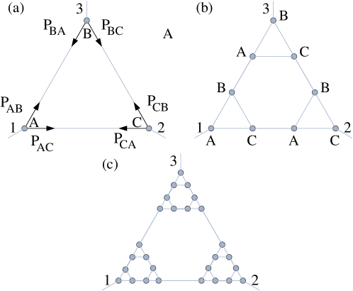
Figure 14: (Color online). Finite Sierpiński graphs with different number $n$ of recursive stages: (a) $n=1$ (the initial $\Delta_{ABC}$ structure, main text), (b) $n=2$, and (c) $n=3$. The $P$’s in (a) represent proper infinite families of scattering paths useful to calculate the Green’s function. The generation of new vertices from (a) to (b) illustrates the elementary transformation to $\Delta_{ABC}$, the basic step leading to the successive graph stages.

In Fig. 14 we show three different stages ($n=1,2,3$) of a Sierpiński graph. The basic step to go from $n$ to $n+1$ involves a transformation in all the fundamental equilateral triangles $\Delta_{ABC}$ of the graph $n$. For instance, starting from $n=1$ (the basic configuration of Fig. 14 (a), with all the three edges of length $\ell_{1}=\ell$), $n=2$ is created by adding two extra vertices to each side of $\Delta_{ABC}$, as illustrated in Fig. 14 (b). To obtain $n=3$, the procedure is repeated for the three $\Delta_{ABC}$ in Fig. 14 (b), leading thus to the 9 triangles $\Delta_{ABC}$ of Fig. 14 (c), and so on and so forth. Note that at the stage $n\ (=1,2,\ldots)$, all the sides of the triangles $\Delta_{ABC}$ have a same length $\ell_{n}=\ell/3^{(n-1)}$.

Since at any stage $n$ the graph always has exactly three semi-infinite leads, the scattering matrix is of order $3$ and given by (see Appendix A)

$$S_{n}=\left(\begin{array}[]{ccc}R_{n}^{(1)}&T^{(1,2)}_{n}&T^{(1,3)}_{n}\\ T^{(2,1)}_{n}&R^{(2)}_{n}&T^{(2,3)}_{n}\\ T^{(3,1)}_{n}&T^{(3,2)}_{n}&R^{(3)}_{n}\end{array}\right).$$ (72)

Above, $R_{n}^{(a)}$ and $T_{n}^{(b,a)}$ are the resulting reflection (from lead $a\ (=1,2,3)$) and transmission (from lead $a$ to lead $b$, with $a\neq b$ and $a,b=1,2,3$) amplitudes for the group of $3^{n}$ vertices constituting the Sierpinński graph at stage $n$ (see Fig. 14).

The Green’s function for the transmission case of the Sierpiński graph of stage $n$ is given by (for $x_{f}$ in lead $b$ and $x_{i}$ in lead $a$)

$$G_{ba}(x_{f},x_{i};k)=\frac{\mu}{i\hbar^{2}k}T_{n}^{(b,a)}\exp[ik(x_{f}+x_{i})].$$ (73)

For the reflection case the Green’s function reads (for $x_{i}$ and $x_{f}$ in lead $a$)

$$G_{aa}(x_{f},x_{i};k)=\frac{\mu}{i\hbar^{2}k}\Big{(}\exp[ik|x_{f}-x_{i}|]+R_{n}^{(a)}\exp[ik(x_{f}+x_{i})]\Big{)}.$$ (74)

For simplicity, we next assume that all the elementary vertices $V=A,B,C$ (Fig. 14 (a)) have the same scattering properties along any edge, thus $r_{V}^{(a)}=r$ and $t_{V}^{(b,a)}=t$. Hence, for all $n$ it holds that $R_{n}^{(a)}=R_{n}$ and $T_{n}^{(b,a)}=T_{n}$. Because so, the specific leads we choose to calculate $R_{n}$ and $T_{n}$ will not alter the final expression. In this way, for $n=1$, Fig. 14 (a), we consider the reflection from lead $2$ and the transmission from lead $1$ to lead $2$, or (recalling that $\ell_{1}$ is just $\ell$)

$$T_{1}(\ell_{1})=t\,(P_{AB}+P_{AC}),\qquad R_{1}(\ell_{1})=r+t\,(P_{CA}+P_{CB}),$$ (75)

where (see Fig. 14 (a))

$$\left\{\begin{array}[]{l}P_{AB}=\exp[ik\ell_{1}]\,(r\,P_{BA}+t\,P_{BC})\\ P_{AC}=\exp[ik\ell_{1}]\,(r\,P_{CA}+t\,P_{CB}+t)\\ P_{BC}=\exp[ik\ell_{1}]\,(r\,P_{CB}+t\,P_{CA}+t)\\ P_{BA}=\exp[ik\ell_{1}]\,(r\,P_{AB}+t\,P_{AC})\\ P_{CA}=\exp[ik\ell_{1}]\,(r\,P_{AC}+t\,P_{AB})\\ P_{CB}=\exp[ik\ell_{1}]\,(r\,P_{BC}+t\,P_{BA})\end{array}\right..$$ (76)

Solving the system of equations in (76), we get the transmission and reflection coefficients of the Sierpiński graph stage $n=1$, Fig. 14 (a), as

$$R_{1}(\ell_{1})=r+\frac{2t^{2}\big{(}r+(t^{2}-r^{2})\exp{[ik\ell_{1}]}\big{)}\exp{[2ik\ell_{1}]}}{\big{(}1-(r+t)\exp{[ik\ell_{1}]}\big{)}\big{(}1+t\exp{[ik\ell_{1}]}+(t^{2}-r^{2})\exp{[2ik\ell_{1}]}\big{)}}$$ (77)

and

$$T_{1}(\ell_{1})=\frac{t^{2}\big{(}1+(t-r)\exp{[ik\ell_{1}]}\big{)}\exp{[ik\ell_{1}]}}{\big{(}1-(r+t)\exp{[ik\ell_{1}]}\big{)}\big{(}1+t\exp{[ik\ell_{1}]}+(t^{2}-r^{2})\exp{[2ik\ell_{1}]}\big{)}}.$$ (78)

Finally, given the system hierarchical character, the scattering coefficients for the stage $n+1$ can be recursively obtained from those of stage $n$. Indeed, from the geometry of the graph formation process, depicted in Fig. 14, and from Eqs. (77) and (78), one concludes after some straightforward reasoning that

$$R_{n+1}(\ell_{n+1})=R_{n}(\ell_{n}/3)+\frac{2[T_{n}(\ell_{n}/3)]^{2}\big{(}R_{n}(\ell_{n}/3)+([T_{n}(\ell_{n}/3)]^{2}-[R_{n}(\ell_{n}/3)]^{2})\exp{[ik\ell/3]}\big{)}\exp{[2ik\ell/3]}}{D_{n}(\ell_{n}/3)}$$ (79)

and

$$T_{n+1}=\frac{[T_{n}(\ell_{n}/3)]^{2}\big{(}1+(T_{n}(\ell_{n}/3)-R_{n}(\ell_{n}/3))\exp{[ik\ell/3]}\big{)}\exp{[ik\ell/3]}}{D_{n}(\ell_{n}/3)},$$ (80)

for

$$D_{n}(L)\equiv\big{(}1-(R_{n}(L)+T_{n}(L))\exp[ikL]\big{)}\,\big{(}1+T_{n}(L)\exp[ikL]+([T_{n}(L)]^{2}-[R_{n}(L)]^{2})\exp[2ikL]\big{)}.$$ (81)

Observe that the above equations correctly account for the reduction by a factor three in the fundamental triangles $\Delta_{ABC}$ edges length of the successive stages of the Sierpiński graph.

Setting $\ell=\ell_{1}=1$ and the same delta point interaction of strength $\gamma$ at all the elementary vertices $A$, $B$, and $C$, we show in Fig. 15 ($\gamma=0$) and Fig. 16 ($\gamma=1$), the behavior of the reflection and transmission coefficients as function of $k$ for the Sierpiński graph stage $n$, up to $n=5$. We notice that as $n$ increases, the system becomes more and more selective to which $k$’s (or equivalently, energies) can be transmitted through the structure. This effect is stronger for $\gamma=1$ (Fig. 16) since then the elementary $r$’s and $t$’s are also $k$-dependent. So, in this respect the Sierpiński graph at the different stages contrasts with the binary tree at different levels, Fig. 13, for which there is not a such filter-like phenomenon.

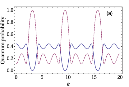
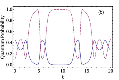
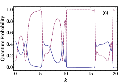
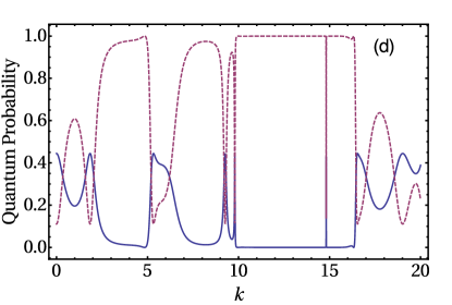
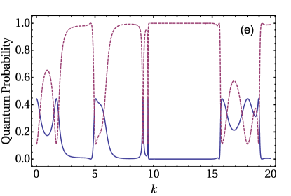
Figure 15: (Color online). The transmission $|T_{n}|^{2}$ (solid line) and reflection $|R_{n}|^{2}$ (dashed) probabilities for the stage $n$ of the Sierpiński graph, Fig. 14. Here $\ell=\ell_{1}=1$ and at any elementary vertex $A$, $B$, and $C$, we assume a same generalized $\delta$ interaction of strength $\gamma=0$. The cases $n=1$, $n=2$, $n=3$, $n=4$, and $n=5$, are displayed, respectively, in (a), (b), (c), (d) and (e).

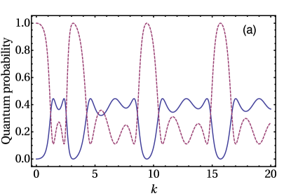
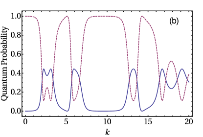
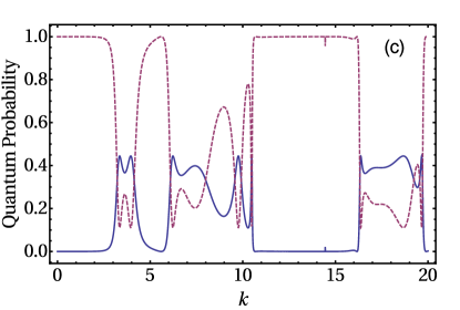
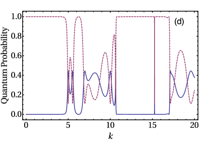
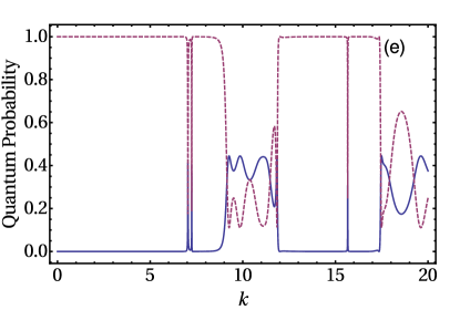
Figure 16: (Color online). The same as in Fig. 15, but for $\gamma=1$.

7 Quasi-bound states in quantum graphs

7.1 Basic aspects

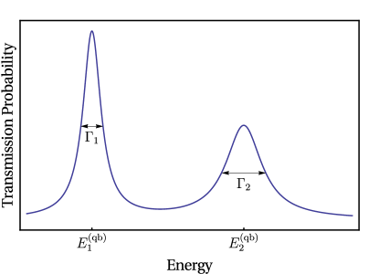
Figure 17: (Color online). Typical profile of the transmission probability as function of energy for a system displaying two quasi-bound states at energies $E_{1}^{(\rm qb)}$ and $E_{2}^{(\rm qb)}$. The quasi-bound states widths, here $\Gamma_{1}$ and $\Gamma_{2}$, are usually defined as the half height widths of the corresponding peaks.

As a last application for the Green’s function approach reviewed so far, we finally consider a context not usually addressed for the present quantum systems (but see [183]): quasi-bound states. For a general treatment of such problems using $G$ – however not discussing quantum graphs – we cite [215].

In quantum mechanics, a quasi-bound state is a type of resonance, associated to the geometry and (local) features of the system potential $V$. Suppose a quantum particle of total energy $E=\hbar^{2}k^{2}/(2\mu)$, whose value is assumed in a certain range $\Sigma_{E}$. Also suppose a region ${\mathcal{V}}$ of the space in which $V$ is attractive or has the generic shape of a well. It might be that the potential cannot confine infinitely the particle to ${\mathcal{V}}$. In other words, for energies $E\in\Sigma_{E}$ the potential $V$ does not support true bound states localized in ${\mathcal{V}}$. However, for specific $E=E^{(\rm{qb})}\in\Sigma_{E}$, $V$ may be able to trap the particle in ${\mathcal{V}}$ during a very long time $\tau$ [216]. Such $\tau$ is called the lifetime of the quasi-bound state of energy $E^{(\rm{qb})}$.

The concept of quasi-bound states is ubiquitous, and has been used to explain a large number of phenomena. For instance, tunneling ionization rates [217], diffraction in time [218], decay of cold atoms in quasi-one-dimensional traps [219], and certain condensed-matter experiments [220], just to mention few examples.

We begin our analysis with the simple linear quantum graph of Fig. 3 (a), Sec. 4.1. It is formed by two vertices, $A$ and $B$, joined together by an edge of length $\ell_{1}$. Each vertex is also attached to a semi-infinite lead. Now, we take for the vertices delta interactions of a same strength $\gamma$. If $\gamma\rightarrow+\infty$, then $r_{A}=r_{B}=-1$ and $t_{A}=t_{B}=0$ (see Sec. 5), which is equivalent to Dirichlet boundary conditions at $A$ and $B$. Then, the graph system becomes equivalent to an infinite square well. In fact, for $k=k_{n}=n\pi/\ell_{1}$ with $n=1,2,3,\dots$ (so, for well determined energies $E_{n}=n^{2}\pi^{2}\hbar^{2}/(2\mu\ell_{1}^{2})$), an acceptable standing solution is $\psi_{1}(x)={\mathcal{C}}\,\sin[k_{n}x]$ along the edge and vanishing $\psi$’s at the leads. This is a proper stationary wave function of infinite lifetime, hence a genuine bound state (in the sense that these $\psi$’s are (not-scattering) eigenstates of the problem Hamiltonian).

Further, if for this same graph we set arbitrary boundary conditions resulting in non-zero transmission amplitude at least for one of the two vertices, the quantum particle initially localized in the edge cannot remain there, eventually it will escape due to tunneling. But as explained above, embedded in the continuous spectrum of $k$ there may exist a discrete set of values $k_{n}^{(\rm{qb})}$ corresponding to the quasi-energies $E_{n}^{(\rm{qb})}=\hbar^{2}{k_{n}^{(\rm{qb})}}^{2}/(2\mu)$ of widths $\Gamma_{n}=\hbar/\tau_{n}$ [222]. A direct way to determine these $k_{n}^{(\rm{qb})}$’s is through a scattering approach. Defining transmission $T(k)$ and reflection $R(k)$ amplitudes for the relevant ${\mathcal{V}}$ region (for contexts where only $R$ is defined, see below), it is a well known fact [221] that $|T(k)|^{2}$ exhibits a pronounced peak for $k$ around $k_{n}^{(\rm{qb})}$. Moreover, the $\Gamma$’s are given by the half height width of the corresponding peaks. Such behavior is schematically illustrated in Fig. 17 (and also concretely observed in some examples in the previous Secs.).

Finally, to frame the problem in terms of the Green’s function formalism, we address $G$ for the graph of Fig. 3 (a) with both $x_{f}$ and $x_{i}$ in lead $i$. Also, to illustrate the situation one can define only a reflection coefficient for the region ${\mathcal{V}}$ (see next), we assume for vertex $B$ boundary conditions leading to a zero transmission amplitude, i.e., the reflection probability from vertex $B$ is exactly 1. In this way we can generally write $r_{B}=\exp[i\phi_{B}]$, for $\phi_{B}(k)$ a wavenumber dependent phase [174]. For $A$, we consider arbitrary boundary condition corresponding to generic $r_{A}$ and $t_{A}$. Note then that the global transmission amplitude $i\rightarrow f$ (crossing $A$–$B$) must be zero because $t_{B}=0$. Hence, any manifestation of a quasi-bound state should be identified in the phase of $R_{ii}(k)=\exp[i\phi_{R}(k)]$.

Following the convention that $0\leq x<+\infty$ in lead $i$ (with the origin at $A$), we have

$$G_{ii}(x_{f},x_{i};k)=\frac{\mu}{i\hbar^{2}k}\left(\exp[ik|x_{f}-x_{i}|]+R_{ii}(k)\,\exp{[ik(x_{f}+x_{i})]}\right),$$ (82)

where $R_{ii}$ is easily derived from the previous sums over paths construction, or (already setting $r_{B}=\exp[i\phi_{B}]$)

$$R_{ii}(k)=r_{A}^{(i)}(k)+\frac{t_{A}^{(1,i)}(k)\,t_{A}^{(i,1)}(k)\,\exp{[i\,(2k\ell_{1}+\phi_{B}(k))]}}{1-r_{A}^{(1)}(k)\,\exp{[i\,(2k\ell_{1}+\phi_{B}(k))]}}.$$ (83)

Using the relations in Eq. (112) for the vertex $A$ quantum amplitudes $r_{A}$ and $t_{A}$, it is a little tedious but straightforward to prove that $R_{ii}\,{R_{ii}}^{*}=1$. So, as previously mentioned we can write $R_{ii}(k)=\exp[i\phi_{R}(k)]$, with $\phi_{R}(k)$ coming from Eq. (83).

The natural question now is how to characterize a quasi-bound state from the function $\phi_{R}(k)$. This is a textbook analysis [222], but answered next by means of a very simple heuristic argument. The system wave function, with $x$ in lead $i$, is (for ${\mathcal{N}}$ a proper normalization constant)

$$\psi(x)={\mathcal{N}}\,\Big{\{}\exp{[-ikx]}+R_{ii}(k)\,\exp{[+ikx]}\,\Big{\}}={\mathcal{N}}\,\Big{\{}\exp{[-ikx]}+\exp{[+i\,(kx+\phi_{R}(k))]}\,\Big{\}}.$$ (84)

It represents the scattering process of plane wave incoming from lead $i$, being scattered at the graph region $A$–$B$, and then being reflected back to lead $i$. Observe that if for a $k=k^{(\rm{qb})}$

$$\phi_{R}(k^{(\rm{qb})})=(2m+1)\,\pi,$$ (85)

with $m=0,1,\ldots$, Eq. (84) yields $\psi(x)\propto\sin[k^{(\rm{qb})}\,x]$. Although here not a real bound state, this is exactly the sine-type of solution for the edge region – thus similar to a stationary standing wave – in the already discussed case the graph is equivalent to an infinite square well. Therefore, the quasi-bound wavenumber must be those $k=k^{(\rm{qb})}$ verifying Eq. (85). The quasi-bound state width is related to a $\Delta k$ around $k^{(\rm{qb})}$ for which $\phi_{R}$ mod $2\pi$ is close enough to $\pi$.

At this point, it should be clear the benefits of the Green’s function method to treat quantum graphs quasi-bound states. On the one hand, the behavior of transmission and reflection probabilities is a direct route to determine the quasi-bound energies. On the other hand, the Green’s function is a very appropriate tool to calculate such quantities, especially for involving topologies. Furthermore, $G$ can be used to obtain transition amplitudes to and from specific parts of a graph, allowing a precise selection of the region of interest ${\mathcal{V}}$. In the following we will discuss recurrence protocols to calculate global $R$ and $T$ for different quantum graphs, also illustrating how to identify the quasi-bound states from such expressions. We should mention that most of the procedures explained in details below have been developed with distinct purposes in different previous works [150, 192, 137, 77, 183] and are somehow related to the general idea of the transfer matrix method [223].

7.2 Recurrence formulas for the reflection and transmission coefficients

Next we discuss the derivation of recurrence formulas for the quantum graphs global transmission and reflection amplitudes by means of the present sum over scattering paths technique. For convenience, in the following we address only linear graphs (for the more general case, see Sec. 7.4).

So, consider the linear open quantum graph in Fig. 18, composed by a left semi-infinite lead $i$ and vertices named $l\ (=1,2,\ldots,N)$. Along the lead, the spatial coordinate $x$ ranges from $+\infty$ to 0 (with the origin at the vertex 1). For the edge $e_{l}$ (between vertices $l$ and $l+1$), $x$ goes from 0 (at vertex $l$) to $\ell_{l}$ (at vertex $l+1$).

From the simplification procedures of Sec. 4.2, we can get the Green’s function for the case where $x_{i}$ is in the lead $i$ and $x_{f}$ is in the edge $e_{l}$ (see Fig. 18) as

$$G_{li}(x_{f},x_{i};k)={} \frac{\mu}{i\hbar^{2}k}\frac{T_{(1,l)}^{(+)}}{\left(1-R_{(1,l)}^{(-)}\,R_{(l+1,N)}^{(+)}\,\exp{[2ik\,\ell_{l}]}\right)}\Big{(}\exp[ik\,(x_{f}+x_{i})]+R_{(l+1,N)}^{(+)}\,\exp[ik\,(2\ell_{l}-x_{f}+x_{i})]\Big{)}.$$ (86)

In the above, for $l_{b}\geq l_{a}$, the subscript ($l_{a},l_{b}$) indicating the full block of vertices and edges from $l_{a}$ to $l_{b}$, and the superscript $(+/-)$ meaning incoming from the left/right, then $T_{(l_{a},l_{b})}^{(\pm)}$ ($R_{(l_{a},l_{b})}^{(\pm)}$) represents the global transmission (reflection) coefficient across (from) such $l_{a}$—$l_{b}$ graph block. Note that $T_{l,l}^{(\pm)}=t_{l}^{(\pm)}$ and $R_{l,l}^{(\pm)}=r_{l}^{(\pm)}$, for $t_{l}$ and $r_{l}$ the quantum amplitudes of the individual vertex $l$.

Figure 18: (Color online). A linear graph composed by a semi-infinite lead $i$ (at the left) attached to a series of $N$ simply connected vertices. This structure allows quasi-bound states.

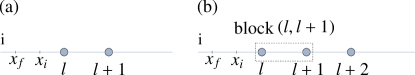
Figure 19: (Color online). Linear graphs with (a) two and (b) three simply connected vertices attached to left and right leads. In (b) it is exemplified the construction process of a block structure.

These $T_{(l_{a},l_{b})}^{(\pm)}$ and $R_{(l_{a},l_{b})}^{(\pm)}$ are recursively obtained in terms of the reflection and transmission coefficients of each individual vertex. To see how, consider the graph composed of two vertices, $l$ and $l+1$, an edge $e_{l}$, and two, left and right, leads. We also assume both $x_{i},x_{f}$ in the left lead, Fig. 19 (a). Performing the sum over all scattering paths, the Green’s function for the graph in Fig. 19 (a) reads

$$G_{ii}(x_{f},x_{i};k)={} \frac{\mu}{i\hbar^{2}k}\Biggl{(}\exp[ik|x_{f}-x_{i}|]+r^{(+)}_{l}\,\exp[ik(x_{f}+x_{i})]$$

$$+\frac{t^{(+)}_{l}\,r^{(+)}_{l+1}\,t^{(-)}_{l}\,\exp{[2ik\ell_{l}]}}{1-r^{(-)}_{l}\,r^{(+)}_{l+1}\,\exp[2ik\ell_{l}]}\exp{[ik(x_{f}+x_{i})]}\Biggr{)}.$$ (87)

From the above expression it is easy to identify a global reflection coefficient from the left of block $(l,l+1)$, Fig. 19 (b), or

$$R^{(+)}_{(l,l+1)}=r^{(+)}_{l}+\frac{t^{(+)}_{l}\,r^{(+)}_{l+1}\,t^{(-)}_{l}\,\exp[2ik\ell_{l}]}{1-r^{(-)}_{l}\,r^{(+)}_{l+1}\,\exp{[2ik\ell_{l}]}}.$$ (88)

Similarly, calculating $G$ for $x_{i},x_{f}$ in the right lead, we also can identify a global reflection coefficient from the right of this same block, given by

$$R^{(-)}_{(l,l+1)}=r^{(-)}_{l+1}+\frac{t^{(-)}_{l+1}\,r^{(-)}_{l}\,t^{(+)}_{l+1}\,\exp[2ik\ell_{l}]}{1-r^{(-)}_{l}\,r^{(+)}_{l+1}\,\exp{[2ik\ell_{l}]}}.$$ (89)

Now, considering the case in which $x_{i}$ ($x_{f}$) is in the left (right) lead, then

$$G_{fi}(x_{f},x_{i};k)=\frac{\mu}{i\hbar^{2}k}\frac{t^{(+)}_{l}\,t^{(+)}_{l+1}\,\exp[ik\ell_{l}]}{\left(1-r^{(-)}_{l}\,r^{(+)}_{l+1}\,\exp{[2ik\ell_{l}]}\right)}\exp[ik(x_{f}+x_{i})],$$ (90)

naturally yielding

$$T^{(+)}_{(l,l+1)}=\frac{t^{(+)}_{l}\,t^{(+)}_{l+1}\,\exp{[ik\ell_{l}]}}{1-r^{(-)}_{l}\,r^{(+)}_{l+1}\,\exp{[2ik\ell_{l}]}}.$$ (91)

Finally, from $G$ for $x_{i}$ ($x_{f}$) in the right (left) lead, one finds

$$T^{(-)}_{(l,l+1)}=\frac{t^{(-)}_{l}\,t^{(-)}_{l+1}\,\exp{[ik\ell_{l}]}}{1-r^{(-)}_{l}\,r^{(+)}_{l+1}\,\exp{[2ik\ell_{l}]}}.$$ (92)

With proper substitutions, the above Eqs. (88), (89), (91), and (92) constitute then the basic generating expressions to obtain $R$ and $T$ for an arbitrary number of vertices in a linear graph. To exemplify this, let us assume a third vertex $l+2$, as shown in Fig. 19 (b). For $x_{i},x_{f}$ in the left lead, we can suppose $l$—$(l+1)$ forming a block of coefficients $R_{(l,l+1)}^{(\pm)}$ and $T_{(l,l+1)}^{(\pm)}$ (see Fig. 19 (b)). Hence, by mapping the vertex $l$, the vertex ${l+1}$ and the edge $e_{l}$ of Fig. 19 (a) into, respectively, the $l$—$(l+1)$ block, the vertex $l+2$, and the edge $e_{l+1}$ of Fig. 19 (b), we can directly infer from Eq. (88) that

$$R^{(+)}_{(l,l+2)}=R^{(+)}_{(l,l+1)}+\frac{T^{(+)}_{(l,l+1)}\,r^{(+)}_{l+2}\,T^{(-)}_{(l,l+1)}\,\exp[2ik\ell_{l+1}]}{1-R^{(-)}_{(l,l+1)}\,r^{(+)}_{l+2}\,\exp[2ik\ell_{l+1}]}.$$ (93)

To close, based on the previous examples, one can readily generalize the above results for a block $(l,l+n)$ of $n+1$ vertices, obtaining the following recursive relations

$$R^{(+)}_{(l,l+n)}=R^{(+)}_{(l,l+n-1)}+\frac{T^{(+)}_{(l,l+n-1)}\,r^{(+)}_{l+n}\,T^{(-)}_{(l,l+n-1)}\,\exp[2ik\ell_{l+n-1}]}{1-R^{(-)}_{(l,l+n-1)}\,r^{(+)}_{l+n}\,\exp[2ik\ell_{l+n-1}]},$$ (94)

$$R^{(-)}_{(l,l+n)}=r^{(-)}_{l+n}+\frac{t^{(-)}_{l+n}\,R^{(-)}_{(l,l+n-1)}\,t^{(+)}_{l+n}\,\exp[2ik\ell_{l+n-1}]}{1-R^{(-)}_{(l,l+n-1)}\,r^{(+)}_{l+n}\exp[2ik\ell_{l+n-1}]},$$ (95)

$$T^{(\pm)}_{(l,l+n)}=\frac{T^{(\pm)}_{(l,l+n-1)}\,t^{(\pm)}_{l+n}\exp[ik\ell_{l+n-1}]}{1-R^{(-)}_{(l,l+n-1)}\,r^{(+)}_{l+n}\exp[2ik\ell_{l+n-1}]},$$ (96)

7.3 Green’s function as a transition probability amplitude and the determination of quasi-bound states

Once we now know the recurrence formulas for the scattering coefficients of a linear quantum graph, we can return to the Green’s function in Eq. (86). But first we shall recall that $G(x_{f},x_{i};k)$ can be generally interpreted as the transition probability amplitude for a particle (of fixed energy $E=\hbar^{2}k^{2}/(2\mu)$) initially in $x_{i}$ to get to $x_{f}$ [181]. Thus, the overall multiplicative term in Eq. (86), namely,

$$\mathcal{A}_{i,l}(k)=\frac{T_{1,l}^{(+)}(k)}{1-R_{1,l}^{(-)}(k)\,R_{l+1,N}^{(+)}(k)\,\exp{[2ik\ell_{j}]}},$$ (97)

represents the probability amplitude for a particle (of wavenumber $k$) to leave the left semi-infinite lead $i$ and to tunnel to the edge $e_{l}$.

So, if the graph supports a quasi-bound state totally or partially localized in $e_{l}$, an incident wave (from lead $i$) with $k$ close to the corresponding quasi-bound state $k^{(\rm{qb})}$ value should have a very high probability to be transmitted to the edge $e_{l}$ region. In this way, the plot of $|\mathcal{A}_{i,l}|^{2}$ as function of $k$ (or likewise of $E$) should display peaks centered at the correct $E^{(\rm qb)}$’s, as schematically depicted in Fig. 17. Moreover, such peaks widths at half height would correspond to the $\Gamma$’s.

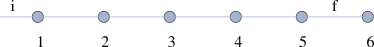
Figure 20: (Color online). The graph of Fig. 18 for $N=6$ and all edges of the same length $\ell_{l}=\ell$. The vertex 6 is the system ‘dead end’, for which is assumed either Dirichlet or Neumann boundary conditions. The other vertices are delta interactions of strength $\gamma$.

As an example, consider the linear open graph with six vertices of Fig. 20, where the last vertex 6 is a ‘dead end’. We suppose for all edges $\ell_{l}=\ell=1$ and for the vertices 1 to 5 generalized $\delta$ interactions of a same strength $\gamma$. However, for vertex 6 we assume either Dirichlet (so $r_{6}^{(+)}=-1$) or Neumann (so $r_{6}^{(+)}=+1$) boundary conditions. For two values of the delta intensity, $\gamma=1$ and $\gamma=2$, and for $l$ varying from 1 to 5, we plot in Figs. 21 and 22 the quantity $|\mathcal{A}_{i,l}|^{2}$ as function of $k$ for, respectively, the Dirichlet and Neumann boundary conditions at vertex 6.

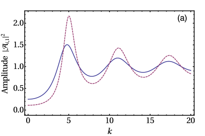
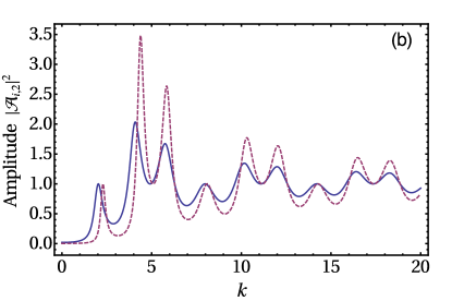
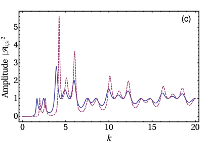
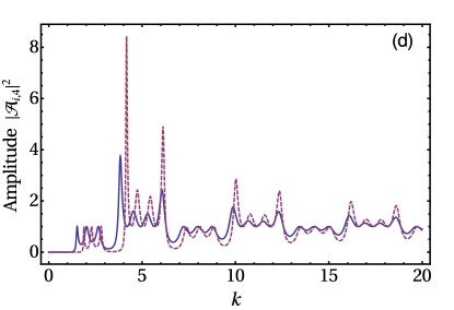
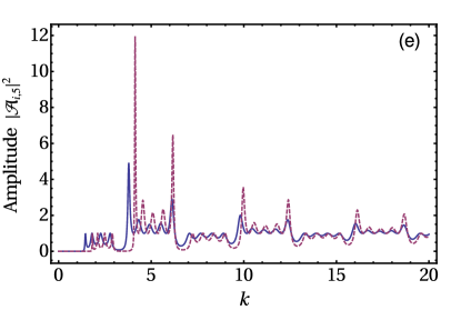
Figure 21: (Color online). The transition probability $|\mathcal{A}_{i,l}|^{2}$, Eq. (97), as a function of $k$ for the graph of Fig. 20 with the Dirichlet boundary condition at the vertex 6 (so, $r_{6}^{(+)}=-1$). The $l$’s are (a) 1, (b) 2, (c) 3, (d) 4, and (e) 5. The solid (dashed) line is for $\gamma=1$ ($\gamma=2$). Here $\ell=1$.

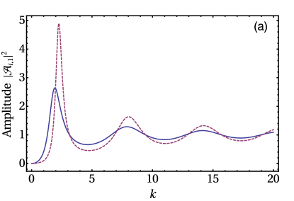
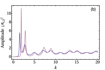
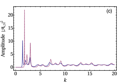
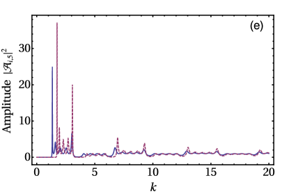
Figure 22: (Color online). The same as in Fig. (21), but for the Neumann boundary condition at the vertex 6 (so, $r_{6}^{(+)}=+1$).

From the plots in Figs. 21 and 22 we see that the analysis of the $\mathcal{A}_{i,l}$’s for distinct $l$’s renders a much more detailed information than just to examine the system global reflection coefficient $R_{ii}=\exp[i\phi_{R}(k)]$. For instance, for the $r_{6}^{(+)}=-1$ case, Fig. 21, and when $\gamma=2$, it is clear the existence of a $k^{(\rm{qb})}\approx 4.2$. Indeed, we see peaks around this wavenumber value for fairly all the $l$’s. Nevertheless, they are much higher and narrower for $l=4,5$. Hence, such quasi-bound state must be much more localized in these two edges. Another observed feature is that the quasi-bound states are longer-lived for $\gamma=2$ than for $\gamma=1$ (compare the heights and widths of the peaks in the two situations). This is simple to understand: a delta interaction of greater strength is more efficient in trapping an initially localized state. Finally, from the general trends in Figs. 21 and 22 we also can conclude that it is the Neumann boundary condition (at the ‘dead end’ vertex 6) which is able to create quasi-bound states of longer $\tau$’s.

7.4 Quasi-bound state in arbitrary graphs

Inspecting the expression for $\mathcal{A}_{i,l}$ in Eq. (97) (as well as other similar formulas along this review), we conclude that typical transitions amplitudes between parts of a quantum graph – in which $x_{i}$ is in a lead $i$ and $x_{f}$ is in an edge $e_{l}$ – are given by

$$\mathcal{A}_{i,l}=\frac{T_{i,l}}{1-R_{\rm{right}}\,R_{\rm{left}}\,\exp[2ik\ell_{l}]}.$$ (98)

The numerator is a transmission coefficient, corresponding to the graph region between $x_{i}$ (in the lead $i$) and $x_{f}$ (in the edge $l$). In the denominator, $R_{\rm{right}}$ ($R_{\rm{left}}$) is the global reflection coefficient for a part of the graph, so to speak, to the ‘right’ of edge $l+1$ (to the ‘left’ of vertex $l$, between $x_{i}$ and the vertex $l$). Note also that the term in the denominator is associated with eventual energy eigenvalues [224, 152], and in general can be derived from a sum over periodic orbits in the graph (i.e., scattering paths leaving and arriving at the same edge $l$) [137, 38, 39].

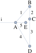
Figure 23: (Color online). Example of an open quantum graph, whose a modified version has been studied in [137].

Therefore, Eq. (98) is not restricted to a linear graph, and in fact should work for any topology (provided one properly defines and constructs the $R$’s and $T$). As an example, consider the structure in Fig 23. Such graph can display interesting features if one assumes different boundary conditions at each vertex and distinct lengths for each edge (see [137]). But here we restrict the discussion to generalized delta point interactions of a same strength $\gamma$ at the vertices $A$, $B$, $C$, $D$, and either Dirichlet or Neumann boundary conditions (see previous section) at the vertex $E$. Also, we suppose all the edges with the length $\ell=1$. So, due to symmetry, the edges 1 and 4 and 2 and 3 must present similar scattering properties and we can focus just on the inequivalent amplitudes $\mathcal{A}_{i,1}(k)$, $\mathcal{A}_{i,2}(k)$, and $\mathcal{A}_{i,5}(k)$. Using Eq. (98) and the appropriate corresponding reflection and transmission quantum amplitudes for the graph of Fig. 23, we show in Fig. 24 the behavior of the modulus square of these three quantities as function of $k$ for the Dirichlet and Neumann boundary conditions at $E$ and the delta interactions strength value $\gamma=0.5$ and $\gamma=1$.

Because the graph distinct geometric characteristics, when compared to the simpler linear case (Fig. 20), we do observe here a richer profile of quasi-bound states. Also, the distinct boundary conditions at $E$ considerably change the positions and sizes of the $E^{(\rm{qb})}$ peaks (this is a same sort of sensibility also found for the transmission probabilities for the related graph studied in [137]). Finally, in general the peaks are higher and narrower, so longer-lived, for the greater value of $\gamma$ ($\gamma=1$).

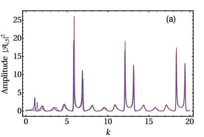
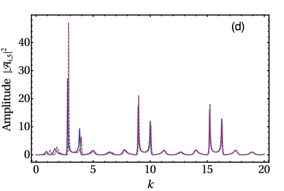
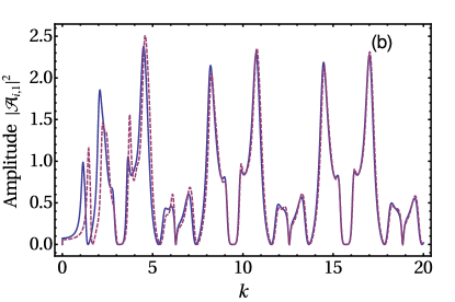
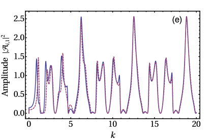
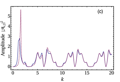
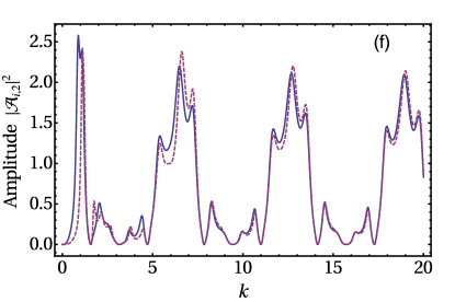
Figure 24: (Color online). Behavior of $|\mathcal{A}_{i,l}|^{2}$ as function of $k$ (calculate from Eq. (98)) for the graph of Fig. 23 and $l=1,2,5$. The vertices $A$, $B$, $C$, and $D$, are generalized delta interactions of strength $\gamma$, with $\gamma=0.5$ (solid) and $\gamma=1$ (dashed) lines. The boundary conditions at vertex $E$ are Dirichlet’s (so, $r_{E}=-1$) in (a)–(c) and Neumann’s (so, $r_{E}=1$) in (d)–(f). All edges have the same length $\ell=1$.

8 Conclusion

The discussions throughout this article have highlighted the usefulness of graphs to study some fundamental theoretical aspects of quantum mechanics as well as to model different phenomena associated to quantum wave-like behavior. But despite the conceptual simplicity of these systems, the calculation of their quantum properties might demand sophisticated and involving methods [139]. Further, certain standard mathematical procedures may require modifications when applied to a graph structure, as to obtain the Green’s function from the Krein’s resolvent formula [138].

Since the Green’s function is one of the most powerful techniques to solve quantum systems [135], in this review we have specifically considered such approach to address finite open and closed undressed quantum graphs of any topology. We have so discussed a physically appealing procedure to construct $G$, summarized in the Eq. (13): the exact Green’s function given as a sum over all the possible scattering “classical” paths (sp) along the edges, for which local quantum effects are taking into account through reflections and transmissions amplitudes defined at the vertices (constituting thus the scatterers centers). Then, the present Green’s function method somehow generalizes the Kirchhoff’s quantum rules [134] by ascribing a general scattering matrix to each vertex of the quantum graph.

In particular, we have described in details recursive ways to sum up all the sp’s contributions to $G$. Basically, they rely on two simplification schemes: (a) to regroup infinite many paths into a single trajectory family; and (b) to divide a larger graph into smaller pieces, to derive for each piece a global scattering matrix, and finally to compose all the pieces back together. As concrete examples, certain representative quantum graphs commonly found in the literature have been considered, as the cube, binary tree and Sierpiński-like structures.

The protocols outlined here could likewise be applied to dressed quantum graphs if the potentials along the edges decay at least exponentially [225]. In fact, in this case very good analytical approximations for the Green’s function can be derived [151, 152]. But then, besides the vertices quantum amplitudes, it is also necessary to consider the potentials reflection and transmission coefficients and to compute the classical actions for a particle under these potentials. Furthermore, a close related class of systems, namely, scattering quantum walks, can be treated exactly in the same fashion. As shown in [77, 78], the exact Green’s function – written as a sum over sp’s – allows to identify the precise paths responsible for distinct effects, like the ones resulting in the super-diffusion observed in quantum walks.

Finally, a very interesting application for Green’s functions (and in the context of open quantum graphs, eventually difficult by other means) is to search for possible quasi-bound states. We have illustrated how to do, moreover analyzing the influence of few different boundary conditions at the vertices in setting the quasi-energies and corresponding widths.

We hope that this review, discussing exact closed analytic expressions for the Green’s functions of quantum graphs, can become a helpful guide to all those interested in this diverse and conceptually and phenomenologically so rich class of systems.

9 Acknowledgments

FMA would like to thank Simone Severini and Sougato Bose at University College London for the hospitality extended during the period this manuscript was finished. Support is acknowledge from CNPq for researcher grants. FMA also thanks CNPq for grants No. 460404/2014-8 (Universal) and 206224/2014-1 (PDE).

A The most general point interaction conserving probability flux as a quantum graph vertex

A.1 The usual case: the line

The probability density flux in the usual 1D quantum mechanics reads (here for $\hbar=\mu=1$)

$$j(x)=\frac{1}{2i}[\psi^{*}(x)\psi^{\prime}(x)-\psi(x)\psi^{\prime*}(x)].$$ (99)

Thus, if we define ($\psi^{\prime}(x)\equiv d\psi(x)/dx$)

$$\Phi(x)=\left(\begin{array}[]{c}\psi(x)\\ \psi^{\prime}(x)\end{array}\right),$$ (100)

and

$$J=\left(\begin{array}[]{cc}0&1\\ -1&0\end{array}\right),$$ (101)

$j(x)$ can be written in a complex symplectic-like form as

$$j(x)=\frac{1}{2i}\Phi^{\dagger}(x)\,J\,\Phi(x).$$ (102)

Now, suppose a free particle of energy $E=k^{2}/2$ on the line ($-\infty<x<+\infty$), obeying to $-d^{2}\psi(x)/dx^{2}=k^{2}\psi(x)$ for $x\neq 0$. At $x=0$ we assume a point interaction. Since, by definition, the range of action of such kind of potential is zero, its only effect is to set a specific BC for the wave function $\psi(x)$ at $x=0$. Thus, the most general point potential corresponds to the most general linear boundary condition, represented by

$$\Phi(0^{+})=\Gamma\,\Phi(0^{-}),$$ (103)

with

$$\Gamma=\omega\left(\begin{array}[]{cc}a&b\\ c&d\end{array}\right).$$ (104)

For example, for the common delta function potential $\gamma\,\delta(x)$ (so, with $\gamma$ being the strength), the parameters are $a=d=\omega=1$, $b=0$, and $c=\gamma$.

Using the Eqs. (102) and (103), we have

$$j(0^{+})=\frac{1}{2i}\Phi^{\dagger}(0^{-})\,\Gamma^{\dagger}\,J\,\Gamma\,\Phi(0^{-}).$$ (105)

If we impose $j(0^{+})=j(0^{-})$, it follows that $\Gamma^{\dagger}\,J\,\Gamma=J$, yielding

$$ad-bc=1,\ a,b,c,d\ \mbox{real numbers and}\ |\omega|=1.$$ (106)

Therefore, the most general point interaction consistent with flux conservation is characterized by Eq. (103), with $\Gamma$ given by Eqs. (104) and (106).

Next, to consider a ${\mathcal{S}}$ matrix formalism [194], suppose typical plane wave scattering solutions (of wavenumber $k$). The incoming and outgoing parts of the state should then be related through

$$\left(\begin{array}[]{c}\psi_{k}^{(\mbox{\scriptsize out})}(0^{-})\\ \psi_{k}^{(\mbox{\scriptsize out})}(0^{+})\end{array}\right)={\mathcal{S}}(k)\left(\begin{array}[]{c}\psi_{k}^{(\mbox{\scriptsize in})}(0^{-})\\ \psi_{k}^{(\mbox{\scriptsize in})}(0^{+})\end{array}\right).$$ (107)

Probability conservation at the origin,

$$|\psi_{k}^{(\mbox{\scriptsize in})}(0^{-})|^{2}+|\psi_{k}^{(\mbox{\scriptsize in})}(0^{+})|^{2}=|\psi_{k}^{(\mbox{\scriptsize out})}(0^{-})|^{2}+|\psi_{k}^{(\mbox{\scriptsize out})}(0^{+})|^{2},$$ (108)

inserted into Eq. (107) leads to ${\mathcal{S}}(k){\mathcal{S}}^{\dagger}(k)={\mathcal{S}}^{\dagger}(k){\mathcal{S}}(k)=\mathbf{1}$, i.e., ${\mathcal{S}}$ is unitary. Furthermore, making in Eq. (107) the substitution $k\rightarrow-k$, we can write

$$\left(\begin{array}[]{c}\psi_{-k}^{(\mbox{\scriptsize in})}(0^{-})\\ \psi_{-k}^{(\mbox{\scriptsize in})}(0^{+})\end{array}\right)={\mathcal{S}}^{\dagger}(-k)\left(\begin{array}[]{c}\psi_{-k}^{(\mbox{\scriptsize out})}(0^{-})\\ \psi_{-k}^{(\mbox{\scriptsize out})}(0^{+})\end{array}\right).$$ (109)

But $k\rightarrow-k$ inverts the flux direction, physically implying in $\psi^{(\mbox{\scriptsize in})}\leftrightarrow\psi^{(\mbox{\scriptsize out})}$. So, given such in-out exchange in Eq. (109) and once the relation between incoming and outgoing wave function components is always set in the form of Eq. (107), we must have ${\mathcal{S}}(k)={\mathcal{S}}^{\dagger}(-k)$.

For any arbitrary point interaction, we can write the scattering solutions $\psi_{k}^{(\pm)}(x)$ assuming a plane wave, of wavenumber $k$, incident either from the left $(+)$ or right $(-)$, so that (${\mathcal{N}}=1/\sqrt{2\pi}$)

$$\psi_{k}^{(\pm)}(x)={\mathcal{N}}\times\left\{\begin{array}[]{ll}\exp{[\pm ikx]}+R^{(\pm)}(k)\exp{[\mp ikx]},&x\lessgtr 0\\ T^{(\pm)}(k)\exp{[\pm ikx]},&x\gtrless 0.\end{array}\right.$$ (110)

Observing that $\exp{[\pm ikx]}$ are the incoming and the terms involving $R$ and $T$ are the outgoing parts of the above full scattering states, one gets that arbitrary linear combinations of $\psi_{k}^{(+)}$ and $\psi_{k}^{(-)}$ results, from Eq. (107), in

$${\mathcal{S}}(k)=\left(\begin{array}[]{cc}R^{(+)}(k)&T^{(-)}(k)\\ T^{(+)}(k)&R^{(-)}(k)\end{array}\right).$$ (111)

Now, imposing ${\mathcal{S}}\,{\mathcal{S}}^{\dagger}={\mathcal{S}}^{\dagger}\,{\mathcal{S}}=\mathbf{1}$ and ${\mathcal{S}}(k)={\mathcal{S}}^{\dagger}(-k)$ to Eq. (111), ones finds that

$$|{R}|^{2}+|{T}|^{2}=1,\qquad{{R}^{(+)}}^{*}{T}^{(\pm)}+{{T}^{(\mp)}}^{*}{R}^{(-)}=0,$$

$${{R}^{(\pm)}}^{*}(k)={R}^{(\pm)}(-k),\qquad{{T}^{(\pm)}}^{*}(k)={T}^{(\mp)}(-k).$$ (112)

These are the basic conditions to assure proper features for the scattering solutions in quantum mechanics [194], e.g., orthonormalization, flux conservation, and the existence of the scattering inverse problem. If, furthermore, one also requires time-reverse invariance – what we are not imposing in this work – then ${T}^{(+)}={T}^{(-)}$.

Finally, to establish a full correspondence between the two approaches, the boundary condition treatment and the ${\mathcal{S}}$ matrix formalism, let us assume Eq. (103) (with Eq. (106)) for the states in Eq. (110). Thus [192]

$${R}^{(\pm)}(k)=\frac{c\pm ik(d-a)+bk^{2}}{-c+ik(d+a)+bk^{2}},\ \ {T}^{(\pm)}(k)=\frac{2ik\omega^{\pm 1}}{-c+ik(d+a)+bk^{2}}.$$ (113)

It is easy to verify that the quantum amplitudes in Eq. (113) satisfies all the fundamental requirements in Eq. (112) [192]. Hence, up to a global phase $\omega$, the problem is likewise specified from the parameters $a,b,c$ and $d$ or from the coefficients $R^{(\pm)}$ and $T^{(\pm)}$. Thus, the two approaches are completely equivalent and arbitrary point interactions can be defined entirely in terms of their $\mathcal{S}$ matrix (for a more detailed analysis, see, e.g., [187]).

A.2 A point interaction in 1D for multiple directions: a star graph topology

The above prescription for the line is directly extended to the more general case. To see how, first note that in the 1D case, a zero-range potential at the origin divides the interval $-\infty<x<+\infty$ into two semi-infinite lines. Thus, from the identification $x_{1}=-x$ and $x_{2}=+x$, the left ($-\infty<x<0$) and right ($0<x<+\infty$) regions could be represented by $0\leq x_{1}\leq+\infty$ and $0\leq x_{2}\leq+\infty$. Hence, in a quantum graph framework, the system topology is that of a single vertex joining two leads. Also, the original nomenclature $0^{+}$ ($0^{-}$) now becomes $x_{2}=0$ ($x_{1}=0$), indicating that we are considering the vertex but from the right (left) side, i.e., at the beginning of lead 2 (1).

A zero-range potential located at 0 and attached to $N=|E(\Gamma)|$ semi-infinite lines constitutes a star graph-like topology, depicted in Figure 1(c). Along each lead $s$ (with $s=1,2,\ldots,N$) the spatial coordinate $x_{s}$ ranges from 0 to $+\infty$ and $\psi_{k}^{(\mbox{\scriptsize in})}(x_{s})$ and $\psi_{k}^{(\mbox{\scriptsize out})}(x_{s})$ denote, respectively, incoming and outgoing $k$ plane wave states. In this case, the equivalent of Eqs. (107) and (109) read

$$\Psi_{k}^{(\mbox{\scriptsize out})}(0)={\mathcal{S}}(k)\,\Psi_{k}^{(\mbox{\scriptsize in})}(0)\ \ \mbox{and}\ \ \Psi_{-k}^{(\mbox{\scriptsize in})}(0)={\mathcal{S}}^{\dagger}(-k)\,\Psi_{-k}^{(\mbox{\scriptsize out})}(0),$$ (114)

with $\Psi$ a $N$-components column vector (naturally extending the $2$-components for the line) and ${\mathcal{S}}(k)$ a $N\times N$ scattering matrix, whose element ${\mathcal{S}}^{(sr)}(k)$ yield the quantum transition amplitude to go from lead $r$ to lead $s$ for a state of wave number $k$. Probability conservation and moment inversion reciprocity, namely,

$${\Psi_{k}^{(\mbox{\scriptsize out})}(0)}^{\dagger}\,\Psi_{k}^{(\mbox{\scriptsize out})}(0)={\Psi_{k}^{(\mbox{\scriptsize in})}(0)}^{\dagger}\,\Psi_{k}^{(\mbox{\scriptsize in})}(0)\ \mbox{and}\ k\leftrightarrow-k\Longleftrightarrow\ \Psi^{(\mbox{\scriptsize out})}\leftrightarrow\Psi^{(\mbox{\scriptsize in})},$$ (115)

demand ${\mathcal{S}}(k)$ to be unitary and ${\mathcal{S}}(k)={\mathcal{S}}^{\dagger}(-k)$, exactly as in Sec. A.1. Therefore, any $N\times N$ matrix satisfying these two conditions will represent a proper zero-range interaction, resulting in a well-behaved quantum dynamics on a $N$ star graph. Furthermore, the scattering states follow from a direct generalization of Eq. (110), where the amplitudes are given by the corresponding matrix elements of ${\mathcal{S}}(k)$ (cf., Sec. 2).

Finally, the BC approach in [134, 153] can be put in a direct relation with the above ${\mathcal{S}}$ formalism through an one-to-one correspondence between the $N^{2}$ independent real parameters defining the BC at the vertex (see Sec. 2.1) and the matrix elements of ${\mathcal{S}}$, likewise parameterizable by $N^{2}$ independent real constants [226].

A.3 A general graph

To conclude the analysis, we note that in an arbitrary undressed graph, the region around each vertex $j$ is basically a star structure. The difference is that instead of going from 0 to $+\infty$, some (or all) edges can be finite, ending up in another vertex $m$. Due to the superposition principle – which holds true for any linear wave-like differential equation (here Helmholtz) – the global state for an spatially extended problem can be construct in terms of a multiple scattering process [227]. In other words, a proper sum of the locally scattered waves (entirely determined by ${\mathcal{S}}_{j}(k)$) results in the full exact solution. This is the case even if the system is closed (the graph has no leads).

In this way, a legitimate and univocal quantum dynamics for any open or closed graph is utterly obtained by associating to each vertex $j$ a corresponding scattering matrix ${\mathcal{S}}_{j}(k)$ (for ${\mathcal{S}}_{j}(k)$ as described in Sec. A.2). Then, it also directly follows that the BC prescription and the ${\mathcal{S}}$ scheme are totally equivalent regardless the graph topology.

B The exact Green’s function for quantum graphs: the generalized semiclassical formula

Here we shall outline only the main steps necessary to demonstrate that the exact Green’s function for quantum graphs can be written in the same functional form of Eq. (13), i.e., as generalized semiclassical formula.

B.1 Reviewing a simple case, the Green’s function for a point interaction on the line

Suppose the usual infinite line and an arbitrary point interaction at the origin ($x=0$), for which the reflection and transmission coefficients are $R^{(\pm)}$ and $T^{(\pm)}$ (see Appendix A.1). It is worth recalling that this example corresponds to a quantum graph with one vertex and two leads. From [150], we can readily write down its exact Green’s function. Defining $G_{+-}$ for $x_{f}>0>x_{i}$, $G_{-+}$ for $x_{i}>0>x_{f}$, $G_{++}$ for $x_{f},\ x_{i}>0$ and $G_{--}$ for $x_{f},\ x_{i}<0$, one finds

$$G_{\pm\mp}(x_{f},x_{i};k)={} \frac{\mu}{i\hbar^{2}k}T^{(\pm)}\exp[ik|x_{f}-x_{i}|],$$

$$G_{\pm\pm}(x_{f},x_{i};k)={} \frac{\mu}{i\hbar^{2}k}\left[\exp[ik|x_{f}-x_{i}|]+R^{(\pm)}\exp[ik(|x_{f}|+|x_{i}|)]\right],$$ (116)

which have the structure of Eq. (13). In fact, for $\pm\,\mp$ there is only one sp leaving $x_{i}$, crossing the origin, and finally arriving at $x_{f}$. In this case, the classical-like action reads $S_{sp}=pL_{sp}/\hbar=k|x_{f}-x_{i}|$, whereas the quantum weight is given by $W_{sp}=T^{(\pm)}$ (just the amplitude gained in this scattering process, a transmission). For $\pm\,\pm$, both end points are at the same side of the zero range potential. Therefore, we have (i) a direct sp, going straight from $x_{i}$ to $x_{f}$, so with $W_{sp}=1$ and $S_{sp}=k|x_{f}-x_{i}|$, and (ii) an indirect sp, along which there is a single reflection (at $x=0$), thus $W_{sp}=R^{(\pm)}$ and $S_{sp}=k(|x_{f}|+|x_{i}|)$.

B.2 Green’s function for a star graph

Similarly to which has been done in the Appendix A.2, to see why $G$ for quantum graphs can be written in the general form of Eq. (13), we can start considering the basic (building block) star shape depicted in Figure 1(c). The sole vertex (assumed to be at the origin of all leads, in a total of $N$) is interpreted as an arbitrary scattering center, so a general point interaction.

Suppose $\{\Psi^{(\kappa)},\Psi^{(\sigma)}(k)\}$ to represent the complete full set of solutions for the Schrödinger equation for this graph, where $\Psi^{(\sigma)}(k)=(\psi_{1}^{(\sigma)}(x_{1};k),\ldots,\psi_{N}^{(\sigma)}(x_{N};k))^{T}$ and $\Psi^{(\kappa)}=(\psi_{1}^{(\kappa)}(x_{1}),\ldots,\psi_{N}^{(\kappa)}(x_{N}))^{T}$ are, respectively, the scattering and bound states with energy $E=\hbar^{2}k^{2}/2\mu$ and $E_{\kappa}$. We also observe that for each wavenumber $k$, we have a scattering state $\sigma$ (here, $\sigma$ labels through which initial lead $\sigma$ the plane wave is incident to the vertex). This is equivalent to the 1D problem where one has two leads and so two solutions ($\sigma=\pm$), one incoming from the left and other from the right of the origin [150, 151, 152] (cf, Eq. (110) in Appendix A.1).

From the Green’s function spectral decomposition property, we can write [135] (for $x_{f}$ and $x_{i}$ in the edges $l$ and $n$, respectively)

$$G_{ln}(x_{f},x_{i};E)={} G_{ln}^{\mbox{\scriptsize(b.s.)}}(x_{f},x_{i};E)+G_{ln}^{\mbox{\scriptsize(s.s.)}}(x_{f},x_{i};E),$$ (117)

$$G_{ln}^{\mbox{\scriptsize(b.s.)}}(x_{f},x_{i};E)={} \sum_{\kappa}\frac{\psi_{l}^{(\kappa)}(x_{f})\,{\psi_{n}^{(\kappa)}}^{*}(x_{i})}{E-E_{\kappa}},$$ (118)

$$G_{ln}^{\mbox{\scriptsize(s.s.)}}(x_{f},x_{i};E)= \int_{0}^{\infty}dk\sum_{\sigma=1}^{N}\frac{\psi_{l}^{(\sigma)}(x_{f};k)\,{\psi_{n}^{(\sigma)}}^{*}(x_{i};k)}{E-\hbar^{2}k^{2}/(2\mu)}.$$ (119)

The scattering solution for a plane wave of energy $E=\hbar^{2}k^{2}/2\mu$, incoming from lead $\sigma$ towards the vertex, is given by (with $x$ in $l$, for $l=1,\ldots,N$)

$$\psi_{l}^{(\sigma)}(x;k)=\frac{1}{\sqrt{2\pi}}\Big{(}\delta_{l\sigma}\exp[-ikx]+S^{(l\sigma)}(k)\exp[ikx]\Big{)},$$ (120)

By inserting (120) into (119), then $(E=\hbar^{2}\lambda^{2}/(2\mu))$

$$G_{ln}(x_{f},x_{i};\lambda)={} G_{ln}^{\mbox{\scriptsize(b.s.)}}(x_{f},x_{i};E)+\frac{2\mu}{\hbar^{2}}\frac{1}{2\pi}\int_{0}^{\infty}\frac{dk}{\lambda^{2}-k^{2}}$$

$$\times\Big{\{}\delta_{nl}\exp[-ik(x_{f}-x_{i})]+S^{(ln)}(k)\exp[ik(x_{f}+x_{i})]$$

$$+{S^{(ln)}}^{*}(k)\exp[-ik(x_{f}+x_{i})]$$

$$+\sum_{\sigma=1}^{N}S^{(l\sigma)}(k)\,{S^{(n\sigma)}}^{*}(k)\exp[ik(x_{f}-x_{i})]\Big{\}}.$$ (121)

Using the relations in Eq. (8), the above equation can be written as

$$G_{ln}(x_{f},x_{i};\lambda)={} G_{ln}^{\mbox{\scriptsize(b.s.)}}(x_{f},x_{i};E)+\frac{2\mu}{\hbar^{2}}\frac{1}{2\pi}\int_{-\infty}^{\infty}\frac{dk}{\lambda^{2}-k^{2}}\Big{\{}\delta_{nl}\exp[-ik(x_{f}-x_{i})]$$

$$+S^{(ln)}(k)\exp[ik(x_{f}+x_{i})]\Big{\}}.$$ (122)

Above, the integral involving $\exp[-ik(x_{f}-x_{i})]$ leads to the free particle Green’s function. For the other integral, we consider a contour integration along the real axis closed by a infinite semicircle in the upper half of the complex plane. The pole contributions are due the denominator $\lambda^{2}-k^{2}$ and possible singularities of $S^{(ln)}(k)$. If the single vertex (a zero range potential) does not allow bounded states, $G^{\mbox{\scriptsize(b.s.)}}=0$ and $S^{(ln)}(k)$ does not have poles. On the other hand, for a very large number of situations the terms in the integration resulting from the bound energy poles exactly cancel out with $G^{\mbox{\scriptsize(b.s.)}}$ [228, 229, 196]. This is precisely which takes place for general point interactions [187]. Putting all this together, the remaining steps in evaluating Eq (122) are straightforward. Thus, reverting to the notation $k$ for the wave number variable, we finally get

$$G_{ln}(x_{f},x_{i};k)=\frac{\mu}{i\hbar^{2}k}\Big{\{}\delta_{nl}\exp[ik|x_{f}-x_{i}|]+S^{(ln)}(k)\exp[ik(x_{f}+x_{i})]\Big{\}}.$$ (123)

Now, notice that Eq. (123) would readily follow from the sum over scattering paths prescription. In fact, for a particle with $x_{i}$ in lead $n$, arriving at $x_{f}$ in lead $l$, we have two possibilities. (i) The leads $n$ and $l$ are the same, so there are two scattering paths: straight propagation from $x_{i}$ to $x_{f}$, corresponding to $\exp[ik|x_{f}-x_{i}|]$ and $W=1$; and propagation from $x_{i}$ to the vertex, reflection (gaining a factor $S^{(nn)}(k)$) and then propagation to $x_{f}$, in this case yielding $\exp[ik(x_{f}+x_{i})]$ and an amplitude $S^{(nn)}(k)$ (i.e., the reflection coefficient from $n$ to $n$). These contributions result in $G_{nn}^{(\mbox{\scriptsize semicl gen})}(x_{f},x_{i};k)=(\mu/(i\hbar^{2}k))\big{\{}\exp[-ik|x_{f}-x_{i}|]+S^{(nn)}(k)\exp[ik(x_{f}+x_{i})]\big{\}}$. (ii) The leads are distinct, thus there is only one scattering path: propagation from $x_{i}$ to the vertex, a transmission through it (gaining a factor $S^{(ln)}(k)$), and finally propagation to $x_{f}$. So, $G_{ln}^{(\mbox{\scriptsize semicl gen})}(x_{f},x_{i};k)=(\mu/(i\hbar^{2}k))\big{\{}S^{(ln)}(k)\exp[ik(x_{f}+x_{i})]\big{\}}$. These two possibilities are exactly summarized by Eq. (123).

B.3 The Green’s function for an arbitrary graph

Last, for an arbitrary case the reasoning resembles that in the Appendix A.3. For the star graph, the exact $G$ is written in terms of a (finite) sum of scattering paths. Extending for any topology (as considered in this work), the local scattering – around each vertex, so in a star-like configuration – can be associated to a stretch of a much larger sp, leaving from $x_{i}$, traveling across the totality or parts of the whole graph, and finally arriving at $x_{f}$. This is just the usual multiple scattering process, valid to describe any wave propagation in the linear context. Along the way, the $W_{sp}$ are built from the quantum amplitudes gained through the successive scattering at the vertices. On its turn $S_{sp}=kL_{sp}$, for $L_{sp}$ the sp total classical distance traveled between the end points. Of course, generally the number of sp can be infinite (thus demanding the techniques of Sec. 4 for explicit calculations). But the main point is that Eq. (13) represents the exact construction for the Green’s function of any quantum graph.

C Certain common boundary conditions for quantum graphs and the wave function solution for the example of Sec. 5

The purpose here is twofold. To discuss some of the more common boundary conditions (BCs) for quantum graphs and to illustrate their usage considering the Schrödinger equation solution for the example of Sec. 5.

C.1 Few usual boundary conditions for quantum graphs

Consider the set of edges attached to a certain vertex $V$ of an arbitrary quantum graph. Locally (i.e., around $V$) the topology is that seen in Fig. 1 (c). So, to define the BCs and the scattering amplitudes for such particular vertex, without loss of generality we always can treat $V$ and its edges as a star graph.

Now, let us depart a little bit from the previous notation and for simplicity to label the unique vertex in Fig. 1 (c) by $V$ and the leads by $n=1,2,\ldots,N$. To each lead we can associate the coordinate $x_{n}$, whose origin is at $V\equiv 0$ and prolongs to $\sigma_{n}\times\infty$. As already mentioned (see footnote 5), usually one takes $\sigma_{n}=+1$ for any $n$. But here we shall discuss the most general case, since it is just a matter of convenience (according to each specific situation) to set $\sigma_{n}=\pm 1$. Further, we denote the wave function at lead $n$ by $\psi_{n}(x_{n})$. Usually, the spatial derivatives of $\psi$ along any edge or lead (with respect to a reference vertex $V$) are taken in the outgoing direction from $V$. Hence, a simple way to assure that for the star graph is to define $D^{\mbox{\scriptsize out}}_{x}\psi(x)\equiv\sigma\,d\psi(x)/dx$. Hereafter we set $\hbar=\mu=1$.

First, assume the following BCs at $V$ (with $\gamma_{V}$ any real number)

$$\psi_{1}(V)=\psi_{2}(V)=\ldots=\psi_{N}(V)=\psi(V),\qquad\sum_{n=1}^{n=N}\,D^{\mbox{\scriptsize out}}_{x_{n}}\,\psi_{n}(x_{n})\big{|}_{x_{n}=V}=\sum_{n=1}^{n=N}\,\sigma_{n}\,d\psi_{n}(x_{n})/dx_{n}\big{|}_{x_{n}=V}=2\gamma_{V}\,\psi(V).$$ (124)

These BCs correspond to the generalized $\delta$ interaction of strength $\gamma_{V}$ (see, e.g., [30]). To understand why, suppose an initial plane wave (of wave number $k$) incoming from lead $m$ and then being scattered off at $V$. The system full scattering state (satisfying to the Schrödinger equation) reads

$$\psi_{m}(x_{m})={} {\mathcal{C}}\,\Big{(}\exp[-i\sigma_{m}kx_{m}]+r_{v}^{(m)}\exp[+i\sigma_{m}kx_{m}]\Big{)},$$

$$\psi_{n}(x_{n})={} {\mathcal{C}}\,t_{V}^{(n,m)}\,\exp[+i\sigma_{n}kx_{n}],\ \ n\neq m.$$ (125)

Applying the BCs in Eq. (124) to the above expressions, we get (recalling that $x|_{V}=0$)

$$t_{V}^{(n,m)}=t_{V}^{(m)},\ \ \forall n\neq m,\qquad 1+r_{V}^{(m)}=t_{V}^{(m)},\qquad ik\,(-1+r_{V}^{(m)})+ik\,(N-1)\,t_{V}^{(m)}=2\gamma_{V}\,t_{V}^{(m)}.$$ (126)

Solving for $r$ and $t$ (where we can drop the superscript indices), we find

$$r_{V}=\frac{2\gamma_{V}-(N-2)\,ik}{Nik-2\gamma_{V}},\qquad t_{V}=\frac{2ik}{Nik-2\gamma_{V}}.$$ (127)

Note that when $N=2$, such expressions do reduce to the usual reflection and transmission coefficients for the $\delta$ function potential on the line, explaining the nomenclature “generalized delta” for $N>2$.

Second, it is very common to set $\gamma_{V}=0$ in Eq. (124), resulting in the so called Neumann-Kirchhoff BCs [2, 230]. One of their notable characteristics is that the corresponding reflection and transmission coefficients are $k$-independent, since in this case $r_{V}=2/N-1$ and $t_{V}=2/N$. Moreover, these $r$’s and $t$’s displays another interesting feature, but which is barely explored in the literature. Although trivial when $N=2$ (for which $r_{V}=0$ and $t_{V}=1$, i.e., the vertex $V$ is eliminate with the two edges becoming merged) the Neumann-Kirchhoff quantum amplitudes are exactly the matrix elements of a $N\geq 2$ dimensional Grover operator [67, 231, 232], an essential gate in quantum computation. So, quantum graphs with generalized $\delta$ functions of vanishing strengths at the vertices have a close relation with quantum walks driving by Grover ‘coins’ [67].

Lastly, assume that the vertex $V$ is a ‘dead end’, with $N=1$. This means $V$ is joined only to one lead, $m$. Defining $\lambda=2\gamma_{V}$, we have from the wave function in the lead $m$ and from the delta BC that $-ik+ik\,r_{V}=\lambda\,(1+r_{V})$, so

$$r_{V}=\frac{ik+\lambda}{ik-\lambda}.$$ (128)

This corresponds to the most general possible BC (consistent with flux conservation) for a quantum particle interacting with an infinite wall in the half-line [233, 174].

C.2 The wave function solution for the graph of Sec. 5: the bound state case

Now, consider the system of Fig. 6 (a). Denoting $\gamma_{O}=\gamma$ and $2\gamma_{A}=\lambda$, with at least one of these parameters negative, we can have bound state. For $k=i\kappa$ with $\kappa>0$, and once for the leads $i$ and $f$ and the edge $1$ it holds, respectively, that $0\leq x_{i},x_{f}<+\infty$ (so, in both $i$ and $f$ cases $\sigma=+1$), and $0<x_{1}<\ell_{1}$, we can write (dropping the subscript for $x$)

$$\psi_{i}(x)={\mathcal{C}}\,\exp[-\kappa x],\qquad\psi_{f}(x)={\mathcal{C}}\,\exp[-\kappa x],\qquad\psi_{1}(x)={\mathcal{C}}\,\Big{(}A\,\exp[-\kappa x]+B\,\exp[+\kappa x]\Big{)}.$$ (129)

Applying the BCs in Eq. (124) to the above wave functions, namely,

$$-\frac{d\psi_{1}(x)}{dx}\Big{|}_{x=\ell_{1}}=\lambda\,\psi_{1}(\ell_{1}),\qquad\psi_{i}(0)=\psi_{f}(0)=\psi_{1}(0),\qquad\Big{(}\frac{d\psi_{i}(x)}{dx}+\frac{d\psi_{f}(x)}{dx}+\frac{d\psi_{1}(x)}{dx}\Big{)}\Big{|}_{x=0}=2\gamma\,\psi_{f}(0),$$ (130)

we get for $\kappa$ (with $r_{O}(k)$ and $r_{A}(k)$ the coefficients given in Sec. 5)

$$g(i\kappa)=1-r_{O}(i\kappa)\,r_{A}(i\kappa)\,\exp[-2\kappa\ell_{1}]=0.$$ (131)

Note that Eq. (131) is the same than Eq. (46) with $k=i\kappa$. Hence, the eigenvalues derived from the Schrödinger equation are exactly those calculated from the Green’s function approach in Sec. 5. We also obtain (using Eq. (131) as well as the fact that for any $k$, $1+r_{O}(k)=t_{O}(k)$)

$$A=\frac{1}{1+r_{A}(i\kappa)\,\exp[-2\kappa\ell_{1}]}=\frac{r_{O}(i\kappa)}{t_{O}(i\kappa)},\qquad B=\frac{r_{A}(i\kappa)\,\exp[-2\kappa\ell_{1}]}{1+r_{A}(i\kappa)\,\exp[-2\kappa\ell_{1}]}=\frac{1}{t_{O}(i\kappa)}.$$ (132)

In this way (also redefining ${\mathcal{C}}\equiv t_{O}(i\kappa)\,{\mathcal{N}}_{S}(i\kappa)$)

$$\psi_{i}(x)={\mathcal{N}}_{S}(i\kappa)\,t_{O}(i\kappa)\,\exp[-\kappa x],\ \ \ \ \psi_{f}(x)={\mathcal{N}}_{S}(i\kappa)\,t_{O}(i\kappa)\,\exp[-\kappa x],\ \ \ \ \psi_{1}(x)={\mathcal{N}}_{S}(i\kappa)\,\Big{(}\exp[+\kappa x]+r_{O}(i\kappa)\,\exp[-\kappa x]\Big{)},$$ (133)

which agree with the wave functions in Eqs. (52) and (53) in Sec. 5.

Finally, the normalization constant ${\mathcal{N}}_{S}(i\kappa)$ follows from

$${{\mathcal{N}}_{S}}(i\kappa)={} \left\{2\,t_{O}(i\kappa)^{2}\int_{0}^{\infty}dx\,\exp[-2\kappa x]+\int_{0}^{\ell_{1}}dx\,\Big{(}\exp[+\kappa x]+r_{O}(i\kappa)\,\exp[-\kappa x]\Big{)}^{2}\right\}^{-1/2}$$

$$={} \sqrt{2\kappa}\ \left\{2\,(1+r_{O}(i\kappa))^{2}+(\exp[2i\kappa\ell_{1}]-1)+4\kappa\ell_{1}r_{O}(i\kappa)+r_{O}(i\kappa)^{2}(1-\exp[-2\kappa\ell_{1}])\right\}^{-1/2}.$$ (134)

Although a somehow trick exercise, one should be able to show that ${\mathcal{N}}_{S}$ yields ${\mathcal{N}}_{G}$ of Eq. (54).

D References

References

- [1] P. Kuchment, Quantum graphs, Waves Random Complex Media 14 (1) (2004) S3. doi:10.1088/0959-7174/14/1/007.
- [2] G. Berkolaiko, R. Carlson, S. A. Fulling, P. Kuchment (Eds.), Quantum Graphs and Their Applications, Vol. 415 of Contemp. Maths., American Mathematical Society, Providence, RI, 2006.
- [3] A. Hussein, D. Mugnolo, Quantum graphs with mixed dynamics: the transport/diffusion case, J. Phys. A 46 (23) (2013) 235202. doi:10.1088/1751-8113/46/23/235202.
- [4] L. Pauling, The diamagnetic anisotropy of aromatic molecules, J. Chem. Phys. 4 (1936) 673. doi:10.1063/1.1749766.
- [5] H. Kuhn, Elektronengasmodell zur quantitativen deutung der lichtabsorption von organischen farbstoffen i, Helv. Chim. Acta 31 (6) (1948) 1441–1455. doi:10.1002/hlca.19480310602.
- [6] J. R. Platt, Classification of spectra of cata-condensed hydrocarbons, J. Chem. Phys. 17 (1949) 484. doi:10.1063/1.1747293.
- [7] K. Ruedenberg, C. W. Scherr, Free-electron network model for conjugated systems. i. theory, J. Chem. Phys. 21 (1953) 1565. doi:10.1063/1.1699299.
- [8] C. A. Coulson, Note on the applicability of the free-electron network model to metals, Proc. Phys. Soc. A 67 (1954) 608. doi:10.1088/0370-1298/67/7/305.
- [9] E. W. Montroll, Quantum theory on a network. i. a solvable model whose wavefunctions are elementary functions, J. Math. Phys. 11 (1970) 635. doi:10.1063/1.1665178.
- [10] M. J. Richardson, N. L. Balazs, On the network model of molecules and solids, Ann. Phys. (NY) 73 (1972) 308. doi:10.1016/0003-4916(72)90285-0.
- [11] J. E. Avron, A. Raveh, B. Zur, Adiabatic quantum transport in multiply connected systems, Rev. Mod. Phys. 60 (4) (1988) 873–915. doi:10.1103/RevModPhys.60.873.
- [12] D. N. Beratran, J. N. Betts, J. N. Onuchic, Protein electron transfer rates set by the bridging secondary and tertiary structure, Science 252 (1991) 1285. doi:10.1126/SCIENCE.1656523.
- [13] L. Pogliani, From molecular connectivity indices to semiempirical connectivity terms: Recent trends in graph theoretical descriptors, Chem. Rev. 100 (10) (2000) 3827. doi:10.1021/cr0004456.
- [14] R. Garcia-Domenech, J. Galvez, J. V. de Julian-Ortiz, L. Pogliani, Some new trends in chemical graph theory, Chem. Rev. 108 (3) (2008) 1127. doi:10.1021/cr0780006.
- [15] K. C. Kao, W. Hwang, Electrical Transport in Solids, Oxford: Pergamon, Oxford, 1981.
- [16] M. N. Kobrak, E. R. Bittner, Quantum molecular dynamics study of polaron recombination in conjugate polymers, Phys. Rev. B 62 (17) (2000) 11473. doi:10.1103/PhysRevB.62.11473.
- [17] J. A. Freire, M. G. E. da Luz, D. Ma, I. A. Hummelgen, The current–voltage dependence of nominally undoped thin conjugated polymer films, Appl. Phys. Lett. 77 (2000) 693. doi:10.1063/1.127088.
- [18] M. Koehler, C. D. Canestraro, M. C. Schinitzler, M. M. Oliveira, A. J. G. Zarbin, L. Roman, M. G. E. Luz, Evidence of fractal structure for charge transport in carbon-nanotube/conjugated-polymer composites., Europhys. Lett. 79 (2007) 47011. doi:10.1209/0295-5075/79/47011.
- [19] S. Alexander, Superconductivity of networks. a percolation approach to the effects of disorder, Phys. Rev. B 27 (3) (1983) 1541. doi:10.1103/PhysRevB.27.1541.
- [20] P. W. Anderson, New method for scaling theory of localization. ii. multichannel theory of a ”wire”and possible expansion to higher dimensionality, Phys. Rev. B 23 (10) (1981) 4828. doi:10.1103/PhysRevB.23.4828.
- [21] B. Shapiro, Renormalization-group transformation for the anderson transition, Phys. Rev. Lett. 48 (12) (1982) 823. doi:10.1103/PhysRevLett.48.823.
- [22] R. Klesse, M. Metzler, Spectral compressibility at the metal-insulator transition of the quantum hall effect, Phys. Rev. Lett. 79 (4) (1997) 721. doi:10.1103/PhysRevLett.79.721.
- [23] J. Vidal, G. Montambaux, B. Doucot, Transmission through quantum networks, Phys. Rev. B 62 (24) (2000) R16294. doi:10.1103/PhysRevB.62.R16294.
- [24] P. Exner, Contact interactions on graph superlattices, J. Phys. A 29 (1996) 87. doi:10.1088/0305-4470/29/1/011.
- [25] D. Kowal, U. Sivan, O. Entin-Wohlman, Y. Imry, Transmission through multiply-connected wire systems, Phys. Rev. B 42 (14) (1990) 9009. doi:10.1103/PhysRevB.42.9009.
- [26] C. Texier, G. Montambaux, Weak localization in multiterminal networks of diffusive wires, Phys. Rev. Lett. 92 (18) (2004) 186801. doi:10.1103/PhysRevLett.92.186801.
- [27] C. Texier, G. Montambaux, Dephasing due to electron-electron interaction in a diffusive ring, Phys. Rev. B 72 (11) (2005) 115327. doi:10.1103/PhysRevB.72.115327.
- [28] C. Texier, G. Montambaux, Quantum oscillations in mesoscopic rings and anomalous diffusion, J. Phys. A 38 (2005) 3455. doi:10.1088/0305-4470/38/15/015.
- [29] A. Bondarenko, V. Dedok, Inverse scattering problem on quantum graphs in optical tomography technology, in: Science and Technology, 2003. Proceedings KORUS 2003. The 7th Korea-Russia International Symposium on, Vol. 3, 2003, p. 105.
- [30] P. Exner, Lattice kronig-penney models, Phys. Rev. Lett. 74 (18) (1995) 3503. doi:10.1103/PhysRevLett.74.3503.
- [31] J. Kuipers, Q. Hummel, K. Richter, Quantum graphs whose spectra mimic the zeros of the riemann zeta function, Phys. Rev. Lett. 112 (7) (2014) 070406. doi:10.1103/PhysRevLett.112.070406.
- [32] H. Schanz, U. Smilansky, Periodic-orbit theory of anderson localization on graphs, Phys. Rev. Lett. 84 (7) (2000) 1427. doi:10.1103/PhysRevLett.84.1427.
- [33] V. Caudrelier, M. Mintchev, E. Ragoucy, Exact scattering matrix of graphs in magnetic field and quantum noise, J. Math. Phys. 55 (8) (2014) 083524. doi:10.1063/1.4893354.
- [34] T. Kottos, U. Smilansky, Chaotic scattering on graphs, Phys. Rev. Lett. 85 (5) (2000) 968. doi:10.1103/PhysRevLett.85.968.
- [35] F. Barra, P. Gaspard, Transport and dynamics on open quantum graphs, Phys. Rev. E 65 (1) (2001) 016205. doi:10.1103/PhysRevE.65.016205.
- [36] B. Bellazzini, M. Mintchev, P. Sorba, Quantum wire junctions breaking time-reversal invariance, Phys. Rev. B 80 (24) (2009) 245441. doi:10.1103/PhysRevB.80.245441.
- [37] Z. Pluhař, H. A. Weidenmüller, Universal quantum graphs, Phys. Rev. Lett. 112 (14) (2014) 144102. doi:10.1103/PhysRevLett.112.144102.
- [38] T. Kottos, U. Smilansky, Quantum chaos on graphs, Phys. Rev. Lett. 79 (1997) 4794. doi:10.1103/PhysRevLett.79.4794.
- [39] T. Kottos, U. Smilansky, Periodic orbit theory and spectral statistics for quantum graphs, Ann. Phys. (NY) 274 (1999) 76. doi:10.1006/aphy.1999.5904.
- [40] M. L. Mehta, Random Matrices, 3nd Ed., Elsevier Academic Press, Amsterdam, 2004.
- [41] M. C. Gutzwiller, Chaos in Classical and Quantum Mechanics, Springer-Verlag, New York, 1990.
- [42] M. C. Gutzwiller, Periodic orbits and classical quantization conditions, J. Math. Phys. 12 (1971) 343. doi:10.1063/1.1665596.
- [43] R. Blümel, Y. Dabaghian, R. V. Jensen, Explicitly solvable cases of one-dimensional quantum chaos, Phys. Rev. Lett. 88 (4) (2002) 044101. doi:10.1103/PhysRevLett.88.044101.
- [44] R. Blümel, Y. Dabaghian, R. V. Jensen, Exact, convergent periodic-orbit expansions of individual energy eigenvalues of regular quantum graphs, Phys. Rev. E 65 (4) (2002) 046222. doi:10.1103/PhysRevE.65.046222.
- [45] T. Kottos, H. Schanz, Quantum graphs: a model for quantum chaos, Physica E 9 (3) (2001) 523. doi:10.1016/S1386-9477(00)00257-5.
- [46] L. Kaplan, Eigenstate structure in graphs and disordered lattices, Phys. Rev. E 64 (3) (2001) 036225. doi:10.1103/PhysRevE.64.036225.
- [47] S. Gnutzmann, U. Smilansky, Quantum graphs: Applications to quantum chaos and universal spectral statistics, Adv. Phys. 55 (2006) 527. doi:10.1080/00018730600908042.
- [48] M. A. Nielsen, I. I. Chuang, Quantum computation and quantum information, Cambridge Univ. Press, 2010.
- [49] V. Kostrykin, R. Schrader, Kirchhoff’s rule for quantum wires. ii: The inverse problem with possible applications to quantum computers, Fortschr. Phys. 48 (8) (2000) 703–716. doi:10.1002/1521-3978(200008)48:8<703::AID-PROP703>3.0.CO;2-O.
- [50] T. Cheon, I. Tsutsui, T. Fülöp, Quantum abacus, Physics Letters A 330 (5) (2004) 338–342. doi:10.1016/j.physleta.2004.08.011.
-
[51]
R. Raussendorf, P. Hoyer, M. Mosca, D. Feder, S. Severini,
Quantum information and graph theory -
introduction, in: Quantum Information and Graph Theory: emerging
connections, 2008, p. 1.
URL http://pirsa.org/08040074/ - [52] P. Kuchment, Quantum graphs: Ii. some spectral properties of quantum and combinatorial graphs, J. Phys. A 38 (22) (2005) 4887. doi:10.1088/0305-4470/38/22/013.
- [53] H. J. Briegel, R. Raussendorf, Persistent entanglement in arrays of interacting particles, Phys. Rev. Lett. 86 (5) (2001) 910–913. doi:10.1103/PhysRevLett.86.910.
- [54] R. Raussendorf, H. J. Briegel, A one-way quantum computer, Phys. Rev. Lett. 86 (22) (2001) 5188–5191. doi:10.1103/PhysRevLett.86.5188.
- [55] R. Raussendorf, D. E. Browne, H. J. Briegel, Measurement-based quantum computation on cluster states, Phys. Rev. A 68 (2) (2003) 022312. doi:10.1103/PhysRevA.68.022312.
- [56] M. Hein, W. Dür, J. Eisert, R. Raussendorf, M. V. den Nest, H.-J. Briegel, Entanglement in graph states and its applications, in: G. Casati, D. L. Shepelyansky, P. Zoller, G. Benenti (Eds.), Proceedings of the International School of Physics ”Enrico Fermi”, 2006, pp. 115–218. doi:10.3254/978-1-61499-018-5-115.
- [57] B. Antonio, D. Markham, J. Anders, Adiabatic graph-state quantum computation, New J. Phys. 16 (11) (2014) 113070. doi:10.1088/1367-2630/16/11/113070.
- [58] J.-Y. Wu, M. Rossi, H. Kampermann, S. Severini, L. C. Kwek, C. Macchiavello, D. Bruß, Randomized graph states and their entanglement properties, Phys. Rev. A 89 (5) (2014) 052335. doi:10.1103/PhysRevA.89.052335.
- [59] D. Feder, Graphs in quantum information theory, in: Sixth Canadian Summer School on Quantum Information Processing, University of Calgary, 2006, p. 1.
- [60] D. Bacon, S. T. Flammia, Adiabatic cluster-state quantum computing, Phys. Rev. A 82 (2010) 030303. doi:10.1103/PhysRevA.82.030303.
- [61] D. Leung, L. Mancinska, W. Matthews, M. Ozols, A. Roy, Entanglement can increase asymptotic rates of zero-error classical communication over classical channels, Commun. Math. Phys. 311 (1) (2012) 97–111. doi:10.1007/s00220-012-1451-x.
- [62] J. Briët, H. Buhrman, D. Gijswijt, Violating the Shannon capacity of metric graphs with entanglement., Proc. Natl. Acad. Sci. USA 110 (7) (2012) 15. doi:10.1073/pnas.1203857110.
- [63] Y. Aharonov, I. Davidovich, N. Zagury, Quantum random walks, Phys. Rev. A 48 (2) (1993) 1687. doi:10.1103/PhysRevA.48.1687.
- [64] J. Kempe, Quantum random walks: an introductory overview, Contemp. Phys. 44 (2003) 307. doi:10.1080/00107151031000110776.
- [65] S. E. Venegas-Andraca, Quantum walks: a comprehensive review, Quantum Inf. Process. 11 (5) (2012) 1015–1106. doi:10.1007/s11128-012-0432-5.
- [66] A. M. Childs, Universal computation by quantum walk, Phys. Rev. Lett. 102 (18) (2009) 180501. doi:10.1088/1751-8113/41/7/075303.
- [67] N. B. Lovett, S. Cooper, M. Everitt, M. Trevers, V. Kendon, Universal quantum computation using the discrete-time quantum walk, Phys. Rev. A 81 (4) (2010) 042330. doi:10.1103/PhysRevA.81.042330.
- [68] A. M. Childs, D. Gosset, Z. Webb, Universal computation by multiparticle quantum walk, Science 339 (6121) (2013) 791–794. doi:10.1126/science.1229957.
- [69] V. M. Kendon, A random walk approach to quantum algorithms, Phil. Trans. R. Soc. A 364 (2006) 3407. doi:10.1098/RSTA.2006.1901.
- [70] M. Mosca, Quantum algorithms, in: R. A. Meyers (Ed.), Encyclopedia of Complexity and Systems Science, Springer New York, 2009, pp. 7088–7118. doi:10.1007/978-0-387-30440-3_423.
- [71] R. Portugal, Quantum Walks and Search Algorithms, Springer New York, 2013. doi:10.1007/978-1-4614-6336-8.
- [72] G. K. Tanner, Non-Linear Dynamics and Fundamental Interactions, Vol. 213, Springer Netherlands, 2006, Ch. From quantum graphs to quantum random walks, p. 69. doi:10.1007/1-4020-3949-2.
- [73] V. Kendon, Quantum walks on general graphs, Int. J. Quantum Inf. 4 (2006) 791–805. doi:10.1142/S0219749906002195.
- [74] S. Severini, G. Tanner, Regular quantum graphs, J. Phys. A 37 (26) (2004) 6675. doi:10.1088/0305-4470/37/26/005.
- [75] V. Kostrykin, R. Schrader, Generating functions of random walks on graphsarXiv:math/0404467.
- [76] F. M. Andrade, M. G. E. da Luz, Equivalence between discrete quantum walk models in arbitrary topologies, Phys. Rev. A 80 (5) (2009) 052301. doi:10.1103/PhysRevA.80.052301.
- [77] F. M. Andrade, M. G. E. da Luz, Green-function approach for scattering quantum walks, Phys. Rev. A 84 (4) (2011) 042343. doi:10.1103/PhysRevA.84.042343.
- [78] F. M. Andrade, M. G. E. da Luz, Superdiffusivity of quantum walks: A feynman sum-over-paths description, Phys. Rev. A 86 (4) (2012) 042309. doi:10.1103/PhysRevA.86.042309.
-
[79]
F. M. Andrade, Métodos de
função de green na análise de grafos quânticos e
caminhadas quânticas, Ph.D. thesis, Universidade Federal do Paraná
(UFPR) (2009).
URL http://hdl.handle.net/1884/21922 - [80] O. Hul, S. Bauch, P. Pakoński, N. Savytskyy, K. Życzkowski, L. Sirko, Experimental simulation of quantum graphs by microwave networks, Phys. Rev. E 69 (5) (2004) 056205. doi:10.1103/PhysRevE.69.056205.
- [81] B. Dietz, A. Richter, R. Samajdar, Cross-section fluctuations in open microwave billiards and quantum graphs: The counting-of-maxima method revisited, Phys. Rev. E 92 (2015) 022904. doi:10.1103/PhysRevE.92.022904.
- [82] M. awniczak, A. Sawicki, S. Bauch, M. Kuś, L. Sirko, Resonances and poles in isoscattering microwave networks and graphs, Phys. Rev. E 89 (3) (2014) 032911. doi:10.1103/PhysRevE.89.032911.
- [83] M. awniczak, A. Nicolau-Kuklińska, S. Bauch, L. Sirko, Experimental investigation of the scattering fidelity in microwave networks simulating quantum graphs, Phys. Scr. 2014 (T160) (2014) 014025. doi:10.1088/0031-8949/2014/T160/014025.
- [84] O. Hul, How to hear the shape of isoscattering networks, Phys. Rev. E 87 (6) (2013) 062915. doi:10.1103/PhysRevE.87.062915.
- [85] M. awniczak, S. Bauch, A. Sawicki, M. Kus, L. Sirko, Isoscattering microwave networks - the role of the boundary conditions, Acta. Phys. Pol. A 124 (6) (2013) 1078–1081. doi:10.12693/APhysPolA.124.1078.
- [86] A. Mouadili, E. H. El Boudouti, A. Soltani, A. Talbi, A. Akjouj, B. Djafari-Rouhani, Theoretical and experimental evidence of fano-like resonances in simple monomode photonic circuits, J. Appl. Phys. 113 (16) (2013) 164101. doi:10.1063/1.4802695.
- [87] M. awniczak, A. Nicolau-Kuklińska, O. Hul, P. Masiak, S. Bauch, L. Sirko, Experimental and numerical determination of the correlation function of level velocities for microwave networks simulating quantum graphs, Phys. Scr. 2013 (T153) (2013) 014041. doi:10.1088/0031-8949/2013/T153/014041.
- [88] O. Hul, M. awniczak, S. Bauch, A. Sawicki, M. Kuś, L. Sirko, Are scattering properties of graphs uniquely connected to their shapes?, Phys. Rev. Lett. 109 (4) (2012) 040402. doi:10.1103/PhysRevLett.109.040402.
- [89] M. awniczak, S. Bauch, O. Hul, L. Sirko, Experimental investigation of microwave networks simulating quantum chaotic systems: the role of direct processes, Phys. Scr. 2012 (T147) (2012) 014018. doi:10.1088/0031-8949/2012/T147/014018.
- [90] M. awniczak, S. Bauch, O. Hul, L. Sirko, Experimental investigation of the enhancement factor for irregular undirected and directed microwave graphs, in: Chaos Theory, WORLD SCIENTIFIC, 2011, p. 265. doi:10.1142/9789814350341_0031.
- [91] O. Hul, L. Sirko, Parameter-dependent spectral statistics of chaotic quantum graphs: Neumann versus circular orthogonal ensemble boundary conditions, Phys. Rev. E 83 (6) (2011) 066204. doi:10.1103/PhysRevE.83.066204.
- [92] Micha awniczak, S. Bauch, O. Hul, L. Sirko, Experimental investigation of the enhancement factor and the cross-correlation function for graphs with and without time-reversal symmetry: the open system case, Phys. Scr. 2011 (T143) (2011) 014014. doi:10.1088/0031-8949/2011/T143/014014.
- [93] M. awniczak, A. Borkowska, O. Hul, S. Bauch, L. Sirko, Experimental determination of the autocorrelation function of level velocities for microwave networks simulating quantum graphs, Acta. Phys. Pol. A 120 (2011) 185.
- [94] M. awniczak, O. Hul, S. Bauch, L. Sirko, Experimental simulation of quantum graphs by microwave networks - closed and open systems, Chaotic Modeling and Simulation 1 (2011) 105.
- [95] M. awniczak, M.awniczak, S. Bauch, O. Hul, L. Sirko, Experimental investigation of the enhancement factor for microwave irregular networks with preserved and broken time reversal symmetry in the presence of absorption, Phys. Rev. E 81 (4) (2010) 046204. doi:10.1103/PhysRevE.81.046204.
- [96] M. awniczak, S. Bauch, O. Hul, L. Sirko, Experimental investigation of properties of hexagon networks with and without time reversal symmetry, Phys. Scr. 2009 (T135) (2009) 014050. doi:10.1088/0031-8949/2009/135/014050.
- [97] M. awniczak, O. Hul, S. Bauch, L. Sirko, Experimental and numerical studies of one dimensional and three dimensional chaotic open systems, Acta. Phys. Pol. A 116 (2009) 749.
- [98] M. awniczak, O. Hul, S. Bauch, P. Seba, L. Sirko, Experimental and numerical investigation of the reflection coefficient and the distributions of wigner’s reaction matrix for irregular graphs with absorption, Phys. Rev. E 77 (5) (2008) 056210. doi:10.1103/PhysRevE.77.056210.
- [99] O. Hul, M. awniczak, S. Bauch, L. Sirko, Simulation of quantum graphs by microwave networks, in: P. Exner, J. P. Keating, P. Kuchment, T. Sunada, A. Teplyaev (Eds.), Proceedings of Symposia in Pure Mathematics, Vol. 77, American Mathematical Society, 2008, pp. 595–615. doi:10.1090/pspum/077/2459892.
- [100] O. Hul, S. Bauch, M. awniczak, L. Sirko, Experimental investigation of reflection coefficient and wigner’s reaction matrix for microwave graphs, Acta. Phys. Pol. A 112 (4) (2007) 655–664.
- [101] O. Hul, O. Tymoshchuk, S. Bauch, P. M. Koch, L. Sirko, Experimental investigation of wigner’s reaction matrix for irregular graphs with absorption, J. Phys. A 38 (49) (2005) 10489. doi:10.1088/0305-4470/38/49/003.
- [102] N. Goldman, Quantum transport in lattices subjected to external gauge fields: The quantum Hall effect in optical lattices and quantum graphs, VDM Verlag, Saarbrucken, 2009.
- [103] G. Liu, S.-L. Zhu, S. Jiang, F. Sun, W. M. Liu, Simulating and detecting the quantum spin hall effect in the kagome optical lattice, Phys. Rev. A 82 (2010) 053605. doi:10.1103/PhysRevA.82.053605.
- [104] M. Lewenstein, A. Sanpera, V. Ahufinger, Ultracold Atoms in Optical Lattices, Oxford Univ. Press, Oxford, 2012.
- [105] R. Lytel, S. M. Mossman, M. G. Kuzyk, Optimization of eigenstates and spectra for quasi-linear nonlinear optical systems, J. Nonlinear Opt. Phys. Mater. 24 (02) (2015) 1550018. doi:10.1142/S0218863515500186.
- [106] M. Kac, Can one hear the shape of a drum?, The American Mathematical Monthly 73 (4) (1966) 1–23. doi:10.2307/2313748.
- [107] B. Gutkin, U. Smilansky, Can one hear the shape of a graph?, J. Phys. A 34 (31) (2001) 6061. doi:10.1088/0305-4470/34/31/301.
- [108] R. Band, O. Parzanchevski, G. Ben-Shach, The isospectral fruits of representation theory: quantum graphs and drums, J. Phys. A 42 (17) (2009) 175202. doi:10.1088/1751-8113/42/17/175202.
- [109] O. Parzanchevski, R. Band, Linear representations and isospectrality with boundary conditions, J. Geom. Anal. 20 (2) (2010) 439–471. doi:10.1007/s12220-009-9115-6.
- [110] J. Boman, P. Kurasov, Symmetries of quantum graphs and the inverse scattering problem, Adv. Appl. Math. 35 (1) (2005) 58–70. doi:10.1016/j.aam.2004.10.002.
- [111] P. Kurasov, M. Nowaczyk, Inverse spectral problem for quantum graphs, J. Phys. A 38 (22) (2005) 4901. doi:10.1088/0305-4470/39/4/C01.
- [112] R. Band, A. Sawicki, U. Smilansky, Scattering from isospectral quantum graphs, J. Phys. A 43 (41) (2010) 415201. doi:10.1088/1751-8113/43/41/415201.
- [113] Y. Dabaghian, R. V. Jensen, R. Blümel, Exact trace formulas for a class of one-dimensional ray-splitting systems, Phys. Rev. E 63 (6) (2001) 066201. doi:10.1103/PhysRevE.63.066201.
- [114] Y. Dabaghian, R. Blümel, Explicit spectral formulas for scaling quantum graphs, Phys. Rev. E 70 (4) (2004) 046206. doi:10.1103/PhysRevE.70.046206.
- [115] Y. Dabaghian, R. Blümel, Solution of scaling quantum networks, J. Exp. Theor. Phys. Lett. 77 (9) (2003) 530–533. doi:10.1134/1.1591985.
- [116] Y. Dabaghian, R. Blümel, Explicit analytical solution for scaling quantum graphs, Phys. Rev. E 68 (5) (2003) 055201. doi:10.1103/PhysRevE.68.055201.
- [117] Y. Dabaghian, R. Jensen, R. Blümel, Spectra of regular quantum graphs, J. Exp. Theor. Phys+ 94 (6) (2002) 1201–1215. doi:10.1134/1.1493174.
- [118] R. Blümel, Y. Dabaghian, R. V. Jensen, Mathematical foundations of regular quantum graphsarXiv:quant-ph/0203126.
- [119] V. Kostrykin, R. Schrader, Quantum wires with magnetic fluxes, Comm. Math. Phys. 237 (1-2) (2003) 161–179. doi:10.1007/s00220-003-0831-7.
- [120] S. M. Badalyan, F. M. Peeters, Transport of magnetic edge states in a quantum wire exposed to a non-homogeneous magnetic field, Nanotechnology 12 (4) (2001) 570. doi:10.1088/0957-4484/12/4/340.
- [121] G. Barak, L. N. Pfeiffer, K. W. West, B. I. Halperin, A. Yacoby, Spin reconstruction in quantum wires subject to a perpendicular magnetic fieldarXiv:1012.1845.
- [122] P. Kurasov, A. Serio, Topological damping of aharonov-bohm effect: quantum graphs and vertex conditions, Nanosystems: physics, chemistry, mathematics 6 (2015) 309. doi:10.17586/2220-8054-2015-6-3-309-319.
- [123] G. Berkolaiko, T. Weyand, Stability of eigenvalues of quantum graphs with respect to magnetic perturbation and the nodal count of the eigenfunctions, Phil. Trans. R. Soc. A 372 (2007) (2014) 20120522. doi:10.1098/rsta.2012.0522.
- [124] P. Exner, S. S. Manko, Spectra of magnetic chain graphs: coupling constant perturbations, J Phys A 48 (12) (2015) 125302. doi:10.1088/1751-8113/48/12/125302.
- [125] O. Turek, T. Cheon, Quantum graph as a quantum spectral filter, J. Math. Phys. 54 (3) (2013) 042103. doi:10.1063/1.4795404.
- [126] P. Kurasov, Inverse scattering for lasso graph, J. Math. Phys. 54 (4) (2013) 042103. doi:10.1063/1.4799034.
- [127] P. Kurasov, Inverse problems for aharonov-bohm rings, Math. Proc. Cambridge Philos. Soc. 148 (02) (2010) 331–362. doi:10.1017/S030500410999034X.
- [128] V. Caudrelier, M. Mintchev, E. Ragoucy, Quantum wire network with magnetic flux, Phys. Lett. A 377 (31–33) (2013) 1788–1793. doi:10.1016/j.physleta.2013.05.018.
- [129] S. Molchanov, B. Vainberg, Slowing down of the wave packets in quantum graphs, Waves Random Complex Media 15 (1) (2005) 101–112. doi:10.1080/17455030500053385.
- [130] S. Molchanov, B. Vainberg, Wave propagation in periodic networks of thin fibers, Waves Random Complex Media 20 (2) (2010) 260–275. doi:10.1080/17455030903501857.
- [131] S. Brooks, E. Lindenstrauss, Non-localization of eigenfunctions on large regular graphs, Israel J. Math. 193 (1) (2013) 1–14. doi:10.1007/s11856-012-0096-y.
- [132] L. Kameni, R. Schubert, Entropy of eigenfunctions on quantum graphsarXiv:1405.5871.
- [133] I. Y. Popov, P. I. Smirnov, Spectral problem for branching chain quantum graph, Phys. Lett. A 377 (6) (2013) 439–442. doi:10.1016/j.physleta.2012.12.021.
- [134] V. Kostrykin, R. Schrader, Kirchhoff’s rule for quantum wires, J. Phys. A 32 (4) (1999) 595. doi:10.1088/0305-4470/32/4/006.
- [135] E. N. Economou, Green’s Functions In Quantum Physics, 3rd Edition, Springer-Verlag, Germany, 2006.
- [136] G. Barton, Elements of Green’s Function and Propagation, Oxford Scientific Publications, Oxford, 1995.
- [137] A. G. M. Schmidt, B. K. Cheng, M. G. E. da Luz, Green function approach for general quantum graphs, J. Phys. A 36 (2003) L545. doi:10.1088/0305-4470/36/42/L01.
- [138] S. Albeverio, K. Pankrashkin, A remark on krein’s resolvent formula and boundary conditions, J. Phys. A 38 (2005) 4859. doi:10.1088/0305-4470/38/22/010.
- [139] V. Kostrykin, R. Schrader, Laplacians on metric graphs: Eigenvalues, resolvents and semigroups, in: G. Berkolaiko (Ed.), In Quantum Graphs and Their Applications, Vol. 415 of Contemp. Math., American Mathematical Society, Providence, RI, 2006, pp. 201–225.
- [140] X. Jiang, H. Wang, S. Tang, L. Ma, Z. Zhang, Z. Zheng, A new approach to shortest paths on networks based on the quantum bosonic mechanism, New J. Phys. 13 (1) (2011) 013022. doi:10.1088/1367-2630/13/1/013022.
- [141] D. U. Matrasulov, J. R. Yusupov, P. K. Khabibullaev, A. A. Saidov, Casimir effect for quantum graphsarXiv:0707.3710.
- [142] S. A. Fulling, Local spectral density and vacuum energy near a quantum graph vertex, in: G. Berkolaiko (Ed.), In Quantum Graphs and Their Applications, Vol. 415 of Contemp. Math., American Mathematical Society, Providence, RI, 2006, pp. 161–172.
-
[143]
M. Coppenbarger, The
green’s function of the sturm-liouville operator acting on
graphs, RIT Scholar Works.
URL http://scholarworks.rit.edu/article/127 - [144] M. Takahashi, Thermodynamics of One-Dimensional Solvable Models, Cambridge University Press, 2005.
- [145] R. Blümel, Advanced Quantum Mechanics: The Classical-Quantum Connection, Infinity Science Series, Jones & Bartlett Learning, 2011.
- [146] E. Estrada, N. Hatano, M. Benzi, The physics of communicability in complex networks, Phys. Rep. 514 (3) (2012) 89–119. doi:10.1016/j.physrep.2012.01.006.
- [147] P. Kuchment, Quantum graphs: I. some basic structures, Waves Random Complex Media 14 (1) (2004) S107. doi:10.1088/0959-7174/14/1/014.
- [148] P. Kuchment, Quantum graphs: an introduction and a brief survey, in: P. Exner, J. P. Keating, P. Kuchment, T. Sunada, A. Teplyaev (Eds.), Analysis on Graphs and Its Applications, Vol. 77, 2008, pp. 291–314.
- [149] G. Berkolaiko, P. Kuchment, Introduction to Quantum Graphs, American Mathematical Society, 2012.
- [150] M. G. E. da Luz, E. J. Heller, B. K. Cheng, Exact form of green functions for segmented potentials, J. Phys. A 31 (1998) 2975. doi:10.1088/0305-4470/31/13/007.
- [151] M. G. E. da Luz, B. K. Cheng, M. W. Beims, Asymptotic green functions: a generalized semiclassical approach for scattering by multiple barrier potentials, J. Phys. A 34 (2001) 5041. doi:10.1088/0305-4470/34/24/303.
- [152] F. M. Andrade, B. K. Cheng, M. W. Beims, M. G. E. da Luz, A generalized semiclassical expression for the eigenvalues of multiple well potentials, J. Phys. A 36 (2003) 227. doi:10.1088/0305-4470/36/1/315.
- [153] V. Kostrykin, R. Schrader, The generalized star product and the factorization of scattering matrices on graphs, J. Math. Phys. 42 (4) (2001) 1563. doi:10.1063/1.1354641.
- [154] S. I. El-Zanati, M. J. Plantholt, S. K. Tipnis, Extensions of some factorization results from simple graphs to multigraphs, J. Graph Theory 24 (4) (1997) 291. doi:10.1002/(SICI)1097-0118(199704)24:4<291::AID-JGT1>3.0.CO;2-J.
- [155] J. Desbois, Spectral determinant of schrödinger operators on graphs, J. Phys. A 33 (2000) L63. doi:10.1088/0305-4470/33/7/103.
- [156] T. Markussen, R. Stadler, K. S. Thygesen, The relation between structure and quantum interference in single molecule junctions, Nano Lett. 10 (10) (2010) 4260–4265, pMID: 20879779. doi:10.1021/nl101688a.
- [157] C. J. Lambert, Basic concepts of quantum interference and electron transport in single-molecule electronics, Chem. Soc. Rev. 44 (2015) 875–888. doi:10.1039/C4CS00203B.
- [158] R. Diestel, Graph Theory, 4th Edition, Graduate Texts in Mathematics Vol. 173, Springer, 2010.
- [159] G. R. Chris Godsil, Algebraic Graph Theory, Springer-Verlag New York, 2001. doi:10.1007/978-1-4613-0163-9.
- [160] A. Bondy, U. Murty, Graph Theory, Springer, 2008.
- [161] J. E. Avron, P. Exner, Y. Last, Periodic schrödinger operators with large gaps and wannier-stark ladders, Phys. Rev. Lett. 72 (6) (1994) 896. doi:10.1103/PhysRevLett.72.896.
- [162] R. Lytel, M. G. Kuzyk, Dressed quantum graphs with optical nonlinearities approaching the fundamental limit, J. Nonlinear Opt. Phys. Mater. 22 (04) (2013) 1350041. doi:10.1142/S0218863513500410.
- [163] V. Pivovarchik, Characteristic functions under series and parallel connection of quantum graphs, J. Phys. A 48 (36) (2015) 365201. doi:10.1088/1751-8113/48/36/365201.
- [164] J. Yusupov, M. Dolgushev, A. Blümen, O. Muelken, Directed transport in quantum star graphsarXiv:1503.02253.
- [165] S. Gnutzmann, D. Waltner, Stationary waves on nonlinear quantum graphs: General framework and canonical perturbation theory, Physical Review E 93 (3) (2016) 032204. doi:10.1103/physreve.93.032204.
- [166] S. Gnutzmann, J. P. Keating, F. Piotet, Quantum ergodicity on graphs, Phys. Rev. Lett. 101 (26) (2008) 264102. doi:10.1103/physrevlett.101.264102.
- [167] G. Teschl, Mathematical Methods in Quantum Mechanics: With Applications to Schrödinger Operators, American Mathematical Society, 2009.
- [168] P. Exner, P. Seba, Quantum-mechanical splitters: How should one understand them?, Phys. Lett. A 128 (9) (1988) 493. doi:10.1016/0375-9601(88)90882-1.
- [169] P. Exner, P. Seba, Free quantum motion on a branching graph, Rep. Math. Phys. 28 (1) (1989) 7. doi:10.1016/0034-4877(89)90023-2.
- [170] S. Albeverio, F. Gesztesy, R. Hoegh-Krohn, H. Holden, Solvable Models in Quantum Mechanics, 2nd Edition, AMS Chelsea Publishing, Providence, RI, 2004.
- [171] G. Bonneau, J. Faraut, G. Valent, Self-adjoint extensions of operators and the teaching of quantum mechanics, Am. J. Phys. 69 (3) (2001) 322. doi:10.1119/1.1328351.
- [172] S. Flügge, Practical Quantum Mechanics, Springer-Verlag, Berlin, 1999.
- [173] G. Baym, Lectures on quantum mechanics, Benjamin/Cummings Pub. Co, 1981.
- [174] J. Kuhn, F. M. Zanetti, A. L. Azevedo, A. G. M. Schmidt, B. K. Cheng, M. G. E. d. Luz, Time-dependent point interactions and infinite walls: some results for wavepacket scattering, J. Opt. B: Quantum Semiclassical Opt. 7 (3) (2005) S77. doi:10.1088/1464-4266/7/3/011.
- [175] V. Caudrelier, M. Mintchev, E. Ragoucy, The quantum nonlinear schrödinger model with point-like defect, J. Phys. A 37 (30) (2004) L367. doi:10.1088/0305-4470/37/30/L02.
- [176] T. Cheon, P. Exner, P. Seba, Wave function shredding by sparse quantum barriers, Phys. Lett. A 277 (1) (2000) 1. doi:10.1016/S0375-9601(00)00690-3.
- [177] L. I. Schiff, Quantum Mechanics, 2nd Edition, McGraw-Hill, New York, 1955.
- [178] H. Kleinert, I. Mustapic, Summing the spectral representations of pöschl-teller and rosen-morse fixed-energy amplitudes, J. Math. Phys. 33 (2) (1992) 643. doi:10.1063/1.529800.
- [179] H. Kleinert, Path Integrals in Quantum Mechanics, Statistics, Polymer Physics, and Financial Markets, 4th Edition, World Scientific Publishing Company, Singapore, 2006.
- [180] R. P. Feynman, A. R. Hibbs, Quantum Mechanics and Path Integrals: Emended Edition, Dover Publications, 2010.
- [181] L. S. Schulman, Techniques and Applications of Path Integrals, Dover Publications, Mineola, New York, 2005.
- [182] M. A. M. de Aguiar, Exact green’s function for the step and square-barrier potentials, Phys. Rev. A 48 (4) (1993) 2567. doi:10.1103/PhysRevA.48.2567.
- [183] F. M. Andrade, Exact green’s function for rectangular potentials and its application to quasi-bound states, Phys. Lett. A 378 (2014) 1461. doi:10.1016/j.physleta.2014.03.042.
- [184] Y. Golovaty, 1D schrödinger operators with short range interactions: Two-scale regularization of distributional potentials, Integr. Equ. Oper. Theory 75 (3) (2013) 341–362. doi:10.1007/s00020-012-2027-z.
- [185] H.-J. Stöckmann, J. Stein, “quantum” chaos in billiards studied by microwave absorption, Phys. Rev. Lett. 64 (19) (1990) 2215. doi:10.1103/PhysRevLett.64.2215.
- [186] H. Schanze, E. R. P. Alves, C. H. Lewenkopf, H.-J. Stöckmann, Transmission fluctuations in chaotic microwave billiards with and without time-reversal symmetry, Phys. Rev. E 64 (6) (2001) 065201. doi:10.1103/PhysRevE.64.065201.
- [187] F. M. Zanetti, J. Khun, G. J. Delben, B. K. Cheng, M. G. E. da Luz, Classifying the general family of 1D point interactions: a scattering approach, J. Phys. A 39 (2006) 2493. doi:10.1088/0305-4470/39/10/016.
- [188] M. G. E. da Luz, B. K. Cheng, Exact propagators for moving hard-wall potentials, J. Phys. A 25 (17) (1992) L1043–L1047. doi:10.1088/0305-4470/25/17/005.
- [189] M. da Luz, B. K. Cheng, On the propagators for hard-wall potentials oscillating periodically with constant velocity, Physica D 72 (3) (1994) 244–258. doi:10.1016/0167-2789(94)90213-5.
- [190] M. G. E. da Luz, B. K. Cheng, Quantum-mechanical results for a free particle inside a box with general boundary conditions, Phys. Rev. A 51 (1995) 1811–1819. doi:10.1103/PhysRevA.51.1811.
- [191] M. Van Vessen, M. C. Santos, B. K. Cheng, M. G. E. da Luz, Origin of quantum chaos for two particles interacting by short-range potentials, Phys. Rev. E 64 (2001) 026201. doi:10.1103/PhysRevE.64.026201.
- [192] A. G. M. Schmidt, B. K. Cheng, M. G. E. da Luz, Green functions for generalized point interactions in one dimension: A scattering approach, Phys. Rev. A 66 (2002) 062712. doi:10.1103/PhysRevA.66.062712.
- [193] A. G. M. Schmidt, M. G. E. da Luz, Wave-packet dynamics for general contact interactions on a circular setup:revivals, bouncing, and trapping, Phys. Rev. A 69 (5) (2004) 052708. doi:10.1103/PhysRevA.69.052708.
- [194] K. Chadan, P. C. Sabatier, Inverse Problems in Quantum Scattering Theory, 2nd Edition, Springer, New York, 1989.
- [195] F. A. B. Coutinho, Y. Nogami, J. F. Perez, Generalized point interactions in one-dimensional quantum mechanics, J. Phys. A 30 (11) (1997) 3937. doi:10.1088/0305-4470/30/11/021.
- [196] S. M. Blinder, Green’s function and propagator for the one-dimensional -function potential, Phys. Rev. A 37 (1988) 973. doi:10.1103/PhysRevA.37.973.
- [197] V. PotoCek, A. Gabris, T. Kiss, I. Jex, Optimized quantum random-walk search algorithms on the hypercube, Phys. Rev. A 79 (1) (2009) 012325. doi:10.1103/PhysRevA.79.012325.
- [198] S. E. Venegas-Andraca, Quantum walks for computer scientists, Synthesis Lectures on Quantum Computing 1 (1) (2008) 1. doi:10.2200/S00144ED1V01Y200808QMC001.
- [199] H. Krovi, T. A. Brun, Hitting time for quantum walks on the hypercube, Phys. Rev. A 73 (3) (2006) 032341. doi:10.1103/PhysRevA.73.032341.
- [200] C. Moore, A. Russell, Quantum walks on the hypercube, in: RANDOM, 2002, p. 164. arXiv:quant-ph/0104137, doi:10.1007/3-540-45726-7.
- [201] J. Košik, V. Bužek, Scattering model for quantum random walks on a hypercube, Phys. Rev. A 71 (2005) 012306. doi:10.1103/PhysRevA.71.012306.
- [202] E. Farhi, J. Goldstone, S. Gutmann, A quantum algorithm for the hamiltonian NAND tree, Theory of Computing 4 (1) (2008) 169–190. doi:10.4086/tOC.2008.v004a008.
- [203] A. M. Childs, R. Cleve, S. P. Jordan, D. Yonge-Mallo, Discrete-query quantum algorithm for NAND trees, Theory of Computing 5 (1) (2009) 119–123. doi:10.4086/tOC.2009.v005a005.
- [204] E. Farhi, S. Gutmann, Quantum computation and decision trees, Phys. Rev. A 58 (2) (1998) 915. doi:10.1103/PhysRevA.58.915.
- [205] A. M. Childs, E. Farhi, S. Gutmann, An example of the difference between quantum and classical random walks, Quantum Inf. Process. 1 (2002) 35. doi:10.1023/A:1019609420309.
- [206] A. M. Childs, R. Cleve, E. Deotto, E. Farhi, S. Gutmann, D. A. Spielman, Exponential algorithmic speedup by a quantum walk, in: STOC ’03: Proceedings of the thirty-fifth annual ACM symposium on Theory of computing, ACM, New York, NY, USA, 2003, p. 59. doi:10.1145/780542.780552.
- [207] S. Perseguers, G. J. L. Jr, D. Cavalcanti, M. Lewenstein, A. Acín, Distribution of entanglement in large-scale quantum networks, Rep. Prog. Phys. 76 (9) (2013) 096001. doi:10.1088/0034-4885/76/9/096001.
- [208] V. Caudrelier, E. Ragoucy, Direct computation of scattering matrices for general quantum graphs, Nucl. Phys. B 828 (3) (2010) 515–535. doi:10.1016/j.nuclphysb.2009.10.012.
- [209] J. Shang, Y. Wang, M. Chen, J. Dai, X. Zhou, J. Kuttner, G. Hilt, X. Shao, J. M. Gottfried, K. Wu, Assembling molecular sierpiński triangle fractals, Nat Chem 7 (5) (2015) 389–393, article. doi:10.1038/nchem.2211.
- [210] I. Stewart, Four encounters with sierpińriski’s gasket, The Mathematical Intelligencer 17 (1) (1995) 52. doi:10.1007/BF03024718.
- [211] P. Alonso-Ruiz, U. R. Freiberg, Hanoi attractors and the sierpiński gasket, International Journal of Mathematical Modelling and Numerical Optimisation 3 (4) (2012) 251–265, pMID: 49601. doi:10.1504/IJMMNO.2012.049601.
- [212] L. Barriere, F. Comellas, C. Dalfo, Fractality and the small-world effect in sierpinski graphs, J. Phys. A 39 (38) (2006) 11739. doi:10.1088/0305-4470/39/38/003.
- [213] A. Bondarenko, V. Dedok, Surgery of quantum graphs, in: Science and Technology, 2004. KORUS 2004. Proceedings. The 8th Russian-Korean International Symposium on, 2004, p. 108. doi:10.1109/KORUS.2004.1555559.
- [214] A. Bondarenko, V. Dedok, Anderson localization in 1-D quantum random walk, in: Science and Technology, 2005. KORUS 2005. Proceedings. The 9th Russian-Korean International Symposium on, 2005, p. 27. doi:10.1109/KORUS.2005.1507636.
- [215] C. A. Moyer, A unified theory of quasibound states, AIP Adv. 4 (2) (2014) 027109. doi:10.1063/1.4865998.
- [216] L. D. Landau, E. M. Lifschitz, Quantum Mechanics, Pergamon, Oxford, 1981.
- [217] G. N. Gibson, G. Dunne, K. J. Bergquist, Tunneling ionization rates from arbitrary potential wells, Phys. Rev. Lett. 81 (13) (1998) 2663. doi:10.1103/PhysRevLett.81.2663.
- [218] E. Torrontegui, J. Muñoz, Y. Ban, J. G. Muga, Explanation and observability of diffraction in time, Phys. Rev. A 83 (4) (2011) 043608. doi:10.1103/PhysRevA.83.043608.
- [219] A. del Campo, J. G. Muga, Dynamics of a tonks-girardeau gas released from a hard-wall trap, Europhys. Lett. 74 (6) (2006) 965. doi:10.1209/epl/i2006-10061-5.
- [220] M. Sato, H. Aikawa, K. Kobayashi, S. Katsumoto, Y. Iye, Observation of the fano-kondo antiresonance in a quantum wire with a side-coupled quantum dot, Phys. Rev. Lett. 95 (6) (2005) 066801. doi:10.1103/PhysRevLett.95.066801.
- [221] J. J. Sakurai, J. Napolitano, Modern Quantum Mechanics, 2nd Edition, Addison-Wesley, 2011.
- [222] E. Merzbacher, Quantum Mechanics, 3rd Edition, Wiley, New York, 1998.
-
[223]
L. L. Sánchez-Soto, J. J. Monzón, A. G. Barriuso, J. F.
Cariñena, The
transfer matrix: A geometrical perspective, Phys. Rep. 513 (4) (2012)
191–227.
doi:10.1016/j.physrep.2011.10.002.
URL http://dx.doi.org/10.1016/j.physrep.2011.10.002 - [224] F. M. Andrade, Funções de green semiclássicas generalizadas e aplicações a sistemas ligados, Master’s thesis, Universidade Federal do Paraná, Curitiba (2001).
-
[225]
M. S. Marinov, B. Segev,
Analytical properties of
scattering amplitudes in one-dimensional quantum theory, J. Phys. A 29 (11)
(1996) 2839–2851.
doi:10.1088/0305-4470/29/11/018.
URL http://dx.doi.org/10.1088/0305-4470/29/11/018 - [226] P. Dita, Parametrisation of unitary matrices, J. Phys. A 15 (11) (1982) 3465. doi:10.1088/0305-4470/15/11/023.
- [227] R. Newton, Scattering Theory of Waves and Particles, 2nd Edition, Dover Books on Physics Series, Dover Publications, 1982.
- [228] L. Hostler, Coulomb green’s functions and the furry aproximation, J. Math. Phys. 5 (1964) 591. doi:10.1063/1.1704153.
- [229] S. M. Blinder, Nonrelativistic coulomb green’s function in parabolic coordinates, J. Math. Phys. 22 (1981) 306. doi:10.1063/1.524879.
- [230] S. Gnutzmann, H. Schanz, U. Smilansky, Topological resonances in scattering on networks (graphs), Phys. Rev. Lett. 110 (9) (2013) 094101. doi:10.1103/PhysRevLett.110.094101.
- [231] I. Carneiro, M. Loo, X. Xu, M. Girerd, V. Kendon, P. L. Knight, Entanglement in coined quantum walks on regular graphs, New J. Phys. 7 (1) (2005) 156. doi:10.1088/1367-2630/7/1/156.
- [232] B. Tregenna, W. Flanagan, R. Maile, V. Kendon, Controlling discrete quantum walks: coins and initial states, New J. Phys. 5 (2003) 83. doi:10.1088/1367-2630/5/1/383.
- [233] T. E. Clark, R. Menikoff, D. H. Sharp, Quantum mechanics on the half-line using path integrals, Phys. Rev. D 22 (12) (1980) 3012–3016. doi:10.1103/physrevd.22.3012.