Universal Coating for Programmable Matter

Abstract

The idea behind universal coating is to have a thin layer of a specific substance covering an object of any shape so that one can measure a certain condition (like temperature or cracks) at any spot on the surface of the object without requiring direct access to that spot. We study the universal coating problem in the context of self-organizing programmable matter consisting of simple computational elements, called particles, that can establish and release bonds and can actively move in a self-organized way. Based on that matter, we present a worst-case work-optimal universal coating algorithm that uniformly coats any object of arbitrary shape and size that allows a uniform coating. Our particles are anonymous, do not have any global information, have constant-size memory, and utilize only local interactions.

1 Introduction

Today, engineers often need to visually inspect bridges, tunnels, wind turbines and other large civil engineering structures for defects — a task that is both time-consuming and costly. In the not so distant future, smart coating technology could do the job faster and cheaper, and increase safety at the same time. The idea behind smart coating (also coined smart paint) is to have a thin layer of a specific substance covering the object so that one can measure a certain condition (like temperature or cracks) at any spot on the surface of the object without requiring direct access to that spot. Also in nature, smart coating occurs in various situations. Prominent examples are proteins closing wounds, antibodies surrounding bacteria, or ants surrounding food in order to transport it to their nest. So one can envision a broad range of coating applications for programmable matter in the future. We intend to study coating problems in the context of self-organizing programmable matter consisting of simple computational elements, called particles, that can establish and release bonds and can actively move in a self-organized way. As a basic model for these self-organizing particle systems, we will use the geometric version of the amoebot model presented in [1, 2].

1.1 Amoebot model

We assume that any structure the particle system can form can be represented as a subgraph of an infinite graph $G=(V,E)$ where $V$ represents all possible positions the particles can occupy relative to their structure, and $E$ represents all possible atomic transitions a particle can perform as well as all places where neighboring particles can bond to each other. In the geometric amoebot model, we assume that $G=G_{\text{eqt}}$, where $G_{\text{eqt}}=(V_{\text{eqt}},E_{\text{eqt}})$ is the infinite regular triangular grid graph, see Figure 1(a).

Figure 1: (a) shows a section of $G_{\text{eqt}}$. Nodes of $G_{\text{eqt}}$ are shown as black circles. (b) shows five particles on $G_{\text{eqt}}$. The underlying graph $G_{\text{eqt}}$ is depicted as a gray mesh. A particle occupying a single node is depicted as a black circle, and a particle occupying two nodes is depicted as two black circles connected by an edge. (c) depicts two particles occupying two non-adjacent positions on $G_{\text{eqt}}$. The particles have different offsets for their head port labelings.

We briefly recall the main properties of the geometric amoebot model. Each particle occupies either a single node or a pair of adjacent nodes in $G_{\text{eqt}}$, and every node can be occupied by at most one particle. Two particles occupying adjacent nodes are connected by a bond, and we refer to such particles as neighbors. The bonds do not just ensure that the particles form a connected structure but they are also used for exchanging information as explained below.

Particles move through expansions and contractions: If a particle occupies one node (i.e., it is contracted), it can expand to an unoccupied adjacent node to occupy two nodes. If a particle occupies two nodes (i.e., it is expanded), it can contract to one of these nodes to occupy only a single node. Figure 1(b) illustrates a set of particles (some contracted, some expanded) on the underlying graph $G_{\text{eqt}}$. For an expanded particle, we denote the node the particle last expanded into as the head of the particle and call the other occupied node its tail. A handover allows particles to stay connected as they move. Two scenarios are possible here: (1) a contracted particle $p$ can “push” a neighboring expanded particle $q$ and expand into the neighboring node previously occupied by $q$, forcing $q$ to contract, or (2) an expanded particle $p$ can “pull” a neighboring contracted particle $q$ to node $v$ it occupies thereby causing $q$ to expand into $v$, which allows $p$ to contract.

Particles are anonymous but each particle has a collection of ports, one for each edge incident to the nodes occupied by it, that have unique labels. Adjacent particles establish bonds through the ports facing each other. We also assume that the particles have a common chirality, i.e., they all have the same notion of clockwise (CW) direction, which allows each particle $p$ to order its head port labels in clockwise order. However, particles do not have a common sense of orientation since they can have different offsets of the labelings, see Figure 1(c). W.l.o.g., we assume that each particle labels its head ports from $0$ to $5$ in clockwise order. Whenever a particle $p$ is connected to a particle $q$, we assume that $p$ knows the label of $q$’s bond that $p$ is connected with.

Each particle has a constant-size shared local memory that can be read and written to by any neighboring particle. This allows a particle to exchange information with a neighboring particle by simply writing it into the other particle’s memory. A particle always knows whether it is contracted or expanded, and in the latter case it also knows along which head port label it is expanded. W.l.o.g. we assume that this information is also available to the neighboring particles (by publishing that label in its local shared memory). Particles do not know the total number of particles, nor do they have any estimate on this number.

We assume the standard asynchronous model from distributed computing, where the particle system progresses through a sequence of particle activations, i.e., only one particle is active at a time. Whenever a particle is activated, it can perform an arbitrary bounded amount of computation (involving its local memory as well as the shared memories of its neighbors) and at most one movement. A round is defined as the elapsed time until each particle has been activated at least once.

We count time according to the number of particle activations that have already happened since the start of the activation sequence. We assume the activation sequence to be fair, i.e., at any point in time, every particle will eventually be activated. The configuration $C$ of the system at the beginning of time $t$ consists of the nodes in $G_{\text{eqt}}$ occupied by the object and the set of particles; in addition, for every particle $p$, $C$ contains the current state of $p$, including whether the particle is expanded or contracted, its port labeling, and the contents of its local memory. The work spent by the particles till time $t$ is measured by the number of movements they have done until that point. (We ignore other state changes since their energy consumption should be irrelevant compared to the energy for a movement.) For more details on the model, please refer to [1].

1.2 Universal Coating Problem

For any two nodes $v,w\in V_{\text{eqt}}$, the distance $d(v,w)$ between $v$ and $w$ is the length of the shortest path in $G_{\text{eqt}}$ from $v$ to $w$. The distance $d(v,U)$ between a $v\in V_{\text{eqt}}$ and $U\subseteq V_{\text{eqt}}$ is defined as $\min_{w\in U}d(v,w)$.

In the universal coating problem we are given an instance $(P,O)$ where $P$ represents the particle system and $O$ the fixed object to be coated. Let $V(P)$ be the set of nodes occupied by $P$ and $V(O)$ be the set of nodes occupied by $O$ (when clear from the context, we may omit the $V(\cdot)$ notation). We call the set of nodes in $G_{\text{eqt}}$ neighboring $O$ the surface (coating) layer. Let $n$ be the number of particles and $B$ be the number of nodes in the surface layer. An instance is called valid if the following properties hold:

1. The particles are all contracted and start in an idle state.

2. The subgraphs of $G_{\text{eqt}}$ induced by $V(O)$ and $V(P)\cup V(O)$, respectively, are connected, i.e., we are dealing with a single object and the particle system is connected to the object.

3. The subgraph of $G_{\text{eqt}}$ induced by $V_{\text{eqt}}\setminus V(O)$ is connected, i.e., the object $O$ does not contain any holes.

4. $V_{\text{eqt}}\setminus V(O)$ is $2(\lceil\frac{n}{B}\rceil+1)$-connected. In other words, $O$ cannot form tunnels of width less than $2(\lceil\frac{n}{B}\rceil+1)$.

Note that a width of at least $2\lceil\frac{n}{B}\rceil$ is needed to guarantee that the object can be evenly coated. See Figure 2 for an example of an object with a tunnel of width $1$. Since coating narrow tunnels requires specific technical mechanisms that complicate the protocol and do not add much to the basic idea of coating, we decided to ignore narrow tunnels completely in favor of a clean presentation.

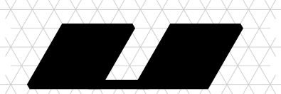
Figure 2: An example of an object with a tunnel of width 1.

A configuration $C$ is legal if and only if all particles are contracted and

$$\min_{v\in V_{\text{eqt}}\setminus(V(P)\cup V(O))}d(v,V(O))\geq\max_{v\in V(P)}d(v,V(O))$$

i.e., the particles are as close to the object as possible, which means that they coat $O$ as evenly as possible.

An algorithm solves the universal coating problem if, starting from any valid configuration, it reaches a stable legal configuration $C$ in a finite number of rounds. A configuration $C$ is said to be stable if no particle in $C$ ever performs a state change or movement.

1.3 Our Contributions

Our main contribution in this paper is a worst-case work-optimal algorithm for the universal coating problem on self-organizing particle systems. Our Universal Coating Algorithm seamlessly adapts to any valid object $O$, uniformly coating the object by forming multiple coating layers if necessary. As stated in Section 1.1, our particles are anonymous, do not have any global information (including on the number of particles $n$), have constant-size memory, and utilize only local interactions.

Our algorithm builds upon many primitives, some of which may be of interest on their own: The spanning forest primitive organizes the particles into a spanning forest which is used to guide the movement of particles while preserving connectivity in the system; the complaint-based coating primitive allows the first layer to form, only expanding the coating of the first layer as long as there is still room and there are particles still not touching the object; the general layering primitive allows the layer $\ell$ to form only after layer $\ell-1$ has been completed, for $\ell\geq 2$; and a node-based leader election primitive elects a position (in $G_{\text{eqt}}$) to house a leader particle, which is used to jumpstart the general layering process. One of the main contributions of our work is to show how these primitives can be integrated in a seamless way, with no underlying synchronization mechanisms.

1.4 Related work

Many approaches have already been proposed that can potentially be used for smart coating. One can distinguish between active and passive systems. In passive systems the particles either do not have any intelligence at all (but just move and bond based on their structural properties or due to chemical interactions with the environment), or they have limited computational capabilities but cannot control their movements. Examples of research on passive systems are DNA self-assembly systems (see, e.g., the surveys in [3, 4, 5]), population protocols [6], and slime molds [7, 8]. We will not describe these models in detail since we are focusing on active systems. In active systems, computational particles can control the way they act and move in order to solve a specific task. Robotic swarms, and modular robotic systems are some examples of active programmable matter systems.

Especially in the area of swarm robotics the problem of coating objects has been studied extensively. In swarm robotics, it is usually assumed that there is a collection of autonomous robots that have limited sensing, often including vision, and communication ranges, and that can freely move in a given area. However, coating of objects is commonly not studied as a stand-alone problem, but is part of collective transport (e.g., [9]) or collective perception (see respective section of [10, 11] for a summary of results). In collective transport a group of robots has to cooperate in order to transport an object. In general, the object is heavy and cannot be moved by a single robot, making cooperation necessary. In collective perception, a group of robots with a local perception each (i.e., only a local knowledge of the environment), aims at joining multiple instances of individual perceptions to one big global picture (e.g. to collectively construct a sort of map). Some research focuses on coating objects as an independent task under the name of target surrounding or boundary coverage. The techniques used in this context include stochastic robot behaviors [12, 13], rule-based control mechanisms [14] and potential field-based approaches [15]. Surveys of recent results in swarm robotics can be found in [16, 17, 10, 11]; other samples of representative work can be found in e.g., [18, 19, 20, 21, 22]. While the analytic techniques developed in the area of swarm robotics and natural swarms are of some relevance for this work, the individual units in those systems have more powerful communication and processing capabilities than the systems we consider, and they can move freely.

In a recent paper [23], Michail and Spirakis propose a model for network construction that is inspired by population protocols [6]. The population protocol model relates to self-organizing particles systems, but is also intrinsically different: agents (which would correspond to our particles) freely move in space and can establish connections to any other agent in the system at any point in time, following the respective probabilistic distribution. In the paper the authors focus on network construction for specific topologies (e.g., spanning line, spanning star, etc.). However, in principle, it would be possible to adapt their approach also for studying coating problems under the population protocol model.

1.5 Structure of the paper

Section 2 describes our Universal Coating algorithm. Formal correctness and worst-case work analyses of the algorithm follow in Section 3. We address some applications of our universal coating algorithm in Section 4, and present our concluding remarks in Section 5.

2 Universal Coating Algorithm

In this section we present our Universal Coating algorithm: In Section 2.1, we introduce some preliminary notions; Section 2.2 introduces the algorithmic primitives used for the coating algorithm; and lastly Section 2.3 focuses on the leader election process that is needed in certain instances of the problem.

2.1 Preliminaries

We define the set of states that a particle can be in as idle, follower, root, and retired. In addition to its state, a particle may maintain a constant number of flags (constant size pieces of information to be read by neighboring particles). While particles are anonymous, when a particle $p$ sets a flag of type $x$ in its shared memory, we will denote it by $p.x$ (e.g., $p.parent$, $p.dir$, etc.), so that ownership of the respective flag becomes clear. In our proposed algorithm, we assume that every time a particle contracts, it contracts out of its tail. Therefore, a node occupied by the head of a particle $p$ still is occupied by $p$ after a contraction.

We define a layer as the set of nodes $v$ in $G_{\text{eqt}}$ that are equidistant to the object $O$. More specifically a node $v$ is in layer $\ell$ if $d(v,V(O))=\ell$; in particular the surface coating layer defined earlier corresponds to layer 1. Any root or retired particle $p$ stores a flag $p.layer$ indicating the layer number of the node occupied by the head of $p$. We say a layer is filled or complete if all nodes in that layer are occupied with retired particles. In order to respect the particles’ constant-size memory constraints, we take all layer numbers modulo $4$. However, for ease of presentation, we will omit the modulo 4 computations in the text, except for in the pseudocode description of the algorithms.

Each root particle $p$ has a flag storing a port label $p.down$ pointing to an occupied node adjacent to its head in layer $p.layer-1$ or in the object if $p-layer=1$. Moreover, $p$ has two additional flags, $p.CW$ and $p.CCW$, which are also port labels. Intuitively, if $p$ continuously moves by expanding in direction $p.CW$ (resp., $p.CCW$) and then contracting, it moves along a clockwise (resp. counter-clockwise) path around the connected structure consisting of the object and retired particles. Formally, $p.CW$ is the label of the first port to a node $v$ in counter-clockwise (CCW) order from $p.down$ such that either $v$ is occupied by a particle $q$ with $q.layer=p.layer$, or $v$ is unoccupied (in the latter, $v$ may be a node on layer $p.layer$ or $p.layer-1$). We define $p.CCW$ analogously, following a clockwise (CW) order from $p.down$. Figure 3 illustrates the different layers around an object, and also CW and CCW traversals of those.

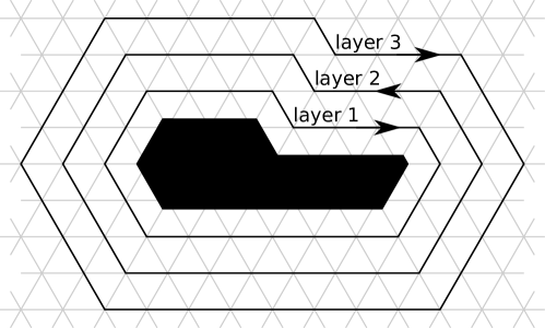
Figure 3: We illustrate the first three coating layers with respect to the given object (represented by the nodes in $G_{\text{eqt}}$ shaded in black); we also illustrate the direction in which these layers will be filled by our algorithm — CW for odd layers, and CCW for even layers — as determined in Section 2.2.

2.2 Coating Primitives

Our algorithm can be decomposed into a set of primitives, which are all concurrently executed by the particles, as we briefly described in Section 1.3. Namely the algorithm relies on the following key primitives: the spanning forest primitive, the complaint-based coating primitive used to establish the first layer of coating, the general layering primitive, and a node-based (rather than particle-based) leader election primitive that works even as particles move, and that is used to jumpstart the general layering primitive. One of the main contributions of our work is to show how these primitives can be put to work together in a seamless way and with no underlying synchronization mechanisms.

The spanning forest primitive (Algorithm 1) organizes the particles in a spanning forest, in which the roots of the trees will be in state root and will determine the direction of movement which is specified by a port label $p.dir$; the remaining non-retired particles follow the root particles using handovers. The main benefit of organizing the particles in a spanning forest connected to the surface is that it provides a relatively easy mechanism for particles to move, following the tree paths, while maintaining connectivity in the system (see [1, 25] for more details). All particles are initially idle. A particle $p$ becomes a follower when it sets a flag $p.parent$ corresponding to the port leading to its parent in the spanning forest (any adjacent particle $q$ to $p$ can then easily check if $q$ is a child of $p$). As the root particles find final positions according to the partial coating of the object, they stop moving and become retired. Namely, a root particle $p$ becomes retired when it encounters another retired particle across the direction $p.dir$.

A particle $p$ a acts depending on its state as described below:
idle: If $p$ is connected to the object $O$, it becomes a root particle, makes the current node it occupies a leader candidate position, and starts running the leader election algorithm described in Section 2.3. If $p$ is connected to a retired particle, $p$ also becomes a root particle. If an adjacent particle $p^{\prime}$ is a root or a follower, $p$ sets the flag $p.parent$ to the label of the port to $p^{\prime}$, puts a complaint flag in its local memory, and becomes a follower. If none of the above applies, $p$ remains idle. follower: If $p$ is contracted and connected to a retired particle or to $O$, then $p$ becomes a root particle. Otherwise, if $p$ is expanded, it considers the following two cases: $(i)$ if $p$ has a contracted child particle $q$, then $p$ initiates Handover$(p)$; $(ii)$ if $p$ has no children and no idle neighbor, then $p$ contracts. Finally, if $p$ is contracted, it runs the function ForwardComplaint$(p,p.parent)$ described in Algorithm 3. root: If particle $p$ is on the surface coating layer, $p$ participates in the leader election process described in Section 2.3. If $p$ is contracted, it first executes MarkerRetiredConditions$(p)$ (Algorithm 6), and becomes retired, and possibly also a marker, accordingly; if $p$ does not become retired, it calls LayerExtension $(p)$ (Algorithm 4). If $p$ is expanded, it considers the following two cases: $(i)$ if $p$ has a contracted child, then $p$ initiates Handover$(p)$; $(ii)$ if $p$ has no children and no idle neighbor, then $p$ contracts. Finally, if $p$ is contracted, it runs ForwardComplaint$(p,p.dir)$ (Algorithm 3). retired: $p$ clears a potential complaint flag from its memory and performs no further action.

Algorithm 1 Spanning Forest Primitive

Recall that $B$ denotes the number of nodes on the surface coating layer (layer 1). We need to ensure that once $\min\{n,B\}$ particles are on layer $1$, they stop moving and the coating is complete, independent of how $B$ compares to $n$ (i.e., whether $n\leq B$ or not); in addition, we would like to efficiently coat one more surface scenario, namely that of coating just a bounded segment of the surface, as we explain in Section 4. In order to be able to seamlessly adapt to all possible coating configurations, we use our novel complaint-based coating primitive for the first layer, which basically translates into having the root particles (touching the object) open up one more position on layer $1$ only if there exists a follower particle that remains in the system. This is accomplished by having each particle that becomes a follower generate a complaint flag, which will be forwarded by particles in a pipeline fashion from children to parents through the spanning forest and then from a root $q$ to another root at $q.dir$, until it arrives at a root particle $p$ with an unoccupied neighboring node at $p.dir$ (we call such a particle $p$ a super-root). Upon receiving a complaint flag, a super-root $p$ consumes the flag and expands into the unoccupied node at $p.dir$. The expansion will eventually be followed by a contraction of $p$, which will induce a series of expansions and contractions of the particles on the path from $p$ to a follower particle $z$, eventually freeing a position on the surface coating layer to be taken by $z$. In order to ensure that the consumption of a complaint flag will indeed result in one more follower touching the object, one must give higher priority to a follower child particle in a handover operation, as we do in Algorithm 2. The complaint-based coating phase of the algorithm will terminate either once all complaint flags are consumed or when layer $1$ is filled with contracted particles. In either case, the particles on layer $1$ will move no further. Figure 4 illustrates the complaint-based coating primitive.

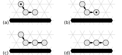
Figure 4: Complaint-based coating primitive: Particles are shown as grey circles. In (a), a follower particle generates a complaint flag (depicted as a black dot within the particle) that is then forwarded to a super-root (b) causing the super-root to expand into an unoccupied node (c). After a series of handovers, the follower particle that generated the complaint flag can move to a position on the surface (d).

1:if $p.layer=1$ and $p$ has a follower child $q$ then

2:     if $q$ is contracted then

3:         $p$ initiates a handover with particle $q$      

4:else

5:     if $p$ has any contracted (follower or root) child $q$ then

6:         $p$ initiates a handover with particle $q$      

Algorithm 2 Handover $(p)$

1:if $p$ holds a complaint flag and $p$’s parent does not hold a complaint flag then

2:     $p$ forwards the complaint flag to the particle given by $p.parent$

Algorithm 3 ForwardComplaint$(p,i)$

Once layer $1$ is complete and if there are still follower particles in the system, the general layering primitive steps in, which will build further coating layers. We accomplish this by electing a leader marker particle on layer $1$ (via the leader election primitive proposed in Section 2.3). This leader marker particle will be used to determine a “beginning” (and an “end”) for layer $1$ and allow the particles on that layer to start retiring according to the retired condition given in Algorithm 6 (the leader marker particle will be the first retired particle in the system). Once a layer $\ell$ becomes completely filled with retired (contracted) particles, a new marker particle will emerge on layer $\ell+1$, and start the process of building this layer (i.e., start the process of retiring particles on that layer) according to Algorithm 6. A marker particle on layer $\ell+1$ only emerges if a root particle $p$ connects to the marker particle $q$ on layer $\ell$ via its marker port and if $q$ verified locally that layer $\ell$ is completely filled (by checking whether $q.CW$ and $q.CCW$ are both retired).

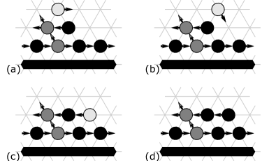
Figure 5: General layering primitive: Retired particles are shown as black circles, other than (retired) marker particles which are shown in dark grey (the dark grey arrows represent the marker edges); a root particle is depicted in light grey. Black arrows show the current direction of movement (given by the dir flag) for each particle (which becomes irrelevant once a particle retires). (a) The root particle $p$ is located on layer $\ell=3$; (b) particle $p$ moves in $CW$ direction over retired particles on layer $\ell-1$; (c) after a series of expansions and contractions following $p.dir$, $p$ arrives at an unoccupied neighboring node on layer $\ell-1$; (d) since $p.dir$ leads to a retired particle, $p$ retires too.

With the help of the marker particles — which can only be established after layer $1$ was completely filled (and hence, we must have $B\leq n$) — we can replace the complaint-based coating algorithm of layer $1$ with a simpler coating algorithm for the higher layers, where each root particle $p$ just moves in $CW$ or $CCW$ direction (depending on its layer number) until $p$ encounters a retired particle on the respective layer and retires itself. More precisely, each contracted root particle $p$ on layer $\ell$ tries to extend this layer by expanding into an unoccupied position on layer $\ell$, or by moving into an unoccupied position in layer $\ell-1$ (when $p.layer$ will change to $\ell-1$ accordingly), following the direction of movement given by $p.dir$. Figure 5 illustrates this process. The direction $p.dir$ is set to $p.CW$ (resp., $p.CCW$) when $p.layer$ is odd (resp., even), as illustrated in Figure 3. Alternating between $CCW$ and $CW$ movements for the particles in consecutive layers ensures that a layer $\ell$ is completely filled with retired particles before particles start retiring in layer $\ell+1$, which is crucial for the correctness of our layering algorithm.

1:Calculating $p.layer$, $p.down$ and $p.dir$

2:The layer number of any node occupied by the object is equal to 0.

3:Let $q$ be any neighbor of $p$ with smallest layer number (modulo $4$).

4:$p.down\;\leftarrow\;\mbox{$p$'s label for port leading to }q$

5:$p.layer=(q.layer+1)\mod\>4$

6:clockwise $(p,p.down)$ $\triangleright$ Computes CW & CCW directions

7:if $p.layer$ is odd then

8:     $p.dir\;\leftarrow\;p.CW$

9:else

10:     $p.dir\;\leftarrow\;p.CCW$

11:

12:Extending layer $p.layer$

13:if  the position at $p.dir$ is unoccupied, and either $p$ is not on the first layer, or $p$ holds a complaint flag then

14:     $p$ expands in direction $p.dir$

15:     $p$ consumes its complaint flag, if it holds one

Algorithm 4 LayerExtension $(p)$

1:$j\;\leftarrow\;i$, $k\;\leftarrow\;i$

2:while edge $j$ is connected to the object or to a retired particle with layer number $p.layer-1$ do

3:     $j\;\leftarrow\;(j-1)\mod 6$

4:$p.CW\;\leftarrow\;j$

5:while edge $k$ is connected to the object or to a retired particle with layer number $p.layer-1$ do

6:     $k\;\leftarrow\;(k+1)\mod 6$

7:$p.CCW\;\leftarrow\;k$

Algorithm 5 Clockwise $(p,i)$

1:First marker condition:

2:if $p$ is leader particle  then

3:     $p$ becomes a retired particle

4:     $p$ sets the flag $p.marker$ to be the label of a port leading to a node guaranteed not to be on layer $p.layer$ — e.g., by taking the average direction of $p$’s two neighbors in layer $1$ (by now complete)

5:

6:Extending Layer Markers:

7:if $p$ is connected to a marker $q$ and the port $q.marker$ points towards $p$ then

8:     if both $q.CW$ and $q.CCW$ are retired then

9:         $p$ becomes a retired particle

10:         $p$ sets the flag $p.marker$ to the label of the port opposite of the port connecting $p$ to $q$      

11:

12:Retired Condition:

13:if edge $p.dir$ is occupied by a retired particle then

14:     $p$ becomes retired

Algorithm 6 MarkerRetiredConditions$(p)$

2.3 Leader Election Primitive

In this section, we describe the process used for electing a leader among the particles that touch the object. Note that only particles in layer $1$ will ever participate in the leader election process. A leader will only emerge if $B\leq n$; otherwise the process will stop at some point without a leader being elected. As discussed earlier, a leader is elected on layer $1$ to provide a “checkpoint” (a marker particle) that the particles can use in order to determine whether the layer has been completely filled (and a leader is only elected after this happens).

The leader election algorithm we use in this paper is a slightly modified version of the leader election algorithm presented in [1] that can tolerate particles moving around on the surface layer while the leader election process is progressing (in [1], leader election runs on a system of static particles). Hence, for the purpose of universal coating, we will abstract the leader election algorithm to conceptually run on the nodes in layer $1$, and not on the particular particles that may occupy these nodes at different points in time. The particles on layer 1 will simply provide the means for running the leader election process on the respective positions, storing and transferring all the flags (which can be used to implement the tokens described in [1]) that are needed for the leader competition and verification. An expanded particle $p$ on layer 1, whose tail occupies node $v$ in layer $1$, that is about to perform a handover with contracted particle $q$ will pass all the information associated with $v$ to $q$ using the particles’ local shared memories. If a particle $p$ occupying position $v$ would like to forward some leader election information to a node $w$ adjacent to $v$ that is currently unoccupied, it will wait until either $p$ itself expands into $w$, or another particle occupies node $w$. It is important to note that according to the complaint-based coating algorithm that we run on layer $1$, if a node $v$ in layer $1$ is occupied at some time $t$, then $v$ will never be left unoccupied after time $t$.

Here we outline the differences between the leader election process used in this paper and that of [1]:

• Only the nodes on layer $1$ that initially hold particles start as leader node candidates. Other nodes in layer $1$ will take part in the leader node election process by forwarding any tokens between two consecutive leader node candidates, as determined for the leader election process for a set of static particles forming a cycle in [1]. Note that layer 1 is a cycle on $G_{\text{eqt}}$.

• The leader election process will determine which leader node candidate in layer $1$ will emerge as the unique leader node. The leader particle is then chosen as described below.

• If particle $p$ is expanded, it will hold the flags and any other information necessary for the leader election process corresponding to each node $p$ occupies (head and tail nodes) independently. In other words, an expanded particle emulates the leader election process for two nodes on the surface layer.

• A particle $p$ occupying node $v$ forwards a flag $\tau$ to the node $w$ in CW (or CCW) direction along the surface layer only if node $w$ is occupied by a particle $q$ (note that $q$ may be equal to $p$, if $p$ is expanded) and $q$ has enough space in its (constant-size) memory associated with node $w$; otherwise $p$ continues to hold the flag $\tau$ in its shared memory associated with node $v$.

• If $p$ is expanded along an edge $(v,w)$ and wants to contract into node $w$, there must exist a particle $q$ expanding into $v$ (due to the complaint-based mechanism), and hence $p$ will transfer all of its flags currently associated with node $v$ to particle $q$.

After the solitude verification phase in the leader election algorithm of [1] is complete, there will be just one leader node $v$ left in the system. Once $v$ is elected a leader node, a contracted particle $p$ occupying this position will check if layer $1$ is completely filled with contracted particles. To do so, when a contracted particle $p$ occupies node $v$ it will generate a single CHK flag which it will forward to its CCW neighbor $q$ only if $q$ is contracted. Any particle $q$ receiving a CHK flag will also only forward the flag to its CCW neighbor $z$ if and only if $z$ is contracted. If the CHK flag at a particle $q$ ever encounters an expanded CCW neighbor, the flag is held back until the neighbor contracts. Additionally, the particle at position $v$ sends out a CLR flag to its CW neighbor as soon as it expands. This flag is always forwarded in CW direction. If a CLR and a CHK flag meet at some particle, the flags cancel each other out. If at some point in time, a particle $p$ at node $v$ receives a CHK flag from its CW neighbor in layer $1$, it implies that layer $1$ must be completely filled with contracted particles (and the complaint-based algorithm for layer $1$ has converged), and at that time this contracted particle $p$ elects itself the leader particle, setting the flag $p.leader$. Note that the leader election process itself does not incur any additional particle expansions or contractions on layer 1, only the complaint-based algorithm does.

3 Analysis

In this section we show that our algorithm eventually solves the coating problem, and we bound its worst-case work.

We say a particle $p^{\prime}$ is the parent of particle $p$ if $p^{\prime}$ occupies the node in direction $p.parent$. Let an active particle be a particle in either follower or root state. We call an active particle a boundary particle if it has the object or at least one retired particle in its neighborhood, otherwise it is a non-boundary particle. A boundary particle is either a root or a follower, whereas non-boundary particles are always followers. Note that throughout the analysis we ignore the modulo computation of layers done by the particles, i.e., layer $1$ is the unique layer of nodes with distance $1$ to the object.

Given a configuration $C$, we define a directed graph $A(C)$ over all nodes in $G_{\text{eqt}}$ occupied by active particles in $C$. For every expanded active particle in $C$, $A(C)$ contains a directed edge from the tail to the head node of $p$. For every non-boundary particle $p$, $A(C)$ has a directed edge from the head of $p$ to $p.parent$, if $p.parent$ is occupied by an active particle, and for every boundary particle $p$, $p$ has a directed edge from its head to the node in the direction of $p.dir$ as it would be calculated by Algorithm 4, if $p.dir$ is occupied by an active particle. The ancestors of a particle $p$ are all nodes reachable by a path from the head of $p$ in $A(C)$. For each particle $p$ we denote the ancestor that has no outgoing edge with $p.superRoot$, if it exists. Certainly, since every node has at most one outgoing edge in $A(C)$, the nodes of $A(C)$ can only form a collection of disjoint trees or a ring of trees. We define a ring of trees to be a connected graph consisting of a single directed cycle with trees rooted at it.

First, we prove several safety conditions, and then we prove various liveness conditions that together will allow us to prove that our algorithm solves the coating problem.

3.1 Safety

Suppose that we start with a valid instance $(P,O)$, i.e., all particles in $P$ are initially contracted and idle and $V(P)\cup V(O)$ forms a single connected component in $G_{\text{eqt}}$, among other properties. Then the following properties hold, leading to the fact that $V(P)\cup V(O)$ stays connected at any time.

Lemma 1.

At any time, the set of retired particles forms completely filled layers except for possibly the current topmost layer $\ell$, which is consecutively filled with retired particles in $CCW$ direction (resp. $CW$ direction) if $\ell$ is odd (resp. even).

Proof.

From our algorithm it follows that the first particle that retires is the leader particle, setting its marker flag in a direction not adjacent to a position in layer 1. The particles in layer 1 then retire starting from the leader in $CCW$ direction around the object. Once all particles in layer 1 are retired, the first particle to occupy the adjacent position to the leader via its marker flag direction will retire and become a marker particle on layer 2, extending its marker flag in the same direction as the flag set by the marker (leader) on layer 1. Starting from the marker particle in layer 2, other contracted boundary particles can retire in $CW$ direction along layer 2. Once all particles in layer 2 are retired, the next layer will start forming. This process continues inductively, proving the lemma. ∎

The next lemma characterizes the structure of $A(C)$.

Lemma 2.

At any time, $A(C)$ is a forest or a ring of trees. Any node that is a super-root (i.e., the root of a tree in $A(C)$) or part of the cycle in the ring of trees is connected to the object or to a retired particle.

Proof.

An active particle can either be a follower or a root. First, we show the following claim.

Claim 1.

At any time, $A(C)$ restricted to non-boundary particles forms a forest.

Proof.

Let $A^{\prime}(C)$ be the induced subgraph of $A(C)$ by the non-boundary particles only. Certainly, at the very beginning, when all particles are still idle, the claim is true. So suppose that the claim holds up to time $t$. We will show that it then also holds at time $t+1$. Suppose that at time $t+1$ an idle particle $p$ becomes active. If it is a non-boundary particle (i.e., a follower), it sets $p.parent$ to a node occupied by a particle $q$ that is already active, so it extends the tree of $q$ by a new leaf, thereby maintaining a tree. Edges can only change if followers move. However, followers only move by a handover or a contraction, thus a handover can only cause a follower and its incoming edges to disappear from $A^{\prime}(C)$ (if that follower becomes a boundary particle), and an isolated contraction, can only cause a leaf and its outgoing edge to disappear from $A^{\prime}(C)$, so a tree is maintained in $A^{\prime}(C)$ in each of these cases. ∎

Next we consider $A(C)$ restricted to boundary particles.

Claim 2.

At any time, $A(C)$ restricted to boundary particles forms a forest or a ring.

Proof.

The boundary particles always occupy the nodes adjacent to retired particles or the object. Therefore, due to Lemma 1, the boundary particles either all lie in a single layer or in two consecutive layers. Since the layer numbers uniquely specify the movement direction of the particles, connected boundary particles within a layer are all connected in the same orientation. Therefore, if these particles all lie in a single layer, they can only form a directed list or directed cycle in $A(C)$, proving the claim. If they lie in two consecutive layers, say, $\ell$ and $\ell-1$, then $\ell-1$ must contain at least one retired particle, so the nodes occupied by the boundary particles in layer $\ell-1$ can only form a directed list. If there are at least two boundary particles in layer $\ell-1$, this must also be true for the nodes occupied by the boundary particles in layer $\ell$ because according to Lemma 1 there must be at least two consecutive nodes in layer $\ell-1$ not occupied by retired particles. Moreover, it follows from the algorithm that $p.dir$ of a boundary particle can only point to the same or the next lower layer of $p$, implying that in this case $A(C)$ restricted to the nodes occupied by all boundary particles forms a forest. ∎

Since a boundary particle $p$ never connects to a non-boundary particle the way $p.dir$ is defined, and a follower without an outgoing edge in $A(C)$ restricted to the non-boundary particles must have an outgoing edge to a boundary particle (otherwise it is a boundary particle itself), $A(C)$ is a forest or a ring of trees. The second statement of the lemma follows from the fact that every boundary particle must be connected to the object or a retired particle. ∎

Finally, we investigate the structure formed by the idle particles.

Lemma 3.

At any time, every connected component of idle particles is connected to at least one non-idle particle or the object.

Proof.

Initially, the lemma holds by the definition of a valid instance. Suppose that the lemma holds at time $t$ and consider a connected component of idle particles. If one of the idle particles in the component is activated, it may either stay idle or change to an active particle, but in both cases the lemma holds at time $t+1$. If a retired particle that is connected to the component is activated, it does not move. If a follower or root particle that is connected to the component is activated, that particle cannot contract outside of a handover with another follower or root particle, which implies that no node occupied by it is given up by the active particles. So in any of these cases, the connected component of idle particle remains connected to a non-idle particle. Therefore, the lemma holds at time $t+1$. ∎

The following corollary is consequence of the previous three lemmas.

Corollary 1.

At any time, $V(P)\cup V(O)$ forms a single connected component.

Lemma 4.

At any time before the first particle retires, in every connected component $G$ of $A(C)$, the number of expanded boundary particles in $G$ plus the number of complaint flags in $G$ is equal to the number of non-boundary particles in $G$.

Proof.

Initially, the lemma holds trivially. Suppose the lemma holds at time $t$ and consider the next activation of a particle. We only discuss relevant cases. If an idle particle becomes a non-boundary particle (i.e., it is not connected to the object but joins a connected component), it also generates a complaint flag. So both the number of non-boundary particles and the number of complaint flags increases by one for the component the particle joins. If a non-boundary particle expands as part of a handover with a boundary particle, both the number of expanded boundary particles and the number of non-boundary particles decrease by one for the component. If a boundary particle expands as part of a handover, that handover must be with another boundary particle, so the number of expanded boundary particles remains unchanged for that component. Since by our assumption there is no retired particle, all boundary particles are in layer 1. Hence, for a boundary particle to expand outside of a handover, it has to consume a complaint flag. This increases the number of expanded boundary particles by one and decreases the number of complaint flags by one. Finally, an expansion of a boundary particle outside of a handover can connect two components of $A(C)$. Since the equation given in the lemma holds for each of these components individually, it also holds for the newly built component. ∎

3.2 Liveness

We say that the particle system makes progress if (i) an idle particle becomes active, or (ii) a movement (i.e., an expansion, handover, or contraction) is executed, or (iii) an active particle retires. In the following, we always assume that we have a fair activation sequence for the particles.

Before we show under which circumstances our particle system eventually makes progress, we first establish some lemmas on how particles behave during the execution of our algorithm.

Lemma 5.

Eventually, every idle particle becomes active.

Proof.

As long as an idle particle exists, there is always an idle particle $p$ that is connected to a non-idle particle or the object according to Lemma 3. The next time $p$ is activated $p$ becomes active according to Algorithm 1. Therefore, eventually all particles become active. ∎

The following statement shows that even though super-roots can be followers, they will become a boundary particle the next time they are activated.

Lemma 6.

In every tree of $A(C)$, every boundary particle in the follower state enters a root state the next time it is activated. In particular, every super-root in $A(C)$ will enter the root state the next time it is activated.

Proof.

Let $p$ be a follower boundary particle. By definition $p$ must have a retired particle or the object in its neighborhood. Therefore, $p$ immediately becomes a root particle once it is activated according to Algorithm 1. ∎

Furthermore, the following lemma provides a relation between the movement of super-roots and the availability of complaint flags.

Lemma 7.

For every tree of $A(C)$ with a contracted super-root $p$ and at least one complaint flag, $p$ will eventually retire or expand to $p.dir$, thereby consuming a complaint flag, and after the expansion $p$ may cease to be a super-root.

Proof.

If $p$ is not a root, it becomes one the next time it is activated according to Lemma 6. Therefore, assume $p$ is a root. If there is a retired particle in $p.dir$, $p$ retires and ceases to be a super-root. If the node in $p.dir$ is unoccupied, $p$ can potentially expand. According to Algorithm 3, complaint flags are forwarded along the tree of $p$ towards $p$. Once the flag reaches $p$, it will expand, thereby consuming the flag. If $p$ expands, it might have an active particle in its movement direction and thus ceases to be a super-root. ∎

Next, we prove the statement that expanded particles will not starve, i.e., they will eventually contract.

Lemma 8.

Eventually, every expanded particle contracts.

Proof.

Consider an expanded particle $p$ in a configuration $C$. By Lemma 5 we can assume w.l.o.g. that all particles in $C$ are active or retired. If there is no particle $q$ with either $q.parent=p$ or $p$ occupying the node in $q.dir$, then $p$ can contract once it is activated. If such a $q$ exists and it is contracted, $p$ contracts in a handover (see Algorithm 2). If $q$ exists and is expanded, we consider the tree of $A(C)$ that $p$ is part of. Consider a subpath in this tree that starts in $p$, i.e., $(v_{1},v_{2},\ldots,v_{k})$ such that $v_{1},v_{2}$ are occupied by $p$ and $v_{k}$ is a node that does not have an incoming edge in $A(C)$. Let $v_{i}$ be the first node of this path that is occupied by a contracted particle. If all particles are expanded, then clearly the last particle occupying $v_{k-1},v_{k}$ eventually contracts and we can set $v_{i}$ to $v_{k-1}$. Since $v_{i}$ is contracted it eventually performs a handover with the particle occupying $v_{i-2},v_{i-1}$. Now we can move backwards along $(v_{1},v_{2},\ldots,v_{i-1})$ and it is guaranteed that a contracted particle eventually performs a handover with the expanded particle occupying the two nodes before it on the path. So eventually $q$ is contracted, eventually performs a handover with $p$ and the statement holds. ∎

In the following two lemmas we will specifically consider the case that $B\leq n$, i.e., the particles can coat at least one layer around the object.

Lemma 9.

If $B\leq n$, layer $1$ is completely filled with contracted particles eventually.

Proof.

Consider a configuration $C$ such that layer $1$ is not completely filled by contracted particles. Note that in this case the leader election cannot have succeeded yet, which means that a leader cannot be elected, and therefore no particle can be retired in configuration $C$. So by Lemma 5 we can assume w.l.o.g. that all particles in configuration $C$ are active.

Since layer 1 is not completely filled by contracted particles, there is either at least one unoccupied node $v$ on layer $1$ or all nodes are occupied, but there is at least one expanded particle on layer $1$. We show that in both cases a follower will move to layer $1$, thereby filling up the layer until all particles are contracted. In the first case, let $p$ be the super-root of a tree in $A(C)$ that still has non-boundary particles, let $(p_{0}=p,p_{1},\ldots,p_{k})$ be the boundary particles of the tree such that $p_{i-1}$ occupies the node in $p_{i}.dir$ and let $q$ be the non-boundary particle in the tree that is adjacent to some $p_{j}in(p_{0},\ldots,p_{k})$ such that $j$ is minimal. If a particle $p_{i}$ in $(p_{0},\ldots,p_{j}=q.parent)$ is expanded, it eventually contracts (Lemma 8) by a handover with $p_{i+1}$, and by consecutive handovers all particles in $(p_{i+1},\ldots,p_{j})$ eventually expand and contract until the particle $p_{j}=q.parent$ expands. According to Algorithm 2, $p_{j}$ performs a handover with $q$. Therefore, the number of particles on layer $1$ has increased. If all particles in $(p_{0},\ldots,q.parent)$ are contracted, then by Lemma 4 a complaint flag still exists in the tree. Eventually, $p$ expands by Lemma 7. Consequently, we are back in the former case that a particle in $(p_{0},\ldots,q.parent)$ is expanded.

In the second case, let $p^{\prime}$ be an expanded boundary particle and let $q^{\prime}$ be the non-boundary particle with the shortest path in $A(C)$ to $p^{\prime}$. By a similar argument as for the first case, particles on layer $1$ perform handovers (starting with $p^{\prime}$) until eventually the node in $q^{\prime}.parent$ is occupied by a tail. Again, $q^{\prime}$ eventually performs a handover and the number of particles on layer $1$ has increased. ∎

As a direct consequence, we can show the following.

Lemma 10.

If $B\leq n$, a leader is elected in layer $1$ eventually.

Proof.

According to Lemma 9 layer $1$ is eventually filled with contracted particles. Leader Election successfully elects a leader node according to [1]. The contracted particle $p$ occupying the leader node forwards the CHK flag and eventually receives it back, since all particles are contracted. Therefore, $p$ becomes a leader. ∎

Now we are ready to prove the two major statements of this subsection that define two conditions for system progress.

Lemma 11.

If all particles are non-retired and there is either a complaint flag or an expanded particle, the system eventually makes progress.

Proof.

If there is an idle particle, progress is ensured by Lemma 5. If an active particle is expanded Lemma 8 guarantees progress. Finally, in the last case all particles are active, none of them is expanded and there is a complaint flag. If layer $1$ is completely filled, a leader is elected according to Lemma 10 and as a direct consequence the active particles on layer $1$ eventually retire, guaranteeing progress. If layer $1$ is not completely filled, there exists at least one tree of $A(C)$ with a contracted super-root $p$ that has an unoccupied node in $p.dir$ and at least one complaint flag. Therefore, progress is ensured by Lemma 7. ∎

Lemma 12.

If there is at least one retired particle and one active particle, the system eventually makes progress.

Proof.

Again, if there is an idle particle, progress is ensured by Lemma 5. Moreover, note that since there is at least one retired particle, we can conclude that leader election has been successful (since the first particle that retires is a leader particle) and therefore layer $1$ has to be completely filled with contracted particles. If there is still a non-retired particle on layer $1$, it eventually retires according to the Algorithm, guaranteeing progress.

So suppose that all particles in layer 1 are retired. We distinguish between the following cases: (i) there exists at least one super-root, (ii) no super-root exists, but there is an expanded particle, and (iii) no super-root exists and all particles are contracted. In case (i), Lemma 6 guarantees that a super-root will eventually enter root state, and therefore it will eventually either expand (if $p.dir$ is unoccupied) or retire (since $p.dir$ is occupied by a retired particle). In case (ii), the particle contracts according to Lemma 8. In case (iii) $A(C)$ forms a ring of trees, which can only happen if all boundary particles completely occupy a single layer, so there is an active particle that occupies the node adjacent to the marker edge. Since it is contracted by assumption, it retires upon activation. Therefore, in all three cases the system eventually makes progress. ∎

3.3 Termination

Finally, we show that the algorithm eventually terminates in a legal configuration, i.e., a configuration in which the coating problem is solved. For the termination we need the following two lemmas.

Lemma 13.

The number of times an idle particle is transformed into an active one and an active particle is transformed into a retired one is bounded by $\mathcal{O}(n)$.

Proof.

From our algorithm it immediately follows that every idle particle can only be transformed once into an active particle, and every active particle can only be transformed once into a retired particle. Moreover, a non-idle particle can never become idle again, and a retired particle can never become non-retired again, which proves the lemma. ∎

Lemma 14.

The overall number of expansions, handovers, and contractions is bounded by $\mathcal{O}(n^{2})$.

Proof.

We will need the following fact, which immediately follows from our algorithm.

Fact 1.

Only a super-root of $A(C)$ can expand to a non-occupied node, and every such expansion triggers a sequence of handovers, followed by a contraction, in which every particle participates at most twice.

Consider any particle $p$. Note that only an active particle performs a movement. Let $C$ be the first configuration in which $p$ becomes active. If it is a non-boundary particle (i.e., a follower), then consider the directed path in $A(C)$ from the head of $p$ to the super-root $r$ of its tree or the first particle $r$ belonging to the ring in the ring of trees. Such a path must exist due to Lemma 2. Let $P=(v_{0},v_{1},\ldots,v_{m})$ be a node sequence covered by this path where $v_{0}$ is the head of $p$ in $C$ and $v_{m}$ is the first node along that path with the object or a retired particle in its neighborhood. Note that by Lemma 2 such a node sequence is well-defined since $v_{m}$ must at latest be a node occupied by $r$. According to Algorithm 1, $p$ attempts to follow $P$ by sequentially expanding into the nodes $v_{0},v_{1},\ldots,v_{m}$. At latest, $p$ will become a boundary particle once it reaches $v_{m}$. Up to this point, $p$ has traveled along a path of length at most $2n$, and therefore, the number of movements $p$ executes as a follower is $\mathcal{O}(n)$.

Now suppose $p$ is a boundary particle. Let $C$ be the configuration in which $p$ becomes a boundary particle and let $\ell=p.layer$. Suppose that $\ell=1$. From our algorithm we know that at most $n$ complaint flags are generated by the particles, and therefore by Lemma 7, there are at most $n$ expansions in level 1 (the rest are handovers or contractions). Hence, it follows from Fact 1 that $p$ can only move $\mathcal{O}(n)$ times as a boundary particle.

Next consider the case that $\ell>1$. Here we will need the following well-known fact.

Fact 2.

Let $B_{i}$ be the length of layer $i$. For every $i$ and every valid instance $(P,O)$ allowing $O$ to be coated by $i$ layers it holds that $B_{i}=B_{0}+6i$.

If $\ell=2$, there must be a retired particle in layer 1, and since the leader is the first retired particle, Lemmas 9 and 10 imply that level $\ell-1$ is completely filled with contracted particles. So $p$ can only move along nodes of layer $\ell$. Since $B_{\ell-1}\leq n$, it follows from Fact 2 that $B_{\ell}\leq n+6$. As long as not all particles in level $\ell-1$ are retired, $p$ cannot move beyond the marker node in level $\ell$. So $p$ either becomes retired before reaching the marker node, or if it reaches the marker node, it has to wait there till all particles in level $\ell-1$ are retired, which causes the retirement of $p$. Therefore, $p$ moves along at most $n+6$ nodes. If $\ell>2$, we know from Lemma 1 that level $\ell-2$ is completely filled with contracted particles. Since $B_{\ell-2}\leq n$ and $B_{\ell}=B_{\ell-2}+12$, it follows that $B_{\ell}\leq n+12$. Hence, $p$ will move along at most $n+12$ nodes in level $\ell$ before becoming retired or moving to level $\ell-1$, and $p$ will move along at most $n+6$ further nodes in level $\ell-1$ before retiring.

Thus, in any case, $p$ performs at most $\mathcal{O}(n)$ movements as a boundary particle. Therefore, the number of movements any particle in the system performs is $\mathcal{O}(n)$, which concludes the lemma. ∎

Lemmas 13 and 14 imply that the system can only make progress $\mathcal{O}(n^{2})$ many times. Hence, eventually our system reaches a configuration in which it no longer makes progress, so the system terminates. It remains to show that when the algorithm terminates, it is in a legal configuration, i.e., the algorithm solves the coating problem.

Theorem 1.

Our coating algorithm terminates in a legal configuration.

Proof.

From the conditions of Lemmas 11 and 12 we know that the following facts must both be true when the algorithm terminates:

1. At least one particle is retired or there is neither a complaint flag nor an expanded particle in the system (Lemma 11).

2. Either all particles are retired or all particles are active (Lemma 12).

First suppose that all particle are retired. Then it follows from Lemma 1 that the configuration is legal. Next, suppose that all particles are active and neither a complaint flag nor an expanded particle is left in the system. Then Lemma 4 implies that there cannot be any non-boundary any more, so all active particles must be boundary particles. If there is at least one boundary particle in layer $\ell>1$, then there must be at least one retired particle, contradicting our assumption. So all boundary particles must be in layer 1, and since there are no more complaint flags and all boundary particles are contracted, also in this case our algorithm has reached a legal configuration, which proves our theorem. ∎

Recall that the work performed by an algorithm is defined as the number of movements (expansions, handovers, and contractions) of the particles till it terminates. Lemma 14 implies that the work performed by our algorithm is $\mathcal{O}(n^{2})$. Interestingly, this is also the best bound one can achieve in the worst-case for the coating problem.

Lemma 15.

The worst-case work required by any algorithm to solve the Universal Object Coating problem is $\Omega(n^{2})$.

Proof.

Consider the configuration depicted in Figure 6.

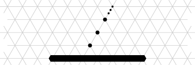
Figure 6: A worst-case configuration concerning work. The object is solid black and the non-object particles are black dots . Here, all $n$ particles lie on a straight line.

A particle with distance $i\geq 1$ to the object needs at least $2(i-1-\left\lceil\frac{i-1}{B}\right\rceil)$ movements to become contracted on its final layer. Therefore, any algorithm requires at least $2\sum_{i=1}^{n-1}(i-1-\left\lceil\frac{i-1}{B}\right\rceil)\geq\sum_{i=1}^{n-1}(i-1-(\frac{i}{B}))=\Omega(n^{2})$ work assuming $B\geq 2$. ∎

Hence, we get:

Theorem 2.

Our algorithm requires worst-case optimal work $\Theta(n^{2})$.

4 Applications

In this section, we present other coating scenarios and applications of our universal coating algorithm. Our algorithm can be easily extended to also handle the case when one would like to cover only a certain portion of the object surface. More concretely, assume that one would like to cover the portion of the object surface delimited by two endpoint nodes. Basically in that case, the algorithm can be modified slightly so that the particles that eventually reach one of the endpoints of the surface segment retire and become endpoint markers. The position of endpoint marker particles will be propagated to higher layers, as necessary, such that the delimited portion of the object is evenly coated.

Once the first layer is formed and a leader is elected (implying that $B\leq n$), one can trivially determine $(i)$ whether the number of particles in the system is greater than or equal to the size of the object boundary, or $(ii)$ whether the object $O$ is convex; one could also potentially address other applications that involve aggregating some (constant-size) collective data over the boundary of the object $O$. Once all particles in layer 1 retire, a leader will emerge and that leader can initiate the respective application. For the first application, all particles may initially assume that $B>n$. Once a leader is elected, it informs all other particles that $B\leq n$. For the convexity testing, the leader particle can generate a token that traverses the boundary in CW direction: If the token ever makes a left turn (i.e., it traverses two consecutive edges on the boundary at an outer angle of less than $180^{\circ}$), then the object is not convex; otherwise the object is convex.

5 Conclusion

This paper presented a universal coating algorithm for programmable matter using worst-case optimal work. It would be interesting to also bound the parallel runtime of our algorithm in terms of number of asynchronous rounds, and to investigate its competitiveness — i.e., how does its work or runtime compare to the best possible work or runtime for any given instance. Moreover, it would be interesting to implement the algorithm and evaluate its performance either via simulations or hopefully at some point even via experiments with real programmable matter.

References

- [1] Z. Derakhshandeh, R. Gmyr, T. Strothmann, R. A. Bazzi, A. W. Richa, C. Scheideler, Leader election and shape formation with self-organizing programmable matter, in: DNA Computing and Molecular Programming - 21st International Conference, DNA 21, Boston and Cambridge, MA, USA, August 17-21, 2015. Proceedings, 2015, pp. 117–132.
- [2] Z. Derakhshandeh, S. Dolev, R. Gmyr, A. W. Richa, C. Scheideler, T. Strothmann, Brief announcement: amoebot - a new model for programmable matter, in: 26th ACM Symposium on Parallelism in Algorithms and Architectures, SPAA ’14, Prague, Czech Republic - June 23 - 25, 2014, 2014, pp. 220–222.
- [3] D. Doty, Theory of algorithmic self-assembly, Communications of the ACM 55 (12) (2012) 78–88.
- [4] M. J. Patitz, An introduction to tile-based self-assembly and a survey of recent results, Natural Computing 13 (2) (2014) 195–224.
- [5] D. Woods, Intrinsic universality and the computational power of self-assembly, in: Proceedings Machines, Computations and Universality 2013, MCU 2013, Zürich, Switzerland, September 9-11, 2013., 2013, pp. 16–22. doi:10.4204/EPTCS.128.5.
- [6] D. Angluin, J. Aspnes, Z. Diamadi, M. J. Fischer, R. Peralta, Computation in networks of passively mobile finite-state sensors, Distributed Computing 18 (4) (2006) 235–253.
- [7] V. Bonifaci, K. Mehlhorn, G. Varma, Physarum can compute shortest paths, in: Proceedings of SODA ’12, 2012, pp. 233–240.
- [8] K. Li, K. Thomas, C. Torres, L. Rossi, C.-C. Shen, Slime mold inspired path formation protocol for wireless sensor networks, in: Proceedings of ANTS ’10, 2010, pp. 299–311.
- [9] S. Wilson, T. P. Pavlic, G. P. Kumar, A. Buffin, S. C. Pratt, S. Berman, Design of ant-inspired stochastic control policies for collective transport by robotic swarms, Swarm Intelligence 8 (4) (2014) 303–327.
- [10] M. Brambilla, E. Ferrante, M. Birattari, M. Dorigo, Swarm robotics: a review from the swarm engineering perspective, Swarm Intelligence 7 (1) (2013) 1–41. doi:10.1007/s11721-012-0075-2.
- [11] I. Navarro, F. Matía, An introduction to swarm robotics, in: ISRN Robotics, Hindawi Publishing Corporation, 2012, p. 10.
- [12] G. P. Kumar, S. Berman, Statistical analysis of stochastic multi-robot boundary coverage, in: 2014 IEEE International Conference on Robotics and Automation, ICRA 2014, Hong Kong, China, May 31 - June 7, 2014, 2014, pp. 74–81. doi:10.1109/ICRA.2014.6906592.
- [13] T. P. Pavlic, S. Wilson, G. P. Kumar, S. Berman, An enzyme-inspired approach to stochastic allocation of robotic swarms around boundaries, in: 16th International Symposium on Robotics Research (ISRR 2013), Singapore, Dec, 2013, pp. 16–19.
- [14] L. Blázovics, K. Csorba, B. Forstner, H. Charaf, Target tracking and surrounding with swarm robots, in: IEEE 19th International Conference and Workshops on Engineering of Computer-Based Systems, ECBS 2012, Novi Sad, Serbia, April 11-13, 2012, 2012, pp. 135–141. doi:10.1109/ECBS.2012.41.
- [15] L. Blázovics, T. Lukovszki, B. Forstner, Target surrounding solution for swarm robots, in: Information and Communication Technologies - 18th EUNICE/ IFIP WG 6.2, 6.6 International Conference, EUNICE 2012, Budapest, Hungary, August 29-31, 2012. Proceedings, 2012, pp. 251–262.
- [16] S. Kernbach (Ed.), Handbook of Collective Robotics – Fundamentals and Challanges, Pan Stanford Publishing, 2012.
- [17] J. McLurkin, Analysis and implementation of distributed algorithms for multi-robot systems, Ph.D. thesis, Massachusetts Institute of Technology (2008).
- [18] D. Arbuckle, A. Requicha, Self-assembly and self-repair of arbitrary shapes by a swarm of reactive robots: algorithms and simulations, Autonomous Robots 28 (2) (2010) 197–211.
- [19] R. Cohen, D. Peleg, Local spreading algorithms for autonomous robot systems, Theoretical Computer Science 399 (1-2) (2008) 71–82.
- [20] S. Das, P. Flocchini, N. Santoro, M. Yamashita, On the computational power of oblivious robots: forming a series of geometric patterns, in: Proceedings of the 29th Annual ACM Symposium on Principles of Distributed Computing, PODC 2010, Zurich, Switzerland, July 25-28, 2010, 2010, pp. 267–276.
- [21] X. Defago, S. Souissi, Non-uniform circle formation algorithm for oblivious mobile robots with convergence toward uniformity, Theoretical Computer Science 396 (1-3) (2008) 97–112.
- [22] T.-R. Hsiang, E. Arkin, M. Bender, S. Fekete, J. Mitchell, Algorithms for rapidly dispersing robot swarms in unknown environments, in: Proceedings of the 5th Workshop on Algorithmic Foundations of Robotics (WAFR), 2002, pp. 77–94.
- [23] O. Michail, P. G. Spirakis, Simple and efficient local codes for distributed stable network construction, in: ACM Symposium on Principles of Distributed Computing, PODC ’14, Paris, France, July 15-18, 2014, 2014, pp. 76–85.
- [24] http://sops.cs.upb.de.
- [25] Z. Derakhshandeh, R. Gmyr, A. W. Richa, C. Scheideler, T. Strothmann, An algorithmic framework for shape formation problems in self-organizing particle systems, in: To appear in 2nd ACM International Conference on Nanoscale Computing and Communication (ACM NANOCOM 2015), 2015.