Vlasov Simulations of Electron-Ion Collision Effects on Damping of Electron Plasma Waves

Abstract

Collisional effects can play an essential role in the dynamics of plasma waves by setting a minimum damping rate and by interfering with wave-particle resonances. Kinetic simulations of the effects of electron-ion pitch angle scattering on Electron Plasma Waves (EPWs) are presented here. In particular, the effects of such collisions on the frequency and damping of small-amplitude EPWs for a range of collision rates and wave phase velocities are computed and compared with theory. Both the Vlasov simulations and linear kinetic theory find the direct contribution of electron-ion collisions to wave damping is about a factor of two smaller than is obtained from linearized fluid theory. To our knowledge, this simple result has not been published before.

Simulations have been carried out using a grid-based (Vlasov) approach, based on a high-order conservative finite difference method for discretizing the Fokker-Planck equation describing the evolution of the electron distribution function. Details of the implementation of the collision operator within this framework are presented. Such a grid-based approach, which is not subject to numerical noise, is of particular interest for the accurate measurements of the wave damping rates.

I Introduction

Simulations of kinetic processes in plasmas make use of either Particle-in-Cell (PIC) methods or direct discretization of the Vlasov equation based on an Eulerian (or grid-based) representation. Computations carried out with the latter approach are also referred to as Vlasov simulations. In the context of PIC simulations of laser plasma interactions, methods for including collisional effects have been implemented and validated Takizuka and Abe (1977); Cohen et al. (2010); Dimits et al. (2013), and the effect of their inclusion has been shown in studies of stimulated Brillouin scattering with ion-ion collisions,Cohen et al. (2006) simulations of fast ignition with electron collisions,Kemp et al. (2010) and with electron-ion, electron-electron and ion-ion collisions in simulations of counter-streaming plasma flows.Ross et al. (2013) Recent developments have seen the application of multidimensional grid-based simulation,Banks et al. (2011a); Winjum et al. (2013); Berger et al. (2015) but collisions were not included in these studies.

When collisional effects are strong enough to enforce a nearly isotropic or Maxwell-Boltzmann distribution, methods such as ’Fokker-Planck’,Epperlein (1994); Brunner and Valeo (2002); Tzoufras et al. (2011) hydrodynamic descriptions,Braginskii (1965) or nonlocal hydrodynamic descriptions Albritton et al. (1986); Epperlein and Short (1991); Bychenkov et al. (1995); Brantov et al. (1996); Schurtz et al. (2000) may be applicable. Collisional effects may be important to consider in kinetic simulations as they can set a minimum damping rate for high phase velocity Electron Plasma (or Langmuir) Waves (EPWs) and ion acoustic waves in single-ion species Brantov et al. (2012); Epperlein et al. (1992) or multiple-ion species plasmas.Berger and Valeo (2005) In inertial fusion applications, collisional damping $\nu_{\rm coll}$ of EPWs is very weak, e.g., $\nu_{\rm coll}/\omega_{pe}\simeq\nu_{ei}^{\rm brag}/(2\omega_{pe})\sim 10^{-4}$ for a helium plasma at electron temperature $T_{e}=2.5~{}keV$ and electron density $N_{e}=ZN_{i}=9\cdot 10^{20}~{}cm^{-3}$ where $Z$ is the ion charge state and $N_{i}$ is the ion density. Here, $\omega_{pe}$ is the electron plasma frequency, and $\nu_{ei}^{\rm brag}$ is the electron-ion scattering rate as defined by Braginskii.Braginskii (1965) However, over the time scales that EPWs drive decay instabilities, i.e., time scales of the order of $\gtrsim 10^{3}\omega_{pe}^{-1}$ or larger, these loss rates may be significant Brunner et al. (2014); Berger et al. (2015). In addition, particles trapped by large amplitude waves can be scattered out of resonance by both pitch-angle scattering and thermalization in velocity space. Such processes have been estimated to limit the lifetime of BGK-type equilibria.Berger et al. (2013) In multiple spatial dimensions and for waves with a finite transverse width envelope, transverse convective losses must also be considered.Strozzi et al. (2012); Winjum et al. (2013) The most important collisional effects are often associated with pitch-angle scattering, whose primary effect is to change the direction of the particle’s velocity with negligible energy loss. Such redirected particles may carry energy away from a spatially localized wave. In this manuscript, we discuss the effects of pitch-angle collisions based on results from Vlasov-type simulations. In addition some details are provided concerning the implementation of collisions in the 4D = 2D+2V (two configuration space + two velocity space dimensions) Vlasov code LOKI,Banks and Hittinger (2010); Banks et al. (2011b) which uses fourth-order-accurate, conservative, finite-difference algorithms.

The effect of collisions on the Landau damping of EPWs has been the subject of a number of publications since the 1960s. A recent analytic treatment concerned the effect on the Landau resonance of weak electron-ion collisions in 3D velocity space Callen (2014) but earlier analytic studies were also done with 1D velocity diffusion operators.Su and Oberman (1968); Auerbach (1977); Zheng and Qin (2013) These studies did not consider the direct collisional damping of EPWs, analogous to inverse bremsstrahlung, and easily obtained from a fluid description by including drag in the electron momentum evolution equations. However, BrantovBrantov et al. (2004, 2012) considered the more general problem of EPW damping by using a Legendre expansion of the linearized Fokker-Planck equations including Landau collision operators. This work, similar to previous treatments of ion acoustic waves,Epperlein et al. (1992); Berger and Valeo (2005) found the combination of Landau and direct collisional damping appeared as separate summable effects.

In this work, we use the 2D+2V Vlasov code LOKI, including an electron-ion, pitch-angle collision operator, to compute the damping of an EPW initialized with a small-amplitude density perturbation. For weak electron-ion collisions, the perturbation decays exponentially in accord with the Landau damping rate for an EPW. For larger collision rates, we find an increase in the damping rate above the Landau rate because of collisional damping. Moreover, we find the damping directly attributable to collisions is about a factor of two smaller than we obtain from a linearized set of fluid equations with electron-ion momentum exchange. To our knowledge, this result has not been published before.

The remainder of this manuscript is organized as follows. The basic governing equations and discretization scheme used in the LOKI code are briefly reviewed in Section II. That section presents the collision operator considered in this work: A Lorentz pitch-angle scattering operator restricted to two-dimensional velocity space. Using the physically correct 3D collision operator is computationally prohibitive as it would require extending LOKI from a 2D to a 3D velocity grid. Detailed exposition of the numerical methods are given in Appendix A. The effects of collisions on EPW damping are discussed for a range of $k\lambda_{De}$ and $\nu_{ei,th}/\omega_{pe}$ (see Table 1) in Section III in the context of standing waves initiated with a density perturbation. Here, $k$ stands for the wave number and $\lambda_{De}$ for the electron Debye length. In Sec. III.1, a set of linearized kinetic equations in 3D spherical velocity coordinates ( Sec. III.1.1) and in 2D polar velocity coordinates (Sec. III.1.2) are presented for benchmarking LOKI simulation results. With use of this set of linearized equations, the differences between 2D and 3D collisional velocity diffusion on the EPW damping are examined in Sec III.2 and found to be modest. Also in this Section, the LOKI simulation results for the EPW frequency and damping rates are shown to be in excellent agreement with the 2D linearized set. The collisional damping of EPWs is obtained from a set of fluid equations for the density, flow velocity, and temperature in Sec.III.3 and shown to be about twice larger than obtained from the kinetic equations in the strongly collisional limit.

In addition to the EPW mode, additional weakly damped, zero-frequency ’entropy’ modes are observed in the solutions to linearized equations and in LOKI simulations. These modes are not the primary interest of the current work but their presence complicates the extraction of the EPW frequency and damping rates. As a result, Sec.III.5 discusses these modes in relation to mitigating their effect on computing EPW frequencies and damping rates.

The application of LOKI to a nonlinear problem is addressed in Sec. IV where the effect of pitch angle collisions on the trapping of electrons in a large-amplitude EPW is studied. Some concluding remarks are made in Section V. Finally the implementation of the pitch angle collision operator in the LOKI code is discussed in detail in Appendix A. It should be noted that although the results presented in this paper concern only electron-ion collisions, the collision algorithm in LOKI is implemented with the ability to study collisional ion dynamics as well, for an arbitrary number of ion species. In Appendix A, we also examine the effect that a cap on the pitch-angle collision rate (used in the numerical implementation of the collision operator) has on the results. The effect is insignificant if the cap is applied only at small velocity. In Appendix B, we find an approximate solution to the linear dispersion relation including pitch-angle collisions valid for $k\lambda_{ei}\ll 1$. We solve that dispersion relation in 2D and 3D and find a collisional EPW damping rate that agrees well with the Vlasov simulations.

II Vlasov Equation with Collisions in 2D+2V

We briefly describe the Vlasov-Poisson system of equations that LOKI solves for an unmagnetized plasma in two space and two velocity dimensions. The evolution with respect to time $t$ of the electron distribution function $f(x,y,v_{x},v_{y},t)$ is described by the Fokker-Planck equation, i.e. the Vlasov equation including collisional effects:

$${\frac{\partial f}{\partial t}+v_{x}\frac{\partial f}{\partial x}+v_{y}\frac{\partial f}{\partial y}}-\frac{e}{m_{e}}\left(E_{x}\frac{\partial f}{\partial v_{x}}+E_{y}\frac{\partial f}{\partial v_{y}}\right)=-C_{ei}f,$$ (1)

with $-e$ the elementary electric charge of the electron and $m_{e}$ its mass. The form of the electron-ion collision operator $C_{ei}f$ on the right-hand side of Eq. (1) will be discussed in detail in the next sub-section. The LOKI code Banks and Hittinger (2010); Banks et al. (2011b) discretizes the Vlasov equations in four dimensional phase space corresponding to the two-dimensional configuration space $(x,y)$ and the two-dimensional velocity space $(v_{x},v_{y})$. The electric field components are given through derivatives of the electric potential, $\phi(x,y,t)$:

$$E_{x}=-\frac{\partial\phi}{\partial x},\qquad E_{y}=-\frac{\partial\phi}{\partial y},$$

which is itself determined by Poisson’s equation,

$$\frac{\partial^{2}\phi}{\partial x^{2}}+\frac{\partial^{2}\phi}{\partial y^{2}}=4\pi e\left(\int_{-\infty}^{\infty}\int_{-\infty}^{\infty}f_{e}\,dv_{x}dv_{y}-\sum_{i}N_{i}Z_{i}\right),$$ (2)

where the sum is over all ion species of density $N_{i}$ and charge $Z_{i}e$ with overall charge neutrality assumed, $N_{e}=\sum_{i}N_{i}Z_{i}$, $N_{e}$ standing for the average electron density. Note that the Poisson equation (2) has been written in cgs units (this convention is kept throughout this paper) and that ions are considered as a fixed homogeneous, neutralizing background, which is a very good approximation for the simulations of EPWs that will be discussed.

We consider here the specific case of electron-ion pitch angle scattering, described by the Lorentz operator given by

$$C_{\rm ei}\,f = -\nu_{\rm ei,th}\,v_{\rm th\,e}^{3}\,\frac{\partial}{\partial\vec{v}}\cdot\mathbf{U}\cdot\frac{\partial f}{\partial\vec{v}},$$ (3)

$$\nu_{\rm ei,th} = 2\pi\frac{Ze^{4}N_{e}\log{\Lambda}}{m_{e}^{2}v_{\rm th\,e}^{3}},$$ (4)

where $\nu_{\rm ei,th}$ stands for the thermal electron-ion collision frequency , and the tensor $\mathbf{U}$ is defined by

$$\mathbf{U}(\vec{v})=\frac{1}{v^{3}}\left(v^{2}\mathbf{I}-\vec{v}:\vec{v}\right)=\frac{1}{v}\,\mathbf{P}_{\perp},$$ (5)

with $\mathbf{I}$ the identity tensor and $\mathbf{P}_{\perp}=\mathbf{I}-\vec{v}:\vec{v}/v^{2}$ the projection tensor on the plane perpendicular to the velocity $\vec{v}$.

In three-dimensional velocity space, spherical velocity variables $(v,\theta,\phi)$ are the natural coordinates for representing the rotationally invariant collision operator $C_{ei}$, with $v=|\vec{v}|$, $\theta$ the polar angle, and $\phi$ the azimuthal angle. The collision operator $C_{ei}$ can indeed be written:

$$C_{ei}=\nu_{\rm ei}(v)\,L^{2},$$ (6)

where $L^{2}$ is only dependent on the spherical-coordinate angles $(\theta,\phi)$:

$$L^{2} =-\left[\frac{1}{\sin\theta}\frac{\partial}{\partial\theta}\left(\sin\theta\frac{\partial}{\partial\theta}\right)+\frac{1}{\sin^{2}\theta}\frac{\partial^{2}}{\partial\phi^{2}}\right]$$

$$=-\left\{\frac{\partial}{\partial\xi}\left[(1-\xi^{2})\frac{\partial}{\partial\xi}\right]+\frac{1}{1-\xi^{2}}\frac{\partial^{2}}{\partial\phi^{2}}\right\},$$ (7)

with the pitch angle variable $\xi=\cos(\theta)$ and the velocity-dependent electron-ion collision frequency

$$\nu_{\rm ei}(v)=\nu_{\rm ei,th}\left(\frac{v_{\rm th\,e}}{v}\right)^{3}.$$ (8)

The eigenfunctions of the collision operator (6) are of the form:

$$f_{\lambda}(v,\theta)=\delta(v-v_{0})\,Y^{m}_{l}(\theta,\phi),$$ (9)

associated to the eigenvalues

$$\lambda=\nu_{\rm ei}(v_{0})\,l(l+1).$$ (10)

In Eq. (9), $\delta(v-v_{0})$ stands for the Dirac delta function centered at an arbitrary velocity amplitude $v_{0}\in\mathbb{R}_{+}$ and $Y^{m}_{l}(\theta,\phi)$ represents a spherical harmonic of degree $l\in\mathbb{N}$ and order $m\in\mathbb{Z}$, $m=-l,-l+1,\ldots,+l$. The spherical harmonics are given by

$$Y^{m}_{l}(\theta,\phi)=P^{m}_{l}(\cos\theta)\,e^{im\phi},$$

where the functions $P^{m}_{l}(\xi)$ are the associated Legendre polynomials of the first kind. In the LOKI model considered in this work, velocities are restricted to the two-dimensional space $(v_{x},v_{y})$, corresponding to the two Cartesian configuration space dimensions $(x,y)$. Reduction from the full three-dimensional velocity space to two-dimensional velocity space is necessary because discretization in six-dimensional [or even five-dimensional (2D+3V)] phase space remains computationally prohibitive. The natural coordinates for representing the collision operator (3) restricted to this two-dimensional velocity space are polar coordinates $(v,\theta)$, with $v=|\vec{v}|$ the velocity amplitude and the poloidal angle $\theta$ such that $\cos\theta=v_{x}/v$ and $\sin\theta=v_{y}/v$. In these coordinates the collision operator (3) takes the particularly simple form:

$$C_{ei}=-\nu_{\rm ei}(v)\frac{\partial^{2}}{\partial\theta^{2}},$$ (11)

with velocity dependent electron-ion collision frequency given by Eq. (8). The eigenfunctions of the collision operator (11) are of the form

$$f_{\lambda}(v,\theta)=\delta(v-v_{0})\,e^{im\theta},$$ (12)

associated to the eigenvalues

$$\lambda=\nu_{\rm ei}(v_{0})\,m^{2},$$ (13)

where $m\in\mathbb{Z}$ is an arbitrary integer and $\delta(v-v_{0})$ again stands for the Dirac delta function centered at an arbitrary velocity amplitude $v_{0}\in\mathbb{R}_{+}$.

In LOKI, velocity is however represented using the Cartesian coordinates $(v_{x},v_{y})$, a more natural representation for the collisionless advection dynamics defined by the left hand side of Eq. (1). The operator (11) must therefore also be expressed in the same coordinates $(v_{x},v_{y})$, which is a less natural choice for this collision term. Furthermore, in order to retain the strictly conservative formulation of LOKI, we express the two-dimensional pitch angle scattering operator in the conservative form:

$$C_{ei}f= \frac{\partial}{\partial\vec{v}}\cdot\vec{\Gamma}=\frac{\partial}{\partial v_{x}}\Gamma_{x}+\frac{\partial}{\partial v_{y}}\Gamma_{y}$$

$$= \,\left\{\frac{\partial}{\partial v_{x}}\left[\nu_{\rm ei}(v)v_{y}\left(v_{x}\frac{\partial f}{\partial v_{y}}-v_{y}\frac{\partial f}{\partial v_{x}}\right)\right]\right.$$

$$\hskip 22.76219pt\left.-\frac{\partial}{\partial v_{y}}\left[\nu_{\rm ei}(v)v_{x}\left(v_{x}\frac{\partial f}{\partial v_{y}}-v_{y}\frac{\partial f}{\partial v_{x}}\right)\right]\right\}.$$ (14)

Note that equation (14) can also be written in the following non-conservative form:

$$C_{ei}f=-\nu_{\rm ei}(v)\left(v_{x}\frac{\partial}{\partial v_{y}}-v_{y}\frac{\partial}{\partial v_{x}}\right)^{2}f,$$

obviously equivalent to (11) given that $\partial/\partial\theta=v_{x}\partial/\partial v_{y}-v_{y}\partial/\partial v_{x}$.

Discretization of the collision operator (14) using a higher order finite difference scheme is discussed in Appendix A. This appendix also explains how the velocity dependent collision frequency $\nu_{ei}(v)$ is slightly modified in LOKI for practical reasons. In particular, $\nu_{ei}(v)$ is capped at very low velocities: $\nu_{ei}(v)\equiv\nu_{ei}(\bar{v})=\nu_{ei,\max}$ for $v<\bar{v}\ll v_{\rm th\,e}$ [see Eq. (A7)]. Without this cap, the collision frequency diverges for velocities approaching zero, $\nu_{ei}(v)\sim v^{-3}\to\infty$ as $v\to 0$, and the time step required for the explicit time integration scheme implemented in LOKI would be impractically small. In Appendix A, results relevant to those discussed in the main part of this paper illustrate that a cap set as low as $\nu_{ei,\max}=10\,\nu_{ei,th}$, corresponding to $\bar{v}/v_{\rm th\,e}=10^{-1/3}\simeq 0.464$, has no discernable effect on the results for EPW damping. Furthermore, as $\nu_{ei}(v)\sim v^{-3}$, the collision rate naturally goes to zero as $v\to\infty$. However, for any finite maximum velocity of the grid, collisionality is non-zero and the collision operator therefore changes the nature of the equation from hyperbolic (i.e. purely advective) to parabolic, with undesirable consequences when implementing the boundary conditions. For that reason, the velocity dependent collision frequency $\nu_{ei}(v)$ is furthermore modified to smoothly go to zero for velocities $v_{c}<v<v_{\max}$, with $v_{c}$ short of the maximum value $v_{\max}$ of the grids along $v_{x}$ and $v_{y}$ [see as well Eq. (A7)]. Ensuring that $\nu_{ei}(v_{max})=0$ thus restores the hyperbolic boundary conditions, again with no effect on the results if $v_{max}$ is large enough. The results presented in Sec. III were carried out with $\nu_{ei,\max}=100\,\nu_{ei,th}$, which corresponds to $\bar{v}/v_{\rm th\,e}=100^{-1/3}\simeq 0.215$ and with $v_{max}/v_{\rm th\,e}=7$ for $k\lambda_{De}=0.3$ and $0.425$ but with $v_{max}/v_{\rm th\,e}=10$ for $k\lambda_{De}=0.2$.

III Collisional effects on Electron Plasma wave damping

When considering the Lorentz electron-ion pitch angle scattering collision operator restricted to two-dimensional velocity space instead of the full three-dimensional space, the question naturally arises how this approximation affects the collisional processes. To address this issue, we consider as a test problem the effect of varying collisionality on the damping, both Landau and collisional, of linear EPWs.

III.1 Linearized Kinetic Equations in Spherical and Polar Velocity Variables

In the following, we decompose the linearized Vlasov-Poisson system including the pitch angle scattering operator in three-dimensional velocity space, as described by Eqs. (6) and (7), using a Legendre polynomial representation (see e.g. Ref. Epperlein et al. (1992)). The Legendre polynomials (more generally spherical harmonics) are eigenfunctions of the operator $L^{2}$ appearing in the collision operator $C_{ei}$ given by Eq. (6). In two-dimensional velocity space, a similar system of equations Eq. (11) is appropriate. To this end we make use of a Fourier mode decomposition with respect to the polar angle $\theta$, as such modes correspond to eigenfunctions of the restricted operator [see Eq. (12)]. The relations obtained for the linearized Vlasov-Poisson system are the natural coordinates with respect to the collisional dynamics and provide an alternative set of equations that are also solved numerically and compared to the LOKI simulation results for benchmarking purposes in Sec. III.2. Furthermore, these relations enable the consideration of approximate or limiting cases that provide insight into the interpretation of the collisional effects on EPWs, as will be done in Secs. III.4 and III.5 as well as Appendix B.

The full electron distribution $f$ is decomposed into a Maxwellian background $f_{M}(v)$ and a small fluctuating part $\delta f$:

$$f(\vec{x},\vec{v},t)=f_{M}(v)+\delta f(\vec{x},\vec{v},t).$$

such that the linearized Vlasov-Poisson system of equations including electron-ion collisions becomes:

$$\frac{\partial\delta f}{\partial t}+v_{x}\frac{\partial\delta f}{\partial x}+\frac{\partial\phi}{\partial x}\frac{\partial f_{M}}{\partial v_{x}}=-C_{\rm ei}\delta f,$$ (15)

$$\frac{\partial^{2}\phi}{\partial x^{2}}=\int\delta f\,d^{D}v,$$ (16)

with use of the normalizations $t\,\omega_{\rm pe}\to t$, $x/\lambda_{\rm De}\to x$, $\vec{v}/v_{\rm th\,e}\to\vec{v}$, $e\,\phi\,/T_{e}\to\phi$, and $fv_{\rm th\,e}^{D}/N\to f$, with $D=2,3$ as appropriate to the number of velocity dimensions.

III.1.1 Scattering in 3D and Legendre Polynomial decomposition

For scattering in three-dimensional velocity space, $C_{\rm ei}=\nu_{\rm ei}(v)\,L^{2}$, as given by Eqs. (6)-(7). As the unperturbed system is translationally invariant in the $x$-direction, the linear analysis can be reduced to the study of independent Fourier modes with wavenumber $k$. Furthermore, spherical harmonics $Y_{l}^{m}(\theta,\phi)$ are eigenmodes of the Lorentz collision operator in the spherical angle space $(\theta,\phi)$. Thus a spherical harmonic representation for the velocity angle dependence of the fluctuating part $\delta f$ of the distribution is chosen. These angular modes, however, become coupled through the advective part of the Vlasov equation, i.e. the left hand side of Eq. (15). As the system is azimuthally symmetric (having aligned the zenith direction of the spherical velocity variables with the Cartesian direction $v_{x}$), the spherical harmonic representation reduces to a Legendre polynomial decomposition with respect to the pitch angle $\xi=\cos\theta$ dependence:

$$\delta f(x,v,\xi,t)=e^{ikx}\,\sum_{l=0}^{\infty}\delta f_{l}(v,t)P_{l}(\xi),$$ (17)

Inserting (17) into Eq. (15), projecting this equation onto the various Legendre polynomials using orthogonality and recurrence relations ($\delta_{l\,l^{\prime}}$ stands for the Kronecker delta) we obtain

$$l=0:\hskip 28.45274pt\frac{\partial\,\delta f_{0}}{\partial t}+\frac{ikv}{3}\delta f_{1}=0,$$ (18)

$$l=1:\hskip 28.45274pt\frac{\partial\,\delta f_{1}}{\partial t}+ikv\,\left(\delta f_{0}+\frac{2}{5}\delta f_{2}\right)-ikv\,\phi\,f_{M}=-2\,\nu_{\rm ei}(v)\,\delta f_{1},$$ (19)

$$l\geq 2:\hskip 28.45274pt\frac{\partial\,\delta f_{l}}{\partial t}+ikv\,\left(\frac{l}{2l-1}\delta f_{l-1}+\frac{l+1}{2l+3}\delta f_{l+1}\right)=-\nu_{\rm ei}(v)\,l(l+1)\,\delta f_{l},$$ (20)

while the Poisson equation (16) becomes:

$$k^{2}\phi=-4\pi\int_{0}^{+\infty}v^{2}dv\,\delta f_{0}.$$ (21)

The time evolution of the linear system of Eqs. (18)-(21) is solved numerically. For this, the velocity amplitude $v$ was discretized over an interval $[0,v_{\rm max}]$ with an equidistant mesh $\{v_{j}\}_{j=1,\ldots,n_{v}}$ and the integral in (21) estimated with a composite trapezoidal rule. After inserting (21) into (19), the system (18)-(20) defines a system of linear first order ordinary differential equations for the coefficients $\delta f_{l,j}(t)=\delta f_{l}(v_{j},t)$, $l=0,\ldots,L_{\max}$, $j=1,\ldots,n_{v}$, which is solved with the initial condition

$$\delta f_{l}(v,t=0)=\delta nf_{M}(v)\,\delta_{l,0},$$

corresponding to a sinusoidal density perturbation of the Maxwellian background velocity distribution with relative amplitude $\delta n$. Note that for scattering in three-dimensional velocity space, the normalized Maxwellian distribution is chosen as

$$f_{M}(v)=\frac{1}{(2\pi)^{D/2}}\exp\left(-\frac{v^{2}}{2}\right),$$ (22)

with $D=3$.

III.1.2 Scattering in 2D and Fourier decomposition

Here, the same linearized Vlasov-Poisson system with collisional dynamics as given by Eqs. (15)-(16) is analyzed in two-dimensional velocity space given by the operator $C_{ei}=-\nu_{\rm ei}(v)\partial^{2}/\partial\theta^{2}$ as already defined in Eq. (11). In this case a Fourier mode decomposition with respect to the polar angle $\theta$ is used, as Fourier modes are the eigenmodes of the 2D scattering operator:

$$\delta f(x,v,\theta,t)=e^{ikx}\,\sum_{m=-\infty}^{+\infty}\delta f_{m}(v,t)\exp(im\theta).$$ (23)

The complex Fourier representation (23) is equivalent to the sine-cosine decomposition:

$$\delta f(x,v,\theta,t)=e^{ikx}\,\left[\sum_{m=0}^{+\infty}\delta\!f_{c,m}(v,t)\cos(m\theta)+\sum_{m=1}^{+\infty}\delta\!f_{s,m}(v,t)\sin(m\theta)\right].$$ (24)

The following relations between these two representations are obtained:

$$\delta f_{0}=\delta\!f_{c,0}$$

$$\delta f_{m}=\frac{\delta\!f_{c,m}}{2}+\frac{\delta\!f_{s,m}}{2i},\hskip 14.22636pt\text{and}\hskip 14.22636pt\delta f_{-m}=\frac{\delta\!f_{c,m}}{2}-\frac{\delta\!f_{s,m}}{2i},\hskip 14.22636pt\text{for}\hskip 14.22636ptm\geq 1.$$

It will be shown in the following that representation (24) is convenient for highlighting symmetry properties of the Vlasov-Poisson system (15)-(16). Inserting (24) into (15) and projecting this equation onto the different sine-cosine modes using the orthogonality relations yields:

$$m=0:\hskip 128.0374pt\frac{\partial\,\delta\!f_{c,0}}{\partial t}+ikv\frac{\delta\!f_{c,1}}{2} =0,$$ (25)

$$m=1:\hskip 14.22636pt\frac{\partial\,\delta\!f_{c,1}}{\partial t}+ikv\,\left(\delta\!f_{c,0}+\frac{\delta\!f_{c,2}}{2}\right)-ikv\,\phi\,f_{M} =-\nu_{\rm ei}(v)\,\delta\!f_{c,1},$$ (26)

$$\frac{\partial\,\delta\!f_{s,1}}{\partial t}+ikv\,\frac{\delta\!f_{s,2}}{2} =-\nu_{\rm ei}(v)\,\delta\!f_{s,1},$$ (27)

$$m\geq 2:\hskip 36.98866pt\frac{\partial\,\delta\!f_{c,m}}{\partial t}+ikv\,\left(\frac{\delta\!f_{c,m-1}}{2}+\frac{\delta\!f_{c,m+1}}{2}\right) =-\nu_{\rm ei}(v)\,m^{2}\,\delta\!f_{c,m},$$ (28)

$$\frac{\partial\,\delta\!f_{s,m}}{\partial t}+ikv\,\left(\frac{\delta\!f_{s,m-1}}{2}+\frac{\delta\!f_{s,m+1}}{2}\right) =-\nu_{\rm ei}(v)\,m^{2}\,\delta\!f_{s,m},$$ (29)

while the Poisson equation (16) becomes:

$$k^{2}\phi=-2\pi\int_{0}^{+\infty}v\,dv\,\delta\!f_{c,0}.$$ (30)

After again discretizing the velocity amplitude $v$ over an interval $[0,v_{\rm max}]$, the system of Eqs. (25)-(30) defines a system of linear first order ordinary differential equations for the coefficients $\delta\!f_{c,m,j}(t)=\delta\!f_{c,m}(v_{j},t)$, and $\delta\!f_{s,m,j}(t)=\delta\!f_{s,m}(v_{j},t)$, $m=0,\ldots,M$, $j=1,\ldots,n_{v}$, which, in the same way as for system (18)-(21), is solved with an initial condition specified by a sinusoidal density perturbation of the Maxwell-Boltzmann background velocity distribution. In the sine-cosine representation, such an initial state reads:

$$\delta\!f_{c,m}(v,t=0)=\delta nf_{M}(v)\,\delta_{m,0},\makebox[56.9055pt]{and}\delta\!f_{s,m}(v,t=0)=0,$$ (31)

which corresponds to the initial condition for the LOKI simulations in Eq.  (32). Note that for the velocity space restricted to two-dimensions, the Maxwellian distribution $f_{M}(v)$ is given by Eq. (22) with $D=2$.

Remarkable in the system (25)-(30) is the fact that the cosine coefficients $\delta\!f_{c,m}(v,t)$ are decoupled from the sine coefficients $\delta\!f_{s,m}(v,t)$. Note that for the initial condition (31), $\delta\!f_{s,m}(v,t)\equiv 0$ for all $m\in\mathbb{N}$ and all times $t$. Consequently, only Eqs. (25), (26), (28), and (30) need be solved for the evolution of $\delta\!f_{c,m},m\in\mathbb{N}$, together with the initial condition (31). This system has been solved numerically, and the results of this calculation are compared in detail for a scan over $k\lambda_{De}$ and $\nu_{ei,th}/\omega_{pe}$ with the corresponding LOKI results in the next section. These 2D velocity scattering results are also compared to the 3D scattering results obtained from the system of Eqs. (18)-(21).

III.2 Simulation Results of Linear Electron Plasma Wave Damping

In this section, simulation results obtained with the LOKI code for studying the effect of collisions on linear damping of spatially one-dimensional EPWs propagating in the $x$-direction with wavenumbers $k\lambda_{De}=0.200,0.300,$ and $~{}\rm 0.425$ are presented. For comparison, numerical results are also shown for the system described in Sec. (III.1.2), i.e. essentially the same system of equations as LOKI, in particular the electron-ion pitch angle collision operator restricted to 2D, except that the Vlasov equation has been linearized for small electrostatic perturbations with respect to an equilibrium state characterized by a Maxwellian electron distribution. In the low perturbation amplitude regime, one therefore expects the results from these two approaches to agree.

Table 1: Linear kinetic frequency, collisionless Landau damping rate, and phase velocity for EPWs with wavenumbers $k\lambda_{De}=0.200$, $0.300$ and $0.425$.

$k\lambda_{De}$	$\omega_{R}/\omega_{pe}$	$\gamma/\omega_{pe}$	$v_{\phi}/v_{the}$
$0.200$	1.064	$5.511\cdot 10^{-5}$	5.320
$0.300$	1.160	$1.262\cdot 10^{-2}$	$3.867$
$0.425$	$1.318$	$8.526\cdot 10^{-2}$	$3.100$

In these simulations, the initial electron distribution was set to

$$f(x,v_{x},v_{y},t=0)=f_{M}(v)+\delta f(x,v,t=0)=\left[1+\frac{\delta n}{N}\cos(kx)\right]f_{M}(v),$$ (32)

corresponding to a Maxwellian distribution $f_{M}(v)$ with a sinusoidal density perturbation, which evolves into a standing EPW. The distribution, $f_{M}(v)$ is given by Eq. (22) with $D=2$ and the relative density perturbation in LOKI is set to $\delta n/N=1\cdot 10^{-4}$ to ensure the simulations remain in the linear regime. Concerning the mesh resolutions for the LOKI runs, the number of uniformally-spaced spatial grid points over the one-wavelength long system was set to $n_{x}=64$, while in the transverse direction $y$, for the spatially one-dimensional problem considered here, the number of grid points $n_{y}=5$ was set (this is the minimum allowed number in LOKI, corresponding to the stencil width of the discretization scheme). For the velocity grids along $v_{x}$ and $v_{y}$, maximum values $v_{x,\max}=v_{y,\max}=v_{\max}=7\,v_{\rm th\,e}$ and uniform grid resolutions $\Delta v_{x}=2v_{x,\max}/n_{v_{x}}=\Delta v_{y}=2v_{y,\max}/n_{v_{y}}=1.09\cdot 10^{-1}$ where $n_{v_{x}}=n_{v_{y}}=128$ were considered. The corresponding results obtained from the numerical solutions to the system (25)-(30) with polar velocity variables used maximum velocity $v_{\max}/v_{\rm th\,e}=7$, velocity-amplitude grid point number $n_{v}=128$, and maximum number $M=10-20$ of polar Fourier modes, with a higher number of polar modes required as the collision rate approached zero, $\nu_{\rm ei,th}/\omega_{pe}\to 0$.

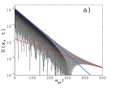
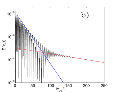
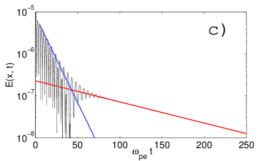
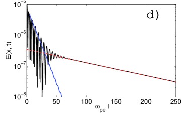
Figure 1: (Color online) LOKI simulation results for linear damping of EPWs. The amplitude of the perturbation’s electric field $E$ is plotted on a lin-log scale as a function of time $\omega_{pe}\,t$ for a wave with (a) $k\lambda_{De}=0.300$ and $\nu_{\rm ei,th}/\omega_{pe}=5\cdot 10^{-2}$; (b) $k\lambda_{De}=0.300$ and $\nu_{\rm ei,th}/\omega_{pe}=3\cdot 10^{-1}$; (c) $k\lambda_{De}=0.425$ and $\nu_{\rm ei,th}/\omega_{pe}=7\cdot 10^{-2}$; and (d) $k\lambda_{De}=0.425$ and $\nu_{\rm ei,th}/\omega_{pe}=2.1\cdot 10^{-1}$ In all cases, $\nu_{\rm ei,\max}/\nu_{\rm ei,th}=100$. In the first phase, following a brief transient of $\omega_{pe}t~{}\simeq 10$, one observes the damping of the standing EPW, whose finite real frequency leads to the oscillation of the amplitude. In a second phase, an initially small ’collisional’ or ’entropy’ mode with weaker damping survives. Zero real frequency of this ’collisional’ mode implies no oscillation of the amplitude. The red lines are an exponential decay fit to the observed entropy mode based on simulation data late in time. That behavior is extrapolated to all times and subtracted from the total field which allows more accurate determination of the frequency and damping of the EPW. The exponential decay fit to the EPW is shown by the blue lines.

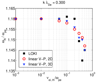
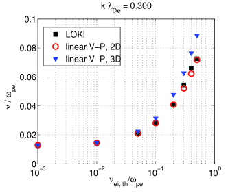
Figure 2: Effect of collisions on linear EPW damping for $k\lambda_{De}=0.300$. LOKI simulation results (black square markers) are compared to the linearized Vlasov-Poisson system with electron-ion collisional scattering in the two- and three-dimensional velocity space (red circles and blue triangles respectively). For all results, the maximum collision rate was capped at $\nu_{\rm ei,\max}/\nu_{\rm ei,th}=100$. Plotted are (a) the real frequency, $\omega_{R}/\omega_{pe}$, and (b) the damping rate, $\nu/\omega_{pe}$, as a function of the normalized thermal electron-ion collision frequency $\nu_{\rm ei,th}/\omega_{pe}$. Note the very good agreement between the predictions from the linearized Vlasov-Poisson system with collisions in 2D velocity space and the LOKI simulations. Note also that the maximum relative difference on the damping rate between results for 2D and for 3D velocity scattering is only $20\%$ and occurs at very high collisionality.

Figures 1.a and 1.b show time traces from LOKI simulations of the amplitude of the EPW for $k\lambda_{De}=0.300$, while Figs. 1.c and 1.d show time traces for $k\lambda_{De}=0.425$. Figures 1.a to 1.d have $\nu_{ei,th}=5\cdot 10^{-2}$, $3\cdot 10^{-1}$, $7\cdot 10^{-2}$ and $2.1\cdot 10^{-1}$ respectively. In all cases, the velocity dependent collisionality $\nu_{ei}(v)$ has been capped at $\nu_{\rm ei,\max}=\nu_{ei}(\bar{v})=100\,\nu_{\rm ei,th}$, corresponding to $\bar{v}=0.215\,v_{\rm th\,e}$. In the LOKI simulations, the velocity $v_{c}=6\,v_{\rm th\,e}$ (the velocity beyond which $\nu_{ei}(v)$ is smoothly ramped down to zero as it approaches $v_{\max}$). Note for all cases that, once the oscillatory EPW has damped out, an initially small ’collisional’ mode with weaker damping and zero real frequency survives. This collisional mode, subsequently referred to as the entropy mode Brantov et al. (2004), is not observed for zero collisionality. In these figures, presenting waves in the linear regime, the decay of the EPW is as expected well fit with an exponential decay. The entropy mode appears as well to present a constant exponential decay rate. As will be discussed in Sec. III.5, this constant decay rate of the entropy mode is a consequence of the grid resolution at low velocity. The EPW results from LOKI, requiring significantly less fine velocity grids to ensure convergence, are however very well resolved. When analyzing the LOKI results, the constant exponential decay rate of the entropy mode evolution at later times is extrapolated and subtracted from the time traces at earlier times, enabling a more accurate determination of the frequency and damping of the EPW. The time interval over which the EPW frequency and damping are calculated depends on the total damping rate; more accuracy is possible at lower rates, with better than 1% at $k\lambda_{De}=0.300$ and $\nu_{ei,th}=0.05$ but less than 3% at $k\lambda_{De}=0.425$ and $\nu_{ei,th}=0.5$.

Real frequencies $\omega_{R}$ and damping rates $\nu$ of the EPW for $k\lambda_{De}=0.300$, obtained with both LOKI and the numerical solution of the system (25)-(30) for different collision frequencies $\nu_{\rm ei,th}/\omega_{pe}=0$ to $5\cdot 10^{-1}$, are summarized in Fig. 2. Numerical solutions to the linearized Vlasov-Poisson system (18)-(21) for collisions in 3D velocity space instead of 2D are also shown. This plot provides an assessment of the effect on the frequency and damping of the restriction of the collisional scattering to two velocity dimensions. Over all the cases considered, the maximum relative difference of the linear damping rate between the results obtained with the 2D and 3D velocity space collision operator is only $20\%$ and occurs at high collisionality.

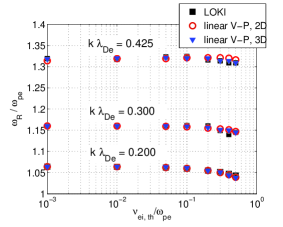
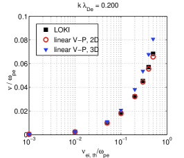
Figure 3: Effect of collisions on real frequency $\omega_{R}$ and damping rate $\nu$ of an EPW. Plotted are results from LOKI simulations (black square markers) as well as from the linearized Vlasov-Poisson system of equations with collisions in both 2D and 3D velocity space (red circles and blue triangles respectively). In (a), the frequency dependence for $k\lambda_{De}=0.200,0.300,\rm and\,0.425$ is shown. In (b) and (c), the damping rate for $k\lambda_{De}=0.200$ and $k\lambda_{De}=0.425$ are shown respectively.

The effect of collisions on the frequency and damping of EPWs was also studied with simulations with $k\lambda_{De}=0.425$, for which the collisionless linear Landau damping is larger than at $k\lambda_{De}=0.300$ (phase velocity is $v_{\phi}/v_{\rm th\,e}=3.100$ for $k\lambda_{De}=0.425$ instead of $v_{\phi}/v_{\rm th\,e}=3.867$ for $k\lambda_{De}=0.300$, see Table 1), as well as with simulations with $k\lambda_{De}=0.200$, for which the collisionless linear Landau damping is negligible (corresponding phase velocity $v_{\phi}/v_{\rm th\,e}=5.320$, see Table 1). Figure 3 shows the results for the frequency and damping as a function of the collision rate. In Fig. 3.a, the EPW frequency as a function of the collision rate $\nu_{ei,th}$ is shown for all the three cases: $k\lambda_{De}=0.200$, $0.300$, and $0.425$. Both the results from LOKI and from the linearized set are shown. The EPW damping rates from LOKI and the linearized set are shown in Fig. 3.b and 3.c for $k\lambda_{De}=0.200$ and $0.425$ respectively.

III.3 Approximate Analytic Solutions for Collisional Damping of EPWs

The electron-ion collision rate $\nu_{\rm ei,th}$ is typically much smaller than the collisionless Landau damping rate $\nu_{L}$ of EPWs. However, in very dense, high $Z$, or low temperature plasmas, for which $\nu_{ei,th}$ approaches $\omega_{pe}$, or for very high phase velocity waves, i.e. such that $v_{\phi}\gg v_{th,e}$ in which case Landau damping is negligibly small, $\nu_{ei,th}$ can be larger than the Landau damping rate $\nu_{L}$. Excitation of very high phase velocity EPWs may occur in Forward Stimulated Raman Scattering (FSRS) or in two-plasmon decay for which Landau damping of one of the decay EPWs is negligible. For weak collisions, Refs. Auerbach (1977) and Callen (2014) found that collisions do not affect the magnitude of Landau damping but do cause irreversible dissipation on a long time scale; thus plasma wave echos may be suppressed.Su and Oberman (1968)

Collisional damping of EPWs, resulting from the loss of momentum of the electrons oscillating in the field of the wave, can be obtained from the following set of fluid equations that represent the electron dynamics in an EPW:

$$\frac{d_{e}n_{e}}{dt}+n_{e}\nabla\cdot\vec{u}_{e}=0,$$ (33)

$$m_{e}n_{e}\frac{d_{e}\vec{u}_{e}}{dt}=e\,n_{e}\nabla\phi-\nabla p_{e}-m_{e}n_{e}\nu_{e}^{D}\left(\vec{u}_{e}-\vec{u}_{i}\right),$$ (34)

$$\frac{d_{e}}{dt}\left(\frac{p_{e}}{n_{e}^{\gamma_{e}}}\right)=0,$$ (35)

$$-\nabla^{2}\phi=-4\pi e\left(n_{e}-\sum_{i}N_{i}Z_{i}\right).$$ (36)

Note in particular the drag term on the right hand side of Eq. (34), resulting from momentum exchange due to electron-ion pitch angle scattering.Braginskii (1965) In the system (33)-(36), the operator $d_{e}/dt=\partial/\partial t+\vec{u}_{e}\cdot\nabla$ stands for the convective derivative along the mean electron velocity flow $\vec{u}_{e}$. The variables $n_{e}$ and $p_{e}$ respectively stand for the density and pressure of the electrons. The sum on the right hand side of Eq. (36) is again over all ion species $i$, assumed fixed, with uniform density $N_{i}$ and charge $Z_{i}e$, with overall charge neutrality assumed, $N_{e}=\sum_{i}N_{i}Z_{i}$, $N_{e}$ being the average electron density. Fixed ions imply that their average velocity $\vec{u}_{i}=0$. The parameter $\gamma_{e}=(d+2)/d$ stands for the adiabatic index, $d$ being the effective dimensionality of velocity space for the equation of state. Finally, the friction coefficient is denoted $\nu_{e}^{D}$. For three-dimensional pitch-angle scattering, $D=3$, and the friction rate $\nu_{e}^{D=3}=\nu_{ei}^{\rm brag}=1/\tau_{e}^{\rm brag}=[4/(3\sqrt{2\pi})]\,\nu_{ei,th}\simeq 0.532\,\nu_{ei,th}$, where $\nu_{ei}^{\rm brag}$ is the electron-ion collision frequency as defined by Braginski.Braginskii (1965) For two-dimensional scattering, $D=2$, and $\nu_{e}^{D=2}=\sqrt{\pi/8}\,\nu_{ei,th}\simeq 0.627\,\nu_{ei,th}$. These friction coefficients $\nu_{e}^{D}$ are derived by evaluating the drag $\vec{R}_{ei}=-m_{e}n_{e}\nu_{e}\vec{u}_{e}=-m_{e}\int d^{D}v\,\vec{v}\,C_{ei}f_{\rm SM}$ on a linearized shifted Maxwellian electron distribution $f_{SM}=f_{M}(1+\vec{v}\cdot\vec{u}_{e}/v_{\rm th\,e}^{2})$, with $f_{M}$ given by Eq. (22) and the collision operator $C_{ei}$ by Eq. (3). Note that $\nu_{e}^{D=2}>\nu_{e}^{D=3}$, and, thus, the fluid equations find the EPW collisional damping is stronger in 2D than in 3D. Yet, the effect of collisions on the damping rate observed in the simulations is stronger for $D=3$ than for $D=2$. In Appendix B, we will show that the fluid equation damping rate is about twice the correct value although the scaling with collision frequency is correct. The problem arises in the fact the the drag term is strongly weighted by velocities, $v\sim 0$, whereas, done correctly, velocities $\sim 0.2<v<1$ contribute the most. The weighting by higher velocity is stronger in 3D.

The system (33)-(36) can then be linearized with respect to small fluctuations $\delta n_{e}$, $\delta\vec{u}_{e}$ and $\delta p_{e}$ around the corresponding uniform background electron quantities, i.e. density $N_{e}$, zero background velocity $\vec{U}_{e}=0$, and background pressure $P_{e}=N_{e}T_{e}$ respectively, where $T_{e}$ is the background temperature. Assuming plane wave fluctuations with frequency $\omega$ and wavenumber $k$, one obtains a dispersion relation for the real frequency $\omega_{R}$ of EPWs given by the Bohm-Gross relation

$$\omega_{R}=\omega_{\rm BG}=\omega_{pe}\sqrt{1+\gamma_{e}(k\lambda_{De})^{2}}$$ (37)

and a corresponding damping rate

$$\nu_{\rm coll}=(\omega_{pe}/\omega_{R})(\nu_{e}^{D}/2)\simeq\nu_{e}^{D}/2,$$ (38)

provided $k\lambda_{De}\ll 1$ and $\nu_{e}^{D}\ll\omega_{pe}$. For weakly collisional plasma, i.e. $k\lambda_{ei}\gg 1$, with $\lambda_{ei}=v_{\rm th\,e}/\nu_{ei,th}$ the thermal electron-ion mean free path, the effective dimensionality for estimating $\gamma_{e}$ is $d=1$, so that $\gamma_{e}=3$. For a strongly collisional plasma, i.e. $k\lambda_{ei}\ll 1$, $d=D$, so that $\gamma_{e}=5/3$ for three-dimensional velocity space $D=3$, while $\gamma_{e}=2$ for $D=2$. This strongly collisional fluid equation result for the frequency and damping rate in the case $D=3$ is recovered in Appendix B.1 by solving a dispersion relation obtained from the $l=0,1$ equations in the system of Eqs. (18)-(21) in the limit that $k\lambda_{De}\ll 1$ and $\nu_{ei,th}\ll\omega_{pe}$. The corresponding two-dimensional ($D=2$) fluid result for the collisional damping can be recovered as well from the $m=0,1$ equations in the system (25)-(30), as shown in Appendix B.2. The solution to the dispersion that agrees with the fluid dispersion is obtained by Taylor expanding the integrand in the presumably small parameter $\nu_{ei,th}/\omega_{pe}$. However, this damping rate is about twice the Vlasov simulation damping rate attributable to the direct effect of collisions shown in Fig. 4. In Appendix  B.2, we numerically obtain the correct solution to the dispersion relation and show that it agrees very well with the kinetic simulations.

III.4 Analysis of results

In Figure 4, the Vlasov simulation results for the collisional part of the damping rate are shown as a function of $\nu_{ei,th}/\omega_{pe}$ for the different values of $k\lambda_{De}$. The collisional component of the damping rate is estimated by subtracting the collisionless Landau damping rate $\nu_{L}$ (found analytically, see Table 1, or equivalently taken from LOKI simulation at small $\nu_{ei,th}$) from the total damping rate (shown in Figs. 2 and 3) obtained from the simulations. Figure 4.a shows no discernable $k\lambda_{De}$ dependence of the collisional damping component for $\nu_{ei,th}/\omega_{pe}<0.1$. For $\nu_{ei,th}/\omega_{pe}>0.1$, the EPWs with larger $k\lambda_{De}$ have a lower collisional damping rate component than the higher phase velocity waves as expected from the factor $\omega_{pe}/\omega_{R}$ in the fluid equation result given by Eq. (38).

Note that the collisionless phase velocities are $v_{\phi}/v_{\rm th\,e}=5.320$, $3.867$ and $3.100$ for $k\lambda_{De}=0.200$, $0.300$ and $0.425$ respectively (see again Table 1). Figure 3.a shows that the real frequency $\omega_{R}$ of the EPWs decreases – and thus the phase velocity decreases as well – with increasing $\nu_{ei,th}$. The Landau damping estimated with the frequency $\omega_{R}$ modified by finite collisionality should thus increase with $\nu_{ei,th}$ and consequently lower the collisional component to the damping.

In the following, we consider the effect of arbitrarily setting some terms to zero in the linearized set of equations (25)-(30) for the Vlasov-Poisson system with collisions in two-dimensional velocity space. For this study the particular case $k\lambda_{De}=0.425$ is considered. In one limit, the effect of only collisions, neglecting thermal corrections to the frequency as well as any wave-particle resonance effects (in particular Landau damping), is studied by removing the coupling of $\delta f_{c_{1}}$ to $\delta f_{c_{0}}$ and to $\delta f_{c_{2}}$ but keeping the coupling of $\delta f_{c_{0}}$ to $\delta f_{c_{1}}$. That is, Eq. (25) is left unchanged and Eq. (26) is replaced by Eq. (39):

$$\frac{\partial\,\delta\!f_{c,1}}{\partial t}-ikv\,\phi\,f_{M} =-\nu_{\rm ei}(v)\,\delta\!f_{c,1}.$$ (39)

Keeping the coupling of $\delta f_{c_{1}}$ to $\delta f_{c_{0}}$ would introduce an unphysical resonance at $\omega=kv/\sqrt{3}$ in 3D or $\omega=kv/\sqrt{2}$ in 2D as occurs in Eq. (61) and Eq. (63) for 3D and 2D respectively. The results of that approximation yield the drag-limit damping rate $\nu_{2dDL}$, shown by the red diamonds in Fig. 5 and are about 1/2 the imaginary part of Eq. (64) as explained in Appendix B.

In a complementary limit, all terms and equations of the system (25)-(30) are kept except for the collision term on the right hand side of the evolution equation for $\delta f_{c_{1}}$, effectively eliminating drag but keeping Landau damping. That is, Eq. (25) is left unchanged and Eq. (26) is replaced by Eq. (40):

$$\frac{\partial\,\delta\!f_{c,1}}{\partial t}+ikv\,\left(\delta\!f_{c,0}+\frac{\delta\!f_{c,2}}{2}\right)-ikv\,\phi\,f_{M} =0.$$ (40)

The results of that approximation yield the no-drag damping rate $\nu_{2dND}$, shown by the blue triangles in Fig. 5. This latter approximation is thus meant to include Landau damping and the effect of collisions on Landau damping but not collisional damping resulting from drag on the non-resonant electrons, at the origin of the damping derived in Sec. III.3.

The sum of the damping from the two above-mentioned approximations yields the green circles in Fig. 5, which define a set of damping rates which are close but somewhat larger than the values from the LOKI simulations shown by the black squares in this same figure. The numerical solution of the full linearized set (25)-(30) agrees very well with LOKI results as was shown in Figs. 2 and 3. Self-consistency is one difficulty in making the comparison in Fig. 5 between the green data points and the simulation results. As already discussed above, Landau damping depends on the phase velocity $v_{\phi}=\omega_{R}/k$ which is determined by the solution to the linearized set that has been modified by dropping terms. Analysis of results for the real frequency $\omega_{R}$ without the collision term in the equation for $\delta f_{c_{1}}$ shows that it is nearly the same as the LOKI frequency, $\omega_{R,{\rm LOKI}}$, so the blue triangles are unaffected by a $v_{\phi}$ difference. The real frequency $\omega_{R}$ in the purely collisional case is however quite different, essentially $\omega_{R}=\omega_{pe}$, because there are no thermal contributions to the dispersion. Using the relation for the collisional damping from Eq. (64), $\nu_{\rm coll}=\sqrt{\pi/2}{\nu_{ei,th}}/{4\omega_{R}}$, we reduced the collision damping contribution to the total damping by multiplication with the factor $\omega_{pe}/\omega_{R,{\rm LOKI}}$, which brings the results [red open circles in Fig. 5] close to the LOKI results. Here $\omega_{R,{\rm LOKI}}$ is the frequency in the corresponding LOKI simulation. The ansatz that collisions would reduce Landau damping, that is, that the blue triangles would define a decreasing sequence of points in Fig. 5, is not borne out by this analysis perhaps because the phase velocity in the linearized system decreases as the collision rate increases.

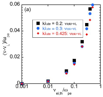
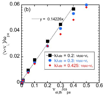
Figure 4: The collisional component $\nu-\nu_{L}$ of the EPW damping rate obtained from the LOKI simulations is shown as a function of $\nu_{ei,th}/\omega_{pe}$ for the cases $k\lambda_{De}=0.200$,$k\lambda_{De}=0.300$, and $k\lambda_{De}=0.425$ on (a) a logarithmic scale and (b) a linear scale for the collisionality. To obtain the collisional damping component, the calculated value $\nu_{L}$ of the collisionless Landau damping (see Table 1) was subtracted from the total damping obtained from the simulations. The collisional component for $k\lambda_{De}=0.200$ follows a linear relation wrt. $\nu_{ei,th}/\omega_{pe}$. The results for the higher $k\lambda_{De}$ values fall below this line as expected from Eq. (38).

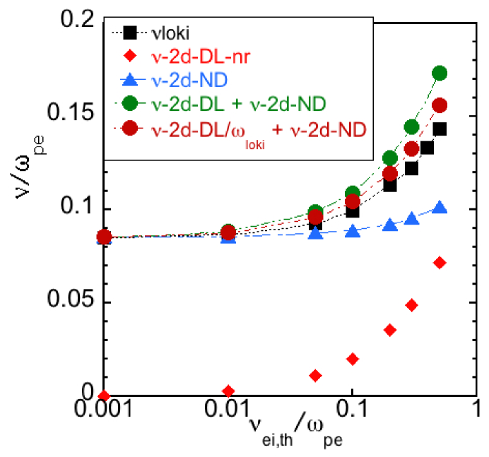
Figure 5: Damping rates of EPWs for $k\lambda_{De}=0.425$. Shown are the results from LOKI simulations (black squares) and from different limits of the linearized Vlasov-Poisson system (details given in text): collisions but without thermal and resonant effects (red diamonds); setting the collisional term to zero in the equation for $\delta f_{c_{1}}$ (blue triangles); the sum of red diamonds and blue triangles (green circles); and the sum of the blue triangles and red diamonds, the latter corrected by the factor $\omega_{pe}/\omega_{R,{\rm LOKI}}$, with $\omega_{R,{\rm LOKI}}$ the real frequency obtained from the corresponding LOKI simulations (red circles).

III.5 Entropy mode

The entropy mode can be conveniently modeled in the so-called diffusive limit. The focus here is on the case of electron-ion pitch angle scattering in two-dimensional velocity space, $D=2$, relevant to the results obtained by the LOKI code. The starting point are Eqs. (25) and (26) for the two coefficients $\delta f_{c,0}(v)$ and $\delta f_{c,1}(v)$ of the fluctuating part of the electron distribution decomposed in polar Fourier modes (here in normalized units):

$$\frac{\partial\,\delta\!f_{c,0}}{\partial t}+\frac{ikv}{2}\delta f_{c,1}=0,$$ (41)

$$ikv\,(\delta f_{c,0}-\phi\,f_{M})=-\nu_{\rm ei}(v)\,\delta f_{c,1}.$$ (42)

In Eq. (42), the term $\partial\,\delta\!f_{c,1}/\partial t$, related to electron inertia, has been neglected with respect to the collision term on the right hand side of this equation, under the assumption that the perturbation varies slowly on the electron-ion collision time scale $\nu_{ei,th}$. Also, the coupling to $\delta\!f_{c,2}$ has been neglected in this same equation, which is justified under the further assumption $k\lambda_{\rm ei}\ll 1$, corresponding to the collisional limit. The ratio of consecutive coefficients indeed scales as $|\delta f_{c,m+1}/\delta f_{c,m}|\sim k\lambda_{\rm ei}$. Eliminating $\delta f_{c,1}$ from the system (41) and (42) and furthermore making use of the Poisson equation (30) leads to an effective equation for the component $\delta f_{c,0}(v,t)$:

$$\frac{\partial\,\delta\!f_{c,0}}{\partial t}=-\frac{(kv)^{2}}{2\,\nu_{\rm ei}(v)}\delta f_{c,0}-\pi\frac{v^{2}f_{M}(v)}{\nu_{\rm ei}(v)}\int_{0}^{+\infty}v\,dv\,\delta\!f_{c,0}\quad,$$ (43)

referred to as the diffusive approximation.Albritton (1983); Epperlein (1994)

The evolution equation (43) has a spectrum of eigenmodes with fixed damping rate $\nu\in\mathbb{R}_{+}$:

$$\delta f_{\nu}(v,t)=\delta\hat{f}_{\nu}(v)e^{-\nu t}=\left[\pi\frac{v^{2}f_{M}(v)}{\nu_{\rm ei}(v)}\frac{\mathcal{P}}{\nu-(kv)^{2}/[2\nu_{\rm ei}(v)]}+\frac{A}{v_{0}}\,\delta(v-v_{0})\right]e^{-\nu t}.$$ (44)

In Eq. (44), the velocity $v_{0}\in\mathbb{R}_{+}$ is defined such that $\nu=(kv_{0})^{2}/[2\nu_{\rm ei}(v_{0})]$, or equivalently $v_{0}/v_{\rm th\,e}=[2\,\nu\,\nu_{ei,th}/(kv_{\rm th})^{2}]^{1/5}$. The symbol $\mathcal{P}$ appearing in the first term on the right hand side of Eq. (44) indicates that the resonance at $v_{0}$ in the denominator is to be handled in the sense of the Cauchy principal value when carrying out velocity integrals of this term. The coefficient $A$ multiplying the Dirac function centered at $v_{0}$ in the second term on the right hand side of Eq. (44) is given by

$$A=1-\pi\,\mathcal{P}\int_{0}^{\infty}dv\frac{v^{3}f_{M}(v)}{\nu_{\rm ei}(v)}\frac{1}{\nu-(kv)^{2}/[2\nu_{\rm ei}(v)]}.$$ (45)

One can easily check by substitution that Eqs. (44) and (47) provide a solution to (43) for any $\nu\in\mathbb{R}_{+}$. The spectrum of the diffusive equation is thus purely real, positive and continuous. The associated eigenmodes of the form (44) are clearly singular at $v=v_{0}$. One may note the analogy between these eigenmodes to the diffusive Eq. (43) and the singular Van Kampen eigenmodes to the collisionless Vlasov-Poisson system,Kampen (1955) the corresponding spectra in this latter case being also continuous, however purely imaginary (reflecting undamped modes). The fact that the eigenmodes of Eq. (43) are singular and the associated spectrum is continuous results from the fact that only pitch angle scattering collisions have been considered here. Accounting for thermalization of the electrons through self-collisions would lead to a related diffusive term involving a second order derivative in Eq. (43). The nature of the equation would consequently be modified, leading to a discrete spectrum and associated non-singular eigenmodes.

For a smooth initial perturbation $\delta f_{c,0}(v,t=0)$, such as the sinusoidal density perturbation considered for the EPW simulations and given by (31), the evolution predicted by the diffusive approximation (43) will be an infinite superposition over the continuous spectra of eigenmodes of the form (44) with different values of $\nu$: $\delta f_{c,0}(v,t)=\int_{0}^{\infty}d\nu\,C(\nu)\,\delta\hat{f}_{\nu}(v)\,e^{-\nu t}$, with $C(\nu)$ the coefficient function of the decomposition. The evolution of such a solution will thus not present a single exponential decay, it being a continuous superposition of modes with different damping rates $\nu$.

A typical solution to the diffusive approximation equation (43) for an initial perturbation of the form (31) is given in Figure 6, for a perturbation with $k\lambda_{De}=0.300$, collisionality $\nu_{\rm ei,th}/\omega_{pe}=1\cdot 10^{-1}$ and $\nu_{\rm ei,\max}/\nu_{\rm ei,th}=100$. This numerical result was obtained with a velocity amplitude grid resolution of $n_{v}=256$ and $v_{\rm max}/v_{\rm th\,e}=7$. Plotted is the amplitude of the electrostatic field as a function of time. Note that the evolution is purely damped, i.e. non-oscillatory, reflecting, as expected, that the diffusive approximation model does not reproduce the EPW dynamics. Furthermore, the perturbation is very strongly damped at early times, due to the decay of the eigenmode components $C(\nu)\delta f_{\nu}$ related to high values of $\nu$. These highly damped eigenmodes are singular at a high velocity value $v_{0}/v_{\rm th\,e}=[2\,\nu\,\nu_{ei,th}/(kv_{\rm th})^{2}]^{1/5}$, such that corresponding effective collisionality is low, $\nu_{\rm ei}(v_{0})\ll\nu$, and consequently the effective mean free path is large, i.e. $kv_{0}/\nu_{\rm ei}(v_{0})\gg 1$. These scalings violate the assumptions made in deriving the diffusive model. At later times, the remaining perturbation from the diffusive approximation result decays at a much slower rate, corresponding to the decay of the eigenmode components $C(\nu)\delta f_{\nu}$ with low values of $\nu$. These weakly damped eigenmodes are singular at a low velocity value $v_{0}$, with a high corresponding effective collisionality $\nu_{\rm ei}(v_{0})\gg\nu$ and a short effective mean free path, $kv_{0}/\nu_{\rm ei}(v_{0})\ll 1$. These latter scalings are in agreement with the assumptions of the diffusive model.

Also shown in Fig. 6 is the evolution of the linearized Vlasov-Poisson system with collisions given by Eqs. (25)-(30), with oscillating EPW evolution at early times and purely damped entropy mode evolution at later times. This numerical result was obtained with a velocity amplitude grid resolution of $n_{v}=256$, $v_{\rm max}/v_{\rm th\,e}=7$ and maximum $M=8$ polar Fourier modes. Note how the later time evolution is perfectly reproduced by the solution to the diffusive approximation equation. This agreement at later times is expected, given that, as already mentioned, it corresponds to the evolution which is within the limits of validity of the reduced diffusive approximation model.

Subtracting over the full simulation time the entropy mode evolution provided by the diffusive approximation from the evolution of the full Vlasov-Poisson system with collisions provides the evolution of the EPW with a single exponential decay rate over a very long simulation time, as shown in Fig. 6. Such a subtraction technique enables a very accurate estimate of the real frequency and damping rate for the EPW and was applied for all results presented in figures 2 and 3.

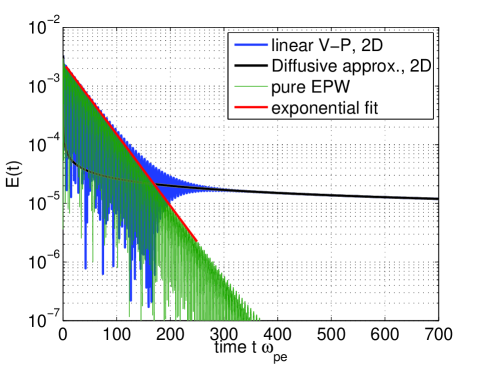
Figure 6: Solutions to both the linearized Vlasov-Poisson system with collisions (25)-(30) (blue line) and the diffusive approximation equation (43) (black) for the same initial sinusoidal density perturbation in case of 2D velocity scattering. Plotted is the evolution of the perturbation amplitude as a function of time in lin-log scale. Subtracting the two solutions solution (black from blue curve) provides the time evolution of the pure EPW (green), presenting an exponential damping over a much longer time. A fit (red) to the envelope of this latter curve provides a very accurate estimate for the decay rate of the EPW. In this example, $k\lambda_{De}=0.300$, $\nu_{\rm ei,th}/\omega_{pe}=1\cdot 10^{-1}$ and $\nu_{\rm ei,\max}/\nu_{\rm ei,th}=100$.

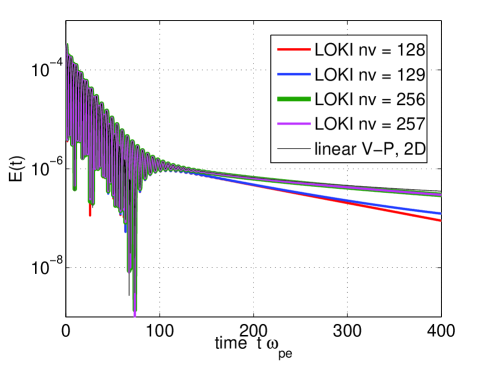
Figure 7: Convergence study in case of the entropy mode for LOKI simulations. Shown is the time evolution of the mode amplitude for the case $k\lambda_{De}=0.300$, $\nu_{ei,th}=5\cdot 10^{-1}\omega_{pe}$ and $\nu_{\rm ei,\max}=\nu_{ei,th}$, corresponding to $\bar{v}=v_{\rm th\,e}$. Resolution is simultaneously increased along both $v_{x}$ and $v_{y}$, with $n_{v_{x}}=n_{v_{y}}=128$, $129$, $256$, and $257$ grid points and keeping $v_{x,\max}=v_{y,\max}=v_{\max}=7\,v_{\rm th\,e}$ fixed. Also plotted is the corresponding result from the linearized Vlasov-Poisson system (25)-(30) in polar velocity coordinates, obtained with the following resolution ensuring convergence: $v_{\rm max}=7$, $n_{v}=128$ and maximum polar Fourier mode $M=8$.

The derivation of the reduced diffusive approximation model (43) in case of three-dimensional velocity scattering, $D=3$, can obviously also be carried out starting from Eqs. (18) and (19) for the evolution of the first two components $\delta f_{0}(v)$ and $\delta f_{1}(v)$ of the fluctuating part of the electron distribution decomposed in Legendre polynomials. The eigenmodes again define a purely real, positive, continuous spectrum $\nu\in\mathbb{R}_{+}$ with associated singular eigenmodes:

$$\delta f_{\nu}(v,t)=\delta\hat{f}_{\nu}(v)e^{-\nu t}=\left[\frac{2\pi}{3}\frac{v^{2}f_{M}(v)}{\nu_{\rm ei}(v)}\frac{\mathcal{P}}{\nu-(kv)^{2}/[6\nu_{\rm ei}(v)]}+\frac{A}{v_{0}^{2}}\,\delta(v-v_{0})\right]e^{-\nu t},$$ (46)

the coefficient $A$ being given in this case by

$$A=1-\frac{2\pi}{3}\,\mathcal{P}\int_{0}^{\infty}dv\frac{v^{4}f_{M}(v)}{\nu_{\rm ei}(v)}\frac{1}{\nu-(kv)^{2}/[6\nu_{\rm ei}(v)]}.$$ (47)

Let us finally address the convergence of the late time entropy mode evolution in the LOKI simulations. As already mentioned in Sec. III.2 when commenting on the results plotted in Fig. 1, the entropy mode evolution is not fully resolved in most LOKI simulations. This can be better understood based on the above discussion of the entropy eigenmodes (44) derived in the diffusive approximation. It has been shown that the late time evolution of the Vlasov-Poisson system with collisions is defined by the slowest decaying entropy eigenmodes which are singular at near zero velocity $v_{0}\ll v_{\rm th\,e}$. As these eigenmodes are very well represented by the diffusive approximation, which considers only poloidal Fourier modes $m=0$, $1$, they are nearly circularly symmetric and easily resolved when solving the linearized Vlasov-Poisson system in polar velocity coordinates, as considered for the system of Eqs. (25)-(30) ( e.g. the green curve in Fig. 6). However, the Cartesian velocity coordinate system used by LOKI is not appropriate for easily resolving the singular structure of weakly damped entropy eigenmodes in the vicinity of zero velocity, as the number of grid points in this region of velocity space with this representation is very limited for typical resolutions required for accurately evolving EPWs. Nonetheless, convergence of the LOKI simulation results with respect to increasing velocity resolution is illustrated in Figure 7. Plotted is the perturbation amplitude evolution of an initial sinusoidal density perturbation with $\delta n/N=1\cdot 10^{-4}$ (ensuring linear regime), $k\lambda_{De}=0.300$, $\nu_{ei,th}=5\cdot 10^{-1}\omega_{pe}$ and $\nu_{\rm ei,\max}=\nu_{\rm ei,th}$. The resolution along the $v_{x}$ and $v_{y}$ velocity directions were the same. In a series of computations, an increasing number of velocity grid points $n_{v}=128$, $129$, $256$, and $257$ were chosen. In all cases the maximum velocity grid value was set to $v_{x,\max}=v_{y,\max}=v_{\max}=7v_{\rm th\,e}$. For the lowest resolution, $n_{v}=128$, the early time EPW evolution is already fully converged. The later time entropy mode evolution presents however a constant exponential decay, illustrating that the simulation was only able to resolve some of the infinite number of weakly damped entropy eigenmodes located near zero velocity. As the velocity resolution is increased, additional weakly damped entropy eigenmodes are resolved by LOKI, and one consequently observes that the corresponding perturbation amplitude presents a time evolution with varying decay rate. For $n_{v}=256$ the LOKI result is thus nearly converged with the reference result provided by the linearized Vlasov-Poisson system in polar coordinates given by (25)-(30) over the simulation time $0<t\omega_{pe}<400$. Fig. 7, shows a significant effect on the entropy mode evolution for an odd number of grid points for which a grid point at the critical velocity point $(v_{x},v_{y})=(0,0)$ exists near the location of the weakest damped eigenmodes. Such a grid point at zero velocity is lacking for $n_{v}$ even.

IV Simulation Results of Nonlinear Landau Damping

The results presented in the previous sections addressed the linear regime of very small amplitude waves for which the linear EPW damping rate $\nu$ is much faster than the bounce frequency $\omega_{B}$ of an electron trapped in the potential well of the wave. The bounce frequency may be estimated with the deeply trapped estimate $\omega_{B}/\omega_{pe}=k\lambda_{De}\sqrt{e\phi_{0}/T_{e}}$, where $\phi_{0}$ is the finite amplitude of the electrostatic potential associated to the wave.

Without collisions, a wave initialized with amplitude $\phi_{0}$ such that $\omega_{B}>\nu$ will damp at the linear Landau rate $\nu_{L}$ only until the bounce time, $\tau_{B}\sim\omega_{Be}^{-1}$.O’Neil (1965); Morales and O’Neil (1972) After that, the electrostatic field and bulk electrons exchange energy back and forth, but without further net transfer to resonant particles and consequently there is no further Landau damping of the wave. In Fig. 8, the time history of a wave with amplitude $\delta n/N=0.1$ in a collisionless plasma shows the wave reaches such a stationary state, referred to as a BGK mode.Bernstein et al. (1957)

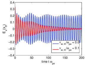
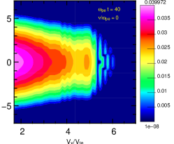
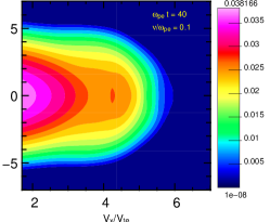
Figure 8: Results from the LOKI code of non-linear Landau damping. (left) The amplitude of the electrostatic field $E_{x}$ (longitudinal component) as a function of time $\omega_{pe}t$ for an EPW with $k\lambda_{De}=0.3$ and initial relative amplitude of the density perturbation $\delta n/N=0.1$. Results from both a simulation with zero collision rate (blue) and finite collision rate $\nu_{\rm ei,th}/\omega_{pe}=0.1$ (red) are shown. The electron distribution function as a function of velocity $v_{x}$ and $v_{y}$ averaged over $x$ in the resonant region is shown at $\omega_{pe}t=40$ (middle) for the collisionless case and (right) the collisional case with $\nu_{ei,th}=0.1$.

With strong collisions (in this case $\nu_{ei,th}/\omega_{pe}=0.1$), the wave continues to damp after a bounce time. Results of collisional effects on non-linear Landau damping obtained with the LOKI code are provided in Fig. 8, where the time trace of the longitudinal field $E_{x}$ at the position $x$ of the anti-node of the standing wave is shown for an initial relative amplitude of the density perturbation $\delta n/N=0.1$, both in the case of zero collision rate, and finite collision rate $\nu_{\rm ei,th}/\omega_{pe}=0.1$. The other parameters for the effective collision frequency $\bar{\nu}_{ei}(v)$ are $\nu_{\rm ei,\max}/\nu_{\rm ei,th}=100$ and $v_{c}/v_{\rm th\,e}=6$. The phase space resolutions are the same as for the linear Landau damping simulations. The physical parameters for the runs in Fig. 8 are in fact identical to the ones considered in Fig. 9 of Ref. Brunner (2009), except that the LOKI code considers a Lorentz collision operator restricted to 2D velocity space, while the results obtained in Ref. Brunner (2009) with a collisional version of the semi-Lagrangian SAPRISTI code that supports scattering in 3D velocity space. The LOKI and SAPRISTI results are nonetheless strikingly similar.

Also shown in Fig. 8 is the distribution of electrons in the resonant region of velocity space corresponding to these two cases. The addition of moderate collisions acts to isotropize the distribution of trapped electrons and reduces the marked oscillations along $v_{x}$ at the high velocity edge of the trapping regions where there are steep velocity gradients.

V Conclusions

Because a fully five dimensional phase space (2 space plus 3 velocity) is beyond the computational resources for continuum method solution to the Vlasov system of equations, we constructed LOKI with a four dimensional (2 space plus 2 velocity) algorithm. A simple pitch angle scattering operator in two-dimensional velocity space has been implemented in the LOKI code using a conservative, finite-difference discretization scheme. Despite the fact that the time integration scheme in LOKI is explicit (4th order Runge-Kutta), the CFL-type limit on the time step remains ’affordable’, even at the higher end of the relevant range of collision frequencies. A practical, approximate, analytical relation (see Eq. (57)) for estimating the CFL time limit related to the collision operator was derived and validated in Appendix A. The implementation has been successfully tested in the case of collisional effects on linear Landau damping, where results obtained with an alternative numerical approach were available for comparison. Results of non-linear Landau damping were obtained as well. An improved collision operator, corresponding to test particle collisions off a Maxwellian distribution, is under development. Although still restricted to two-dimensional velocity space, such an operator would account for thermalization effects, currently missing with the simple pitch angle scattering operator.

Landau damping and electron plasma waves constitute both fundamentally interesting plasma physics processes and the least complicated systems to study within the context of the Vlasov-Poisson system of equations. Here, we added the simplest collisional operator, electron-ion, pitch-angle scattering and examined the effects on EPWs of Landau and collisional damping. Despite its simplicity and its importance to basic plasma physics, Landau damping in the presence of electron scattering from the ions has received little attention. There have been several analytical theory papers motivated by early work on plasma waves echoesGould et al. (1967); Malmberg et al. (1968) and the effects of collisions on echoesBaker et al. (1968); Su and Oberman (1968). Recent semi-analytic work on EPW damping with collisionsBrantov et al. (2012) followed the approach in Sec. III.1.1, included self-collisions as well, but employed a time Fourier transform rather than direct numerical integration as done here.

The dependence of the collisional damping on $k\lambda_{De}$ that we found in Fig. 4 relies on the assumption that collisions do not ’disrupt’ Landau damping as we find the collisional damping merely by subtracting the collisionless Landau rate from the total damping. In Sec. III.4, we used the linearized equations expanded in a Fourier series obtained in Sec. III.1.2 but modified to exclude Landau damping in one limit and to exclude collisional damping in another limit. We examined the case $k\lambda_{De}=0.425$ with a strong Landau damping because of its low phase velocity, $v_{\phi}=3.1v_{\rm th\,e}$ where electron-ion collision effects on the wave-particle resonance should be strongest. As Fig. 5 shows, we found that these equations show no decrease in Landau damping as $\nu_{ei,th}$ increases, in fact, a slight increase. The sum of the collisional damping and the Landau damping from this modified set of equations shows a total damping similar to but slightly bigger than the LOKI results and the results from the full linearized set. The full set and the LOKI results are in excellent agreement as shown in Fig. 3c. Thus, the separation of processes was not completely successful.

An important and unexpected outcome of our simulations and analysis is that the collisional damping of EPWs is less than obtained from a linearized set of fluid equations where the electron-ion momentum exchange term is the source of the damping. The collision term in momentum moment of the Fokker-Planck equation, Eq. (34), includes a collision rate, $\nu_{e}^{D}$, that is strongly weighted by low velocities which leads in turn to a EPW collisional damping rate, $\nu_{coll}\simeq\nu_{e}^{D}/2$ whereas the correct kinetic treatment in Appendix B shows that, for EPWs, the effective rate should be weighted by much higher but still bulk velocity electrons.

The LOKI simulations also revealed the presence of entropy modes, that is, non-oscillatory, weakly-damped modes. The nature of these modes is sensitive to the absence of collisional thermalization effects. Thus, in this manuscript, we emphasize only the need to account for their presence when extracting EPW damping rates.

We briefly studied the effect of collisions on nonlinear processes that rely on particle trapping. This subject will be examined more fully in subsequent publications for both EPWs and ion acoustic waves.

VI Acknowledgments

We are pleased to acknowledge valuable discussions with T. Chapman and B. I. Cohen. This work was performed under the auspices of the U.S. Department of Energy by Lawrence Livermore National Laboratory under Contract DE-AC52-07NA27344 and funded by the Laboratory Research and Development Program at LLNL under project tracking codes 12-ERD-061 and 15-ERD-038. Computing support for this work came from the Lawrence Livermore National Laboratory (LLNL) Institutional Computing Grand Challenge program.

Appendix A Discretization with finite differences

Here we briefly discuss the discretization of the pitch angle collision operator (14) using fourth-order accurate conservative finite differences. For convenience we reproduce the operator here

$$C_{ei}f= \,\nu_{\rm ei,th}\left\{\frac{\partial}{\partial v_{x}}\left[\left(\frac{v_{\rm th\,e}}{v}\right)^{3}v_{y}\left(v_{x}\frac{\partial f}{\partial v_{y}}-v_{y}\frac{\partial f}{\partial v_{x}}\right)\right]\right.$$

$$\hskip 22.76219pt\left.-\frac{\partial}{\partial v_{y}}\left[\left(\frac{v_{\rm th\,e}}{v}\right)^{3}v_{x}\left(v_{x}\frac{\partial f}{\partial v_{y}}-v_{y}\frac{\partial f}{\partial v_{x}}\right)\right]\right\}.$$

It will be convenient to express this operator in the generic form

$$C_{ei}f=\frac{\partial}{\partial v_{x}}\left(a\frac{\partial f}{\partial v_{x}}+b\frac{\partial f}{\partial v_{y}}\right)+\frac{\partial}{\partial v_{y}}\left(c\frac{\partial f}{\partial v_{x}}+d\frac{\partial f}{\partial v_{y}}\right)$$ (48)

with $a$, $b$, $c$, and $d$ defined respectively by

$$a =-\bar{\nu}_{ei}(v)\,v_{y}^{2},$$

$$b =+\bar{\nu}_{ei}(v)\,v_{x}v_{y},$$

$$c =+\bar{\nu}_{ei}(v)\,v_{x}v_{y},$$

$$d =-\bar{\nu}_{ei}(v)\,v_{x}^{2},$$

where the actual velocity dependent collision frequency $\bar{\nu}_{ei}(v)$ implemented in LOKI is given explicitly in Equation (55).

The conservative treatment of the conservative unmixed and mixed derivatives in Eq. (48) will be described below. Throughout the discussion we will use standard notation for the divided difference operators in the $v_{x}$ direction:

$$D_{+,v_{x}}f_{i,j} =\frac{f_{i+1,j}-f_{i,j}}{\Delta v_{x}},$$

$$D_{-,v_{x}}f_{i,j} =\frac{f_{i,j}-f_{i-1,j}}{\Delta v_{x}},$$

$$D_{0,v_{x}}f_{i,j} =\frac{f_{i+1,j}-f_{i-1,j}}{2\Delta v_{x}}.$$

Likewise for the $v_{y}$ direction:

$$D_{+,v_{y}}f_{i,j} =\frac{f_{i,j+1}-f_{i,j}}{\Delta v_{y}},$$

$$D_{-,v_{y}}f_{i,j} =\frac{f_{i,j}-f_{i,j-1}}{\Delta v_{y}},$$

$$D_{0,v_{y}}f_{i,j} =\frac{f_{i,j+1}-f_{i,j-1}}{2\Delta v_{y}}.$$

A.1 Unmixed derivative operators

Consider the unmixed derivative in the $v_{x}$-direction, in particular, the term $\frac{\partial}{\partial v_{x}}(a\frac{\partial f}{\partial v_{x}})$, the formulation in the $v_{y}$-direction being a straightforward extension. Following the discussion in Ref. Henshaw (2006), conservative discretizations can be obtained. Begin by defining coefficients $\beta_{k}$ to satisfy the identity

$$\frac{\partial w}{\partial{v_{x}}}\left(v_{x}\pm\frac{\Delta v_{x}}{2},v_{y}\right)=$$

$$\quad D_{\pm,v_{x}}\left[\sum_{k=0}^{m}\beta_{k}\Delta v_{x}^{2k}(D_{+,v_{x}}D_{-,v_{x}})^{k}\right]w\left(v_{x},v_{y}\right)$$

$$\quad+{\mathcal{O}}(\Delta v_{x}^{2m+2}),$$ (49)

for infinitely differentiable functions $w$. For our purposes we are seeking fourth-order accurate discretizations and therefore need only $\beta_{0}$ and $\beta_{1}$. However, as discussed in Ref. Fornberg (1996), the $\beta$ coefficients can be evaluated to arbitrary order using

$$\xi=\sin(\xi)\left[\sum_{k=0}^{\infty}\beta_{k}(-4\sin^{2}(\xi))^{k}\right],$$

giving $\beta_{0}=1$, $\beta_{1}=-\frac{1}{24}$, $\beta_{2}=\frac{3}{640}$, $\beta_{3}=-\frac{5}{7168}$, $\beta_{4}=\frac{35}{294912}$, and so forth. Now define the following operators:

$${\mathcal{D}}_{\pm,v_{x}}=D_{\pm,v_{x}}\left[\sum_{k=0}^{\infty}\beta_{k}\Delta v_{x}^{2k}(D_{+,v_{x}}D_{-,v_{x}})^{k}\right],$$

which can be interpreted as an infinite-order-accurate representation of the derivative at the “half points” [e.g. $({v_{x}}+\Delta v_{x}/2,v_{y})$]. A conservative and symmetric $p$th order accurate discretization of the term $(af_{v_{x}})_{v_{x}}$ can be found by expanding ${\mathcal{D}}_{+,v_{x}}(a_{i-1/2,j}{\mathcal{D}}_{-,v_{x}})$ in powers of $\Delta v_{x}$ and discarding small terms. Thus to fourth-order accuracy

$$\left[\frac{\partial}{\partial{v_{x}}}\left(a\frac{\partial}{\partial{v_{x}}}\right)\right]_{ij}=\beta_{0}D_{+,v_{x}}(a_{i-1/2,j}^{(4)}D_{-,v_{x}})$$

$$\quad+\Delta v_{x}^{2}\left[\beta_{1}D_{+,v_{x}}(a_{i-1/2,j}^{(2)}D_{-,v_{x}}D_{+,v_{x}}D_{-,v_{x}})\right.$$

$$\quad\left.+\beta_{1}D_{+,v_{x}}D_{+,v_{x}}D_{-,v_{x}}(a_{i-1/2,j}^{(2)}D_{-,v_{x}})\right]$$

$$\quad+{\mathcal{O}}(\Delta v_{x}^{4}).$$ (50)

Note the appearance of $a_{i-1/2,j}^{(p)}$ indicating that $a$ is needed at the half points $({v_{x}}+\Delta v_{x}/2,v_{y})$ with $p$th order accuracy. $a$ is assumed to be known at nodes (or integer points) and appropriate order interpolation formulae are needed to maintain the overall order or accuracy. Here we use

$$a_{i-1/2,j}^{(4)} =\frac{1}{16}\left[-a_{i-2,j}+9a_{i-1,j}+9a_{i,j}-a_{i+1,j}\right],$$

$$a_{i-1/2,j}^{(2)} =\frac{1}{2}\left[a_{i-1,j}+a_{i,j}\right].$$

Note that there is some ambiguity in the basic definition of the first-order operators that serve as the basis for the eventual discretization. The choice of considering Eq. (49), in contrast to

$$\frac{\partial w}{\partial{v_{x}}}\left(v_{x},v_{y}\right)=$$

$$\quad D_{0,v_{x}}\left[\sum_{k=0}^{m}\eta_{k}\Delta v_{x}^{2k}(D_{+,v_{x}}D_{-,v_{x}})^{k}\right]w\left(v_{x},v_{y}\right)$$

$$+\quad{\mathcal{O}}(\Delta v_{x}^{2m+2}),$$ (51)

was made to ensure the resulting discretization uses a minimal stencil and contains no null-space. To illustrate the meaning of these statements, observe that the second-order accurate constant coefficient operators obtained using the anzatz in (49) and (51) are $D_{+,v_{x}}D_{-,v_{x}}f_{i,j}=(f_{i+1,j}-2f_{i,j}+f_{i-1,j})/\Delta v_{x}^{2}$ and $D_{0,v_{x}}D_{0,v_{x}}=(f_{i+2,j}-2f_{i,j}+f_{i-2,j})/4\Delta v_{x}^{2}$ respectively. The former is the well-known second-order accurate approximation to the second-derivative while the latter is a wide-stencil estimate of the same that would have no effect on a function with plus-minus oscillations (i.e. the null space of the latter operator contains the functions oscillating at the Nyquist limit).

A.2 Mixed derivative operators

The case of mixed derivatives follows a very similar path as the discussion above in Section A.1. We use Eq. 51 for the infinitely differentiable functions $w$. The $\eta$ coefficients can be evaluated to arbitrary order using

$$2\xi=\sin(2\xi)\left[\sum_{k=0}^{\infty}\eta_{k}(-4\sin^{2}(\xi))^{k}\right],$$

giving $\eta_{0}=1$, $\eta_{1}=-\frac{1}{6}$, $\eta_{2}=\frac{1}{30}$, $\eta_{3}=-\frac{1}{140}$, $\eta_{4}=\frac{1}{630}$, and so forth. The following operators are defined:

$${\mathcal{D}}_{0,v_{x}} =D_{0,v_{x}}\left[\sum_{k=0}^{\infty}\eta_{k}\Delta v_{x}^{2k}(D_{+,v_{x}}D_{-,v_{x}})^{k}\right],$$

$${\mathcal{D}}_{0,v_{y}} =D_{0,v_{y}}\left[\sum_{k=0}^{\infty}\eta_{k}\Delta v_{y}^{2k}(D_{+,v_{y}}D_{-,v_{y}})^{k}\right],$$

which can be interpreted as infinite-order-accurate representation of $\frac{\partial}{\partial_{v_{x}}}$ and $\frac{\partial}{\partial_{v_{y}}}$ at $({v_{x}},{v_{y}})$. As before in Section A.1, conservative $p$th order accurate discretization of the term $\frac{\partial}{\partial v_{x}}(b\frac{\partial}{\partial v_{y}}f)$ can be found by expanding ${\mathcal{D}}_{0,v_{x}}(b_{i,j}{\mathcal{D}}_{0,v_{y}})$ and discarding small terms. Thus to fourth-order accuracy

$$\left[\frac{\partial}{\partial{v_{x}}}\left(b\frac{\partial}{\partial{v_{y}}}\right)\right]_{ij}=\eta_{0}D_{0,v_{x}}(b_{i,j}D_{0,v_{y}})$$

$$\quad+\Delta v_{y}^{2}\eta_{1}D_{0,v_{x}}(b_{i,j}D_{0,v_{y}}D_{+,v_{y}}D_{-,v_{y}})$$

$$\quad+\Delta v_{x}^{2}\eta_{1}D_{0,v_{x}}D_{+,v_{x}}D_{-,v_{x}}(b_{i,j}D_{0,v_{y}})$$

$$\quad+{\mathcal{O}}\left((\Delta v_{x}^{2}+\Delta v_{y}^{2})^{2}\right).$$ (52)

Note that unlike the case for the unmixed derivative operator, Eq. (50) in Section A.1, where interpolations were needed to evaluate the coefficient $a$ at half grid points, there is no need in Eq. (52) for interpolation of $b$ since the coefficients are evaluated directly at integer grid point where they are assumed to be known. One may furthermore note that unlike the case for the unmixed derivative operator, the case of the mixed derivative has no natural choices associated with the definition of the first derivative operators that serve as alternate foundations for the eventual discretization. As a result there is no ambiguity in the eventual definition of the scheme as was the case for the unmixed derivatives in Section A.1.

A.3 Estimate of the time step (CFL) limit

The LOKI code makes use of an explicit time integration based on a fourth-order Runge-Kutta scheme. With respect to the collision operator, a CFL-like constraint is thus imposed on the integration time step $\Delta t$ to ensure numerical stability. The CFL constraint is determined by

$$\Delta t\leq\alpha/\lambda_{\max},$$ (53)

where $\lambda_{\max}$ stands for the maximum eigenvalue of the discretized form of the collision operator (3), and $\alpha\simeq 2.7853$ for the fourth order scheme considered in LOKI.

Note that in the continuous case, the eigenvalues $\lambda$ given by Eq. (13) can become arbitrarily large, either as a result of the poloidal mode number $m\to\infty$, or $v_{0}\to 0$. To avoid the issue of the singularity of the collision frequency $\nu_{\rm ei}(v)$ as $v\to 0$ the frequency is capped to a maximum value $\nu_{\rm ei,\max}=\nu_{\rm ei}(\bar{v})$, where the velocity $\bar{v}>0$ is usually chosen such that $\bar{v}\ll v_{\rm th\,e}$. In any case, one should recall that the Lorentz electron-ion pitch angle scattering operator (Eq. 3) has been derived under the approximation of vanishing electron/ion mass ratio and is therefore not valid for $v\lesssim v_{\rm th\,i}$, where $v_{\rm th\,i}$ is the ion thermal velocity. Hence, one defines the capped electron-ion collision frequency $\bar{\nu}_{ei}(v)$ as follows:

$$\bar{\nu}_{ei}(v)=\min[\nu_{\rm ei}(v),\nu_{\rm ei,\max}=\nu_{\rm ei}(\bar{v})].$$ (54)

In the absence of collisions, the evolution equation for the particle distribution is given by the Vlasov equation, which is an advection equation. For such a hyperbolic equation, the boundary conditions are of characteristic type. Adding collisions in the form of a second order differential (diffusion) operator represents a singular perturbation as the system changes its nature from hyperbolic to parabolic and the domain of dependence of a given point in the phase space-time domain goes from finite along characteristics to infinite. Note however that the collision rate $\nu_{\rm ei}(v)$, and therefore the magnitude of the parabolic term, decays like $v^{-3}$ for large velocities. In order to avoid complexities associated with the implementation of boundary conditions for a diffusion-type operator, the collision rate is furthermore modified for all $v$ beyond some critical velocity $v_{c}$ so that the collision rate at the numerical velocity boundaries is zero. Here $v_{\rm th\,e}\ll v_{c}<v_{\max}$, and $v_{\max}=\min(v_{x,\max},v_{y,\max})$ with $v_{x,\max}$, $v_{y,\max}$ being the maximum velocities (in absolute value) considered along $v_{x}$ and $v_{y}$ respectively. The collision rate actually evaluated in the code is therefore

$$\bar{\nu}_{ei}(v)=\begin{cases}\nu_{ei,\max},&\mbox{if }v\leq\bar{v},\\ \nu_{ei}(v),&\mbox{if }\bar{v}<v\leq v_{c},\\ \nu_{ei}(v)\left[1-\sin^{2}\left(\frac{\pi}{2}\frac{v-v_{c}}{v_{\max}-v_{c}}\right)\right],&\mbox{if }v_{c}<v\leq v_{\max},\\ 0,&\mbox{if }v>v_{\max}.\end{cases}$$ (55)

With this modification, the operator is hyperbolic at the velocity boundaries of the domain, and characteristic type boundary conditions can be further applied, as in a collisionless case. An illustration of $\bar{\nu}_{ei}(v)$ is provided in Fig. 9. Note both the capping of $\bar{\nu}_{ei}(v)$ at $\nu_{\rm ei,\max}$ for $v<\bar{v}$ as well as the ramp down to zero over the interval $v_{c}<v<v_{\max}$. The width of the ramp-down, $\Delta v_{\rm ramp}=v_{\max}-v_{c}$ is typically chosen of the order of $\Delta v_{\rm ramp}\sim v_{\rm th\,e}$.

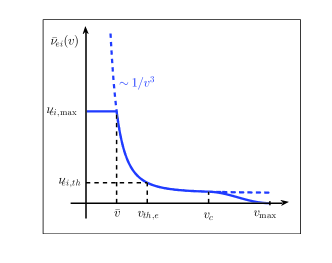
Figure 9: Modified electron-ion collision frequency as a function of velocity amplitude $v$.

Replacing the collision frequency $\nu_{\rm ei}(v)$ by $\bar{\nu}_{ei}(v)$, a good estimate based on Eq. (13 for the maximum eigenvalue of the discretized collision operator presented in Sec. A.2 is

$$\frac{\lambda_{\max}}{\nu_{\rm ei,th}}\simeq\pi^{2}\frac{v_{\rm th\,e}^{3}}{\Delta v^{2}}\frac{1}{\max(\Delta v,\bar{v})},$$ (56)

where $\Delta v$ is the velocity grid resolution. In case of unequal mesh spacings $\Delta v_{x}$ and $\Delta v_{y}$ in the $v_{x}$- and $v_{y}$- directions respectively, one sets $\Delta v=\min(\Delta v_{x},\Delta v_{y})$. Inserting Eq. (56) into relation (53) leads to the following estimate on the time constraint with respect to the collisional dynamics:

$$\Delta t\,\nu_{\rm ei,th}\lesssim\frac{\alpha}{\pi^{2}}\left(\frac{\Delta v}{v_{\rm th\,e}}\right)^{2}\frac{\max(\Delta v,\bar{v})}{v_{\rm th\,e}}.$$ (57)

How the modified collision frequency profile $\bar{\nu}_{\rm ei}(v)$, and in particular the capping at $\nu_{\rm ei,\max}$ of the maximum rate, affects physical results is addressed in Figure 10, where the dependence of the damping rate $\nu$ of an EPW on $\nu_{\rm ei,\max}$ is shown. The wavenumber considered is $k\lambda_{De}=0.3$ and the thermal collision rate $\nu_{ei,th}=1\cdot 10^{-1}\,\omega_{pe}$. According to the results in Fig. 10, a cap set as low as $\nu_{ei,\max}=10\,\nu_{ei,th}$, corresponding to $\bar{v}/v_{\rm th\,e}=10^{-1/3}\simeq 0.464$, has no discernable effect on the EPW damping rate.

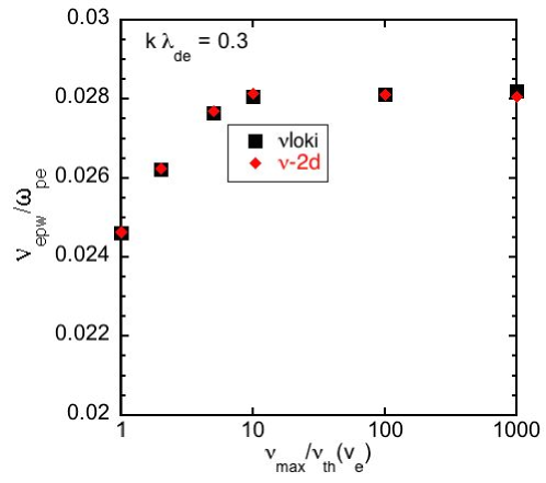
Figure 10: The dependence of the damping rate of an EPW with $k\lambda_{De}=0.3$ and $\nu_{ei,th}=0.1\omega_{pe}$ on the magnitude $\nu_{ei,\max}$ of the cap on $\nu_{ei}$. The results of both the LOKI simulations and the numerical solution to the 2D linearized set of equations are shown, both with the same cap. There is no effect discernable of the cap for $\nu_{max}/\nu_{ei,th}>10$.

Appendix B Recovering the Collisional Damping of EPWs from the Linearized Kinetic Models

The collisional damping of EPWs, already derived in the frame of a fluid description in Sec. III.3, is recovered here starting from the linearized Vlasov-Poisson systems presented in Sec. III.1. The cases of electron-ion pitch angle scattering in three- and two-dimensional velocity space are considered in turn in the following sections.

B.1 Collisional Damping of EPWs in Case of 3D Velocity Scattering

Consider equations (18) and (19) for the evolution of the first two coefficients $\delta f_{0}(v)$ and $\delta f_{1}(v)$ of the fluctuating part of the electron distribution decomposed in Legendre polynomials. For plane wave fluctuations with frequency $\omega$ and wavenumber $k$, these two equations read:

$$-i\omega\,\delta f_{0}+\frac{ikv}{3}\delta f_{1}=0,$$ (58)

$$-i\omega\,\delta f_{1}+ikv\,(\delta f_{0}-\phi\,f_{M})=-2\,\nu_{\rm ei}(v)\,\delta f_{1},$$ (59)

having neglected the coupling of $\delta f_{1}$ to $\delta f_{2}$ in Eq. (59). This approximation is justified in the collisonal limit, $k\lambda_{\rm ei}\ll 1$, as the ratio of consecutive coefficients scales as $|\delta f_{l+1}/\delta f_{l}|\sim k\lambda_{\rm ei}$. Equations for the higher order coefficients $\delta f_{l}$, $l\leq 2$, can thus be neglected. The set of equations (58) and (59) are identical to the ones considered in the diffusive approximation of Sec. III.5, except for the finite inertia term $\partial\,\delta\!f_{1}/\partial t\sim-i\omega\,\delta f_{1}$, which is clearly essential for modeling EPW dynamics.

From the set of Eqs. (58) and (59), $\delta f_{1}$ is eliminated to obtain the following expression for $\delta f_{0}$:

$$\delta f_{0}(v)=-\frac{(kv)^{2}f_{M}\,\phi}{3\omega\,[\omega+2i\nu_{\rm ei}(v)]-(kv)^{2}},$$

which is then inserted into the Poisson Eq. (21) to obtain the following dispersion relation:

$$\epsilon^{3D}(k,\omega)=1+\chi_{e}^{3D}(k,\omega)=0,$$ (60)

where the contribution $\chi_{e}^{3D}$ (corresponding to the electric susceptibility of electrons ) to the dielectric function $\epsilon^{3D}$ reads:

$$\chi_{e}^{3D}(k,\omega)=-\frac{1}{3}\sqrt{\frac{2}{\pi}}\int_{0}^{\infty}dv\frac{v^{4}\exp(-v^{2}/2)}{\omega^{2}+2i\omega\nu_{ei}(v)-k^{2}v^{2}/3}.$$ (61)

Assuming $\nu_{ei,th}\ll\omega_{pe}$, which together with the limit $k\lambda_{\rm ei}\ll 1$ also implies $k\lambda_{De}\ll 1$, the resonant denominator in this last relation can be Taylor expanded as follows to first order in these small terms:

$$\frac{1}{\omega^{2}+2i\omega\nu_{ei}(v)-k^{2}v^{2}/3}\simeq\frac{1}{\omega^{2}}\left[1+\frac{(kv)^{2}}{3\omega^{2}}-2i\frac{\nu_{ei}(v)}{\omega}\right],$$

providing, after having carried out the integral over velocity [here in unnormalized variables and using the relation $\nu_{ei}^{\rm brag}/\nu_{ei,th}=4/(3\sqrt{2\pi})$]:

$$\chi_{e}^{3D}=-\frac{\omega_{pe}^{2}}{\omega^{2}}\left(1+\frac{5}{3}\frac{(kv_{\rm th\,e})^{2}}{\omega^{2}}-i\frac{\nu_{ei}^{brag}}{\omega}\right).$$

Using this last relation, we obtain the following solution to the dispersion relation (60) in the limit $k\lambda_{De}\ll 1$ and $\nu_{ei,th}\ll\omega_{pe}$:

$$\omega=\omega_{R}-i\nu,\quad\text{with}\quad\omega_{R}=\omega_{pe}\sqrt{1+(5/3)(k\lambda_{De})^{2}}\quad\text{and}\quad\nu=\frac{\omega_{pe}}{\omega_{R}}\frac{\nu_{ei}^{\rm brag}}{2}\simeq\frac{\nu_{ei}^{\rm brag}}{2},$$

in full agreement with the dispersion relation (37) and collisional damping relation (38) derived in Sec. III.3, given the relation $\gamma_{e}=(d+2)/d=5/3$ for $d=D=3$. If the thermal corrections to the dispersion are kept, a $k\lambda_{De}$ dependence to the collisional damping is obtained.

Because $\nu_{ei}(v)\propto v^{-3}$, this Taylor expansion overemphasizes the contribution of low velocities whereas the largest contribution to the real and imaginary part of the integral in Eq. (61) comes from velocities $\sim v_{\rm th\,e}$. In fact, the Taylor expansion to the next order leads to a divergent integral. A numerical solution to the dispersion Eq. (60) for the damping rate is shown in Fig. 11 in the limit $k\lambda_{ei}\to 0$ and is about 1/2 the rate in Eq. (38) derived in Sec. III.3. Again, if the thermal corrections to the dispersion are retained, a $k\lambda_{De}$ dependence to the collisional damping is obtained. A similar dependence is shown in Fig. 4.

Figure 11: The collisional damping of EPWs is shown as obtained from LOKI simulations, the linearized Fokker-Planck equations, and from fluid equations. The solid blue and red lines are the numerical solutions for the collisional damping rate for Eq. (60) and Eq. (62) respectively in the limit that $k\lambda_{ei}\to 0$. The LOKI results for $k\lambda_{De}=0.2$ are shown by the black squares. The red diamonds are the same as shown in Fig. 5. They fall on the solid red line as they should because they are solving the same system of equations. The dashed red and blue lines are the damping rates from Eq. (38) obtained from the 2D and 3D fluid equations respectively. Note the fluid damping rates are larger than the simulation values and, contrary to the linearized Fokker-Planck results, larger in 2D than 3D.

B.2 Collisional Damping of EPWs in Case of 2D Velocity Scattering

We proceed as in Sec. B.1, but start from the first two equations (25) and (26) for the evolution of the first two coefficients $\delta f_{c,0}(v)$ and $\delta f_{c,1}(v)$ of the fluctuating part of the electron distribution decomposed in polar Fourier modes. Further making use of the Poisson equation (30), we obtain the following dispersion relation valid in the collisional limit $k\lambda_{\rm ei}\ll 1$:

$$\epsilon^{2D}(k,\omega)=1+\chi_{e}^{2D}(k,\omega)=0,$$ (62)

$$\chi_{e}^{2D}=-\frac{1}{2}\int_{0}^{\infty}dv\frac{v^{3}\exp(-v^{2}/2)}{\omega^{2}+i\omega\nu_{\rm ei}-k^{2}v^{2}/2}.$$ (63)

After Taylor expansion of the resonant denominator, the electric susceptibility is given by (in unnormalized variables):

$$\chi_{e}^{2D}=-\frac{\omega_{pe}^{2}}{\omega^{2}}\left(1+2\frac{(kv_{\rm th\,e})^{2}}{\omega^{2}}-i\sqrt{\frac{\pi}{8}}\frac{\nu_{ei,th}}{\omega}\right),$$

Using this last relation, we obtain the following solution to the dispersion relation (62) in the limit $k\lambda_{De}\ll 1$ and $\nu_{ei,th}\ll\omega_{pe}$:

$$\omega=\omega_{R}-i\nu,\quad\text{with}\quad\omega_{R}=\omega_{pe}\sqrt{1+2(k\lambda_{De})^{2}}\quad\text{and}\quad\nu=\frac{\omega_{pe}}{\omega_{R}}\sqrt{\frac{\pi}{2}}\frac{\nu_{ei,th}}{4}\simeq\sqrt{\frac{\pi}{2}}\frac{\nu_{ei,th}}{4},$$ (64)

in full agreement with the dispersion relation (37) and collisional damping relation (38) derived in Sec. III.3, where $\gamma_{e}=(d+2)/d=2$ for $d=D=2$. If the thermal corrections to the dispersion are kept, a $k\lambda_{De}$ dependence to the collisional damping is obtained. The damping rate in Eq. (64) is about twice larger than shown in Fig. 4 for the reasons explained in Sec.B.1 for the solution of the 3D dispersion (60). The numerical solution to the 2D dispersion Eq. (62) and the 3D dispersion Eq. (60 ) are shown in Fig. 11 along with the deduced LOKI collisional damping rates (also shown in Fig. 4) and the numerical solution to Eqs. (25) and (39) (also shown in Fig. 5). Note the 3D damping rate is larger than the 2D rate as expected from the kinetic results in Sec. III.2.

References

- Takizuka and Abe (1977) Takizuka and Abe, JCP 25, 205 (1977).
- Cohen et al. (2010) B. I. Cohen, A. M. Dimits, A. Friedman, and R. E. Calflisch, IEEE Trans. Plasma Sci. 38, 2394 (2010).
- Dimits et al. (2013) A. M. Dimits, B. I. Cohen, R. E. Calflisch, M. S. Rosin, and L. F. Ricketson, J. Comp. Phys. 242, 561 (2013).
- Cohen et al. (2006) B. I. Cohen, L. Divol, A. B. Langdon, and E. A. Williams, Phys. Plasmas 13, 022705 (2006).
- Kemp et al. (2010) A. J. Kemp, B. I. Cohen, and L. Divol, Phys. Plasmas 17, 056702 (2010).
- Ross et al. (2013) J. S. Ross, H.-S. Park, R. Berger, L. Divol, N. L. Kugland, W. Rozmus, D. Ryutov, and S. H. Glenzer, Phys. Rev. Lett. 110, 145005 (2013).
- Banks et al. (2011a) J. W. Banks, R. L. Berger, S. Brunner, B. I. Cohen, and J. A. F. Hittinger, Phys. Plasmas 18, 052102 (2011a).
- Winjum et al. (2013) B. Winjum, R. L. Berger, T. Chapman, J. W. Banks, and S. Brunner, Phy. Rev. Lett. 111, 115002 (2013).
- Berger et al. (2015) R. L. Berger, S. Brunner, J. W. Banks, B. I. Cohen, and B. J. Winjum, Phys. Plasmas 22, 055703 (2015).
- Epperlein (1994) E. M. Epperlein, Laser Part. Beams 12, 257 (1994).
- Brunner and Valeo (2002) S. Brunner and E. J. Valeo, Phys. Plasmas 9, 923 (2002).
- Tzoufras et al. (2011) M. Tzoufras, A. R. Bell, P. A. Norreys, and F. S. Tsung, J. Comput. Phys. 230, 6475 (2011).
- Braginskii (1965) S. I. Braginskii, Particle Interactions in a Fully Ionized Plasma (M. A. Leontovich, Consultants Bureau, New York, 1965), vol. 1 of Reviews of Plasma Physics, p. 205.
- Albritton et al. (1986) J. R. Albritton, E. A. Williams, I. B. Bernstein, and K. P. Swartz, Phys. Rev. Lett. 57, 1887 (1986).
- Epperlein and Short (1991) E. M. Epperlein and R. W. Short, Phys. Fluids B 3, 3092 (1991).
- Bychenkov et al. (1995) V. Y. Bychenkov, W. Rozmus, and V. Tikhonchuk, Phys. Rev. Lett. 75, 4405 (1995).
- Brantov et al. (1996) A. V. Brantov, V. Y. Bychenkov, and V. Tikhonchuk, JETP 83, 716 (1996).
- Schurtz et al. (2000) G. P. Schurtz, P. D. Nicolai, and M. Busquet, Phys. Plasmas 7, 4238 (2000).
- Brantov et al. (2012) A. V. Brantov, V. Y. Bychenkov, and W. Rozmus, Phys. Rev. Lett. 108, 205001 (2012).
- Epperlein et al. (1992) E. M. Epperlein, R. W. Short, and A. Simon, Phys. Rev. Lett. 69, 1765 (1992).
- Berger and Valeo (2005) R. L. Berger and E. J. Valeo, Phys. Plasmas 12, 032104 (2005).
- Brunner et al. (2014) S. Brunner, R. L. Berger, B. I. Cohen, L. Hausammann, and E. J. Valeo, Phys. Plasmas 21, 102104 (2014).
- Berger et al. (2013) R. L. Berger, S. Brunner, T. Chapman, L. Divol, C. H. Still, and E. J. Valeo, Phys. Plasmas 20, 032107 (2013).
- Strozzi et al. (2012) D. J. Strozzi, E. A. Williams, H. A. Rose, D. E. Hinkel, A. B. Langdon, and J. W. Banks, Phys. Plasmas 19, 112306 (2012).
- Banks and Hittinger (2010) J. W. Banks and J. A. F. Hittinger, IEEE T. Plasma. Sci. 38, 2198 (2010).
- Banks et al. (2011b) J. W. Banks, R. L. Berger, S. Brunner, B. I. Cohen, and J. A. F. Hittinger, Phys. Plasmas 18, 052102 (2011b).
- Callen (2014) J. D. Callen, Phys. Plasmas 21, 052106 (2014).
- Su and Oberman (1968) C. H. Su and C. Oberman, Phys. Rev. Lett. 20, 427 (1968).
- Auerbach (1977) S. P. Auerbach, Phys. Fluids 20, 1836 (1977).
- Zheng and Qin (2013) J. Zheng and H. Qin, Phys. Plasmas 20, 092114 (2013).
- Brantov et al. (2004) A. V. Brantov, V. Y. Bychenkov, W. Rozmus, and C. E. Capjack, Phys. Rev. Lett. 93, 125002 (2004).
- Albritton (1983) J. R. Albritton, Phys. Rev. Lett. 50, 2078 (1983).
- Kampen (1955) N. G. V. Kampen, Physica 21, 949 (1955).
- O’Neil (1965) T. M. O’Neil, Phys. Fluids 8, 2255 (1965).
- Morales and O’Neil (1972) G. J. Morales and T. O’Neil, Phy. Rev. Lett. 28, 417 (1972).
- Bernstein et al. (1957) I. B. Bernstein, J. M. Greene, and M. D. Kruskal, Phys. Review 108, 546 (1957).
- Brunner (2009) S. Brunner, Tech. Rep., LLNL (2009).
- Gould et al. (1967) R. W. Gould, T. M. O’Neil, and J. H. Malmberg, Phys. Rev. Lett. 19, 219 (1967).
- Malmberg et al. (1968) J. H. Malmberg, C. B. Wharton, R. W. Gould, and T. M. O’Neil, Phys. Fluids. 11, 1147 (1968).
- Baker et al. (1968) D. R. Baker, N. R. Ahearn, and A. Y. Wong, Phys. Rev. Lett. 20, 318 (1968).
- Henshaw (2006) W. D. Henshaw, SIAM J. Sci. Comput. 28, 1730 (2006).
- Fornberg (1996) B. Fornberg, A Practical Guide to Pseudospectral Methods (Cambridge University Press, Cambridge, 1996).