Multiple mobility edges in a 1D Aubry chain with Hubbard interaction in presence of electric field: Controlled electron transport

Abstract

Electronic behavior of a 1D Aubry chain with Hubbard interaction is critically analyzed in presence of electric field. Multiple energy bands are generated as a result of Hubbard correlation and Aubry potential, and, within these bands localized states are developed under the application of electric field. Within a tight-binding framework we compute electronic transmission probability and average density of states using Green’s function approach where the interaction parameter is treated under Hartree-Fock mean field scheme. From our analysis we find that selective transmission can be obtained by tuning injecting electron energy, and thus, the present model can be utilized as a controlled switching device.

I Introduction

Electron transport in low-dimensional system has created a lot of interest among researchers due to its immense applicability in the field of nanoscience. Transport in low-dimensional systems led to interesting quantum effects. In one-dimension ($1$D) in presence of random disorder all the eigenstates are exponentially localized irrespective of however weak is the strength of disorder, this is the well-known phenomenon of Anderson localization ander . Based on this fact it is a common belief that no mobility edge, energy eigenvalues separating localized states from the extended states, can exist in 1D. In addition to Anderson localization there exists another kind of localization which is Wannier Stark localization wann that occurs due to application of bias voltage. It has also drawn much attention like the case of Anderson localization. Here localization is obtained even in absence of disorder and only due to the resulting electric field. Many theoretical wt1 ; wt2 ; wt3 ; wt4 ; wt5 and experimental wae analysis are available on Stark localization just like Anderson localization. Even in this case mobility edge could not be detected.

However, it has been pointed out that in correlated disordered systems all eigenstates are not localized angel , rather some states are of extended in nature as well. In a work Dunlap et al. considered a random dimer model dunlap and showed that the system supports extended eigenstates at certain discrete eigenvalues. Similarly, a number of works have also appeared in the literature l1 ; l2 ; ssa2 ; sn1 to establish the presence of delocalized states along with the localized ones thereby exhibiting metal to insulator transition. With all these special classes of lattice models, Aubry-Andre (AA) model abam always gives a a classic signature in transport phenomena. The on-site potential in the AA 1D chain has the form of a cosine function mag ; sharma ; eco :

$$\epsilon_{n}=\lambda\cos(Qna)$$ (1)

where $\lambda$ is the modulation amplitude, $Q$ is an irrational multiple of $\pi$ and $a$ is the lattice spacing. It is a quasiperiodic lattice something intermediate between periodic and random disordered systems. The parameter $\lambda$ has an important role on the localization behavior of the eigenstates. Using Thouless formula thf Aubry and Andre demonstrated that this model exhibits energy independent metal insulator transition in the parameter space of the Hamiltonian at $\lambda=2t$, where $t$ represents the nearest-neighbor hopping integral. For $\lambda<2t$ all eigenstates are extended and in case of $\lambda>2t$ all are localized, the equality relation is the point of duality with exotic critical eigenstates which are neither extended nor localized. This interesting feature of the AA model aroused immense

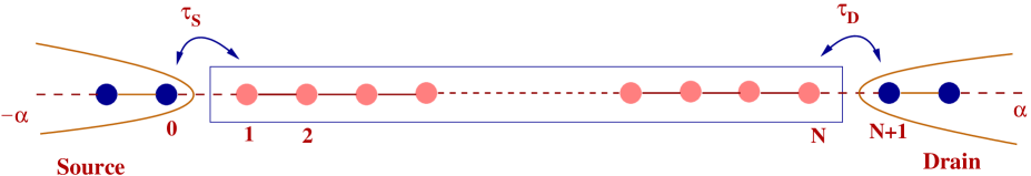
Figure 1: (Color online). Schematic diagram of a $1$D tight-binding chain coupled to two $1$D semi-infinite electrodes, viz, source and drain.

curiosity in the minds of researchers to advance in this field. Large number of articles dealt with this model both for $1D$ chain as well as in case of ladder aubry79 ; ssa1 . However to the best of our knowledge, the study of the phenomenon of Stark localization in an AA chain in presence of Hubbard interaction is absent in literature. In the present manuscript we have elaborately studied the phenomena of localization in a 1D AA chain in absence and presence of electron-electron (e-e) interaction. First we analyze the effect of applied bias voltage on the localization behavior of AA chain in absence of any Hubbard interaction and finally we approach to the case in presence of interaction. Thus we see how an interesting interplay of localization as well as mobility edge phenomena occurring.

Rest of the article is arranged as follows. In Section II we present the model and theory based on which the results have been derived and discussed in Section III. Lastly we conclude in Section IV.

II Model and Theory

Figure 1 depicts a one-dimensional AA chain coupled to two semi-infinite leads. The chain comprising $N$ atomic sites is subjected to an incommensurate Aubry potential. We describe the model embracing the tight-binding formalism and Hamiltonian for the entire system can be expressed as,

$$H=H_{S}+H_{chain}+H_{tun}+H_{D}$$ (2)

where the different sub-Hamiltonians are described as follows. The Hamiltonians

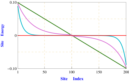
Figure 2: (Color online). Variation of voltage dependent on-site potentials in a $1$D chain with $200$ atomic sites when the bias voltage is fixed at $0.2\,$V. Three different electrostatic potential profiles, one linear and two non-linear, are taken into account those are represented by three different colored curves.

for the semi-infinite source and drain electrodes are $H_{S(D)}$ and they can be written explicitly as,

$$H_{S(D)}=\sum\limits_{p}\epsilon_{0}d_{p}^{{\dagger}}d_{p}+\sum\limits_{p}t_{0}[d_{p+1}^{{\dagger}}d_{p}+h.c.]$$ (3)

where $\epsilon_{0}$ and $t_{0}$ correspond to the on-site energy and nearest-neighbor hopping integral, respectively, in the electrodes. Creation and annihilation operators of electron inside the electrodes in the $n$th Wannier state are respectively denoted by $d_{n}^{{\dagger}}$ and $d_{n}$.

The second term in Eq. 2 describes the Hamiltonian for the 1D AA chain. In absence of electron-electron interaction, the AA chain has on-site energy of the form $\epsilon_{i}=\lambda\cos(Qia)$ where, $a$ represent the lattice constant, $Q$ is an irrational multiple of $\pi$ and $i$ corresponds to positions of atomic sites. Therefore Hamiltonian for a non-interacting AA chain is of the form

$$H_{chain}=\sum\limits_{i}\epsilon_{i}c_{i}^{{\dagger}}c_{i}+\sum\limits_{i}t[c_{i+1}^{{\dagger}}c_{i}+h.c.]$$ (4)

$t$ being nearest-neighbor hopping integral and $c_{i}^{{\dagger}}$ ($c_{i}$ ) denotes the creation (annihilation) operator in the AA chain. When all site energies are identical, the AA chain maps to a perfect ordered chain and in that case we set $\epsilon_{i}=0$ $\forall\;i$, without loss of generality. As we apply bias voltage $V$ across the chain, it results an electric field to develop across it and the on-site energy gets modified to $\epsilon_{i}^{\prime}=\epsilon_{i}+\epsilon_{i}(V)$, where $\epsilon_{i}(V)$ is the voltage dependent part of on-site energy. Now, the question naturally comes how on-site energy depends on the voltage. Several attempts pr1 ; pr2 ; pr3 ; pr4 ; pr5 ; pr6 have been done along this line to find potential profile along a linear conductor coupled to source and drain electrodes. Mostly ab initio or semiempirical models are used, but few groups have also done it by solving Poisson’s equations. From these studies it has been suggested that depending on electron screening, potential profile along a conductor sandwiched between source and drain can be of linear type or non-linear one. For very large screening length linear voltage drop is expected, while entire voltage drops at the interfaces between chain and electrode for very short screening length pr5 . Considering symmetric potential drop at the two interfaces we can write voltage dependent on-site energy for linear potential profile as pr7 $\epsilon_{i}(V)$=$V/2-iV/(N+1)$, where $V$ is the applied bias voltage. While, for non-linear potential profile there is no such specific functional form. Keeping in mind the effect of electron screening, in our model calculations we choose two different functional forms for two non-linear curves as shown in Fig. 2. For pink curve we set $V/2\;\mbox{Exp}[-iV/5]$, while for blue curve it gets the form $V/2\;\mbox{Exp}[-iV/1.5]$. Running the variable $i$ (viz, site index) from $1$ to $N/2$ we generate the datas for fixed voltage $V$ and then for $N/2+1$ to $N$ values of $i$ we take the negative of these values in reverse order to make the profile symmetric. One can also take other functional forms to generate these identical curves and the entire physics will remain same as electron transport depends only on the values of voltage dependent on-site energies, not on the actual functional form. Here two non-linear profiles correspond to two different electron screening as suggested by earlier studies pr5 ; pr6 . Here it is important to note that, the variation of electrostatic potential profile depends on the material itself. But for our model calculations we consider these three different profiles, and, we believe that with our results general features of electric field on electron transmission across a junction can be clearly analyzed.

The third term represents coupling Hamiltonian due to the coupling of the AA chain and side-attached leads, and it reads as

$$H_{tunn}=\tau_{S}[c_{1}^{\dagger}d_{0}+h.c.]+\tau_{D}[c_{N}^{\dagger}d_{N+1}+h.c.]$$ (5)

where $\tau_{S}$ and $\tau_{D}$ give the strengths by which the system is coupled to source and drain, respectively.

Now if we incorporate on-site Coulomb interaction in the AA chain through Hubbard term along with the effect of bias voltage, the Hamiltonian takes the form,

$$H_{chain} = \sum\limits_{i,\sigma}\epsilon_{i,\sigma}^{\prime}c_{i,\sigma}^{\dagger}c_{i,\sigma}+\sum\limits_{\langle ij\rangle,\sigma}t[c_{i,\sigma}^{\dagger}c_{j,\sigma}+c_{j,\sigma}^{\dagger}c_{i,\sigma}]$$ (6)

$$+ \sum\limits_{i}Uc_{i\uparrow}^{\dagger}c_{i\uparrow}c_{i\downarrow}^{\dagger}c_{i\downarrow}$$

where $U$ is the Coulomb interaction strength.

To study electronic behavior of such an interacting system we use Hartree-Fock mean field kato ; kam ; new1 theory. In this approach, Eq. 6 can be written as

$$H_{chain} = \sum_{i}\epsilon_{i\uparrow}^{\prime\prime}n_{i\uparrow}+\sum_{\langle ij\rangle}t\left[c_{i\uparrow}^{\dagger}c_{j\uparrow}+c_{j\uparrow}^{\dagger}c_{i\uparrow}\right]$$ (7)

$$+ \sum_{i}\epsilon_{i\downarrow}^{\prime\prime}n_{i\downarrow}+\sum_{\langle ij\rangle}t\left[c_{i\downarrow}^{\dagger}c_{j\downarrow}+c_{j\downarrow}^{\dagger}c_{i\downarrow}\right]$$

$$- \sum_{i}U_{i}\langle n_{i\uparrow}\rangle\langle n_{i\downarrow}\rangle$$

$$= H_{c,\uparrow}+H_{c,\downarrow}-\sum_{i}U_{i}\langle n_{i\uparrow}\rangle\langle n_{i\downarrow}\rangle$$

where, $H_{c,\uparrow}$ and $H_{c,\downarrow}$ are Hamiltonians for the up and down spin electrons, respectively, similar to Eq. 4 with modified on-site energies as $\epsilon_{i,\uparrow}^{\prime\prime}=\lambda\cos(Qia)+\epsilon_{i}(V)+U\langle n_{i,\downarrow}\rangle$ and $\epsilon_{i,\downarrow}^{\prime\prime}=\lambda\cos(Qia)+\epsilon_{i}(V)+U\langle n_{i,\uparrow}\rangle$, $n_{i,\sigma}=c_{i,\sigma}^{\dagger}c_{i,\sigma}$ being the number operator. The last term in the above equation (Eq. 7) represents a shift in the total energy and it depends on the average number of up and down spin electrons. Once we get the decoupled Hamiltonians for up and down spin electrons, we find the eigenvalues self-consistently considering some initial guess values of $\langle n_{i,\uparrow}\rangle$ and $\langle n_{i,\downarrow}\rangle$. With the starting guess values of $\langle n_{i,\sigma}\rangle$ we diagonalize the Hamiltonians $H_{c,\uparrow}$ and $H_{c,\downarrow}$, and compute a new set of values for $\langle n_{i,\sigma}\rangle$. Next we replace the initial guess values with the new set of values of $\langle n_{i,\sigma}\rangle$ and repeat the process until the values of all $\langle n_{i,\sigma}\rangle$ converges. Substituting the final set of values in the Hamiltonians we calculate the two-terminal transmission probability using the Landauer formula. Transmission probability for up or down spin evaluated separately in terms of Green’s function from the relation datta1

$$T_{\sigma}(E)=Tr[\Gamma_{S}^{\sigma}G_{chain,\sigma}^{r}\Gamma_{D}^{\sigma}G_{chain,\sigma}^{a}]$$ (8)

where $\Gamma_{S(D)}^{\sigma}$ is the coupling matrix bearing the imaginary part of the self-energy $\Sigma_{S(D)}^{\sigma}$, arising due to the coupling between chain and the semi-infinite leads. $G_{chain,\sigma}^{r}$ and $G_{chain,\sigma}^{a}$ are the retarded and advanced Green’s functions of the chain which include the effect of electrodes. Thus we can write datta1 $G_{chain,\sigma}^{r}=(E-H_{c,\sigma}-\Sigma_{S}^{\sigma}-\Sigma_{D}^{\sigma})^{-1}$. For complete derivation of self-energies and effective Green’s function ($G_{chain,\sigma}$) of the chain, see Appendix A and Ref. datta1 . Determining transmission probabilities of up and down spin electrons we can calculate the total transmission probability from the relation $T(E)=\sum\limits_{\sigma}T_{\sigma}(E)$. Finally, we evaluate the average density of states (ADOS) using the relation $\rho(E)=-(1/N\pi)Tr[Im[G_{chain}^{r}]]$.

During the computation we use $\lambda=1$ in unit of $t$ (eV), except for Fig. 5 where $\lambda$ is varying, and set $Q=(1+\sqrt{5})/2$. The other common parameters are as follows: $\tau_{S}=\tau_{D}=1\;$eV, $t=1\;$eV, $\epsilon_{0}=0$ and $t_{0}=2\;$eV. The on-site energy ($\epsilon_{i,\uparrow}^{\prime\prime}$ or $\epsilon_{i,\downarrow}^{\prime\prime}$) in the chain, a sum of tree terms ($\lambda\cos(Qia)$, $\epsilon_{i}(V)$ and $U\langle n_{i,\downarrow}\rangle$ or $U\langle n_{i,\uparrow}\rangle$), on the other hand is not a constant, and therefore, we cannot assign a common value of it. Throughout the calculations we measure all energies in unit of $t$ and bias voltage in unit of Volt ($V$) and set $c=e=h=1$, for simplification.

III Numerical Results and Discussion

In this section we present the results based on the above theoretical formulation.

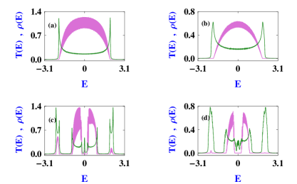
Figure 3: (Color online). Total transmission probability (pink color) and average DOS (green color) vs. energy $E$ for a non-interacting chain considering $N=200$ and $U=0$, where (a) and (b) correspond to the chain with identical site potentials, while (c) and (d) represent the Aubry chain. For the left column we set $V=0$, and, it is $0.2$ for the right column. The results are computed for the linear bias drop across the chain.

First we study the case of electron transmission through a non-interacting AA chain in presence of bias voltage and then we consider effect of Hubbard interaction into it.

Figures 3(a) and (b) present the results for the case of a non-interacting 1D chain in absence of incommensurate potential i.e., the chain becomes a perfect $1$D lattice. For such a case we choose the bare site potentials to zero, without loss of generality. In Fig. 3(a) we set the bias voltage $V$ to zero, while it is fixed at $0.2$ in Fig. 3(b). In absence of external bias voltage all the energy eigenstates are extended in nature, and therefore, the transmission probability is finite at all

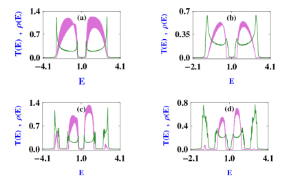
Figure 4: (Color online). Total transmission probability and average DOS as a function of energy $E$ for an interacting chain with $U=2$, where (a)-(d) correspond to the identical meaning as in Fig. 3. All the other parameters are same as considered in Fig. 3.

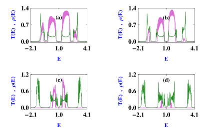
Figure 5: (Color online). $T$-$E$ and $\rho(E)$-$E$ curves for a $200$ site interacting chain ($U=2$) for different values of $\lambda$, where (a), (b), (c) and (d) correspond to $\lambda=0.5$, $1$, $2$ and $2.5$, respectively. For all these cases we set $V=0$.

energy eigenvalues. In presence of finite bias eigenstates at the band edges are no longer extended as it is evident from Fig. 3(b) that the transmission probability is zero while inside the band eigenstates are extended as we have finite transmission probability. It indicates that the choice of Fermi energy is quite important. If it is chosen to lie well inside the energy band the chain will be of conducting nature, while if it lies near the band edges the chain behaves as an insulator. Such sharp transitions of the conducting behavior gives an idea of existence of mobility edges in presence of a finite bias. In the same figure, cases (c) and (d) represent the transmission probability and ADOS of a non-interacting AA chain in absence and presence of a linear bias drop. Presence of incommensurate potential leads to splitting of band. We see that there are two gaps embedded inside three bands. In presence of bias voltage, say $V=0.2$, the energy eigenstates belonging to the outermost two bands have negligible contribution to transmission unlike those of the middle band, and hence extended energy eigenstates as well as the localized ones are present leading to metal-insulator transition. The more we increase the bias voltage, more number of localized states will appear and at one stage all the states will be localized.

Next we study the interplay between electric field and the Aubry ordering in 1D Hubbard chain. The transmission characteristics together with ADOS

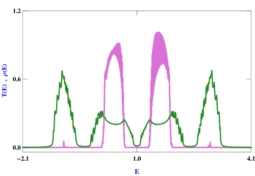
Figure 6: (Color online). $T$-$E$ and $\rho(E)$-$E$ characteristics for an interacting AA chain considering $300$ atomic sites with $U=2$ and $\lambda=1$. The results are shown for a linear bias drop when $V=0.3$.

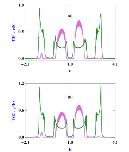
Figure 7: (Color online). $T$-$E$ and $\rho(E)$-$E$ characteristics for an interacting AA chain with $N=200$, $U=2$ and $\lambda=1$ considering non-linear bias drop across the chain. In (a) set the electrostatic potential profile as given by the pink line in Fig. 2, while in (b) we choose it according to the blue line of Fig. 2. Here we fix $V=0.2$.

of an AA interacting chain are shown in Fig. 4. First row represents $T(E)$ and $\rho(E)$ as functions of $E$ for an interacting chain in absence of Aubry potential. In the half-filled case we have a Mott insulator (Fig. 4(a)) with a single gap at the band centre. For the $1$D AA Hubbard chain, we have a Mott gap at the center of the band, but additional gaps appear due to Aubry potential as clearly seen from Fig. 4(c). In absence of bias voltage, all the eigenstates of the periodic as well as the AA Hubbard chains have finite electron transmission probability. On the other hand, in presence of finite bias localized states appear at the band edges both in case of a $1$D periodic Hubbard chain (Fig. 4(b)) and $1$D AA Hubbard chain (Fig. 4(d)).

To investigate the precise role of $\lambda$ on transmission and ADOS we present results for different values of $\lambda$ in Fig. 5 setting $V=0$. We see that for $\lambda<2t$, all the eigenstates are of extended in nature even in presence of $U$. The fact that for $\lambda<2t$ all the eigenstates of $1$D AA chain behave like extended states and their behavior remains unaltered even for $U\neq 0$ which can be noticed from Figs. 5(a) and (b). It is well known that for $\lambda=2t$ states are critical and for $\lambda>2t$ all the eigenstates are localized, and for both these cases we have zero transmission probability. Quite interestingly from Figs. 5(c) and (d) we see that few conducting states appear in the middle of the inner two bands when $U\neq 0$. Physically it implies that electron-electron interaction changes the behavior of the AA chain.

To test the invariant nature of the above discussed phenomena with respect to the parameter values, in Fig. 6 we present the characteristics features of transmission probability together with average density of states considering a chain with different set of parameter values where $N=300$ and $V=0.3$. From the spectra it is clear that all the physical pictures remain unchanged and certainly it strengthens the invariant character of our analysis and can be verified experimentally.

Till now we have shown all the cases in presence of linear voltage drop across the chain. To get an idea regarding the behavior of transmission and average density of states in presence of non-linear bias drop let us focus on the results given in Fig. 7. Two different non-linear profiles are taken into account following the curves (pink and blue lines) shown in Fig. 2. For these two cases we also get similar kind of band splitting and localization phenomenon, but a careful observation suggests that the transmission probability becomes higher for the flatter profile (blue line of Fig. 2) compared to the other (pink line of Fig. 2) one. With increasing the flatness the localization effect due to electric field decreases, and, for the limiting case i.e., when the bias drop takes place only at the two edges of the chain, transmission probability will be maximum when all the other parameters are kept unchanged.

IV Conclusion

In the present work we critically investigate the role of electric field, developed due to external bias, in an interacting $1$D Aubry chain. The interaction parameter is described within a Hartree-Fock mean field level under tight-binding framework where transmission probability and ADOS are evaluated from Green’s function approach. The interplay between Aubry lattice, Coulomb correlation and electric field provides multiple mobility edges at different energies. Under this situation if we scan throughout the energy band window then electrons can allow to pass from source to drain via the selective conducting energy channels providing finite electron transmission, while for all other cases we get the insulating phase since then no electron can transmit through the localized channels. This phenomenon clearly emphasizes that the present model can be utilized as a selective switching device.

Appendix A Evaluation of self-energies and effective Green’s function of the chain coupled to source and drain electrodes

Since there is no spin flip mechanism (viz, from up spin to down spin or vice versa) in our problem, the net transmission probability is obtained from the relation $T(E)=\sum_{\sigma}T_{\sigma}(E)=T_{\uparrow}+T_{\downarrow}$. To find $T_{\sigma}$ we need to evaluate $H_{c,\sigma}$, $\Sigma_{S}^{\sigma}$, $\Sigma_{D}^{\sigma}$ and the effective Green’s function $G_{chain,\sigma}$. The Hamiltonian $H_{c,\sigma}$ is determined from the mean field scheme which is clearly described in Sec. II, and therefore, here we discuss elaborately how to calculate other factors i.e., self energies and effective Green’s function. For this, we can now ignore the spin index, as a matter of simplification, because the prescription is same for both the two spin cases.

Following the definition we can write the Green’s function of the full system,

$$G^{r}=\left[(E+i\eta)I-H\right]^{-1}.$$ (9)

where, $I$ is the identity matrix and $\eta\rightarrow 0^{+}$. But there is a problem with Eq. 9. Here we are working with an open system i.e., a conductor connected with two semi-infinite electrodes. Therefore, $H$ has infinite dimension and so also $G^{r}$. Now it is not possible to do any calculation with a matrix whose dimension is infinity. So, to get rid of this situation we apply the partitioning technique which maps the Green’s function matrix in the reduced Hilbert space of the conductor itself, and the effects of the side attached leads are incorporated there.

Suppose we are considering a conductor attached to electrode $p$. Hence, the total Hamiltonian of the system can be written in a matrix form as,

$$H=\left(\begin{array}[]{cc}H_{p}&\tau_{p}\\ \tau_{p}^{\dagger}&H_{c}\end{array}\right).$$ (10)

Here, $H_{c}$ and $H_{p}$ are the Hamiltonian matrices describing the conductor and the side attached electrode. $\tau_{p}$ corresponds to the coupling matrix due to coupling of the conductor to the side attached electrode.

Hence, the Green’s function is,

$$G^{r} = \left((E+i\eta)I-H\right)^{-1}$$ (13)

$$= \left(\begin{array}[]{cc}(E+i\eta)I-H_{p}&-\tau_{p}\\ -\tau_{p}^{\dagger}&EI-H_{pc}\end{array}\right)^{-1}$$

Now, partitioning the Green’s function matrix in the same way like the Hamiltonian matrix, we can rewrite the above equation as,

$$\left(\begin{array}[]{cc}G_{p}&G_{pc}\\ G_{cp}&G_{c}\end{array}\right) = \left(\begin{array}[]{cc}(E+i\eta)I-H_{p}&-\tau_{p}\\ -\tau_{p}^{\dagger}&EI-H_{c}\end{array}\right)^{-1}$$ (18)

i.e.,

$$\left(\begin{array}[]{cc}G_{p}&G_{pc}\\ G_{cp}&G_{c}\end{array}\right)\left(\begin{array}[]{cc}(E+i\eta)I-H_{p}&-\tau_{p}\\ -\tau_{p}^{\dagger}&EI-H_{c}\end{array}\right) = \left(\begin{array}[]{cc}1&0\\ 0&1\end{array}\right)$$ (25)

We obtain two decoupled equations from the above equation, which are as follows,

$$G_{cp}\left[(E+i\eta)I-H_{p}\right]-G_{c}\tau_{p}^{\dagger}=0$$ (27)

and,

$$-G_{cp}\tau_{p}+G_{c}(EI-H_{c})=1$$ (28)

We define, $(E+i\eta)I-H_{p}=(g_{p}^{r})^{-1}$. So, from Eq. (27) we get,

$$G_{cp}(g_{p}^{r})^{-1} = G_{c}\tau_{p}^{\dagger}$$

$$\Rightarrow G_{cp} = G_{c}\tau_{p}^{\dagger}g_{p}^{r}$$ (29)

Using the expression of $G_{cp}$ from Eq. (29) in Eq. (28), we get,

$$-G_{c}\tau_{p}^{\dagger}g^{r}_{p}\tau_{p}+G_{c}(EI-H_{c})=1$$ (30)

$$\Rightarrow G_{c}\left[EI-H_{c}-\tau_{p}^{\dagger}g^{r}_{p}\tau_{p}\right]=1$$

$$\Rightarrow G_{c}\left[EI-H_{c}-\Sigma_{p}\right]=1$$

$$\Rightarrow G_{c}=\left[EI-H_{c}-\Sigma_{p}\right]^{-1}$$

where,

$$\Sigma_{p}=\tau_{p}^{\dagger}g^{r}_{p}\tau_{p}$$ (31)

Here, $G_{c}(=\mathcal{G})$ is the effective Green’s function which incorporates the effect of the electrode attached with the conductor.

In Eq. 30, all matrices have the same dimension ($C$ $\times$ $C$), where, $C$ is the dimension of the conductor. But at first sight it might appear that the problem of inverting an infinite dimensional matrix still remains, while evaluating $g^{r}_{p}$ to obtain the expression for $\Sigma_{p}$. But fortunately for an isolated infinite lead $g^{r}_{p}$ can be calculated analytically.

Now for $ij$-th element of the self-energy matrix,

$$\Sigma_{ij} = \langle i|\tau_{p}^{\dagger}g_{p}^{r}\tau_{p}|j\rangle$$ (32)

$$= \sum_{m,n}\langle i|\tau_{p}^{\dagger}|m\rangle\langle m|g_{p}^{r}|n\rangle\langle n|\tau_{p}|j\rangle$$

$$= t^{2}g_{p}^{r}(p_{i},p_{j}).$$

Here, $g_{p}^{r}(p_{i},p_{j})$ denotes the ($p_{i},p_{j}$)-th element of the matrix $g_{p}^{r}$. To work with Eq. 30 we have to reconstruct the $\Sigma_{p}$ matrix in $C$ $\times$ $C$ dimension. Here, all elements of $\Sigma_{p}$ matrix would be zero, except at the points ($i$,$j$) inside the conductor, which are adjacent to points ($p_{i}$,$p_{j}$) inside the electrode.

For more than one electrodes we have to add the effects of individual electrodes. It means if we have $p$ number of side-attached electrodes, then the effective Green’s function will be,

$$\mathcal{G}=[EI-H_{c}-\sum\limits_{p}\Sigma_{p}]^{-1}$$ (33)

From this expression we can easily write the desired effective Green’s function for our two-terminal system as $\mathcal{G}=G_{chain}=(E-H_{c}-\Sigma_{S}-\Sigma_{D})^{-1}$ which includes the effects of both source and drain electrodes. For two different spin sub-spaces it can be generalized as $G_{chain,\sigma}=(E-H_{c,\sigma}-\Sigma_{S}^{\sigma}-\Sigma_{D}^{\sigma})^{-1}$.

References

- (1) P. W. Anderson, Phys. Rev. 109, 1492 (1958).
- (2) G.H. Wannier, Phys. Rev. 117 432 (1960).
- (3) H. M. James, Phys. Rev. 76, 1611 (1949).
- (4) D. Emin and C. F. Hart, Phys. Rev. B 36, 7353 (1987).
- (5) R. Ouasti, N. Jekri, A. Brezini, and C. Depollier, J. Phys.: Condens. Matter. 7, 811 (1995).
- (6) N. Zekri, M. Schreiber, R. Ouasti, R. Bouamrane, and A. Brezini, Z. Phys. B 99, 381 (1996).
- (7) J. R. Borysowicz, Phys. Lett. A. 231, 240 (1997).
- (8) C. Hamaguchi, M. Yamaguchi, H. Nagasawa, M. Morifuji, A. Di Carlo, P. Vogl, G. Bohm, G. Trankle, G. Weimann, Y. Nishikawa and S. Muto, Jpn. J. Appl. Phys. 34, 4519 (1995).
- (9) A. Sanchez, Phys. Rev. B 49, 147 (1994).
- (10) D. H. Dunlap, H.-L. Wu, and P. Phillips, Phys. Rev. Lett. 65, 88 (1990).
- (11) X. F. Hu, Z. H. Peng, R. W. Peng, Y. M. Liu, F. Qiu, X. Q. Huang, A. Hu, and S. S. Jiang, J. Appl. Phys. 95, 7545 (2004).
- (12) R. L. Zhang, R. W. Peng, X. F. Hu, L. S. Cao, X. F. Zhang, M. Wang, A. Hu, and S. S. Jiang, J. Appl. Phys. 99, 08F710 (2006).
- (13) S. Sil, S. K. Maiti, and A. Chakrabarti, Phys. Rev. B 78, 113103 (2008).
- (14) S. K. Maiti and A. Nitzan, Phys. Lett. A 377, 1205 (2013).
- (15) S. Aubry and G. Andre, in: L. Horwitz, Y. Neeman (Eds.), Group Theoretical Methods in Physics, Annals of the Israel Physical Society, Vol. 3, American Institute of Physics, New York, 1980, p. 133.
- (16) M. Johansson and R. Riklund, Phys. Rev. B 42, 8244 (1990).
- (17) S. Das Sarma, S. He, and X.C. Xie, Phys. Rev. Lett. 61, 2144 (1988).
- (18) C. M. Soukoulis and E. N. Economou, Phys. Rev. Lett. 48, 1043 (1982).
- (19) D. J. Thouless, J. Phys. C 5, 77 (1972).
- (20) S. Aubry and G. Andre, Ann. Isr. Phys. Soc. 3, 133 (1979).
- (21) S. Sil, S. K. Maiti, and A. Chakrabarti, Phys. Rev. Lett. 101, 076803 (2008).
- (22) S. Datta, W. Tian, S. Hong, R. Reifenberger, J. I. Henderson, and C. P. Kubiak, Phys. Rev. Lett. 79, 2530 (1997).
- (23) W. Tian, S. Datta, S. Hong, R. Reifenberger, J. I. Henderson, and C. P. Kubiak, J. Chem. Phys. 109, 2874 (1998).
- (24) V. Mujika, A. E. Roitberg, and M. A. Ratner, J. Chem. Phys. 112, 6834 (2000).
- (25) N. D. Lang and P. Avouris, Phys. Rev. Lett. 84, 358 (2000).
- (26) A. Nitzan, M. Galperin, G.-L. Ingold, and H. Grabert, J. Chem. Phys. 117, 10837 (2002).
- (27) S. Pleutin, H. Grabert, G.-L. Ingold, and A. Nitzan, J. Chem. Phys. 118, 3756 (2003).
- (28) V. Mujika, M. Kemp, A. Roitberg, and M. A. Ratner, J. Chem. Phys. 104, 7296 (1996).
- (29) H. Kato and D. Yoshioka, Phys. Rev. B 50, 4943 (1994).
- (30) A. Kambili, C. J. Lambert, and J. H. Jefferson, Phys. Rev. B 60, 7684 (1999).
- (31) S. K. Maiti and A. Chakrabarti, Phys. Rev. B 82, 184201 (2010).
- (32) S. Datta, Electronic transport in mesoscopic systems (Cambridge University Press, Cambridge, 1995).