Models, Methods and Network Topology:
Experimental Design for the Study of Interference

How should a network experiment be designed to achieve high statistical power? Experimental treatments on networks may spread. Randomizing assignment of treatment to nodes enhances learning about the counterfactual causal effects of a social network experiment and also requires new methodology (ex. Aronow and Samii 2017a; Bowers et al. 2013; Toulis and Kao 2013). In this paper we show that the way in which a treatment propagates across a social network affects the statistical power of an experimental design. As such, prior information regarding treatment propagation should be incorporated into the experimental design. Our findings justify reconsideration of standard practice in circumstances where units are presumed to be independent even in simple experiments: information about treatment effects is not maximized when we assign half the units to treatment and half to control. We also present an example in which statistical power depends on the extent to which the network degree of nodes is correlated with treatment assignment probability. We recommend that researchers think carefully about the underlying treatment propagation model motivating their study in designing an experiment on a network.
 

1 Introduction

We consider the problem of designing experiments to causally identify propagation on networks. In a simple experiment on independent units with complete randomization to two treatment arms, it is often assumed that one should assign half of the experimental pool to treatment and half to control (Gerber and Green 2012). When treatment given to one unit may affect another unit, however, we show (in a simulation study using a realistic network and realistic model of network treatment propagation) that it may be better to assign less than half of the pool to treatment from the perspective of statistical efficiency. The intuition is simple: if treatment spreads rapidly across a network, then comparisons of outcomes between treated and control units will become very small or even vanish as the control units to which the treatment spread will act just like treated units. Thus, one might field a very effective experiment, perhaps an experiment in which controls race to get access to the treatment or treated units spread the information or other active ingredient far and wide, but be unable to detect effects if everyone in the whole network reveals the same outcome whether or not they were assigned to treatment. The simulations that we show here confirm this intuition, but also reveal a trade-off between ability to detect the direct effects of treatment assignment on the units initially assigned to treatment and the ability to detect the indirect or network mediated effects of the treatment as it propagates to control units. One point that we emphasize in this paper is that the way in which a treatment propagates matters a great deal as we think about how to design experiments on networks.

In fields across the social and physical sciences, there is considerable and growing interest in understanding how features propagate over the vertices (i.e., nodes) in a graph (i.e., network) via the graph topology. Furthermore, precise questions about causal peer, spillover and propagation effects are becoming more common. Recent theoretical developments highlight the barriers to the identification of causal peer/contagion effects in networks with non-randomized, or observational, data (Lyons 2011; Shalizi and Thomas 2011). Several recent papers have employed randomized experimental designs to facilitate the identification of causal peer effects (Aral and Walker 2011; Ostrovsky and Schwarz 2011; Bapna and Umyarov 2015; Bond et al. 2012; Ichino and Schündeln 2012; Nickerson 2008). For example, Ichino and Schündeln (2012) conduct a field experiment during a national election in Ghana to gauge how voter registration responds to the placement of election monitors at registration workstations—an effect that is hypothesized to spread geographically through the road network.

Recent methodological work enables scholars to make statistical inferences about peer effects or global average effects when the topology of a network is known (Bowers et al. 2013; Aronow and Samii 2017a; Eckles et al. 2017; Toulis and Kao 2013). As the ability to pose questions of spillover has increased, researchers have begun to address how well these methods work, particularly with respect to statistical efficiency. Eckles et al. (2017) show that a graph cluster randomization design — where groups of nodes are randomized to treatment together — reduces bias in estimates of global average treatment effects with relatively little cost in terms of statistical power. Baird et al. (2017) derive the efficiency calculations for estimates of average spillover effects for randomization designs in which isolated groups of nodes are randomized first to a saturation proportion — the proportion of units within the group to be randomized to treatment — and then within group randomization proceeds according to the first level randomization. Hirano and Hahn (2010) derive efficiency calculations regarding cluster-wise and within-cluster treatment proportions for estimates of direct and indirect effects in two-level cluster randomization designs. These approaches answer important questions about particular designs; however, there is still a need to address how to design randomization schemes to increase the statistical power to detect specific forms of network mediated peer effects.

In this project we consider the performance of different randomization designs using the methods of Bowers et al. (2013) and Aronow and Samii (2017a) under different models of propagation. Each of the methods we consider depends upon a typology of exposure conditions based on the treatment status of each node and the topology of the graph. For example, a node could be treated directly by an experimenter, isolated from treatment (i.e., several hops away from any treated nodes) or exposed to the treatment at one degree of separation by virtue of the network relationship — without control by the experimenter. The performance of randomized experimental designs on networks depends on (1) the exposure conditions of theoretical interest (say, direct treatment versus indirect treatment; or more generally some propagation flow parameter), (2) the topology of the network, (3) the ways in which the propagation model affects nodes in each exposure condition, and (4) the exposure condition distribution as determined by the randomization design.

To anchor our interest in interference, consider Coppock’s (2014) recent replication of Butler et al. (2011). Butler et al. (2011) run a field experiment that is focused on a special session of the New Mexico legislature that was called to consider a specific budgetary question. The field experiment was designed to test the influence of providing information about constituents’ preferences on legislators’ votes. Constituents across the state were first surveyed on the budget question on which their legislators would be voting. Butler and Nickerson sent district-specific results to randomly selected members of the legislature. They found that providing information about constituents’ preferences shifted legislators’ votes in the direction of those preferences. Coppock (2014, pp. 159–160) notes that,

“The estimates of responsiveness recovered by Butler and Nickerson (2011) rely on an assumption of non-interference (Cox 1958; Rubin 1980): Legislators respond only to their own treatment status and not to the treatment status of others. This assumption requires that legislators not share treatment information with one another, which is at odds with the observation by Kingdon (1973, p. 6) that legislatures are information-sharing networks.”

In replicating Butler et al. (2011), Coppock (2014) specifies a model for the propagation of effects that spread through a network between legislators defined by ideological similarity. Accounting for the fact that the treatment assigned to one legislator had effects on other legislators, Coppock (2014) estimates that the experiment shifted nearly twice as many votes in the legislature as was originally estimated by Butler et al. (2011).

In what follows, we study the problem of causal inference given treatment propagation in the context of a fixed graph topology and a single round of randomized treatment and by a single round of response measurement. We review methods that have been proposed in the literature for analyzing single-round (pre versus post), fixed graph experimental data; and also review the substantive experimental applications that have used such designs. We then conduct a simulation study motivated by the registration monitor randomization in Ichino and Schündeln (2012), using the Ghanaian network of roads between voter registration stations as a realistic moderate sized graph. In the simulation study, we consider the performance of alternative experimental designs that vary the treatment probability: the number of nodes assigned to initial treatment, who is treated: the association between treatment probability and node degree (i.e., a node’s number of ties), and how they are treated: different parameterizations of the propagation model.

1.1 Statistical Inference for Propagated Causal Effects

We consider two general approaches to statistical inference about causal effects when those effects may propagate through a network. The flexible approach developed by Bowers et al. (2013) is a hypothesis testing framework designed to evaluate whether differences between the treatment and control groups are more effectively characterized by one model of treatment effects, which can include propagation effects, than another model. Bowers et al. (2013) focus on a natural sharp null model of no treatment effects (i.e., stochastic equivalence across all experimental conditions). The null distribution is derived exactly or generated approximately through repeated computations of the test statistic using permutations in which the treatment vector is re-randomized according to the experimental design, and the hypothesized effects of the propagation model are removed. There are two highly appealing properties of this approach. First, any test statistic, including general distributional comparisons such as the Kolmogorov-Smirnov (KS) test statistic, can be used to evaluate the differences between treatment and control. Second, the approach can accommodate any model of treatment effects on a network, as the methodology does not require any form of independence assumption or the derivation of an estimator for the model parameters.

The methods developed by Aronow and Samii (2017a) and Toulis and Kao (2013) compliment those proposed by Bowers et al. (2013) in that they propose methods for estimating average causal peer effects. Aronow and Samii (2017a) develops randomization-based methods and Toulis and Kao (2013) develops both randomization and model-based approaches to estimating causal peer effects. In both Aronow and Samii (2017a) and Toulis and Kao (2013), the target estimate is the average difference between nodes in different network/treatment exposure conditions. Aronow and Samii (2017a) do not stipulate a constrained set of conditions, but present methods that can be applied to any partition of nodes into network/treatment exposure conditions. They present an example in which nodes in a graph are directly treated and assume that treatment can only propagate one degree, which results in four conditions: control, which are nodes that are not directly assigned treatment and are not tied to any treated nodes; direct, which are nodes that are treated and not tied to any treated nodes, direct $+$ indirect, which are nodes that are directly treated and are tied to treated nodes; and isolated direct, which are nodes that are untreated and are tied to treated nodes. Toulis and Kao (2013) define $k$-level treatment of a unit as (1) a unit not receiving direct treatment, and (2) having exactly $k$ directly treated neighbors. A $k$-level control is any vertex with at least $k$ neighbors who did not (1) receive direct treatment and (2) is not connected to any vertices who were directly treated. These approaches assume that the researcher is interested in specific comparisons of averages and require that the researcher articulate mechanisms by which the probability of exposure to treatment may differ across units. When networks are fixed prior to treatment and the randomization mechanism known, the probability of exposure can be directly computed.

Both Aronow and Samii (2017a) and Toulis and Kao (2013) recognize the unique challenges that arise in the context of inference regarding response to network/treatment exposure conditions. The limitations are based in the topology of the graph. Since most exposure conditions of interest in the context of interference involve the position of a node in a network, under most randomization designs (e.g., uniform random assignment to treatment), each node is not equally likely to be assigned to each exposure condition. Take the example of $2$-level exposure in the framework of Toulis and Kao (2013). A node with only one partner would have zero probability of being assigned to the $2$-level treatment group. Aronow and Samii (2017a) do not discuss this issue at length, but imply a limitation in the derivation of their Horvitz-Thompson type estimators (Horvitz and Thompson 1952). The estimators they define require that the analyst be able to calculate the probability $\pi_{i}(d_{k})$, the probability that node $i$ is in exposure condition $d_{k}$ and that $0<\pi_{i}(d_{k})<1$ for each node $i$. This means that the framework proposed by Aronow and Samii (2017a) cannot be applied to the comparison of exposure conditions to which all nodes cannot be assigned. Toulis and Kao (2013) are more explicit in their discussion of this limitation. They define a causally valid randomization design to be one in which at least one node is $k$-level treated and one is $k$-level controlled.

In the analysis that follows, we consider the Aronow and Samii (2017a) and Bowers et al. (2013) approaches to inference with experiments on networks. The methods proposed by Toulis and Kao (2013) are very similar to those of Aronow and Samii (2017a), and their concepts of $k$-level treated and $k$-level controlled can be seen as special cases of the exposure conditions defined in Aronow and Samii (2017a). Furthermore, the methods of Aronow and Samii (2017a) have the added advantage of adjusting the treatment effect estimates (and variance estimates) for the unequal exposure condition probabilities. These Horvitz-Thompson type adjustments will correct for any associations between exposure condition probabilities and potential outcomes (e.g., higher degree nodes may exhibit higher baseline response values and be more likely to be indirectly exposed to treatment through propagation).

2 Design as a Function of Graph Topology

Walker and Muchnik (2014) reviews several applications of experiments in networked environments — including studies that are not focused on propagation — and outline several of the fundamental challenges to designing experiments on networks. They summarize the problem of design in experiments on networks succinctly (p. 1949):

“The natural connectivity of our world does not only present a challenge to the conventional paradigm of experimental design, but also reveals opportunities to leverage connectivity through the creation of novel treatment mechanisms that incorporate both experimental subjects and the connections between them.”

The practical implication of the dependence between subjects via the network is that efficient experimental designs will account for graph topology. The treatment assignment algorithms presented in Toulis and Kao (2013) render a clear picture of how the importance of network structure can complicate design. Considering the problem of assuring that sufficient numbers of vertices end up in the $k$-treated and $k$-controlled designs, Toulis and Kao (2013) present sequential randomization designs that assure that fixed numbers of vertices are assigned to the groups under comparison: for example, if a researcher desires to know the effect of the treatment on nodes having 2 directly connected neighbors in the network, a design should ensure enough nodes with degree 2 assigned treatment versus not are assigned treatment. Though powerful in their ability to control the distribution of vertices across exposure conditions, the complex sequential randomization algorithms proposed by Toulis and Kao (2013) make closed-form calculation of the probability of exposure condition assignment intractable in most cases, which may be why they do not derive their estimators using Horvitz-Thompson adjustments such as those in Aronow and Samii (2017a). An example of a non-sequential randomization design for which it is straightforward to derive the Horvitz-Thompson weights is one in which the probability of treatment is biased with respect to vertex degree (e.g., disproportionately treating higher degree vertices). To provide an intuitive example regarding why it might be advantageous to treat high degree vertices at a greater rate than low degree vertices; suppose the researcher is interested in comparing nodes isolated from treatment (e.g., more than two degrees from any directly treated node) to nodes that are adjacent to a treated node, but are not directly treated. Each node that is directly treated is removed from both exposure conditions of interest, so there is an incentive to treat a small proportion of nodes. However, if too few nodes are treated, there will be too few nodes in the adjacent-to-treated condition. By focusing the treatment on higher degree nodes, it takes fewer directly treated nodes to accomplish a sizable sample of adjacent-to-treated nodes. Depending upon the structure of the network and the mechanism by which treatment can propagate, there may be a considerable gain in statistical power from biasing treatment towards high degree nodes, as compared to uniform assignment to treatment.

Consider a simple example that illuminates how the ability to draw comparisons in experiments on networks can depend significantly on design decisions. In this example, an experiment is conducted by allocating a binary treatment in a network of twelve nodes connected on a $3\times 4$ grid (illustrated in Figure 1 (a)). Suppose the experimenter is planning to draw some comparisons across four exposure conditions of nodes:

• Isolated Control: Control nodes that are not adjacent to any treated nodes.

• Isolated Treated: Treatment nodes that are not connected to any treated nodes.

• Exposed Control: Control nodes that are adjacent to at least one treated node.

• Exposed Treated: Treated nodes that are adjacent to at least one treated node.

Now consider two designs for assigning nodes to treatment. In each design, the set of treated nodes is selected uniformly at random from the set of twelve nodes. In the first design, treatment is assigned to 25% of the nodes (i.e., three). In the second design, treatment is assigned to 50% of the nodes (i.e., six). In Figure 1 (b) we present the average percentage of nodes allocated to each of the exposure conditions. Generally speaking, the allocation to the four conditions differs dramatically between the two designs. More specifically, under the design in which 50% of the nodes are allocated to treatment, fewer than 15% of the nodes are isolated from treatment, on average. If the experimenter is planning to conduct analysis that depends on the number of nodes that are isolated from treatment, the design in which treatment is assigned to 50% of the nodes will likely result in very imprecise estimates and/or low power statistical tests.

This simple example illustrates two points upon which we build throughout the paper. First, the power of a network experiment depends, in complex ways, on the structure of the network, the treatment assignment distribution, and the effects of the treatment—both direct and indirect. Second, if the precision in the estimates/analysis depends upon the number of subjects that are isolated from treatment, following the common practice of allocating half the experimental subjects to treatment may result in very low power/precision.

(a) Example $3\times 4$ Grid Network	(b) Exposure condition distributions

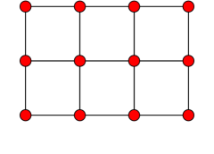
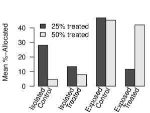
Figure 1: Example illustrating how simple random treatment assignment on a network can lead to very different allocations of nodes to network exposure conditions. Panel (a) gives an example grid network of twelve nodes. Panel (b) gives the average allocation across exposure conditions given simple random assignment to treatment of both three (i.e., 25%) and six (i.e., 25%) nodes.

2.1 Design is Dependent on a Model of Propagation

Let $Z_{i}=1$ if subject $i$ is assigned to the treatment condition and $Z_{i}=0$ if $i$ is assigned to control. In the classical experimental framework, a counterfactual causal effect for a person $i$ is defined through the comparison of that person’s outcome, $Y_{i}(Z_{i}=1)$ under one treatment to that same person’s outcome under a different treatment $Y_{i}(Z_{i}=0)$, given at the same moment in time (Neyman 1990; Rubin 1980; Holland 1986). If potential outcomes under different treatments differ, $Y_{i}(Z_{i})\neq Y_{i}(Z^{\prime}_{i})$ for $Z_{i}\neq Z^{\prime}_{i}$, we say the treatment had an effect. Implicit in this comparison for a single person is the presumption that subject $i$’s outcome only depends on $i$’s treatment status $Z_{i}$ and not on any other $Z_{j}$ — that there is no interference between the treatment or outcomes of person $i$ and those of any other person. Such implicit assumptions are incompatible with the goals of researchers seeking to understand the important causal role played by networks in real world processes. Analysis of experiments on social networks cannot assume away interference, especially if a scholar desires to learn about propagation processes. However, once the assumption of no interference is relaxed, a theoretical model of interference represents a valuable tool to guide the search for propagation’s footprint and to calibrate the experimental design. One method to deal with interference would be to specify the potential outcomes for each unit as a function of the entire treatment assignment to all nodes (Bowers et al. 2013). Such a method is powerful, but it can be theoretically demanding to specify a model for each unit’s outcome. As Aronow and Samii (2017b) show, it is not strictly necessary to assume a theoretical model of interference in order to identify interference effects by instead looking at broad classes of interference. Nevertheless, in both scenarios, a theoretical model of interference is needed to identify the interference effects for which the researcher intends to test, which, in turn, can inform the design of the experiment.

While having differing statistical motivations, the methods of Aronow and Samii (2017a) and Bowers et al. (2013) both require that the researcher draw upon a theoretical model of interference to properly analyze the outcome $Y$. In Aronow and Samii (2017a), a model of interference must be used to identify the exposure conditions (e.g., adjacent to a treated unit, 2 degrees of separation from a treated unit, etc.) to be compared in the study. The model used with the methods of Aronow and Samii (2017a) need not provide precise predictions about to which nodes the treatment will propagate and how, but the model must be complete enough to identify the groups of nodes for which different potential outcomes will be observed under a given direct treatment assignment regime. For the methods proposed by Bowers et al. (2013), a precise analytic model of interference must be specified. The approach adjusts the observed data by removing effect of the treatment as specified by a parametric model of effects, including both direct and indirect effects. If the model captures the true treatment effects, outcome and treatment assignment should be statistically independent for any test statistic. This statistical independence can be tested by permuting the treatment assignment labels, computing a test statistic for each assignment, and comparing the test statistic of the adjusted data to the distribution of test statistics. As the adjusted data must be constructed from a model, it is not possible to use the methods of Bowers et al. (2013) without specifying the precise role of interference in the study.

The need to specify a model of propagation in order to identify an efficient experimental design leads us to question where researchers might start in developing such models. There is a vibrant literature, primarily in the fields of physics and applied mathematics, on graph dynamics, that provides several excellent starting points for analytical models of propagation. These models include the susceptible-infected-recovered disease epidemic models (Kermack 1927; Anderson 1982; Hethcote 2000; Daley 2005), the Bass Diffusion Model (Bass and Jain 1994; Lenk and Rao 1990) and the Hopfield network (Hopfield 1982) and the voter model (Clifford 1973; Liggett 1997; Durrett 1991). In the simulation study that follows, we present and use a variant of the Ising model, a model that contains several of those mentioned above as special cases (Gallavotti 1999). The Ising model is a general formulation for stochastic binary-state dynamics. The classic Ising model has been used quite widely to characterize opinion dynamics (e.g., Vazquez et al. 2003; Fortunato 2005; Sousa et al. 2008; Biswas and Sen 2009).

3 Simulation Study

In what follows we conduct a simulation study in which we evaluate the statistical power of the methods proposed by Aronow and Samii (2017a) and Bowers et al. (2013). The objective of this simulation study is to demonstrate that the statistical power of these procedures depends upon design parameters that are intuitively meaningful in the context of propagation, and that power is maximized at design parameters that differ considerably from those commonly used in experiments without interference — random uniform division of the sample into half control and half treatment. It is outside the scope of the current study to compare the merits of the methods proposed by Aronow and Samii (2017a) with those proposed by Bowers et al. (2013): further, we see the two approaches as complementary in the same way that hypothesis testing and estimation complement one another. We hope that our simulation will illustrate the importance and feasibility of simulation analysis for parameterizing designs for studies of propagation in networks. Throughout this simulation we use the Ghana voter registration station network from Ichino and Schündeln (2012) as our example network. We create a network from the map of roads connecting the registration stations. Two registration stations are considered to be tied if they are within 20km of each other on the road network. This results in a network with 868 vertices, and a density of 2.2%. The network is depicted in Figure 5.

3.1 Simulation Parameters and Definitions

We denote the treatment assigned to vertex $i$ as $Z_{i}\in\{0,1\}$ and the vector of treatment assignments to all vertices as $\mathbf{Z}=(Z_{1},\ldots,Z_{n})^{T}$. The fixed potential outcome of vertex $i$ that would be shown under treatment vector $\mathbf{Z}$ is denoted $Y_{i}(\mathbf{Z})$. Under the sharp null of no treatment effect, all potential outcomes are equal; $Y_{i}(\mathbf{Z})=Y_{i}(\mathbf{Z}^{\prime})=Y_{i}(\{Z_{i}=1,\mathbf{Z}_{-i}\})=Y_{i}(\{Z_{i}=0,\mathbf{Z}^{\prime}_{-i}\})~{}~{}\forall\mathbf{Z}\neq\mathbf{Z}^{\prime}$ and where $-i$ means "all vertices not $i$". $Y_{it}(D_{it})$ is the potential outcome of vertex $i$ at time $t$ under exposure condition $D_{it}$. The exposure condition indicates a mapping of the graph topology and $\mathbf{Z}$ into the categories of exposure defined by the researcher (e.g., directly treated and not tied to any directly treated vertices, not directly treated and adjacent to at least one directly treated node).

	A	B	C	D	E	F
A	0	1	1	0	0	0
B	1	0	0	0	0	0
C	1	0	0	0	0	1
D	0	0	0	0	1	0
E	0	0	0	1	0	0
F	0	0	1	0	0	0

Table 1: Adjacency matrix of a simple 6 node network with 4 edges.

To motivate this discussion, and introduce the primary statistical method, we introduce a toy example using a simpler model and test statistic than will be later employed. The primary goal of this toy example is demonstrate how the power, the probability of rejecting a false null hypothesis, of the statistical approach can depend heavily on the treatment assignment mechanism, the network, and the interaction of these two features in generating the observed outcome. Table 1 shows the adjacency matrix of this simple network. We label this network $S$. Additionally, for each node we have a background covariate $\mathbf{x}=(2.4,0.6,2.2,0.9,0.4,0)^{\prime}$. The covariate and the network combine with the treatment assignment $\mathbf{Z}$ in two outcome models:

$$\mathbf{Y}(\mathbf{Z}) =\mathbf{x}+\theta\mathbf{Z}$$ (1)

$$\mathbf{Y}(\mathbf{Z}) =\mathbf{x}+\theta\mathbf{Z}+(1-\mathbf{Z})\theta I(S\mathbf{Z}>0)$$ (2)

In the first model, as each node’s outcome depends only on its own treatment status, this model involves no spillover. The second model, on the other hand, treated units share their benefit with any untreated neighbors. For simplicity, we fix the true $\theta$ at 1 in both models. To constrast different assignment mechanisms, we consider two treatment assignment mechanisms: assign two units to treatment, four to control (“unbalanced”); three units to treatment, three to control (“balanced”). For each possible treatment strategy, we can enumerate all possible treatment allocation (15 for the unbalanced case and 20 for the balanced case). For each allocation, we can generate the $\mathbf{Y}$ that would be observed if $\theta=1$. For each of these observed $\mathbf{Y}$, we then apply the randomization inference procedure, using a squared t-statistic, to compute $p$-values for the (false) hypothesis that treatment had no effect (i.e., $\theta=0$). This results in a $p$-value that would be observed for each possible randomization. For a given $\alpha$-level, the randomization method that has more $p$-values less than $\alpha$ has higher power.

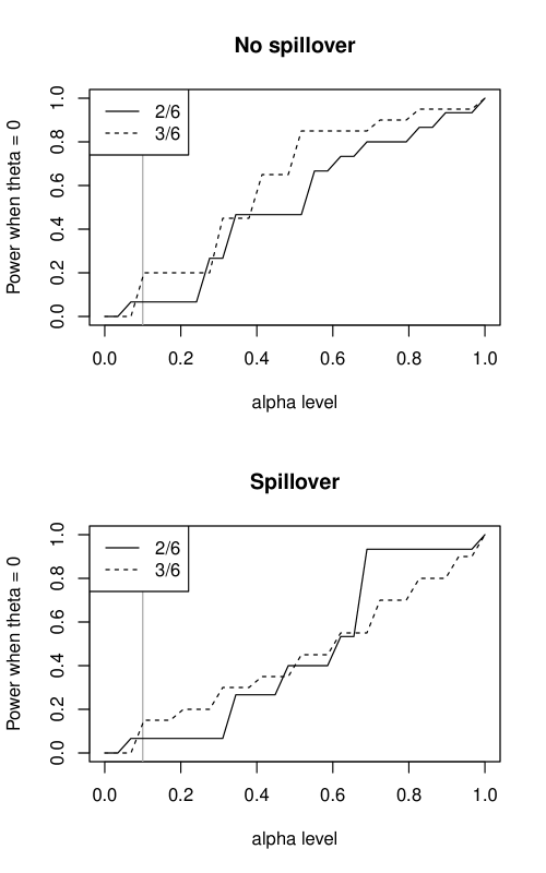
Figure 2: Proportion of randomizations that would reject the null hypothesis that $\theta=0$ when $\theta=1$ (“power”) of the two assignment methods (assigning 2 out of 6 or 3 out of 6 subjects to treatment) as a function of the $\alpha$-level employed. The top panel represent the case of the model of direct effects only, while the lower panel adds an indirect effect for any node that has at least one treated neighbor. The vertical gray line is at $\alpha=0.10$

.

Figure 2 compares the two assignment methods when spillover is and is not present with respect to power, as a function of the selected $\alpha$-level. As the figure shows, in the absence of spillover, the balanced design almost always possess better power characteristics than the unbalanced design. As power is a function of $p$-values generated for each randomization, it can be useful to consider the mean $p$-value of the sharp null hypotheses for these different methods, where lower mean $p$-values correspond to more power. Overall, for the balanced design the average $p$-value without spillover was $0.4$ while for the unbalanced design had mean $p$-values of $0.493$. Conversely, when spillover is present the unbalanced design generally has superior power to the balanced design, with an overall mean of $0.547$ compared to $0.56$ for the balanced design. While the difference between the $p$-values for the spillover model is small, it is important to note that conventional wisdom holds that balanced designs always possess superior power advantages. When spillover is present, however, this is not universally true. In some situations, when spillover is present, unbalanced assignment can increase statistical efficiency.

To investigate this phenomenon in a more realistic setting, in the subsequent simulations we employ a much richer model of treatment effects as well as test statistics that have proven themselves useful in network settings. The model we use for treatment propagation in our simulations is a variant of the Ising Model. The initial treatment assignment of each vertex is drawn independently from $Z_{i}\sim\text{Bernoulli}(\alpha)$. The infection probability—the probability that treatment “infects,” or propagates to, a control vertex—at each iteration of propagation is

$$\frac{1}{1+\exp(\frac{2}{F}(k_{i}-2m_{i}))},$$

where $k$ is number of (directly adjacent) neighbors, $m$ is the number of previously exposed neighbors ($0\leq m_{i}\geq M$), $F$ is a “temperature” parameter that governs the extent to which the propensity to be infected depends on the infection rate among $i$’s neighbors. We initialize the model by assigning treatment ($t=0$), and then we run the propagation model for just one time period ($t=1$). The Ising model controls actual infection after an experimenter assigns $Z_{i}$ at $t=0$. By only producing one iteration of the model, we thus only allow interference at one step or degree in the network.

We specify the potential outcomes of the vertices in our simulation according to the following scheme depending upon the infection status at a given time point. We denote this by $Y(Z_{i,t=0},Z_{i,t=1})$, in which $Z_{i0}\equiv Z_{i,t=0}$ indicates $i$’s initial treatment status and $Z_{i1}$ indicates whether treatment propagates to $i$ at time 1. In the simulation study we consider both multiplicative and additive effects, and propagation models in which treatment propagates stochastically according to the Ising model, and propagates with certainty from directly treated units to their direct neighbors. We generate a baseline (pre-treatment) response $Y(0,0)\sim U(0,1)$ to represent the state of the graph in the absence of any experiment. Our multiplicative treatment effect model changes the baseline in the same, multiplicative, way regardless of the time or manner of “infection” (directly assigned by researcher or propagated from a neighbor), and $Y(1,0)=Y(0,1)=\lambda Y(0,0)$. In the additive treatment effect model $Y(1,0)=Y(0,1)=\lambda+Y(0,0)$. We consider values of $\lambda\in\{0.26,0.63\}$, which correspond to approximately one and two standard deviation shifts in the mean of a standard uniform random variable, and simulate 1,000 treatment propagation and outcome sets at each combination of $F\in\{0,10,\ldots,100\}$ and $\alpha\in\{0.05,0.10,\ldots,0.50\}$.

3.2 Application of Inference Methods

Aronow and Samii’s (2017a) method requires that we define exposure conditions (which include assignment to treatment and also the probability of exposure to a treatment via the network). We define the exposure conditions with respect to what a researcher would be able to observe from the experimental design, assuming the network were observed, and the response. Importantly, in defining the exposure conditions of interest, we assume that the researcher does not exactly know the set of vertices to which the treatment has propagated. We see this as more realistic than a situation in which the researcher knows exactly where the treatment has propagated.

We define the following three distinct exposure conditions, differentiating between those vertices treated initially ($d_{1}$), those vertices that are untreated initially and are adjacent to at least one treated vertex ($d_{(0,1)}$), and those vertices that are untreated initially and are not adjacent to any treated vertices ($d_{(0,0)}$).

• $d_{1}\equiv D_{i}(Z_{i}=1,0\leq m_{it}\geq M)$

• $d_{(0,0)}\equiv D_{i}(Z_{i}=0,m_{it}=0)$

• $d_{(0,1)}\equiv D_{i}(Z_{i}=0,m_{it}\geq 1)$

Figure 3 gives a visual example of a subgraph drawn from the Ghana road network. In the study of the Aronow and Samii (2017a) methods, we focus on identifying the difference between the $d_{(0,1)}$ and $d_{(0,0)}$ conditions.

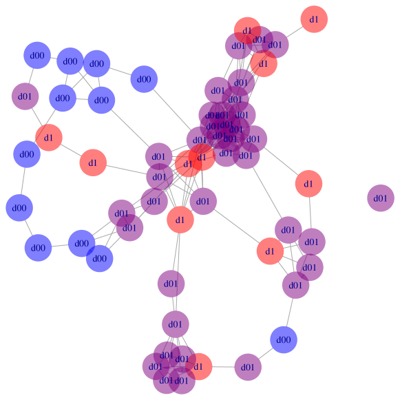
Figure 3: Illustration of exposure conditions for a subgraph of the Ghana road network. One draw from the Ising propagations with $\text{pr}(Z_{i}=1)\sim\text{Bernoulli}(.15)$ for $t\in\{0,1\}$ and Temperature$=10$.

The Aronow and Samii (2017a) estimand is the difference between vertices in two exposure conditions. First, let

$$\hat{\mu}(d_{k})=\frac{1}{n}\sum_{i=1}^{n}\text{\bf I}(D_{i}=d_{k})\frac{Y_{i}(d_{k})}{\pi_{i}(d_{k})},$$

be the estimator of the mean potential outcome among vertices in exposure condition $d_{k}$, where $\pi_{i}(d_{k})$ is the probability that vertex $i$ ends up in condition $d_{k}$. Then the estimator of the difference between potential outcomes in the two exposure conditions is

$$\hat{\tau}(d_{(0,1)},d_{(0,0)})=\hat{\mu}(d_{(0,1)})-\hat{\mu}(d_{(0,0)}).$$

Following Horvitz and Thompson (1952), Aronow and Samii (2017a) show that
$\text{Var}(\hat{\tau}(d_{(0,1)},d_{(0,0)}))\leq 1/N^{2}\left(\text{Var}(\hat{\mu}(d_{(0,1)}))+\text{Var}(\hat{\mu}(d_{(0,0)}))\right)$. In the interest of brevity, we do not re-produce the full variance estimators, but refer readers to Aronow and Samii (2017a). A power analysis gauges the probability that a hypothesis (usually the null hypothesis) is rejected when it is false. In the results that follow, we assess the power to reject $H_{0}:\tau=0$ at the 0.05 significance level.

We test hypotheses about effects following Bowers et al. (2013) using the Anderson-Darling $k$-sample test statistic (Scholz and Stephens 1987) to compare the outcome distributions of vertices in the three different exposure conditions. Following the norms of assessing power against truth, we test hypotheses generated by the correct Ising model and record the amount of false rejections as the parameter values of $\lambda$ and $F$ move away from their true values. The values of the parameters $\lambda$ and $F$ are manipulated to test the null of no effects (i.e., $\lambda=1,F=\infty$) in order to assess power. In the case of the methods proposed by Bowers et al. (2013), we assess power with respect to two different null hypotheses. The first is the null of no effects across all three exposure conditions (i.e., the null that the experiment did not effect any vertices). The second null hypothesis is the null of no difference between $d_{(0,1)}$ and $d_{(0,0)}$ (i.e., the null that there is no interference in that there is no difference between isolated controls and controls that are adjacent to treated vertices).

3.3 Results

The results from the Aronow and Samii (2017a) tests are reported in Figure 4. Three distinct sets of results are presented: (a) those with a multiplicative effect and stochastic propagation (i.e., $Y(1,0)=Y(0,1)=\lambda Y(0,0)$), (b) those with an additive effect (i.e., $Y(1,0)=Y(0,1)=\lambda+Y(0,0)$), and (c) those with an additive effect and certain propagation (i.e., $Y(0,1)=Y(d_{(0,1)})$). We note three characteristics of our results. First, the tests exhibit fairly low power overall, hitting a maximum of approximately 0.8, but sitting below and often far below 0.5. Second, the most powerful design is that in which $\alpha=0.05$, the smallest proportion assigned to initial treatment. Third, as indicated by the relationship of power with the $x$-axis of the plots in panels (a) and (b), the larger the sample of vertices in the $d_{(0,1)}$ condition that are actually exposed to treatment in period one, as governed by the temperature parameter, the more powerful the tests.

$\lambda$ = 0.26	$\lambda$ = 0.63
(a) Multiplicative Effects ($Y(1,0)=Y(0,1)=\lambda Y(0,0)$)
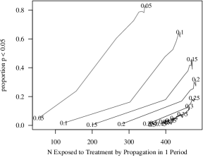
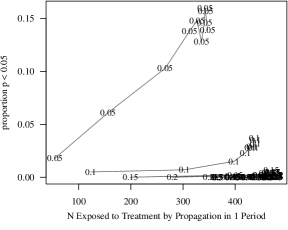
(b) Additive Effects ($Y(1,0)=Y(0,1)=\lambda+Y(0,0)$)
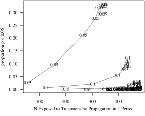
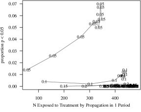
(c) Perfect Propagation ( $Y(0,1)=Y(d_{0,0})$)

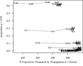
Figure 4: Power Results: Aronow and Samii (2017a) test. Lines are labeled by the proportion assigned to treatment. High power depends on low proportions assigned to treatment. The network contains a total of 868 nodes. The $y$-axes show that nominal power of .8 is not always attained in all designs.

If a researcher wants to estimate the network exposure weighted average causal effect developed by Aronow and Samii (2017a) these kinds of results raise the question about whether the best approach to randomization of treatment assignment is simple uniform assignment without any blocking or use of information about the fixed network. To investigate this we study how power depends on the correlation between $m$ and $Z_{i0}$ (i.e., the correlation between vertex degree and the initial treatment assignment) in the simulation condition with the multiplicative effects and stochastic propagation. The networks depicted in Figure 5 represent examples of treatment assignments biased in favor of high degree vertices (a) and low degree vertices (b). The degree-treatment correlation results are given in Figure 6. We can see in Figure 6 that at each $\alpha$ value there is a strong positive relationship between the degree-treatment correlation and statistical power. This indicates that for the Ghana network structure and the propagation/effects models we have specified, designs that bias treatment assignment towards higher degree nodes would exhibit greater statistical power. This finding generalizes what we know about the use of prognostic background covariates to increase power in randomized experiments to the situation where network degree can be thought of as a moderator of treatment effects.

(a) Treating High Centrality Nodes

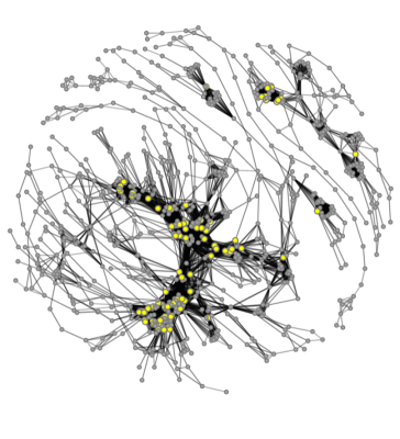
(b) Treating Low Centrality Nodes

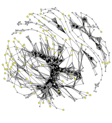
Figure 5: Examples of treatment assignment to either high or low degree nodes in the Ghana 2008 Voter Registration Fraud Experiment network. Vertices are registration stations and yellow nodes are assigned to initial treatment.

Figure 6: When node degree is correlated with probability of treatment assignment, the power to detect indirect effects increases. Results are drawn from the simulation condition with the multiplicative model of effects, and stochastic propagation of treatment.

The results from the model-testing methods of Bowers et al. (2013) in Figures 7–9 differ in their implications from the results based on estimation. First, the power in these tests is much higher overall. This makes some sense: we are assessing the ability of the test to reject false parameters given a correct propagation model, a good test should eventually reject values of parameters that are distant from the truth. The methods focused on differences of averages do not include much information about the propagation model except as a weight arising indirectly from what we can observe, so those procedures have less information to use in statistical inference in this simulation study. Second, when we focus on the test of the sharp null of no effects when all three exposure conditions are included, we see that the low values of $\alpha$ exhibit low power. However, when the test compares only $d_{(0,1)}$ against $d_{(0,0)}$, which can be considered a test for propagation effects (i.e., excluding directly treated vertices), the lower $\alpha$ designs perform better. This tradeoff between the power to detect any effect versus the power to detect propagated effects replicate the findings from Bowers et al. (2013): in order to learn about propagation, one should assign relatively few nodes to treatment, in order to test an overall null of no effects, then more power arises from more directly assigned-to-treatment nodes. There is also a positive association between the number of vertices in the $d_{(0,1)}$ condition that are exposed to treatment by period one and the power of the tests. This last result arises from the fact that, when few in the $d_{(0,1)}$ condition are exposed to treatment, the $d_{(0,1)}$ outcomes are, in large part, equivalent to the $d_{(0,0)}$ outcomes.

Figure 7: Power with multiplicative effects model and true Ising propagation model following Bowers et al. (2013).

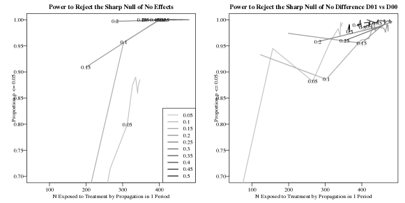
Figure 8: Power with additive effects model and true Ising propagation model following Bowers et al. (2013).

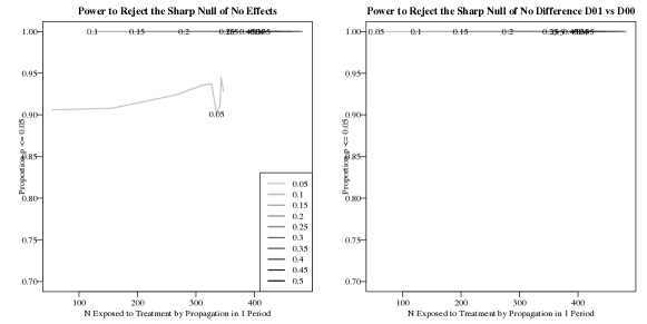
Figure 9: Power with additive effects and perfect propagation and true Ising propagation model following Bowers et al. (2013).

3.4 Summary

We have shown that learning about a simple model of propagation of treatment through a network (via comparisons of nodes possibly indirectly exposed to the treatment with nodes not exposed to treatment) can be enhanced when relatively few of the nodes in a network are assigned treatment. We also find, at least with the Aronow and Samii method, that power may be improved by using network structure in formulating the randomization distribution (e.g., assigning treatment to vertices with probability proportional to their degrees in the network). Both the Bowers et al. method and the Aronow and Samii method explicitly account for the randomization distribution, and we are, as such, not concerned about introducing bias into the methodology by biasing the randomization distribution. This would be a particularly important method if the researcher hypothesized that the model of effects varied with respect to network structure (e.g., a hypothesis that higher degree vertices are more susceptible to the treatment). Since the randomization distribution is incorporated into the methods we present, both approaches could be used to test hypotheses regarding effects that vary with respect to network structure. More abstractly, our analysis acts an example for those desiring to evaluate their own models of propagation on networks and experimental designs before going into the field. Indeed, our findings that the power-maximizing proportion assigned to treatment falls well below 0.50, and power can be increased by disproportionately assigning treatment to higher degree nodes is specific to the network dynamics that we artificially designed for this simulation study (i.e., the Ghana road network structure, the Ising model for treatment propagation, and our model(s) of effects). However, simulation studies such as the ones we have run would assist the researcher in optimally designing the experiment given a network structure, and model(s) that characterized propagation and treatment effects. We do not consider our findings regarding the proportion assigned to treatment and disproportionate assignment to highly connected nodes to apply universally to experiments on networks.

We have not shown how the Bowers et al. (2013) approach performs when an incorrect model is assessed. We did not do this because we are focusing on design—and power analysis requires that we create a truth against which to compare alternatives. Bowers et al. (2013, 2016) show that, in the analysis stage, hypothesis tests may have very low or no power if the model being assessed has no bearing on the underlying mechanism, but we are not certain what kind of design advice would follow from such findings—merely increasing the size of a fixed network may be impossible.

We have also not considered, for either the Aronow and Samii or Bowers et al. methods, how design affects statistical power when there is uncertainty regarding the network structure. To incorporate uncertainty regarding the network, a stochastic model for the network would need to be integrated into the analytical procedure(s) (e.g., Desmarais and Cranmer 2012). Relatedly, network-based sampling methods (e.g., snowball sampling) are commonly used to study hard-to-reach populations (e.g., illicit drug users (Wang et al. 2007)). If researchers are introducing interventions in network-based samples, the effects of the interventions may include interference. There is an active literature in statistics and computer science that considers the ways in which network quantities (e.g., prevalence of a behavior, degree distribution) can be accurately and efficiently estimated via network sampling designs (Handcock and Gile 2010; Kurant et al. 2012; Gile and Handcock 2010). We have not thoroughly considered how the tests studied in the current paper, and associated approaches to treatment assignment, would perform in the context of network sampling, but future work should consider the integration of tests for and estimates of interference effects with network sampling designs. Such consideration would involve the assessment of optimal treatment assignment distributions (e.g., disproportionately treating higher degree nodes) based on noisy information regarding network structure, gathered through a network sampling design.

4 Conclusion

We describe the challenges in experimental design that arise when the researcher is interested in studying the process of propagation on a network with the objective of drawing causal inference. The experimental designs that work most effectively in experiments in which there is no interference are unlikely to be directly transferable to experimental research on propagation. We review two recently developed frameworks for statistical inference regarding interference in networks. One commonality we draw from these two frameworks is that theoretical analytic models of propagation play a key role in their application, which means that substantive theory about the nature of treatment effects and network relations features more prominently in the statistical analysis of experimental data generated for the study of propagation than in the classical, non-interference, experimental framework.

We present a simulation study to (1) illustrate how simulation can be a useful guide in identifying design parameters for experimental studies of interference, and (2) study the properties of the two frameworks for statistical inference presented in the front end of the paper. Three findings from the simulation study are notable. First, statistical power depends upon design parameters and, for example, the optimal proportion assigned to initial treatment may be much lower than the conventionally applied 0.5. Second, the relationship between design parameters and power depends upon the framework for statistical inference. Third, our results regarding the positive relationship between the degree-treatment correlation and power indicates that randomization designs that take into account graph topology are likely to exhibit substantial power gains over uniform randomization designs. It is important to note, however, that these findings are specific to our simulation setup, and may not apply directly to other network experiments defined by different networks, models of propagation, and/or models of treatment effects. Nevertheless, the results from the simulation study underscore the importance of considering design parameters for experimental studies of propagation, as the standards of the classical experimental framework are unlikely to apply. We encourage the use of such simulation studies to guide the design of experiments on networks.

Our results suggest three fruitful directions for future research. First, as noted above, the literature on network dynamics offers several possibilities for specifying models of propagation on networks. Researchers may not have strong a priori theory regarding the functional form of the propagation model. This leads to the first future direction—considering whether the propagation model can be learned algorithmically, or analyzed though a nonparametric framework. Second, although we focused on power to detect indirect and direct effects, we were studying multiple hypotheses (two in this case). Our work here has made us wonder whether designs to maximize power against combined tests of those (and other) hypotheses might look different from designs which aim only at maximizing power to detect propagation or overall effects. The third question regards the network through which interference occurs. Future work should consider precisely how uncertainty regarding the network structure can be incorporated into the methods we present.

Appendix

$\lambda$ = 0.26	$\lambda$ = 0.63
(a) Multiplicative Effects ($Y(1,0)=Y(0,1)=\lambda Y(0,0)$)
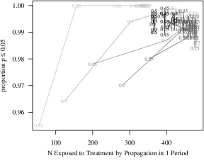
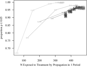
(b) Additive Effects ($Y(1,0)=Y(0,1)=\lambda+Y(0,0)$)
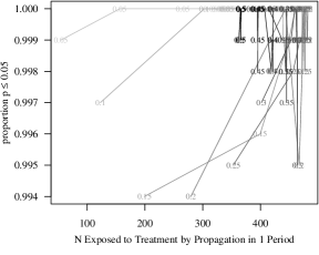
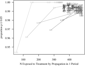
(c) Perfect Propagation ( $Y(0,1)=Y(d_{0,0})$)

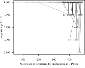
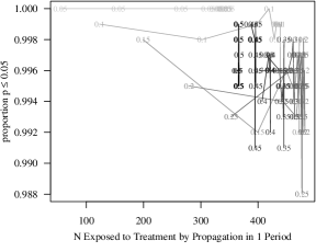
Figure 10: Power Results: Aronow and Samii (2017a) (Hajek) test. Lines are labeled by the proportion assigned to treatment. High power depends on low proportions assigned to treatment. The network contains a total of 868 nodes. The $y$-axes show that the test based on the Hajek estimator exhibits much higher power than the test based on the HT estimator.

References

- Anderson (1982) Anderson, R. M. e. (1982). Population Dynamics of Infectious Diseases: Theory and Applications. Chapman and Hall.
- Aral and Walker (2011) Aral, S. and Walker, D. (2011). Creating social contagion through viral product design: A randomized trial of peer influence in networks. Management Science, 57(9):1623–1639.
- Aronow and Samii (2017a) Aronow, P. M. and Samii, C. (2017a). Estimating average causal effects under general interference, with application to a social network experiment. Annals of Applied Statistics.
- Aronow and Samii (2017b) Aronow, P. M. and Samii, C. (2017b). Estimating spatial effects. Unpublished manuscript.
- Baird et al. (2017) Baird, S., Bohren, J. A., McIntosh, C., and Ozler, B. (2017). Optimal design of experiments in the presence of interference. Review of Economics & Statistics.
- Bapna and Umyarov (2015) Bapna, R. and Umyarov, A. (2015). Do your online friends make you pay? a randomized field experiment on peer influence in online social networks. Management Science, 61(8):1902–1920.
- Bass and Jain (1994) Bass, Frank M.; Krishnan, T. V. and Jain, D. C. (1994). Why the bass model fits without decision variables. Marketing Science, 13(3):204–223.
- Basse and Airoldi (2015) Basse, G. W. and Airoldi, E. M. (2015). Optimal design of experiments in the presence of network-correlated outcomes. arXiv preprint arXiv:1507.00803.
- Biswas and Sen (2009) Biswas, S. and Sen, P. (2009). Model of binary opinion dynamics: Coarsening and effect of disorder. Physical Review E, 80(2):027101.
- Bond et al. (2012) Bond, R. M., Fariss, C. J., Jones, J. J., Kramer, A. D., Marlow, C., Settle, J. E., and Fowler, J. H. (2012). A 61-million-person experiment in social influence and political mobilization. Nature, 489(7415):295–298.
- Bowers et al. (2014) Bowers, J., Fredrickson, M., and Hansen, B. (2014). RItools: Randomization Inference Tools. R package version 0.1-12.
- Bowers et al. (2013) Bowers, J., Fredrickson, M., and Panagopoulos, C. (2013). Reasoning about interference between units: A general framework. Political Analysis, 21(1):97–124.
- Bowers et al. (2016) Bowers, J., Fredrickson, M. M., and Aronow, P. M. (2016). Research note: A more powerful test statistic for reasoning about interference between units. Political Analysis, page mpw018.
- Butler et al. (2011) Butler, D. M., Nickerson, D. W., et al. (2011). Can learning constituency opinion affect how legislators vote? results from a field experiment. Quarterly Journal of Political Science, 6(1):55–83.
- Chen et al. (2010) Chen, J., Humphreys, M., and Modi, V. (2010). Technology diffusion and social networks: Evidence from a field experiment in uganda. Unpublished manuscript.
- Clifford (1973) Clifford, P. A. W. S. (1973). A model for spatial conflict. Biometrika, 60:581–588.
- Coppock (2014) Coppock, A. (2014). Information spillovers: Another look at experimental estimates of legislator responsiveness. Journal of Experimental Political Science, 1(02):159–169.
- Coppock (2016) Coppock, A. (2016). Information spillovers: Another look at experimental estimates of legislator responsiveness corrigendum. Journal of Experimental Political Science, 3(2):206–208.
- Daley (2005) Daley, D. J. s Gani, J. (2005). Epidemic Modeling: An Introduction. NY: Cambridge University Press.
- Desmarais and Cranmer (2012) Desmarais, B. A. and Cranmer, S. J. (2012). Statistical inference for valued-edge networks: the generalized exponential random graph model. PloS one, 7(1):e30136.
- Durrett (1991) Durrett, Richard; Kesten, H. (1991). Random walks, Brownian motion, and interacting particle systems. Springer.
- Eckles et al. (2017) Eckles, D., Karrer, B., and Ugander, J. (2017). Design and analysis of experiments in networks: Reducing bias from interference. Journal of Causal Inference, 5(1).
- Fortunato (2005) Fortunato, S. (2005). The sznajd consensus model with continuous opinions. International Journal of Modern Physics C, 16(01):17–24.
- Gallavotti (1999) Gallavotti, G. (1999). Statistical mechanics: A short treatise. Springer, New York.
- Gerber and Green (2012) Gerber, A. S. and Green, D. P. (2012). Field experiments: Design, analysis, and interpretation. WW Norton.
- Gile and Handcock (2010) Gile, K. J. and Handcock, M. S. (2010). Respondent-driven sampling: an assessment of current methodology. Sociological methodology, 40(1):285–327.
- Handcock and Gile (2010) Handcock, M. S. and Gile, K. J. (2010). Modeling social networks from sampled data. The Annals of Applied Statistics, 4(1):5.
- Hethcote (2000) Hethcote, H. W. (2000). The mathematics of infectious diseases. Society for Industrial and Applied Mathematics, 42:599–653.
- Hirano and Hahn (2010) Hirano, K. and Hahn, J. (2010). Design of randomized experiments to measure social interaction effects. Economics Letters, 106(1):51–53.
- Holland (1986) Holland, P. W. (1986). Statistics and causal inference. Journal of the American Statistical Association, 81(396):945–960.
- Hopfield (1982) Hopfield, J. (1982). Neural networks and physical systems with emergent collective computational abilities. Proceedings of the National Academy of Sciences, 79(8):2554–2558.
- Horvitz and Thompson (1952) Horvitz, D. G. and Thompson, D. J. (1952). A generalization of sampling without replacement from a finite universe. Journal of the American Statistical Association, 47(260):663–685.
- Hudgens and Halloran (2008) Hudgens, M. and Halloran, M. (2008). Toward causal inference with interference. Journal of the American Statistical Association, 103(482):832–842.
- Ichino and Schündeln (2012) Ichino, N. and Schündeln, M. (2012). Deterring or displacing electoral irregularities? spillover effects of observers in a randomized field experiment in ghana. The Journal of Politics, 74:292–307.
- Kermack (1927) Kermack, W. O.; McKendrick, A. G. (1927). A contribution to the mathematical theory of epidemics. Mathematical, Physical and Engineering Sciences, 115(772):700.
- Kurant et al. (2012) Kurant, M., Gjoka, M., Wang, Y., Almquist, Z. W., Butts, C. T., and Markopoulou, A. (2012). Coarse-grained topology estimation via graph sampling. In Proceedings of the 2012 ACM workshop on Workshop on online social networks, pages 25–30. ACM.
- Lenk and Rao (1990) Lenk, P. J. and Rao, A. (1990). New models from old: Forecasting product adoption by hierarchical bayes procedure. Marketing Science, 9(1):42–53.
- Liggett (1997) Liggett, T. M. (1997). Stochastic models of interacting systems. The Annals of Probability, 25(1):1–2.
- Lyons (2011) Lyons, R. (2011). The spread of evidence-poor medicine via flawed social-network analysis. Statistics, Politics, and Policy, 2(1).
- Miguel and Kremer (2004) Miguel, E. and Kremer, M. (2004). Worms: identifying impacts on education and health in the presence of treatment externalities. Econometrica, 72(1):159–217.
- Neyman (1990) Neyman, J. (1923 [1990]). On the application of probability theory to agricultural experiments. essay on principles. section 9 (1923). Statistical Science, 5:463–480. reprint. Transl. by Dabrowska and Speed.
- Nickerson (2008) Nickerson, D. (2008). Is voting contagious? evidence from two field experiments. American Political Science Review, 102(01):49–57.
- Nickerson (2011) Nickerson, D. (2011). Social networks and political context. Cambridge Handbook of Experimental Political Science, page 273.
- Ostrovsky and Schwarz (2011) Ostrovsky, M. and Schwarz, M. (2011). Reserve prices in internet advertising auctions: a field experiment. In Proceedings of the 12th ACM conference on Electronic commerce, EC ’11, pages 59–60, New York, NY, USA. ACM.
- Rubin (1980) Rubin, D. B. (1980). Randomization analysis of experimental data: The fisher randomization test comment. Journal of the American Statistical Association, 75(371):591–593.
- Scholz and Stephens (1987) Scholz, F. W. and Stephens, M. A. (1987). K-sample anderson-darling tests. Journal of the American Statistical Association, 82(399):918–924.
- Shalizi and Thomas (2011) Shalizi, C. R. and Thomas, A. C. (2011). Homophily and Contagion Are Generically Confounded in Observational Social Network Studies. Sociol Methods Res, 40(2):211–239.
- Sinclair (2011) Sinclair, B. (2011). Design and analysis of experiments in multilevel populations. In Cambridge Handbook of Experimental Political Science, page 906. Cambridge University Press.
- Sinclair et al. (2012) Sinclair, B., McConnell, M., and Green, D. P. (2012). Detecting spillover effects: Design and analysis of multilevel experiments. American Journal of Political Science, 56(4):1055–1069.
- Sobel (2006) Sobel, M. (2006). What do randomized studies of housing mobility demonstrate? Journal of the American Statistical Association, 101(476):1398–1407.
- Sousa et al. (2008) Sousa, A., Yu-Song, T., and Ausloos, M. (2008). Effects of agents’ mobility on opinion spreading in sznajd model. The European Physical Journal B-Condensed Matter and Complex Systems, 66(1):115–124.
- Tchetgen and VanderWeele (2010) Tchetgen, E. and VanderWeele, T. (2010). On causal inference in the presence of interference. Statistical Methods in Medical Research.
- Toulis and Kao (2013) Toulis, P. and Kao, E. (2013). Estimation of causal peer influence effects. In Proceedings of the 30th International Conference on Machine Learning, ICML ’13.
- VanderWeele (2008) VanderWeele, T. (2008). Ignorability and stability assumptions in neighborhood effects research. Statistics in medicine, 27(11):1934–1943.
- VanderWeele (2010) VanderWeele, T. (2010). Direct and indirect effects for neighborhood-based clustered and longitudinal data. Sociological Methods & Research, 38(4):515.
- VanderWeele and Tchetgen (2011) VanderWeele, T. and Tchetgen, E. (2011). Bounding the infectiousness effect in vaccine trials. Epidemiology, 22(5):686–693.
- VanderWeele et al. (2011) VanderWeele, T., Tchetgen, E., and Halloran, M. (2011). Components of the indirect effect in vaccine trials: identification of contagion and infectiousness effects. COBRA Preprint Series, page 85.
- VanderWeele and Tchetgen Tchetgen (2011) VanderWeele, T. and Tchetgen Tchetgen, E. (2011). Effect partitioning under interference in two-stage randomized vaccine trials. Statistics & probability letters, 81(7):861–869.
- VanderWeele et al. (2012) VanderWeele, T., Vandenbroucke, J., Tchetgen Tchetgen, E., and Robins, J. (2012). A mapping between interactions and interference: implications for vaccine trials. Epidemiology, 23(2):285.
- Vazquez et al. (2003) Vazquez, F., Krapivsky, P. L., and Redner, S. (2003). Constrained opinion dynamics: Freezing and slow evolution. Journal of Physics A: Mathematical and General, 36(3):L61.