Wire constructions of Abelian topological phases in three or more dimensions

Abstract

Coupled-wire constructions have proven to be useful tools to characterize Abelian and non-Abelian topological states of matter in two spatial dimensions. In many cases, their success has been complemented by the vast arsenal of other theoretical tools available to study such systems. In three dimensions, however, much less is known about topological phases. Since the theoretical arsenal in this case is smaller, it stands to reason that wire constructions, which are based on one-dimensional physics, could play a useful role in developing a greater microscopic understanding of three-dimensional topological phases. In this paper, we provide a comprehensive strategy, based on the geometric arrangement of commuting projectors in the toric code, to generate and characterize coupled-wire realizations of strongly-interacting three-dimensional topological phases. We show how this method can be used to construct pointlike and linelike excitations, and to determine the topological degeneracy. We also point out how, with minor modifications, the machinery already developed in two dimensions can be naturally applied to study the surface states of these systems, a fact that has implications for the study of surface topological order. Finally, we show that the strategy developed for the construction of three-dimensional topological phases generalizes readily to arbitrary dimensions, vastly expanding the existing landscape of coupled-wire theories. Throughout the paper, we discuss $\mathbb{Z}^{\,}_{m}$ topological order in three and four dimensions as a concrete example of this approach, but the approach itself is not limited to this type of topological order.

I Introduction

The experimental discovery of the integer and fractional quantum Hall effects excited enormous interest in the study of topological states of matter in two dimensional space. Strongly interacting states of matter distinguished by the presence of excitations with fractional quantum numbers or nontrivial boundary modes have attracted particular attention from theorists. Over time, a vast arsenal of theoretical tools has been developed to study such systems, from the microscopic (e.g., numerical techniques to study lattice models with topologically ordered ground states) to the macroscopic (e.g., topological quantum field theories).

Wire constructions, which were first undertaken for the integer Poilblanc et al. (1987); Yakovenko (1991); Lee (1994), and later the fractional Kane et al. (2002); Teo and Kane (2014); Mong et al. (2014); Klinovaja and Loss (2014); Meng et al. (2014); Klinovaja and Tserkovnyak (2014); Sagi and Oreg (2014); Neupert et al. (2014); Meng and Sela (2014); Klinovaja et al. (2015); Santos et al. (2015); Sagi et al. (2015), quantum Hall effect, are conveniently poised midway between these two extremes. The approach in this case is to model a topological phase by starting from an anisotropic theory of decoupled gapless quantum wires, and then introducing local couplings between the wires to produce a gapped state of matter with an isotropic low-energy description. This approach has the virtue of yielding the edge theory, itself that of a Luttinger liquid, directly, and of providing means to construct the low-lying quasiparticle excitations of the bulk quantum liquid. Furthermore, because wire constructions make use of well-understood techniques in one-dimensional physics, such as Abelian (or non-Abelian) bosonization, one can construct analytically tractable theories of states of matter that might not otherwise admit a controlled analytical description.

In recent years, wire constructions have also been used to study fractional topological insulators (FTIs) Neupert et al. (2014); Sagi and Oreg (2014); Santos et al. (2015) and spin liquids Meng et al. (2015); Gorohovsky et al. (2015), and also to develop an extension Neupert et al. (2014) of the ten-fold way for noninteracting fermions Altland and Zirnbauer (1997); Schnyder et al. (2009); Kitaev (2009); Ryu et al. (2010) to strongly-correlated systems.

Since the prediction Fu et al. (2007) and discovery Hsi ; Hsieh et al. (2009); Che (a) of three-dimensional $\mathbb{Z}^{\,}_{2}$ topological insulators (TIs), there has been a growing interest in understanding topological states of matter in three spatial dimensions. In addition to generalizing these time-reversal invariant $\mathbb{Z}^{\,}_{2}$ topological insulator to the strongly-interacting regime Maciejko et al. (2010); Swingle et al. (2011); Maciejko et al. (2014), there has been an effort to derive effective field theories describing the bulk of such TIs, and to determine the bulk-boundary correspondence in such theories that yields the hallmark single Dirac cone on the two-dimensional surface Cho and Moore (2011); Chan et al. (2013); Tiwari et al. (2014); Ye and Gu (2015); Che (b). Further work has undertaken efforts to understand broader features of three-dimensional topological states of matter, such as the statistics of pointlike and linelike excitations Wang and Levin (2014); Lin and Levin (2015). For example, it has been shown that certain three-dimensional topological phases can only be distinguished by the mutual statistics among three linelike excitations Lin and Levin (2015).

Another major direction of work concerns three-dimensional systems whose surfaces are themselves two-dimensional topological states of matter. The simplest example of this phenomenon occurs on the surface of a $\mathbb{Z}^{\,}_{2}$ TI when time-reversal symmetry is locally broken by a magnetic field on the surface, in which case a half-integer surface quantum Hall effect develops Fu and Kane (2007); Qi et al. (2008); Xu et al. (2014); Yoshimi et al. (2015). Further theoretical work has shown that generic three-dimensional topological phases, including but not limited to the fermionic $\mathbb{Z}^{\,}_{2}$ TI, can exhibit more exotic surface topological phases that cannot exist with the same realization of symmetries for local Hamiltonians in purely two-dimensional space. This family of surface phenomena is known as surface topological order von Keyserlingk et al. (2013); Vishwanath and Senthil (2013); Wang and Senthil (2013); Wang et al. (2013); Burnell et al. (2014); Chen et al. (2014); Metlitski et al. (2015); Mross et al. (2015). Several recent works Mross et al. (2015); Sahoo et al. (2015) have approached the question of surface topological order by applying the quasi-one-dimensional physics of wire constructions, although it appears that this approach necessitates the use of an unusual “antiferromagnetic” time-reversal symmetry rather than the usual (physical) realization of reversal of time, which acts on-site. It is possible that a fully three-dimensional wire construction could remedy this peculiarity, although such a description is still lacking.

Layer constructions, in which planes of two-dimensional topological liquids are stacked on top of one another and coupled, were used to construct the single surface Dirac cone of the three-dimensional $\mathbb{Z}^{\,}_{2}$ TI Hosur et al. (2010) and to study surface topological order Jian and Qi (2014). Wire constructions of three-dimensional topological states of matter have also recently been undertaken, yielding Weyl semimetals Vazifeh (2013); Meng (2015) and a class of fractional topological insulators Sagi and Oreg (2015). However, in all three cases, different methods are used to develop the wire constructions themselves, and little effort has been made to extend these constructions beyond the specific problem at hand in each example. In order to attack the most distinctive aspects of topological states of matter in three dimensions, such as surface topological order, it is therefore necessary to develop a framework that lends itself readily to a variety of approaches with minimal modifications.

In this paper, we provide a comprehensive strategy to design wire constructions of strongly-interacting Abelian topological states of matter in three dimensions. The strategy that we present is to start with decoupled quantum wires placed on the links of a two-dimensional square lattice, and then to couple the wires with many-body interactions associated with each star and plaquette of the lattice. In this way, each interaction term that couples neighboring wires can be viewed as corresponding to one of the commuting projectors that enters Kitaev’s toric code Hamiltonian Kitaev (2003). This correspondence simplifies the application of a criterion, first proposed by Haldane, to ensure that these interaction terms do not compete, and are sufficient in number to gap out all gapless modes in the array of quantum wires when periodic boundary conditions are imposed along all three spatial directions.

When all interaction terms satisfy this criterion, the Hamiltonian is frustration-free, and taking the strong-coupling limit produces a gapped three-dimensional state of matter. With this done, one can proceed to characterize this state of matter in terms of its pointlike and linelike excitations, as well as their statistics, and calculate the topological degeneracy, if any, of the ground-state manifold. The class of three-dimensional models studied in this work features a topological degeneracy given by $|\text{det }\varkappa|^{3}$, where the integer-valued matrix $\varkappa$ contains information about the mutual statistics of pointlike and linelike excitations in the theory. This is in close analogy with the $K$-matrix formalism developed for two-dimensional topological states of matter Wen and Zee (1992). When periodic boundary conditions are relaxed by the presence of two-dimensional terminating surfaces, we further show that gapless surface states result. One can apply the coupled-wire techniques already developed in two dimensions to study the various gapped surface states that can be produced by introducing interwire hoppings or interactions on the surface, provided that the added terms are compatible with the interactions in the bulk.

In addition, we show that the above strategy for constructing three-dimensional Abelian topological states of matter can be readily extended to arbitrary dimensions, vastly expanding the existing scope of the coupled-wire approach. Indeed, much as it is possible to define higher-dimensional versions of the toric code on hypercubic lattices (see, e.g., Ref. Mazáč and Hamma (2012)), one can arrange a set of decoupled quantum wires on a $d$-dimensional hypercubic lattice and couple them with interactions defined on stars and plaquettes of this lattice. Applying Haldane’s compatibility criterion, one can show that these interactions produce a gapped $(d+1)$-dimensional state of matter, whose excitations and topological properties can be investigated much as in the three-dimensional case.

The structure of this paper is as follows. In Sec. II, we develop in detail the strategy discussed above for constructing three-dimensional topological phases from coupled wires. In Sec. II.1, we establish the basic notation used to describe the array of decoupled quantum wires. In Sec. II.2, we present Haldane’s compatibility criterion and a class of many-body interactions between wires that satisfy it. (This class is mainly chosen for analytical expedience, and is not the only class of interactions that can be constructed according to our strategy.) In Sec. II.3, we show how to use the interacting arrays of quantum wires defined in Secs. II.1 and II.2 to study states of matter with fractionalized excitations. In particular, we show how to construct pointlike and linelike excitations, and determine their statistics, as well as the topological ground state degeneracy. Next, in Sec. II.4 we exemplify our strategy with perhaps the simplest type of topological order in three dimensions, namely $\mathbb{Z}^{\,}_{m}$ topological order. Furthermore, we investigate the surface states of these $\mathbb{Z}^{\,}_{m}$-topologically-ordered states of matter, and find that they are unstable to interwire hoppings. Additionally, a surface fractional quantum Hall effect with Hall conductivity $[(2e)^{2}/h]\times(1/2m)$ can develop at the expense of breaking time-reversal symmetry on the surface. We also discuss how these observations regarding surface states can be extended to the more general class of interwire interactions introduced in Sec. II.2.

Next, in Sec. III, we outline the generalization of our results to arbitrary dimensions. In Sec. III.1, we discuss how to define $d$-dimensional hypercubic arrays of quantum wires that are analogous to the square array of quantum wires used to construct three-dimensional topological states. Then, in Sec. III.2, we generalize the results of Sec. II.2 regarding the definitions of appropriate interwire couplings and their compatibility in the strong-coupling limit. Finally, in Sec. III.3, we provide an example of this generalization by constructing $\mathbb{Z}^{\,}_{m}$-topologically-ordered states of matter in four dimensions, and constructing their pointlike, linelike, and membranelike excitations, before concluding in Sec. IV.

II Three-dimensional wire constructions

In this section, a method to construct arrays of coupled wires realizing topological phases of matter in three-dimensional space is presented. We begin by defining a class of gapless theories describing decoupled wires, before moving on to a discussion of interwire couplings. In particular, we provide a set of algebraic criteria that are sufficient to determine whether the theory is gapped when periodic boundary conditions are imposed.

II.1 Decoupled wires

We consider a two-dimensional array of $2N$ quantum wires, labeled by Latin indices $j=1,\dots,2N$, placed on the links of a two-dimensional square lattice embedded in three-dimensional Euclidean space. Each quantum wire is assumed to be gapless and nonchiral, and therefore to contain $2M$ gapless degrees of freedom, labeled by Greek indices $\alpha=1,\dots,2M$. We take the wires (of length $L$) to lie along the $z$-direction, and the square lattice to lie in the $x$-$y$ plane. We will impose periodic boundary conditions in all directions ($x$, $y$, and $z$) until further notice. The set of decoupled quantum wires is described by the quadratic Lagrangian

$$\hat{L}^{\,}_{0}=\frac{1}{4\pi}\int\limits^{L}_{0}\mathrm{d}z\Bigg{[}\left(\partial^{\,}_{t}\hat{\Phi}\right)^{\mathsf{T}}\!\mathcal{K}\left(\partial^{\,}_{z}\hat{\Phi}\right)-\left(\partial^{\,}_{z}\hat{\Phi}\right)^{\mathsf{T}}\!\mathcal{V}\left(\partial^{\,}_{z}\hat{\Phi}\right)\Bigg{]}$$ (1a)

where

$$\begin{split}\hat{\Phi}(t,z)&\,\raisebox{0.85pt}{.}\raisebox{2.85pt}{.}\!\!=\,\Big{(}\hat{\phi}^{\,}_{1,1}(t,z)\ \dots\ \hat{\phi}^{\,}_{1,2M}(t,z)\mid\\ &\qquad\dots\mid\hat{\phi}^{\,}_{2N,1}(t,z)\ \dots\ \hat{\phi}^{\,}_{2N,2M}(t,z)\Big{)}^{\mathsf{T}}\end{split}$$ (1b)

is a vector that collects the $$2M \hat{\phi}^{\,}_{j,\alpha}(t,z) j=1,\ldots,2N 4MN$$ scalar fields defined in each of the wires. We use vertical bars as a visual aid to separate degrees of freedom defined in different wires. The block-diagonal -dimensional matrix

$$\mathcal{K}\,\raisebox{0.85pt}{.}\raisebox{2.85pt}{.}\!\!=\,\mathbbm{1}^{\,}_{2N}\otimes K,$$ (1c)

where $$\mathbbm{1}^{\,}_{2N} 2N K 2M\times 2M$$ is the unit matrix of dimension and is a symmetric matrix with integer entries, yields the equal-time commutation relations

$$\left[\partial^{\,}_{z}\hat{\phi}^{\,}_{j,\alpha}(z),\hat{\phi}^{\,}_{j^{\prime},\alpha^{\prime}}(z^{\prime})\right] =\mathrm{i}\,2\pi\,\delta^{\,}_{jj^{\prime}}\,K^{-1}_{\alpha\alpha^{\prime}}\,\delta(z-z^{\prime}).$$ (1d)

We will omit the explicit time dependence of the fields from now on. Finally, the block-diagonal $$4MN\times 4MN$$ matrix

$$\mathcal{V}\,\raisebox{0.85pt}{.}\raisebox{2.85pt}{.}\!\!=\,\mathbbm{1}^{\,}_{2N}\otimes V,$$ (1e)

where the $$2M\times 2M V V K 4MN$$ matrix is real, symmetric, and positive-definite. The matrix is set by microscopics within each wire, and will usually be taken to be a diagonal matrix in this work. However, the matrix , which enters the commutation relations (1d), contains crucial data that define the fundamental degrees of freedom in a wire. The final data necessary to complete the definition of the theory describing the two-dimensional array of decoupled quantum wires is the -dimensional “charge-vector”

$$\mathcal{Q}\,\raisebox{0.85pt}{.}\raisebox{2.85pt}{.}\!\!=\,\begin{pmatrix}Q&\mid&Q&\mid&\dots&\mid&Q\end{pmatrix}^{\mathsf{T}}.$$ (1f)

The $2M$-dimensional integer vector $Q$ collects the $U(1)$ electric charges associated with the scalar fields $\hat{\phi}^{\,}_{j,\alpha}$, $\alpha=1,\dots,2M$.

The theory defined by Eqs. (1) can be viewed as an effective low-energy description of a two-dimensional array of decoupled physical quantum wires containing fermionic or bosonic degrees of freedom.

For fermions, each wire $j=1,\ldots,2N$ contains $M$ flavors of chiral scalar fields $\hat{\phi}^{\,}_{j,\alpha^{\,}_{R}}$ and $\hat{\phi}^{\,}_{j,\alpha^{\,}_{L}}$, where $\alpha^{\,}_{R,L}=1,\dots,M$ label right- and left-moving degrees of freedom, respectively. These fields obey the chiral equal-time commutation relations

$$\left[\partial^{\,}_{z}\hat{\phi}^{\,}_{j,\alpha^{\,}_{R}}(z),\hat{\phi}^{\,}_{j^{\prime},\alpha^{\prime}_{R}}(z^{\prime})\right] =+\mathrm{i}\,2\pi\,\delta^{\,}_{jj^{\prime}}\,\delta^{\,}_{\alpha^{\,}_{R}\alpha^{\prime}_{R}}\,\delta(z-z^{\prime}),$$

$$\left[\partial^{\,}_{z}\hat{\phi}^{\,}_{j,\alpha^{\,}_{L}}(z),\hat{\phi}^{\,}_{j^{\prime},\alpha^{\prime}_{L}}(z^{\prime})\right] =-\mathrm{i}\,2\pi\,\delta^{\,}_{jj^{\prime}}\,\delta^{\,}_{\alpha^{\,}_{L}\alpha^{\prime}_{L}}\,\delta(z-z^{\prime}),$$

$$\left[\partial^{\,}_{z}\hat{\phi}^{\,}_{j,\alpha^{\,}_{R}}(z),\hat{\phi}^{\,}_{j^{\prime},\alpha^{\,}_{L}}(z^{\prime})\right] =0,$$ (2a)

and therefore, for fermions, the $$2M\times 2M K$$ matrix entering Eq. (1d) is given by

$$K^{\,}_{\mathrm{f}}\,\raisebox{0.85pt}{.}\raisebox{2.85pt}{.}\!\!=\,\bigoplus^{M}_{\alpha=1}\,\begin{pmatrix}+1&0\\ 0&-1\end{pmatrix}.$$ (2b)

We further adopt the convention that the charge-vector

$$Q^{\,}_{\mathrm{f}}\,\raisebox{0.85pt}{.}\raisebox{2.85pt}{.}\!\!=\,\begin{pmatrix}1&\dots&1\end{pmatrix}^{\mathsf{T}},$$ (2c)

in units where the electron charge $e$ is set to unity, for a fermionic wire with $2M$ channels. Treating an array of fermionic quantum wires within Abelian bosonization, as we do here, further requires the use of Klein factors, which are needed in order to assure that fermionic vertex operators (defined below) defined in different wires anticommute with one another. These Klein factors can be subsumed into the equal-time commutation relations for the scalar fields $\hat{\phi}^{\,}_{j,\alpha^{\,}_{R}}$ and $\hat{\phi}^{\,}_{j,\alpha^{\,}_{L}}$. This can be done by integrating both sides of Eqs. (2a) over all $z$ and fixing the arbitrary constant of integration to be the Klein factor necessary to ensure the appropriate anticommutation of vertex operators. We refer the reader to the Appendix of Ref. Neupert et al. (2011) for more details on this procedure.

For bosons, each wire $j=1,\ldots,2N$ instead contains $M$ flavors of nonchiral scalar fields $\hat{\phi}^{\,}_{j,\alpha^{\,}_{1}}$ and $\hat{\phi}^{\,}_{j,\alpha^{\,}_{2}}$, where $\alpha^{\,}_{1,2}=1,\dots,M$ label “charge” and “spin” degrees of freedom, respectively. These fields obey the equal-time commutation relations

$$\left[\partial^{\,}_{z}\hat{\phi}^{\,}_{j,\alpha^{\,}_{1}}(z),\hat{\phi}^{\,}_{j^{\prime},\alpha^{\prime}_{1}}(z^{\prime})\right] =0,$$

$$\left[\partial^{\,}_{z}\hat{\phi}^{\,}_{j,\alpha^{\,}_{2}}(z),\hat{\phi}^{\,}_{j^{\prime},\alpha^{\prime}_{2}}(z^{\prime})\right] =0,$$ (3a)

$$\left[\partial^{\,}_{z}\hat{\phi}^{\,}_{j,\alpha^{\,}_{1}}(z),\hat{\phi}^{\,}_{j^{\prime},\alpha^{\,}_{2}}(z^{\prime})\right] =\mathrm{i}\,2\pi\,\delta^{\,}_{jj^{\prime}}\,\delta^{\,}_{\alpha^{\,}_{1}\alpha^{\,}_{2}}\,\delta(z-z^{\prime}),$$

so that the $$K$$-matrix for bosons is

$$K^{\,}_{\mathrm{b}}\,\raisebox{0.85pt}{.}\raisebox{2.85pt}{.}\!\!=\,\bigoplus^{M}_{\alpha=1}\,\begin{pmatrix}0&1\\ 1&0\end{pmatrix}.$$ (3b)

We take the bosonic charge vector to be

$$Q^{\,}_{\mathrm{b}}\,\raisebox{0.85pt}{.}\raisebox{2.85pt}{.}\!\!=\,2\begin{pmatrix}1&0&\dots&1&0\end{pmatrix}^{\mathsf{T}},$$ (3c)

in units where the electron charge $e$ is set to unity, so that the fields $\hat{\phi}^{\,}_{j,\alpha^{\,}_{1}}$ carry a $U(1)$ electric charge, while $\hat{\phi}^{\,}_{j,\alpha^{\,}_{2}}$ is neutral. (Of course, one could define a “spin vector” analogous to $Q$ that encodes the coupling to another $U(1)$ gauge field for spin, but, for simplicity, we will work exclusively with electric charges here.)

The fundamental excitations of a fermionic or bosonic wire can be built out of the vertex operators

$$\hat{\psi}^{{\dagger}}_{\mathrm{f,b};j,\alpha}(z)\,\raisebox{0.85pt}{.}\raisebox{2.85pt}{.}\!\!=\,\exp\left(-\mathrm{i}\,(K^{\,}_{\mathrm{f},b})^{\,}_{\alpha\alpha^{\prime}}\,\hat{\phi}^{\,}_{j,\alpha^{\prime}}(z)\right),$$ (4)

for any $j=1,\dots,2N$ and $\alpha=1,\dots,2M$, where we have adopted the convention of summing over repeated indices. Any local operator acting within a single wire can be built from these vertex operators. Similarly, operators spanning multiple wires can be built by taking products of vertex operators from each constituent wire. The charges of the excitations created by these vertex operators are measured by the charge operator

$$\hat{Q}^{\,}_{j,\alpha} \,\raisebox{0.85pt}{.}\raisebox{2.85pt}{.}\!\!=\,\frac{Q^{\,}_{\alpha}}{2\pi}\,\delta^{\,}_{\alpha\alpha^{\prime}}\int\limits^{L}_{0}\mathrm{d}z\ \partial^{\,}_{z}\hat{\phi}^{\,}_{j,\alpha^{\prime}}(z),$$ (5)

for any $j=1,\dots,2N$ and $\alpha=1,\dots,2M$, where $L$ is the length of a wire. The normalization of the charge operator is taken to be such that

$$[\hat{Q}^{\,}_{j,\alpha},\hat{\psi}^{{\dagger}}_{\mathrm{f,b};j^{\prime},\alpha^{\prime}}(z)] =Q^{\,}_{\alpha}\,\delta^{\,}_{jj^{\prime}}\,\delta^{\,}_{\alpha\alpha^{\prime}}\,\hat{\psi}^{{\dagger}}_{\mathrm{f,b};j^{\prime},\alpha^{\prime}}(z)$$ (6)

at equal times, indicating that the vertex operator $\hat{\psi}^{{\dagger}}_{\mathrm{f,b};j,\alpha}$ carries the charge $Q^{\,}_{\alpha}$.

II.2 Interwire couplings and criteria for producing gapped states of matter

Given the two-dimensional array of decoupled and gapless quantum wires defined in Sec. II.1, we would like to devise a systematic way of introducing strong single-particle or many-body couplings between adjacent wires in order to yield a variety of gapped topologically-nontrivial three-dimensional phases of matter. Our strategy will be to extend the approach taken in Ref. Neupert et al. (2014), which considered one-dimensional chains of wires, to two dimensions. We begin by adding to the quadratic Lagrangian $\hat{L}^{\,}_{0}$ defined in Eq. (1) a set of cosine potentials

$$\hat{L}^{\,}_{\{\mathcal{T}\}} :=\int\limits^{L}_{0}\mathrm{d}z\sum_{\mathcal{T}}U^{\,}_{\mathcal{T}}(z)\,\cos\left(\mathcal{T}^{\mathsf{T}}\,\mathcal{K}\,\hat{\Phi}(t,z)+\alpha^{\,}_{\mathcal{T}}(z)\right).$$ (7)

Here, the $4MN$-dimensional integer vectors $\mathcal{T}$ encode tunneling processes between adjacent wires. This interpretation becomes transparent upon recognizing that, up to an overall phase,

$$e^{-\mathrm{i}\,\mathcal{T}^{\mathsf{T}}\,\mathcal{K}\,\hat{\Phi}(z)}=\prod_{j=1}^{2N}\prod_{\alpha=1}^{2M}\left[\hat{\psi}^{{\dagger}}_{\mathrm{f,b};j,\alpha}(z)\right]^{\mathcal{T}^{\,}_{j,\alpha}},$$ (8)

where $\hat{\psi}^{{\dagger}}_{\mathrm{f,b};j,\alpha}$ are the vertex operators defined in Eq. (4). [We follow Ref. Neupert et al. (2014) in using the shorthand notation $(\hat{\psi}^{{\dagger}}_{\mathrm{f,b};j,\alpha})^{-1}\equiv\hat{\psi}^{\phantom{{\dagger}}}_{\mathrm{f,b};j,\alpha}$ and in employing an appropriate point-splitting prescription when multiplying fermionic operators.] For generic tunneling vectors $\mathcal{T}$, Eq. (8) describes a many-body or correlated tunneling that amounts to an interaction term in the Lagrangian

$$\hat{L}\,\raisebox{0.85pt}{.}\raisebox{2.85pt}{.}\!\!=\,\hat{L}^{\,}_{0}+\hat{L}^{\,}_{\{\mathcal{T}\}}.$$ (9)

The real-valued functions $U^{\,}_{\mathcal{T}}(z)\geq 0$ and $\alpha^{\,}_{\mathcal{T}}(z)$ in Eq. (7) encode the effects of disorder on the amplitude and phase of these interwire couplings.

Distinct states of matter can be realized by restricting the sum over tunneling vectors $\mathcal{T}$ in Eq. (7) to ensure that the interaction terms (8) satisfy certain symmetries. For all examples considered in this work, we will assume that either charge or number-parity conservation holds. The former is imposed by demanding that

$$\mathcal{Q}^{\mathsf{T}}\,\mathcal{T}=0\quad\forall\ \mathcal{T},$$ (10a)

while the latter is imposed by relaxing the above requirement to

$$\mathcal{Q}^{\mathsf{T}}\,\mathcal{T}=0\ \text{mod 2}\quad\forall\ \mathcal{T}.$$ (10b)

For a detailed discussion of how further symmetry requirements constrain the tunneling vectors $\mathcal{T}$, see Ref. Neupert et al. (2014).

We are now prepared to discuss the strategy we employ to produce gapped states of matter from the above construction. We first recall that the array of decoupled quantum wires consists of $4\,M\,N$ gapless degrees of freedom. As noted in Ref. Haldane (1995), and later employed in Refs. Neupert et al. (2011, 2014), a single cosine term in the sum in Eq. (7) is capable of removing (i.e., gapping out) at most two of these gapless degrees of freedom from the low-energy sector of the theory. This occurs in the limit $U^{\,}_{\mathcal{T}}\to\infty$, where the argument of the cosine term becomes pinned to its classical minimum. Therefore, in principle it takes only $2MN$ cosine terms to gap out all $4\,M\,N$ degrees of freedom in the bulk of the array of quantum wires when periodic boundary conditions are imposed. Matters are complicated somewhat by the nontrivial commutation relations (1d), which ensure that cosine terms corresponding to distinct tunneling vectors $\mathcal{T}$ and $\mathcal{T}^{\prime}$ do not commute in general. Consequently, it is possible that quantum fluctuations may lead to competition between the various cosine terms that frustrates the optimization problem of simultaneously minimizing all of these terms. However, in Ref. Haldane (1995), Haldane observed that if the criterion

$$\mathcal{T}^{\mathsf{T}}\,\mathcal{K}\,\mathcal{T}^{\prime}=0$$ (11)

holds, then the cosine terms associated with the tunneling vectors $\mathcal{T}$ and $\mathcal{T}^{\prime}$ can be minimized independently, and therefore do not compete with one another. [Note that each tunneling vector $\mathcal{T}$ must also satisfy Eq. (11), i.e., we require that $\mathcal{T}^{\mathsf{T}}\,\mathcal{K}\,\mathcal{T}=0$ for all $\mathcal{T}$.] Therefore, if one can find a “Haldane set” $\mathbb{H}$ of $2MN$ linearly-independent tunneling vectors, all of which satisfy Eq. (11), then it is possible to gap out all degrees of freedom in the array of quantum wires by adding sufficiently strong interactions of the form (7). If such a set $\mathbb{H}$ is found, then it suffices to restrict the sum in Eq. (7) to $\mathcal{T}\in\mathbb{H}$, and to posit that all couplings $U^{\,}_{\mathcal{T}}$ are sufficiently large in magnitude to gap out all modes in the array of quantum wires.

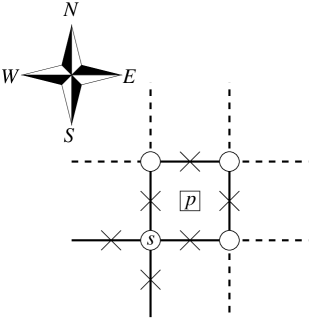
Figure 1: A single unit cell of the square array of wires, consisting of a single star $s$ and plaquette $p$. The dashed nearest-neigbor links belong to neighboring unit cells. The midpoint of each link hosts a quantum wire, represented by the symbol $\times$, aligned along the $z$-direction (out of the page). Any plaquette $p$ is surrounded by four quantum wires located at the four cardinal points $p^{\,}_{N}$, $p^{\,}_{W}$, $p^{\,}_{S}$, and $p^{\,}_{E}$, repectively. Similarly, any star $s$ is surrounded by four quantum wires located at the four cardinal points $s^{\,}_{N}$, $s^{\,}_{W}$, $s^{\,}_{S}$, and $s^{\,}_{E}$.

We now present a simple geometric prescription to aid in the determination of the existence (or lack thereof) of a Haldane set $\mathbb{H}$ for a two-dimensional array of quantum wires with some set of desired symmetries. This prescription capitalizes on the fact that we have chosen all $2N$ quantum wires to lie on the links of a square lattice. (In principle, this is not the only possible choice of lattice geometry, but it provides a simple way of counting degrees of freedom in any dimension, as we will see below and in Sec. III.) On a square lattice with $2N$ sites, there are $N$ “stars” (centered on the vertices of the lattice) and $N$ “plaquettes” (centered on the vertices of the dual lattice), assuming that periodic boundary conditions are imposed as in Fig. 1. If we associate the tunneling vectors $\mathcal{T}^{\,}_{s}$ and $\mathcal{T}^{\,}_{p}$ with each star $s$ and plaquette $p$, respectively, then we have a set of $2N$ tunneling vectors. Since there are $4MN$ gapless degrees of freedom in the array of decoupled quantum wires, we can obtain the necessary number $2MN$ of tunneling vectors by expanding this set to include $M$ “flavors” of tunneling vectors $\mathcal{T}^{(\texttt{j})}_{s}$ and $\mathcal{T}^{(\texttt{j})}_{p}$ for each star and plaquette, respectively. We label these flavors using a teletype index $\texttt{j}=1,\dots,M$. Imposing the Haldane criterion (11) on this set of tunneling vectors then yields the set of equations

$$\mathcal{T}^{(\texttt{j})\mathsf{T}}_{s}\ \mathcal{K}\ \mathcal{T}^{(\texttt{j}^{\prime})}_{s^{\prime}}=0\qquad\forall\ s,s^{\prime},\texttt{j},\texttt{j}^{\prime},$$ (12a)

$$\mathcal{T}^{(\texttt{j})\mathsf{T}}_{p}\ \mathcal{K}\ \mathcal{T}^{(\texttt{j}^{\prime})}_{p^{\prime}}=0\qquad\forall\ p,p^{\prime},\texttt{j},\texttt{j}^{\prime},$$ (12b)

$$\mathcal{T}^{(\texttt{j})\mathsf{T}}_{s}\ \mathcal{K}\ \mathcal{T}^{(\texttt{j}^{\prime})}_{p}=0\qquad\forall\ s,p,\texttt{j},\texttt{j}^{\prime}.$$ (12c)

If the above equations are satisfied, then the set of $2MN$ tunneling vectors is a Haldane set, and therefore capable of yielding a gapped phase in the strong-coupling limit.

(a)

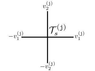
(b)

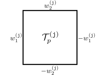
Figure 2: Pictorial representation of the tunneling vectors (13). The $2M$-dimensional integer-valued vectors $v^{(\texttt{j})}_{1,2}$ and $w^{(\texttt{j})}_{1,2}$ determine the linear combinations of bosonic fields in each wire that enter the cosine term associated with each star or plaquette, respectively.

We now turn to the problem of building $2MN$ tunneling vectors $\mathcal{T}^{(\texttt{j})}_{s}$ and $\mathcal{T}^{(\texttt{j})}_{p}$. Enumerating all solutions to this problem for all matrices $\mathcal{K}$ is beyond the scope of the present work. However, we will present below one way of constructing these tunneling vectors that builds in the minimal symmetries of charge and/or parity conservation [Eqs. (10)] and greatly reduces the number of equations that must be solved [relative to Eqs. (12), which contain an infinite number of linear equations in the thermodynamic limit $N\to\infty$ if no additional information is provided]. In particular, if we desire charge conservation [Eq. (10a)] to hold, we may define the tunneling vectors by their nonvanishing components

$$\begin{split}(\mathcal{T}^{(\texttt{j})}_{s})_{j,\alpha}&\,\raisebox{0.85pt}{.}\raisebox{2.85pt}{.}\!\!=\,v^{(\texttt{j})}_{1,\alpha}\,\left(\delta^{\,}_{j,s^{\,}_{E}}-\delta^{\,}_{j,s^{\,}_{W}}\right)\\ &\qquad\qquad+v^{(\texttt{j})}_{2,\alpha}\,\left(\delta^{\,}_{j,s^{\,}_{N}}-\delta^{\,}_{j,s^{\,}_{S}}\right),\end{split}$$ (13a)

$$\begin{split}(\mathcal{T}^{(\texttt{j})}_{p})_{j,\alpha}&\,\raisebox{0.85pt}{.}\raisebox{2.85pt}{.}\!\!=\,w^{(\texttt{j})}_{1,\alpha}\,\left(\delta^{\,}_{j,p^{\,}_{W}}-\delta^{\,}_{j,p^{\,}_{E}}\right)\\ &\qquad\qquad+w^{(\texttt{j})}_{2,\alpha}\,\left(\delta^{\,}_{j,p^{\,}_{N}}-\delta^{\,}_{j,p^{\,}_{S}}\right),\end{split}$$ (13b)

where we recall that $j=1,\dots,2N$ labels the quantum wires and $\alpha=1,\dots,2M$ labels the degrees of freedom within a wire. Here, $v^{(\texttt{j})}_{1}$, $v^{(\texttt{j})}_{2}$, $w^{(\texttt{j})}_{1}$, and $w^{(\texttt{j})}_{2}$ are arbitrary $2M$-dimensional integer vectors. The Kronecker deltas in the tunneling vector $\mathcal{T}^{\,}_{s}$ ensure that its nonzero entries are defined within the quantum wires $s^{\,}_{N},\dots,s^{\,}_{W}$ to the north, $\dots$, west of the vertex on which star $s$ is centered. The Kronecker deltas in $\mathcal{T}^{\,}_{p}$ select the quantum wires $p^{\,}_{N},\dots,p^{\,}_{W}$, which are defined similarly for the plaquette $p$ (see Fig. 1). With these definitions, one verifies that Eq. (10a) holds independently of the form of $v^{(\texttt{j})}_{1,2}$, $w^{(\texttt{j})}_{1,2}$, and the charge-vector $Q$ for a single wire.

Similarly, when we wish to impose number-parity conservation [Eq. (10b)], we may define for any $j=1,\dots,2N$ and any $\alpha=1,\dots,2M$

$$\begin{split}(\mathcal{T}^{(\texttt{j})}_{s})_{j,\alpha}&\,\raisebox{0.85pt}{.}\raisebox{2.85pt}{.}\!\!=\,v^{(\texttt{j})}_{1,\alpha}\,\left(\delta^{\,}_{j,s^{\,}_{E}}+\delta^{\,}_{j,s^{\,}_{W}}\right)\\ &\qquad\qquad+v^{(\texttt{j})}_{2,\alpha}\,\left(\delta^{\,}_{j,s^{\,}_{N}}+\delta^{\,}_{j,s^{\,}_{S}}\right),\end{split}$$ (14a)

$$\begin{split}(\mathcal{T}^{(\texttt{j})}_{p})_{j,\alpha}&\,\raisebox{0.85pt}{.}\raisebox{2.85pt}{.}\!\!=\,w^{(\texttt{j})}_{1,\alpha}\,\left(\delta^{\,}_{j,p^{\,}_{E}}+\delta^{\,}_{j,p^{\,}_{W}}\right)\\ &\qquad\qquad+w^{(\texttt{j})}_{2,\alpha}\,\left(\delta^{\,}_{j,p^{\,}_{N}}+\delta^{\,}_{j,p^{\,}_{S}}\right),\end{split}$$ (14b)

and verify that Eq. (10b) holds independently of the form of $v^{(\texttt{j})}_{1,2}$, $w^{(\texttt{j})}_{1,2}$, and $Q$.

Henceforth, we will focus on the charge-conserving tunneling vectors defined in Eqs. (13), as all general criteria discussed below have analogues for the parity-conserving tunneling vectors defined in Eqs. (14).

The charge-conserving tunneling vectors defined in Eqs. (13) are expressed in a convenient pictorial form in Fig. 2. From this pictorial representation, it is clear that any two distinct, adjacent stars (be they of the same flavor or different flavors) share a single wire between them. The same statement holds for plaquettes. However, adjacent stars and plaquettes share two wires between them, regardless of the flavor. Therefore, one can show that Eqs. (12) are satisfied if and only if

$$v^{(\texttt{j})\mathsf{T}}_{\mu}\,K\,v^{(\texttt{j}^{\prime})}_{\mu}=0,$$ (15a)

$$w^{(\texttt{j})\mathsf{T}}_{\mu}\,K\,w^{(\texttt{j}^{\prime})}_{\mu}=0,$$ (15b)

$$v^{(\texttt{j})\mathsf{T}}_{1}\,K\,w^{(\texttt{j}^{\prime})}_{2}-v^{(\texttt{j})\mathsf{T}}_{2}\,K\,w^{(\texttt{j}^{\prime})}_{1}=0,$$ (15c)

for all j and $\texttt{j}^{\prime}=1,\dots,M$ and $\mu=1,2$. Equations (15) are fundamental to our construction, as each solution to these equations for a given dimension $2M$ of the matrix $K$ may in principle describe a distinct gapped phase of matter.

Observe that Eqs. (15) are symmetric under $1\leftrightarrow 2$ and $\texttt{j}\leftrightarrow\texttt{j}^{\prime}$. Therefore, these criteria amount to a set of $5M(M+1)/2$ linear equations in $8M^{2}$ variables. This is important for two reasons. First, the number of equations does not scale with the number $2N$ of quantum wires in the array. This ensures that a single solution to these equations holds for any system size when periodic boundary conditions are imposed. Second, this set of equations is underconstrained for any $M$ (i.e., there are always more variables than equations). This means that for generic matrices $K$ of fixed dimension $2M$, there is in principle more than one solution to Eqs. (15).

We aim to construct gapped states of matter that have an isotropic low-energy description. Consequently, it is natural to demand that the tunneling vectors defined in Eqs. (13) and depicted in Fig. 2 are independent of direction. This can be achieved by imposing the additional constraints

$$v^{(\texttt{j})}_{1}=v^{(\texttt{j})}_{2}\,=\!\!\raisebox{0.85pt}{.}\raisebox{2.85pt}{.}\,v^{(\texttt{j})}$$ (16a)

and

$$w^{(\texttt{j})}_{1}=w^{(\texttt{j})}_{2}\,=\!\!\raisebox{0.85pt}{.}\raisebox{2.85pt}{.}\,w^{(\texttt{j})}.$$ (16b)

Note that Eq. (15c) is solved independently of the form of the $2M$-dimensional vectors $v^{(\texttt{j})}_{\mu}$ and $w^{(\texttt{j})}_{\mu}$ if Eqs. (16) hold. These constraints reduce the total number of variables contained in the tunneling vectors $\mathcal{T}^{\,}_{s}$ and $\mathcal{T}^{\,}_{p}$ from $8M^{2}$ to $4M^{2}$, and the number of nontrivial equations to $2M(M+1)/2$, i.e.,

$$v^{(\texttt{j})\mathsf{T}}\,K\,v^{(\texttt{j}^{\prime})}=0,$$ (17a)

$$w^{(\texttt{j})\mathsf{T}}\,K\,w^{(\texttt{j}^{\prime})}=0,$$ (17b)

which are merely rewritings of Eqs. (15a) and (15b). With this, we have arrived at the simplest incarnation of our construction. We will henceforth assume that Eqs. (17) hold for appropriate choices of the $2M$, $2M$-dimensional vectors $v^{(\texttt{j})}$ and $w^{(\texttt{j})}$. However, note that Eqs. (16) are sufficient but not necessary in order to produce a state of matter that has an isotropic low-energy description. We will therefore comment, as appropriate, on how our results below generalize to cases where $v^{(\texttt{j})}_{1}\neq v^{(\texttt{j})}_{2}$ and $w^{(\texttt{j})}_{1}\neq w^{(\texttt{j})}_{2}$.

II.3 Fractionalization

II.3.1 Change of basis

In this section, we outline how to use two-dimensional arrays of coupled quantum wires, like those described in the previous two sections, to study phases of matter with fractionalized excitations. To this end, let us assume that we have a Haldane set $\mathbb{H}$ containing $2MN$ tunneling vectors $\mathcal{T}^{(\texttt{j})}_{s}$ and $\mathcal{T}^{(\texttt{j})}_{p}$ with $\texttt{j}=1,\ldots,M$ defined by Eqs. (13) that satisfy (16) and the Haldane criterion (17). With these assumptions, the two-dimensional array of coupled quantum wires acquires a gap in the strong-coupling limit, yielding a three-dimensional gapped state of matter.

As discussed in the previous section, the phase of matter obtained in this way is a system of strongly-interacting fermions or bosons. However, for the purposes of studying fractionalization, it is convenient to work in a basis where the “fundamental” constituents of each wire are not fermions or bosons, but (possibly fractionalized) quasiparticles. This is achieved by making the change of basis

$$\tilde{\hat{\Phi}}(z)\,\raisebox{0.85pt}{.}\raisebox{2.85pt}{.}\!\!=\,\mathcal{W}^{-1}\,\hat{\Phi}(z),$$ (18a)

$$\tilde{\mathcal{V}}:=\mathcal{W}^{\mathsf{T}}\,\mathcal{V}\,\mathcal{W},$$ (18b)

$$\tilde{K}\,\raisebox{0.85pt}{.}\raisebox{2.85pt}{.}\!\!=\,W^{\mathsf{T}}\,K\,W,$$ (18c)

$$\tilde{Q}\,\raisebox{0.85pt}{.}\raisebox{2.85pt}{.}\!\!=\,W^{\mathsf{T}}\,Q,$$ (18d)

$$\tilde{\mathcal{T}}\,\raisebox{0.85pt}{.}\raisebox{2.85pt}{.}\!\!=\,\mathcal{W}^{-1}\,\mathcal{T},$$ (18e)

where

$$\mathcal{W}\,\raisebox{0.85pt}{.}\raisebox{2.85pt}{.}\!\!=\,\mathbbm{1}^{\,}_{2N}\otimes W,$$ (18f)

for some invertible $$2M\times 2M W$$ integer-valued matrix .

This change of variables has several virtues. First, $\tilde{K}$ remains symmetric and integer valued. Second, $\tilde{Q}$ remains integer valued. Third, this change of variables leaves the quantity $\mathcal{T}^{\mathsf{T}}\,\mathcal{K}\,\hat{\Phi}(z)$, which enters the argument of the cosine terms in Eq. (7), invariant, i.e.,

$$\tilde{\mathcal{T}}^{\mathsf{T}}\,\tilde{\mathcal{K}}\,\tilde{\hat{\Phi}}(z)=\mathcal{T}^{\mathsf{T}}\,\mathcal{K}\,\hat{\Phi}(z).$$ (19)

Thus, the linear transformation (18) does not change the character of the interaction itself, although it alters the tunneling vector $\mathcal{T}$ and the $4MN$-dimensional vector $\hat{\Phi}$ of bosonic fields. Furthermore, one verifies that the linear transformation (18) does not alter the compatibility criteria (15) or the quantity $\mathcal{Q}^{\mathsf{T}}\,\mathcal{T}$ that determines the presence or absence of charge or number-parity conservation.

Given the possibility of performing a change of basis of the form (18), we may now take a different approach. Instead of viewing the wire construction as a theory, with the Lagrangian (9), of scalar fields obeying the commutation relations (1d) with a $K$-matrix $K^{\,}_{\mathrm{f}}$ [Eq. (2)] for fermions or $K^{\,}_{\mathrm{b}}$ [Eq. (3)] for bosons, we may also view it as a theory, with the Lagrangian

$$\tilde{\hat{L}}\,\raisebox{0.85pt}{.}\raisebox{2.85pt}{.}\!\!=\,\tilde{\hat{L}}^{\,}_{0}+\tilde{\hat{L}}^{\,}_{\{\tilde{\mathcal{T}}\}},$$ (20)

of scalar fields obeying the new equal-time commutation relations

$$\left[\partial^{\,}_{z}\tilde{\hat{\phi}}^{\,}_{j,\alpha}(z),\tilde{\hat{\phi}}^{\,}_{j^{\prime},\alpha^{\prime}}(z^{\prime})\right] =\mathrm{i}\,2\pi\,\delta^{\,}_{jj^{\prime}}\,\tilde{K}^{-1}_{\alpha\alpha^{\prime}}\,\delta(z-z^{\prime}),$$ (21)

for $j,j^{\prime}=1,\dots,2N$ and $\alpha,\alpha^{\prime}=1,\cdots,2M$, which are neither fermionic nor bosonic in nature. We allow $\tilde{K}$ to be any symmetric, invertible, $2M\times 2M$ integer matrix, as long as it is related to $K^{\,}_{\mathrm{f}}$ or $K^{\,}_{\mathrm{b}}$ by a transformation of the form (18). Interactions between wires that yield a gapped state of matter can be constructed by following the procedures of the previous section. The $2M\,N$ integer tunneling vectors $\tilde{\mathcal{T}}^{(\texttt{j})}_{s}$ and $\tilde{\mathcal{T}}^{(\texttt{j})}_{p}$ obtained in this way form a Haldane set $\tilde{\mathbb{H}}$ related to the Haldane set $\mathbb{H}$ by the transformation (18). For reasons of simplicity that will become clear momentarily, we will concern ourselves in this paper primarily with the tunneling vectors $\tilde{\mathcal{T}}^{(\texttt{j})}_{s}$ and $\tilde{\mathcal{T}}^{(\texttt{j})}_{p}$ whose nonzero entries are equal to $\pm 1$. (Of course, nothing prevents us from also considering cases where this does not hold.) The counterparts $\mathcal{T}^{(\texttt{j})}_{s}$ and $\mathcal{T}^{(\texttt{j})}_{p}$ of these tunneling vectors under the transformation (18) generically have entries with magnitude larger than 1. This fact will be of importance to us now, as we turn to the issue of compactification.

II.3.2 Compactification, vertex operators, and fractional charges

Although the transformation (18) might appear innocuous, there is a fundamental difference between the theory with the Lagrangian $\tilde{\hat{L}}$ defined in Eq. (20) and the original fermionic or bosonic theory with the Lagrangian $\hat{L}$ defined in Eq. (9) when periodic boundary conditions are imposed in the $z$-direction (as we have assumed from the outset). In the latter theory, which is a theory of interacting electrons or bosons treated within bosonization, the traditional choice of compactification for the scalar fields $\hat{\phi}^{\,}_{j,\alpha}(z)$ with $j=1,\ldots,2N$ and $\alpha=1,\cdots,2M$ is

$$\hat{\phi}^{\,}_{j,\alpha}(z+L) \equiv\hat{\phi}^{\,}_{j,\alpha}(z)+2\pi\,n^{\,}_{\alpha},$$ (22)

for $n^{\,}_{\alpha}\in\mathbb{Z}^{2M}$. This choice ensures the single-valuedness of the fermionic or bosonic vertex operators (4) under $z\to z+L$, and, in turn, that of the Lagrangian $\hat{L}=\hat{L}^{\,}_{0}+\hat{L}^{\,}_{\{\mathcal{T}\}}$, as one can re-write $\hat{L}^{\,}_{\{\mathcal{T}\}}$ in terms of the correlated tunnelings (8), which reduce to products of these vertex operators. However, depending on the tunneling vectors $\mathcal{T}^{(\texttt{j})}_{s,p}$, there may be other, less stringent, compactifications of these scalar fields that also render the Lagrangian $\hat{L}$ single-valued under $z\to z+L$. The parsimonious course of action is to choose the “minimal” compactification, i.e., the smallest compactification radius that still maintains the single-valuedness of $\hat{L}$ under $z\to z+L$.

If the tunneling vectors $\mathcal{T}^{(\texttt{j})}_{s}$ and $\mathcal{T}^{(\texttt{j})}_{p}$ correspond to the tunneling vectors $\tilde{\mathcal{T}}^{(\texttt{j})}_{s}$ and $\tilde{\mathcal{T}}^{(\texttt{j})}_{p}$ under the transformation (18) whose only nonzero entries are equal to $\pm 1$, then there is a clear choice of minimal compactification. This choice can be obtained as follows. Working in the tilde basis, we can rewrite the interactions using the relation [analogous to (8)]

$$e^{-\mathrm{i}\,\tilde{\mathcal{T}}^{\mathsf{T}}\,\tilde{\mathcal{K}}\,\tilde{\hat{\Phi}}(z)}=\prod_{j=1}^{2N}\prod_{\alpha=1}^{2M}\left[\tilde{\hat{\psi}}^{{\dagger}}_{\mathrm{f,b};j,\alpha}(z)\right]^{\tilde{\mathcal{T}}^{\,}_{j,\alpha}},$$ (23a)

thereby implicitly defining a new set of fermionic or bosonic vertex operators,

$$\tilde{\hat{\psi}}^{{\dagger}}_{\mathrm{f,b};j,\alpha}(z)\,\raisebox{0.85pt}{.}\raisebox{2.85pt}{.}\!\!=\,\exp\left(-\mathrm{i}\,\sum_{\alpha^{\prime}=1}^{2M}\tilde{K}^{\,}_{\alpha\alpha^{\prime}}\,\tilde{\hat{\phi}}^{\,}_{j,\alpha^{\prime}}(z)\right).$$ (23b)

The minimal compactification is then obtained by demanding that this new set of vertex operators be single valued under $z\to z+L$. For any $j=1,\ldots,2N$ and $\alpha=1,\cdots,2M$, this is achieved by imposing the periodic boundary conditions

$$\tilde{\hat{\phi}}_{j,\alpha}(z+L) \equiv\tilde{\hat{\phi}}^{\,}_{j,\alpha}(z)+2\pi\,\tilde{K}^{-1}_{\alpha\alpha^{\prime}}\,n^{\,}_{\alpha^{\prime}},$$ (24)

for $n^{\,}_{\alpha}\in\mathbb{Z}^{2M}$. Here, there is an important difference with respect to Eq. (22). Because $\tilde{K}$ is an integer-valued matrix, $\tilde{K}^{-1}$ is generically a rational-valued matrix. The field $\tilde{\hat{\phi}}^{\,}_{j,\alpha}(z)$ is thus allowed to advance by rational (rather than integer) multiples of $2\pi$ when the coordinate $z$ is advanced through a full period $L$. This crucial distinction is what allows for the existence of fractionally-charged operators in the coupled wire array, as we now demonstrate.

Fractional quantum numbers appear in the wire construction because the compactification condition (24) allows for the existence of “quasiparticle” vertex operators

$$\hat{q}^{{\dagger}}_{j,\alpha}(z)\,\raisebox{0.85pt}{.}\raisebox{2.85pt}{.}\!\!=\,\exp\left(-\mathrm{i}\,\tilde{\hat{\phi}}^{\,}_{j,\alpha}(z)\right)$$ (25)

for any $j=1,\ldots,2N$ and $\alpha=1,\cdots,2M$ that are multivalued under the operation $z\mapsto z+L$. The fact that these vertex operators generically carry fractional charges can be seen by considering the transformed charge operator

$$\tilde{\hat{Q}}^{\,}_{j,\alpha}\,\raisebox{0.85pt}{.}\raisebox{2.85pt}{.}\!\!=\,\frac{\tilde{Q}^{\,}_{\alpha}}{2\pi}\,\sum_{\alpha^{\prime}=1}^{2M}\delta^{\,}_{\alpha\alpha^{\prime}}\int\limits^{L}_{0}\mathrm{d}z\ \partial^{\,}_{z}\,\tilde{\hat{\phi}}^{\,}_{j,\alpha^{\prime}}(z)$$ (26)

for any $j=1,\ldots,2N$ and $\alpha=1,\cdots,2M$. Its normalization is here chosen such that the fermionic or bosonic vertex operators defined in Eq. (23b) have charge $\tilde{Q}^{\,}_{\alpha}$. Indeed, for any $j,j^{\prime}=1,\ldots,2N$ and $\alpha,\alpha^{\prime}=1,\cdots,2M$, the equal-time commutator

$$\left[\tilde{\hat{Q}}^{\,}_{j,\alpha},\hat{q}^{{\dagger}}_{j^{\prime},\alpha^{\prime}}(z)\right]=\tilde{Q}^{\,}_{\alpha}\,\delta^{\,}_{jj^{\prime}}\,\tilde{K}^{-1}_{\alpha\alpha^{\prime}}\,\hat{q}^{{\dagger}}_{j^{\prime},\alpha^{\prime}}$$ (27)

indicates that, since $\tilde{K}^{-1}$ is generically a rational matrix, the quasiparticle operator $\hat{q}^{{\dagger}}_{j^{\prime},\alpha^{\prime}}$ generically has a rational charge. In particular, if $\tilde{Q}=Q$ under the transformation (18), and $\tilde{K}^{-1}$ has at least one rational entry with magnitude smaller than 1, the operator $\hat{q}^{{\dagger}}_{j^{\prime},\alpha^{\prime}}$ must then carry a fractional charge.

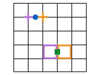
Figure 3: (Color online) Pictorial representation of star and plaquette excitations created by the operators (31). The filled blue circle represents an application of the vertex operator (31a) in the corresponding wire, while the purple and orange crosses represent defective stars hosting solitons of opposite signs. Similarly, the filled green square represents an application of the vertex operator (31b), and the purple and orange squares represent defective plaquettes hosting solitons of opposite signs.

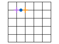
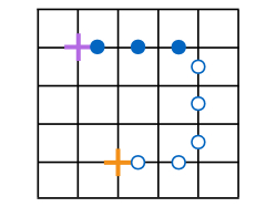
(a) (b)
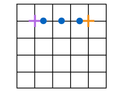
(c) (d)

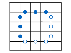
Figure 4: (Color online) Deconfinement of star defects within a plane. (a) A single application of the vertex operator (31a) (blue circle) creates a star defect (purple cross) and an anti-star defect (orange cross). (b) Applying a string of vertex operators (31a) moves a star defect by healing one while creating another. Consequently, it costs no extra energy to separate the two star defects. (c) To turn a corner, it may be necessary to heal a defect with an application of the inverse of the vertex operator (31a) in the appropriate wire (white circle). (d) When two star defects meet, they annihilate one another. A completely analogous description of plaquette defects also holds starting from the operators Eq. (31b).

II.3.3 Pointlike and linelike excitations

We now outline the relationship between the quasiparticle vertex operators defined in Eq. (25) and (possibly fractionalized) excitations in the array of coupled quantum wires. In the strong-coupling limit $U^{\,}_{\tilde{\mathcal{T}}}(z)\to\infty$, the compatibility criteria (15) ensure that the quantity

$$\tilde{\mathcal{T}}^{\mathsf{T}}\,\tilde{\mathcal{K}}\,\tilde{\hat{\Phi}}(z)+\alpha^{\,}_{\tilde{\mathcal{T}}}(z),$$ (28)

where $\tilde{\mathcal{T}}=\tilde{\mathcal{T}}^{(\texttt{j})}_{s}$ or $\tilde{\mathcal{T}}^{(\texttt{j})}_{p}$, is pinned to a classical minimum of the corresponding cosine potential in $\hat{L}^{\,}_{\{\tilde{\mathcal{T}}\}}$. Following Refs. Kane et al. (2002); Teo and Kane (2014) and subsequent works, we identify excitations in the coupled-wire theory with solitons that increment the “pinned field” $\tilde{\mathcal{T}}\,\tilde{\mathcal{K}}\,\tilde{\hat{\Phi}}(z)$ by an integer multiple of $2\pi$. These excitations can therefore be viewed as living on either the stars or the plaquettes of the square lattice, rather than within the wires themselves.

We now demonstrate that products of an appropriate number of quasiparticle vertex operators of the form (25) can be used to move the soliton defects to adjacent stars and plaquettes. To see this, we write out the pinned fields explicitly for all $MN$ tunneling vectors $\tilde{\mathcal{T}}^{(\texttt{j})}_{s}$ with $\texttt{j}=1,\ldots,M$ defined on the stars $s=1,\ldots,N$,

$$\tilde{\mathcal{T}}^{(\texttt{j})\mathsf{T}}_{s}\,\tilde{\mathcal{K}}\,\tilde{\hat{\Phi}}(z)=\sum_{\alpha,\alpha^{\prime}=1}^{2M}\tilde{v}^{(\texttt{j})}_{\alpha}\,\tilde{K}^{\,}_{\alpha\alpha^{\prime}}\,\left[\tilde{\hat{\phi}}^{\,}_{s^{\,}_{E},\alpha^{\prime}}(z)-\tilde{\hat{\phi}}^{\,}_{s^{\,}_{W},\alpha^{\prime}}(z)+\tilde{\hat{\phi}}^{\,}_{s^{\,}_{N},\alpha^{\prime}}(z)-\tilde{\hat{\phi}}^{\,}_{s^{\,}_{S},\alpha^{\prime}}(z)\right],$$ (29a)

and for all $$MN \tilde{\mathcal{T}}^{(\texttt{j})}_{p} \texttt{j}=1,\ldots,M p=1,\ldots,N$$ tunneling vectors with defined on the plaquettes ,

$$\tilde{\mathcal{T}}^{(\texttt{j})\mathsf{T}}_{p}\,\tilde{\mathcal{K}}\,\tilde{\hat{\Phi}}(z)=\sum_{\alpha,\alpha^{\prime}=1}^{2M}\tilde{w}^{(\texttt{j})}_{\alpha}\,\tilde{K}^{\,}_{\alpha\alpha^{\prime}}\left[\tilde{\hat{\phi}}_{p^{\,}_{W},\alpha^{\prime}}(z)-\tilde{\hat{\phi}}_{p^{\,}_{E},\alpha^{\prime}}(z)+\tilde{\hat{\phi}}^{\,}_{p^{\,}_{N},\alpha^{\prime}}(z)-\tilde{\hat{\phi}}^{\,}_{p^{\,}_{S},\alpha^{\prime}}(z)\right].$$ (29b)

For any star $s=1,\ldots,N$ or plaquette $p=1,\ldots,N$ from the square lattice and for any $\alpha,\beta=1,\ldots,2M$, observe that, by Eq. (21), the equal-time commutators

$$\left[\sum_{\alpha^{\prime}=1}^{2M}\tilde{K}^{\,}_{\alpha\alpha^{\prime}}\,\tilde{\hat{\phi}}^{\,}_{s^{\,}_{C},\alpha^{\prime}}(z),\partial^{\,}_{z^{\prime}}\tilde{\hat{\phi}}^{\,}_{s^{\,}_{C},\beta}(z^{\prime})\right]=\left[\sum_{\alpha^{\prime}=1}^{2M}\tilde{K}^{\,}_{\alpha\alpha^{\prime}}\,\tilde{\hat{\phi}}^{\,}_{p^{\,}_{C},\alpha^{\prime}}(z),\partial^{\,}_{z^{\prime}}\tilde{\hat{\phi}}^{\,}_{p^{\,}_{C},\beta}(z^{\prime})\right]=-\mathrm{i}\,2\pi\,\delta^{\,}_{\alpha\beta}\,\delta(z-z^{\prime})$$ (30)

hold. Here, the uppercase Latin index $C=N,W,S,E$ labels the four cardinal directions. Equation (30) indicates that the pair of fields $\partial^{\,}_{z}\tilde{\hat{\phi}}^{\,}_{s^{\,}_{C},\alpha}$ and $\partial^{\,}_{z}\tilde{\hat{\phi}}^{\,}_{p^{\,}_{C},\alpha}$ can be viewed, up to a multiplicative constant, as canonical conjugates to the pair of fields $\sum_{\alpha^{\prime}}\tilde{K}^{\,}_{\alpha\alpha^{\prime}}\,\tilde{\hat{\phi}}^{\,}_{s^{\,}_{C},\alpha^{\prime}}$ and $\sum_{\alpha^{\prime}}\tilde{K}^{\,}_{\alpha\alpha^{\prime}}\,\tilde{\hat{\phi}}^{\,}_{p^{\,}_{C},\alpha^{\prime}}(z)$ that enter the pair of pinned fields $\tilde{\mathcal{T}}^{(\texttt{j})\mathsf{T}}_{s}\,\tilde{\mathcal{K}}\,\tilde{\hat{\Phi}}$ and $\tilde{\mathcal{T}}^{(\texttt{j})\mathsf{T}}_{p}\,\tilde{\mathcal{K}}\,\tilde{\hat{\Phi}}$, respectively. Interpreted this way, Eqs. (30) suggest that, for any $\texttt{j}=1,\ldots,M$, $s^{\,}_{C}=s^{\,}_{N},s^{\,}_{W},s^{\,}_{S},s^{\,}_{E}$, and $p^{\,}_{C}=p^{\,}_{N},p^{\,}_{W},p^{\,}_{S},p^{\,}_{E}$, the operators

$$\hat{S}^{(\texttt{j}){\dagger}}_{s^{\,}_{C}}(z)\,\raisebox{0.85pt}{.}\raisebox{2.85pt}{.}\!\!=\,\exp\left(-\mathrm{i}\,\sum_{\alpha=1}^{2M}\tilde{v}^{(\texttt{j})}_{\alpha}\,\tilde{\hat{\phi}}^{\,}_{s^{\,}_{C},\alpha}(z)\right)$$ (31a)

and

$$\hat{P}^{(\texttt{j}){\dagger}}_{p^{\,}_{C}}(z)\,\raisebox{0.85pt}{.}\raisebox{2.85pt}{.}\!\!=\,\exp\left(-\mathrm{i}\,\sum_{\alpha=1}^{2M}\tilde{w}^{(\texttt{j})}_{\alpha}\,\tilde{\hat{\phi}}^{\,}_{p^{\,}_{C},\alpha}(z)\right)$$ (31b)

act on the pinned fields as [$|\tilde{v}^{(\texttt{j})}|^{2}$ denotes the magnitude squared of the vector $\tilde{v}^{(\texttt{j})}\in\mathbb{Z}^{2M}$]

$$\hat{S}^{(\texttt{j})}_{s^{\,}_{N}}(z^{\prime})\ \left[\tilde{\mathcal{T}}^{(\texttt{j})\mathsf{T}}_{s}\,\tilde{\mathcal{K}}\,\tilde{\hat{\Phi}}(z)\right]\ \hat{S}^{(\texttt{j}){\dagger}}_{s^{\,}_{N}}(z^{\prime})=\tilde{\mathcal{T}}^{(\texttt{j})\mathsf{T}}_{s}\,\tilde{\mathcal{K}}\,\tilde{\hat{\Phi}}(z)+2\pi\,|\tilde{v}^{(\texttt{j})}|^{2}\,\Theta(z-z^{\prime})+\text{constant},$$ (32a)

$$\hat{S}^{(\texttt{j})}_{s^{\,}_{W}}(z^{\prime})\ \left[\tilde{\mathcal{T}}^{(\texttt{j})\mathsf{T}}_{s}\,\tilde{\mathcal{K}}\,\tilde{\hat{\Phi}}(z)\right]\ \hat{S}^{(\texttt{j}){\dagger}}_{s^{\,}_{W}}(z^{\prime})=\tilde{\mathcal{T}}^{(\texttt{j})\mathsf{T}}_{s}\,\tilde{\mathcal{K}}\,\tilde{\hat{\Phi}}(z)-2\pi\,|\tilde{v}^{(\texttt{j})}|^{2}\,\Theta(z-z^{\prime})+\text{constant},$$ (32b)

$$\hat{S}^{(\texttt{j})}_{s^{\,}_{S}}(z^{\prime})\ \left[\tilde{\mathcal{T}}^{(\texttt{j})\mathsf{T}}_{s}\,\tilde{\mathcal{K}}\,\tilde{\hat{\Phi}}(z)\right]\ \hat{S}^{(\texttt{j}){\dagger}}_{s^{\,}_{S}}(z^{\prime})=\tilde{\mathcal{T}}^{(\texttt{j})\mathsf{T}}_{s}\,\tilde{\mathcal{K}}\,\tilde{\hat{\Phi}}(z)-2\pi\,|\tilde{v}^{(\texttt{j})}|^{2}\,\Theta(z-z^{\prime})+\text{constant},$$ (32c)

$$\hat{S}^{(\texttt{j})}_{s^{\,}_{E}}(z^{\prime})\ \left[\tilde{\mathcal{T}}^{(\texttt{j})\mathsf{T}}_{s}\,\tilde{\mathcal{K}}\,\tilde{\hat{\Phi}}(z)\right]\ \hat{S}^{(\texttt{j}){\dagger}}_{s^{\,}_{E}}(z^{\prime})=\tilde{\mathcal{T}}^{(\texttt{j})\mathsf{T}}_{s}\,\tilde{\mathcal{K}}\,\tilde{\hat{\Phi}}(z)+2\pi\,|\tilde{v}^{(\texttt{j})}|^{2}\,\Theta(z-z^{\prime})+\text{constant},$$ (32d)

and [$|\tilde{w}^{(\texttt{j})}|^{2}$ denotes the magnitude squared of the vector $\tilde{w}^{(\texttt{j})}\in\mathbb{Z}^{2M}$]

$$\hat{P}^{(\texttt{j})}_{p^{\,}_{N}}(z^{\prime})\ \left[\tilde{\mathcal{T}}^{(\texttt{j})\mathsf{T}}_{p}\,\tilde{\mathcal{K}}\,\tilde{\hat{\Phi}}(z)\right]\ \hat{P}^{(\texttt{j}){\dagger}}_{p^{\,}_{N}}(z^{\prime})=\tilde{\mathcal{T}}^{(\texttt{j})\mathsf{T}}_{p}\,\tilde{\mathcal{K}}\,\tilde{\hat{\Phi}}(z)+2\pi\,|\tilde{w}^{(\texttt{j})}|^{2}\,\Theta(z-z^{\prime})+\text{constant},$$ (33a)

$$\hat{P}^{(\texttt{j})}_{p^{\,}_{W}}(z^{\prime})\ \left[\tilde{\mathcal{T}}^{(\texttt{j})\mathsf{T}}_{p}\,\tilde{\mathcal{K}}\,\tilde{\hat{\Phi}}(z)\right]\ \hat{P}^{(\texttt{j}){\dagger}}_{p^{\,}_{W}}(z^{\prime})=\tilde{\mathcal{T}}^{(\texttt{j})\mathsf{T}}_{p}\,\tilde{\mathcal{K}}\,\tilde{\hat{\Phi}}(z)+2\pi\,|\tilde{w}^{(\texttt{j})}|^{2}\,\Theta(z-z^{\prime})+\text{constant},$$ (33b)

$$\hat{P}^{(\texttt{j})}_{p^{\,}_{S}}(z^{\prime})\ \left[\tilde{\mathcal{T}}^{(\texttt{j})\mathsf{T}}_{p}\,\tilde{\mathcal{K}}\,\tilde{\hat{\Phi}}(z)\right]\ \hat{P}^{(\texttt{j}){\dagger}}_{p^{\,}_{S}}(z^{\prime})=\tilde{\mathcal{T}}^{(\texttt{j})\mathsf{T}}_{p}\,\tilde{\mathcal{K}}\,\tilde{\hat{\Phi}}(z)-2\pi\,|\tilde{w}^{(\texttt{j})}|^{2}\,\Theta(z-z^{\prime})+\text{constant},$$ (33c)

$$\hat{P}^{(\texttt{j})}_{p^{\,}_{E}}(z^{\prime})\ \left[\tilde{\mathcal{T}}^{(\texttt{j})\mathsf{T}}_{p}\,\tilde{\mathcal{K}}\,\tilde{\hat{\Phi}}(z)\right]\ \hat{P}^{(\texttt{j}){\dagger}}_{p^{\,}_{E}}(z^{\prime})=\tilde{\mathcal{T}}^{(\texttt{j})\mathsf{T}}_{p}\,\tilde{\mathcal{K}}\,\tilde{\hat{\Phi}}(z)-2\pi\,|\tilde{w}^{(\texttt{j})}|^{2}\,\Theta(z-z^{\prime})+\text{constant},$$ (33d)

respectively. To verify Eqs. (32), one integrates both sides of the equalities entering Eq. (30) over the variable $z^{\prime}$ and uses the identity

$$\left(\frac{\mathrm{d}\Theta}{\mathrm{d}z}\right)(z)=\delta(z),$$ (34)

where $\Theta(z)$ is the Heaviside step function. If the underlying quantum wires in the theory are fermionic, the arbitrary integration constants above are identified with Klein factors that are necessary in order to ensure the anticommutation of fermionic vertex operators in different wires. If the underlying wires are bosonic, however, the integration constants can be set to zero.

Evidently, the operators $\hat{S}^{(\texttt{j}){\dagger}}_{s^{\,}_{C}}$ and $\hat{P}^{(\texttt{j}){\dagger}}_{p^{\,}_{C}}$ defined in Eqs. (31) create $2\pi$ solitons in the pinned fields $\tilde{\mathcal{T}}^{(\texttt{j})\mathsf{T}}_{s}\,\tilde{\mathcal{K}}\,\tilde{\hat{\Phi}}$ and $\tilde{\mathcal{T}}^{(\texttt{j})\mathsf{T}}_{p}\,\tilde{\mathcal{K}}\,\tilde{\hat{\Phi}}$, respectively. However, the link $s^{\,}_{C}$ on star $s$ is shared with the star $s^{\prime}$ adjacent to $s$ along the cardinal direction $C=N,W,S,E$, and, likewise, the link $p^{\,}_{C}$ on plaquette $p$ is shared with the plaquette $p^{\prime}$ adjacent to $p$ along the cardinal direction $C=N,W,S,E$. Therefore,

$$\hat{S}^{(\texttt{j})}_{s^{\,}_{N}}(z^{\prime})\ \left[\tilde{\mathcal{T}}^{(\texttt{j})\mathsf{T}}_{s^{\prime}}\,\tilde{\mathcal{K}}\,\tilde{\hat{\Phi}}(z)\right]\ \hat{S}^{(\texttt{j}){\dagger}}_{s^{\,}_{N}}(z^{\prime})=\tilde{\mathcal{T}}^{(\texttt{j})\mathsf{T}}_{s^{\prime}}\,\tilde{\mathcal{K}}\,\tilde{\hat{\Phi}}(z)-2\pi\,|\tilde{v}^{(\texttt{j})}|^{2}\,\Theta(z-z^{\prime})+\text{constant},$$ (35a)

$$\hat{S}^{(\texttt{j})}_{s^{\,}_{W}}(z^{\prime})\ \left[\tilde{\mathcal{T}}^{(\texttt{j})\mathsf{T}}_{s^{\prime}}\,\tilde{\mathcal{K}}\,\tilde{\hat{\Phi}}(z)\right]\ \hat{S}^{(\texttt{j}){\dagger}}_{s^{\,}_{W}}(z^{\prime})=\tilde{\mathcal{T}}^{(\texttt{j})\mathsf{T}}_{s^{\prime}}\,\tilde{\mathcal{K}}\,\tilde{\hat{\Phi}}(z)+2\pi\,|\tilde{v}^{(\texttt{j})}|^{2}\,\Theta(z-z^{\prime})+\text{constant},$$ (35b)

$$\hat{S}^{(\texttt{j})}_{s^{\,}_{S}}(z^{\prime})\ \left[\tilde{\mathcal{T}}^{(\texttt{j})\mathsf{T}}_{s^{\prime}}\,\tilde{\mathcal{K}}\,\tilde{\hat{\Phi}}(z)\right]\ \hat{S}^{(\texttt{j}){\dagger}}_{s^{\,}_{S}}(z^{\prime})=\tilde{\mathcal{T}}^{(\texttt{j})\mathsf{T}}_{s^{\prime}}\,\tilde{\mathcal{K}}\,\tilde{\hat{\Phi}}(z)+2\pi\,|\tilde{v}^{(\texttt{j})}|^{2}\,\Theta(z-z^{\prime})+\text{constant},$$ (35c)

$$\hat{S}^{(\texttt{j})}_{s^{\,}_{E}}(z^{\prime})\ \left[\tilde{\mathcal{T}}^{(\texttt{j})\mathsf{T}}_{s^{\prime}}\,\tilde{\mathcal{K}}\,\tilde{\hat{\Phi}}(z)\right]\ \hat{S}^{(\texttt{j}){\dagger}}_{s^{\,}_{E}}(z^{\prime})=\tilde{\mathcal{T}}^{(\texttt{j})\mathsf{T}}_{s^{\prime}}\,\tilde{\mathcal{K}}\,\tilde{\hat{\Phi}}(z)-2\pi\,|\tilde{v}^{(\texttt{j})}|^{2}\,\Theta(z-z^{\prime})+\text{constant},$$ (35d)

and

$$\hat{P}^{(\texttt{j})}_{p^{\,}_{N}}(z^{\prime})\ \left[\tilde{\mathcal{T}}^{(\texttt{j})\mathsf{T}}_{p^{\prime}}\,\tilde{\mathcal{K}}\,\tilde{\hat{\Phi}}(z)\right]\ \hat{P}^{(\texttt{j}){\dagger}}_{p^{\,}_{N}}(z^{\prime})=\tilde{\mathcal{T}}^{(\texttt{j})\mathsf{T}}_{p^{\prime}}\,\tilde{\mathcal{K}}\,\tilde{\hat{\Phi}}(z)-2\pi\,|\tilde{w}^{(\texttt{j})}|^{2}\,\Theta(z-z^{\prime})+\text{constant},$$ (36a)

$$\hat{P}^{(\texttt{j})}_{p^{\,}_{W}}(z^{\prime})\ \left[\tilde{\mathcal{T}}^{(\texttt{j})\mathsf{T}}_{p^{\prime}}\,\tilde{\mathcal{K}}\,\tilde{\hat{\Phi}}(z)\right]\ \hat{P}^{(\texttt{j}){\dagger}}_{p^{\,}_{W}}(z^{\prime})=\tilde{\mathcal{T}}^{(\texttt{j})\mathsf{T}}_{p^{\prime}}\,\tilde{\mathcal{K}}\,\tilde{\hat{\Phi}}(z)-2\pi\,|\tilde{w}^{(\texttt{j})}|^{2}\,\Theta(z-z^{\prime})+\text{constant},$$ (36b)

$$\hat{P}^{(\texttt{j})}_{p^{\,}_{S}}(z^{\prime})\ \left[\tilde{\mathcal{T}}^{(\texttt{j})\mathsf{T}}_{p^{\prime}}\,\tilde{\mathcal{K}}\,\tilde{\hat{\Phi}}(z)\right]\ \hat{P}^{(\texttt{j}){\dagger}}_{p^{\,}_{S}}(z^{\prime})=\tilde{\mathcal{T}}^{(\texttt{j})\mathsf{T}}_{p^{\prime}}\,\tilde{\mathcal{K}}\,\tilde{\hat{\Phi}}(z)+2\pi\,|\tilde{w}^{(\texttt{j})}|^{2}\,\Theta(z-z^{\prime})+\text{constant},$$ (36c)

$$\hat{P}^{(\texttt{j})}_{p^{\,}_{E}}(z^{\prime})\ \left[\tilde{\mathcal{T}}^{(\texttt{j})\mathsf{T}}_{p^{\prime}}\,\tilde{\mathcal{K}}\,\tilde{\hat{\Phi}}(z)\right]\ \hat{P}^{(\texttt{j}){\dagger}}_{p^{\,}_{E}}(z^{\prime})=\tilde{\mathcal{T}}^{(\texttt{j})\mathsf{T}}_{p^{\prime}}\,\tilde{\mathcal{K}}\,\tilde{\hat{\Phi}}(z)+2\pi\,|\tilde{w}^{(\texttt{j})}|^{2}\,\Theta(z-z^{\prime})+\text{constant},$$ (36d)

respectively. Note the sign difference with respect to Eqs. (32) and (33). This difference also stems from Fig. 2. Consequently, we interpret the operators $\hat{S}^{(\texttt{j}){\dagger}}_{s^{\,}_{C}}$ and $\hat{P}^{(\texttt{j}){\dagger}}_{p^{\,}_{C}}$ as creating a soliton-antisoliton pair straddling the links $s^{\,}_{C}=s^{\,}_{N},s^{\,}_{W},s^{\,}_{S},s^{\,}_{E}$ and $p^{\,}_{C}=p^{\,}_{N},p^{\,}_{W},p^{\,}_{S},p^{\,}_{E}$, respectively (see Fig. 3). By taking the derivative with respect to $z$ of Eqs. (32), (33), (35), and (36), we can interpret the operators $\hat{S}^{(\texttt{j}){\dagger}}_{s^{\,}_{C}}$ and $\hat{P}^{(\texttt{j}){\dagger}}_{p^{\,}_{C}}$ as creating a dipole in the soliton density across the links $s^{\,}_{C}=s^{\,}_{N},s^{\,}_{W},s^{\,}_{S},s^{\,}_{E}$ and $p^{\,}_{C}=p^{\,}_{N},p^{\,}_{W},p^{\,}_{S},p^{\,}_{E}$, respectively. Correspondingly, the annihilation vertex operators $\hat{S}^{(\texttt{j})}_{s^{\,}_{C}}$ and $\hat{P}^{(\texttt{j})}_{p^{\,}_{C}}$ reverse the orientations of these dipoles in the soliton density.

The defect and antidefect created by applying one of the operators $\hat{S}^{(\texttt{j}){\dagger}}_{s^{\,}_{C}}$ and $\hat{P}^{(\texttt{j}){\dagger}}_{p^{\,}_{C}}$ can be propagated away from one another in the $x$-$y$ plane by subsequent applications of the same operators on adjacent links, each of which “heal” one defect while creating another. An example of such a process is shown in Fig. 4. In the strong-coupling limit in which we work, this process does not generate any additional excitations, indicating that star and plaquette defects are deconfined in the $x$-$y$ plane. Furthermore, one can show that, in the same strong-coupling limit, these defects are also deconfined in the $z$-direction (see Appendix A for more details). Consequently, we conclude that the wire construction supports deconfined pointlike excitations, namely the star and plaquette defects. When these defects are separated from one another, there is a “string” of vertex operators connecting them. These strings are a crucial ingredient for determining the topological degeneracy, as we will see in the next section.

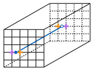
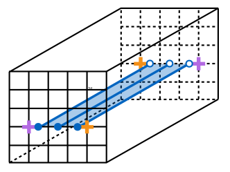
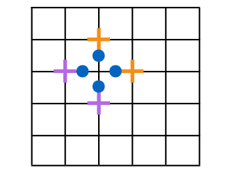
(a) (b) (c) (d)

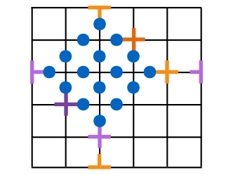
Figure 5: (color online) (a) A pair of linelike defects along the $z$ direction created by the operators (37). (b) Propagating one linelike defect away from the other using the operators (37) creates a membrane in the $x$-$z$ plane. (c) Growing a star membrane in the $x$-$y$ plane from the product of the operators (31a). (d) Membrane in the $x$-$y$ plane with defect lines on its boundaries. Darker purple or orange crosses indicate defective stars with a “double-strength” soliton, where two kinks of the same sign coexist in the same star.

The wire construction also supports deconfined linelike excitations. For any $\texttt{j}=1,\ldots,M$, pairs of linelike defects connecting the points $z^{\,}_{1}$ and $z^{\,}_{2}$ in a wire labelled by the link $s^{\,}_{C}=s^{\,}_{N},s^{\,}_{W},s^{\,}_{S},s^{\,}_{E}$ or $p^{\,}_{C}=p^{\,}_{N},p^{\,}_{W},p^{\,}_{S},p^{\,}_{E}$ can be created by the bi-local operators

$$\begin{split}\hat{S}^{(\texttt{j}){\dagger}}_{s^{\,}_{C}}(z^{\,}_{1},z^{\,}_{2})&\,\raisebox{0.85pt}{.}\raisebox{2.85pt}{.}\!\!=\,\hat{S}^{(\texttt{j}){\dagger}}_{s^{\,}_{C}}(z^{\,}_{2})\,\hat{S}^{(\texttt{j})\phantom{{\dagger}}}_{s^{\,}_{C}}(z^{\,}_{1})\\ &=\exp\bigg{(}-\mathrm{i}\,\sum_{\alpha=1}^{2M}\tilde{v}^{(\texttt{j})}_{\alpha}\int\limits^{z^{\,}_{2}}_{z^{\,}_{1}}\mathrm{d}z\ \partial^{\,}_{z}\tilde{\hat{\phi}}^{\,}_{s^{\,}_{C},\alpha}(z)\bigg{)},\end{split}$$ (37a)

$$\begin{split}\hat{P}^{(\texttt{j}){\dagger}}_{p^{\,}_{C}}(z^{\,}_{1},z^{\,}_{2})&\,\raisebox{0.85pt}{.}\raisebox{2.85pt}{.}\!\!=\,\hat{P}^{(\texttt{j}){\dagger}}_{p^{\,}_{C}}(z^{\,}_{2})\,\hat{P}^{(\texttt{j})\phantom{{\dagger}}}_{p^{\,}_{C}}(z^{\,}_{1})\\ &=\exp\bigg{(}-\mathrm{i}\,\sum_{\alpha=1}^{2M}\tilde{w}^{(\texttt{j})}_{\alpha}\int\limits^{z^{\,}_{2}}_{z^{\,}_{1}}\mathrm{d}z\ \partial^{\,}_{z}\tilde{\hat{\phi}}^{\,}_{p^{\,}_{C},\alpha}(z)\bigg{)},\end{split}$$ (37b)

a pictorial example of which is depicted in Fig. 5(a). Similarly to the propagation of star and plaquette defects outlined in the previous paragraph, applying a string of the above operators creates a membrane with linelike defects at its boundaries in the $z$-$x$ and $y$-$z$ planes as is illustrated Fig. 5(b).

The membranes created by applying strings of the operators defined in Eqs. (37) necessarily extend in the $x$-$z$ or $y$-$z$ planes. Membranes extending in the $x$-$y$ plane can also be created by applying the operators defined in Eqs. (31) over a membrane as opposed to a string, as in Fig. 5(c-d). As with the $x$-$z$ and $y$-$z$ membranes, the boundary of an $x$-$y$ membrane supports linelike defects.

It is important to note that the strings and membranes connecting pairs of pointlike and linelike defects, respectively, may fluctuate in all directions. The origin of these fluctuations lies in the existence of a discrete gauge symmetry that can be formulated explicitly in the strong coupling limit $|U^{\,}_{\tilde{\mathcal{T}}}|\to\infty$. (We elaborate on the physical meaning of this limit in the next section.) We carry out this formulation in Appendix B. Strings and membranes that fluctuate in this way are familiar from the toric code and other string-net models.

II.3.4 Energetics of pointlike and linelike defects

At this stage, a brief comment is in order regarding the energetics of the pointlike and linelike defects defined in Sec. II.3.3. It is misleading to compute the energy cost of such a defect in the strong-coupling limit $|U^{\,}_{\tilde{\mathcal{T}}}|\to\infty$, as in this limit, the perfectly sharp solitons created by the operators $\hat{S}^{(\texttt{j}){\dagger}}_{s^{\,}_{C}}$ and $\hat{P}^{(\texttt{j}){\dagger}}_{p^{\,}_{C}}$ [recall Eqs. (32) and (33)] cost no energy from the point of view of the cosine terms (7). This is simply because these solitons increment the argument of a cosine term abruptly at some $z$ by an integer multiple of $2\pi$, which amounts to a discontinuous jump between exact minima of the cosine potential. However, the presence of an infinitesimal kinetic term of the form (1a) gives a finite stiffness $\kappa$ to the pinned field. In this case, the optimal soliton profile is no longer the perfectly sharp one generated by the operators $\hat{S}^{(\texttt{j}){\dagger}}_{s^{\,}_{C}}$ and $\hat{P}^{(\texttt{j}){\dagger}}_{p^{\,}_{C}}$, but a slightly deformed one where the interpolation between minima of the cosine potential is smeared over a length scale $\xi$.

Suppose that this optimal soliton profile is known. Then, it is possible to redefine the operators $\hat{S}^{(\texttt{j}){\dagger}}_{s^{\,}_{C}}$ and $\hat{P}^{(\texttt{j}){\dagger}}_{p^{\,}_{C}}$ in such a way that they act on the pinned fields as in Eqs. (32) and (33), but now with the perfectly sharp soliton profile replaced by the optimal one. [Note that this redefinition can be done without altering the fundamental commutation relations (21) on length scales longer than $\xi$.] The energy cost of such an optimal soliton is composed of two contributions: one from the cosine potential (assumed to be large) and one from the stiffness (assumed to be small but finite).

Once the finite energy cost of a single soliton has been determined, it is readily seen that the stringlike and membranelike operators defined in Sec. II.3.3 cannot dissociate into smaller pointlike or linelike operators without an energy cost that is extensive in the number of vertex operators used to build the string or membrane. For example, if one tries to pull apart the string of vertex operators shown in Fig. 4(b) so that all operators in the string are disconnected, one necessarily increases the energy by an amount proportional to the number of vertex operators in the chain. This is because each application of a vertex operator in the latter scenario costs energy due to two cosine terms (in addition to the stiffness). In contrast, when the vertex operators form a string, the only energy cost due to the cosine terms occurs at the two ends of the string.

Finally, one might be concerned that the energetic effects discussed above could lead to confinement of star and plaquette defects. Indeed, if the stiffness $\kappa$ is finite, then strings of vertex operators like the ones depicted in Fig. 4 necessarily cost an energy proportional to their length. In fact, there is a direct parallel here with the confinement-deconfinement transition in the toric code Kitaev (2003). In that case, two star defects (say) are connected by a string of flipped spins. Thus, there is a measurable trail of magnetization that connects the two defects. However, in the absence of an external magnetic field, there is no energy cost associated with such a string. The presence of a sufficiently large external field leads to confinement, but, below a critical field strength, entropic effects are sufficient to deconfine the defects. In our system, the role of the external magnetic field is played by the kinetic term, which is the origin of the stiffness $\kappa$.

Thus, provided that the stiffness $\kappa\ll|U^{\,}_{\tilde{\mathcal{T}}}|$, we expect that defects in our model are deconfined because entropic effects favor deconfinement, as is the case in the toric code. When $\kappa$ reaches some critical value, however, the defects become confined.

II.3.5 Statistics of pointlike and linelike defects

We have enumerated the pointlike and linelike excitations for a class of two-dimensional arrays of coupled quantum wires by showing how to use vertex operators to build open stringlike and open membranelike operators supporting these defects on their boundaries. The statistics of these excitations are readily accessible within the wire formalism, as we now explain.

In principle, there are several types of statistics to consider. The first type, that of different types of pointlike excitations, must be trivial in three dimensions by homotopy arguments. Leinaas and Myrheim (1977) (Essentially, such arguments hinge on the fact that any loop that one particle makes around another in three dimensions can be deformed to a point without passing through the other particle.)

The second type, that of pointlike and linelike excitations, can be nontrivial in three dimensions, and will be computed below for the class of models defined here.

The third type of statistics, that between linelike excitations, can also be nontrivial in three dimensions, but can be shown to be trivial in the present class of models.

Let us first examine the mutual statistics between pointlike and linelike defects. Using the identity

$$e^{\hat{A}}\,e^{\hat{B}}=e^{\hat{B}}\,e^{\hat{A}}\ e^{[\hat{A},\hat{B}]}$$ (38)

which follows from the Baker-Campbell-Hausdorff lemma whenever $[\hat{A},\hat{B}]$ is a $c$-number, one can show from Eq. (21) that, for any $\texttt{j},\texttt{j}^{\prime}=1,\ldots,N$ and for any $s^{\,}_{C},s^{\,}_{C^{\prime}}=s^{\,}_{N},s^{\,}_{W},s^{\,}_{S},s^{\,}_{E}$ or $p^{\,}_{C},p^{\,}_{C^{\prime}}=p^{\,}_{N},p^{\,}_{W},p^{\,}_{S},p^{\,}_{E}$,

$$\begin{split}&\hat{S}^{(\texttt{j}){\dagger}}_{s^{\,}_{C}}(z)\,\hat{P}^{(\texttt{j}^{\prime}){\dagger}}_{p^{\,}_{C^{\prime}}}(z^{\prime}_{1},z^{\prime}_{2})\\ &\qquad=\hat{P}^{(\texttt{j}^{\prime}){\dagger}}_{p^{\,}_{C^{\prime}}}(z^{\prime}_{1},z^{\prime}_{2})\,\hat{S}^{(\texttt{j}){\dagger}}_{s^{\,}_{C}}(z)\,e^{+\mathrm{i}\,2\pi\,\tilde{v}^{(\texttt{j})\mathsf{T}}\,\tilde{K}^{-1}\,\tilde{w}^{(\texttt{j}^{\prime})}\,\delta^{\,}_{s^{\,}_{C},p^{\,}_{C^{\prime}}}},\end{split}$$ (39a)

$$\begin{split}&\hat{S}^{(\texttt{j}){\dagger}}_{s^{\,}_{C}}(z^{\prime}_{1},z^{\prime}_{2})\,\hat{P}^{(\texttt{j}^{\prime}){\dagger}}_{p^{\,}_{C^{\prime}}}(z)\\ &\qquad=\hat{P}^{(\texttt{j}^{\prime}){\dagger}}_{p^{\,}_{C^{\prime}}}(z)\,\hat{S}^{(\texttt{j}){\dagger}}_{s^{\,}_{C}}(z^{\prime}_{1},z^{\prime}_{2})\,e^{-\mathrm{i}\,2\pi\,\tilde{v}^{(\texttt{j})\mathsf{T}}\,\tilde{K}^{-1}\,\tilde{w}^{(\texttt{j}^{\prime})}\,\delta^{\,}_{s^{\,}_{C},p^{\,}_{C^{\prime}}}},\end{split}$$ (39b)

whenever $z^{\prime}_{1}<z<z^{\prime}_{2}$.

Figure 6: (Color online) Pictorial representation for braiding a pointlike plaquette defect [defined in Eq. (31b)] around a linelike star defect along the $z$-direction [defined in Eq. (37a)]. The green colored loop represents the worldline during adiabatic braiding of one end of an open plaquette string, say the plaquette counterpart to the open string depicted in Fig. 4(c). By choice, the world line encloses the rightmost boundary of the star membrane in Fig. 5(b).

With these relations in hand, one can readily compute the algebra of the membrane and string operators that are used to create and propagate pointlike and linelike defect-antidefect pairs. As discussed in Ref. Lin and Levin (2015), this algebra determines the phase obtained by winding a pointlike excitation around a linelike excitation. The computation of this phase is cumbersome to write down, but nevertheless quite straightforward—a convenient way to see this comes from the pictorial representation of such a braiding process (see Fig. 6 for an example). From this pictorial representation, one sees immediately that the membrane and string operators associated with stars commute with one another (and likewise for plaquettes), as they never intersect in a wire. However, membranes associated with star defects and strings associated with plaquette defects (and vice versa) always intersect with one another during a braiding process. The total phase arising from commuting one operator past the other can then be read off from the picture using Eqs. (39). We find that the statistical phase obtained by braiding a pointlike plaquette defect around a linelike star defect is given by

$$\frac{\theta^{\,}_{\texttt{j}\texttt{j}^{\prime}}}{2\pi}=\tilde{v}^{(\texttt{j})\mathsf{T}}\,\tilde{K}^{-1}\,\tilde{w}^{(\texttt{j}^{\prime})}=\tilde{w}^{(\texttt{j}^{\prime})\mathsf{T}}\,\tilde{K}^{-1}\tilde{v}^{(\texttt{j})}$$ (40)

for any $\texttt{j},\texttt{j}^{\prime}=1,\ldots,M$, where the second equality follows from the fact that $\tilde{K}^{-1}$ is a symmetric matrix.

At this point, we remark that, although the construction of operators undertaken in this section and in the previous section has assumed that $\tilde{v}^{(\texttt{j})}_{1}=\tilde{v}^{(\texttt{j})}_{2}=\tilde{v}^{(\texttt{j})}$ and $\tilde{w}^{(\texttt{j})}_{1}=\tilde{w}^{(\texttt{j})}_{2}=\tilde{w}^{(\texttt{j})}$, this construction proceeds with only minor modifications in the more general case $\tilde{v}^{(\texttt{j})}_{1}\neq\tilde{v}^{(\texttt{j})}_{2}$ and $\tilde{w}^{(\texttt{j})}_{1}\neq\tilde{w}^{(\texttt{j})}_{2}$. However, in the latter case, one finds that the statistical angle must obey

$$\frac{\theta_{\texttt{j}\texttt{j}^{\prime}}}{2\pi}=\tilde{v}^{(\texttt{j})\mathsf{T}}_{1}\,\tilde{K}^{-1}\,\tilde{w}^{(\texttt{j}^{\prime})}_{2}\overset{!}{=}\tilde{v}^{(\texttt{j})\mathsf{T}}_{2}\,\tilde{K}^{-1}\,\tilde{w}^{(\texttt{j}^{\prime})}_{1}$$ (41)

for any $\texttt{j},\texttt{j}^{\prime}=1,\ldots,M$. The second equality in Eq. (41) must be imposed as a consistency condition. Otherwise, the statistical angle $\theta^{\,}_{\texttt{j}\texttt{j}^{\prime}}$ would depend on whether the string and membrane operators used to compute the statistics intersected on vertical or horizontal bonds. (See, e.g., Fig. 6, where the string and membrane intersect on a horizontal bond.) Thus, we must demand that Eq. (41) holds, as otherwise the low-energy description of the theory would be anisotropic.

We close this section by outlining the reason why the line-line statistics in this class of models is trivial. The statistical phase describing the line-line statistics is computed using membrane surfaces arranged as in Fig. 7. From this, it is clear that the relevant operator product to consider is of the form

$$\hat{S}^{(\texttt{j}){\dagger}}_{s^{\,}_{C}}(z^{\,}_{1},z^{\,}_{2})\,\hat{P}^{(\texttt{j}^{\prime}){\dagger}}_{p^{\,}_{C^{\prime}}}(z^{\prime}_{1},z^{\prime}_{2})=\hat{S}^{(\texttt{j}){\dagger}}_{s^{\,}_{C}}(z^{\,}_{1},z^{\,}_{2})\,\hat{P}^{(\texttt{j}^{\prime}){\dagger}}_{p^{\,}_{C^{\prime}}}(z^{\prime}_{1},z^{\prime}_{2})\,\exp\!\left(\!-\mathrm{i}\!\sum_{\alpha,\beta=1}^{2M}\tilde{v}^{(\texttt{j})}_{\alpha}\tilde{w}^{(\texttt{j}^{\prime})}_{\beta}\int\limits^{z^{\,}_{2}}_{z^{\,}_{1}}\!\mathrm{d}z\int\limits^{z^{\prime}_{2}}_{z^{\prime}_{1}}\!\mathrm{d}z^{\prime}\left[\partial^{\,}_{z}\tilde{\hat{\phi}}^{\,}_{s^{\,}_{C},\alpha}(z),\partial^{\,}_{z^{\prime}}\tilde{\hat{\phi}}^{\,}_{p^{\,}_{C^{\prime}},\beta}(z^{\prime})\right]\right)$$ (42)

for any $\texttt{j}=1,\ldots,M$, $s^{\,}_{C}=s^{\,}_{N},s^{\,}_{W},s^{\,}_{S},s^{\,}_{E}$, and $p^{\,}_{C^{\prime}}=p^{\,}_{N},p^{\,}_{W},p^{\,}_{S},p^{\,}_{E}$, where it is assumed that the interval $[z^{\,}_{1},z^{\,}_{2}]\subset[z^{\prime}_{1},z^{\prime}_{2}]$ or vice versa. However, by differentiating Eq. (21) with respect to $z^{\prime}$, one sees that the commutator in the exponential is proportional to the derivative of a delta function. Integrated over both $z$ and $z^{\prime}$, this yields zero for the statistical angle between two lines. In a similar manner, one can show that the three-line statistics (c.f. Ref. Lin and Levin (2015)) is trivial in this class of models.

This discussion of the excitations of the coupled-wire construction provides sufficient information to determine the minimal topological ground-state degeneracy of the theory, as we now show.

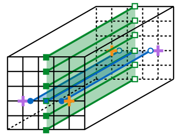
Figure 7: (Color online) Pictorial representation of braiding a star line and a plaquette line. Because periodic boundary conditions are imposed in all directions and because we choose to represent the worldsheet induced by the adiabatic evolution of plaquette linelike defects by the green membrane that extends across the width of the lattice in the $y$ direction, this world sheet forms a cylinder with its symmetry axis parallel to the $z$ direction. By choice, this cylinder encircles the star-type line that defines the rightmost boundary of the blue membrane. The algebra encoded by Eq. (42) implies that such a braiding yields no overall statistical phase.

II.3.6 Topological ground-state degeneracy

The theory defined in Eq. (20) by the Lagrangian $\tilde{\hat{L}}=\tilde{\hat{L}}^{\,}_{0}+\tilde{\hat{L}}^{\,}_{\{\tilde{\mathcal{T}}\}}$ generically exhibits a ground-state degeneracy when defined on the three-torus obtained by imposing periodic boundary conditions in the $x$-, $y$-, and $z$-directions. We present an argument as to why this is the case.

First, recall that, when periodic boundary conditions are imposed in the $x$- and $y$-directions, for a square lattice with $2N$ links, there are $4\,M\,N$ degrees of freedom ($2\,M$ per wire). There are also $M\,N$ star and $M\,N$ plaquette terms entering the interaction $\tilde{\hat{H}}^{\,}_{\mathrm{int}}\equiv-\tilde{\hat{L}}^{\,}_{\{\tilde{\mathcal{T}}\}}$ defined in Eq. (20), each of which gaps out two of these degrees of freedom. The number of star and plaquette operators in $\tilde{\hat{L}}^{\,}_{\{\tilde{\mathcal{T}}\}}$ is therefore sufficient to gap out the bulk of the wire array, as mentioned above.

It is shown in Appendix B for $M=1$ with the choice made in Sec. II.4 for the integer-valued vectors $\tilde{v}$ and $\tilde{w}$ that there are $4\,N$ local vertex operators, namely two per star $s$ and two per plaquette $p$, that commute with the interaction $\tilde{\hat{H}}^{\,}_{\mathrm{int}}\equiv-\tilde{\hat{L}}^{\,}_{\{\tilde{\mathcal{T}}\}}$. The proof in Appendix B readily generalizes to arbitrary $M=1,2,\dots$ and the integer-valued vectors $\tilde{v}^{(\texttt{j})}$ and $\tilde{w}^{(\texttt{j})}$ with $\texttt{j}=1,\dots,M$ entering Fig. 2. This local gauge symmetry implies that all the cosines entering the interaction $\tilde{\hat{H}}^{\,}_{\mathrm{int}}\equiv-\tilde{\hat{L}}^{\,}_{\{\tilde{\mathcal{T}}\}}$ commute pairwise. This local gauge symmetry also implies that deconfining the pointlike and stringlike defects costs no energy in the strong coupling limit where the full Hamiltonian $\tilde{\hat{H}}$ defined by Eq. (20) reduces to $\tilde{\hat{H}}^{\,}_{\mathrm{int}}\equiv-\tilde{\hat{L}}^{\,}_{\{\tilde{\mathcal{T}}\}}$. Hence, the strong coupling limit $\tilde{\hat{H}}=\tilde{\hat{H}}^{\,}_{\mathrm{int}}$ is very singular since the gap induced by the cosines from the Haldane set $\tilde{\mathbb{H}}$ collapses. (As argued in Sec. II.3.4, including an infinitesimal kinetic term rectifies this singularity and yields a finite energy cost for the creation of star and plaquette defects.)

Now, for any given coordinate $0\leq z<L$ along a wire, there are $2\,M$ global constraints obeyed by the generators of this local gauge symmetry. Indeed,

$$\prod_{p\in\mathcal{P}}e^{\mathrm{i}\,\tilde{\mathcal{T}}^{(\texttt{j})\mathsf{T}}_{p}\,\tilde{\mathcal{K}}\,\tilde{\hat{\Phi}}(z)} =1$$ (43a)

and

$$\prod_{s\in\mathcal{S}}e^{\mathrm{i}\,\tilde{\mathcal{T}}^{(\texttt{j})\mathsf{T}}_{s}\,\tilde{\mathcal{K}}\,\tilde{\hat{\Phi}}(z)}=1,$$ (43b)

hold for all $\texttt{j}=1,\dots M$ and all $z\in[0,L)$. Here, $\mathcal{P}$ and $\mathcal{S}$ are the sets of all plaquettes and stars in the square lattice, respectively. These constraints result from the fact that

$$\sum_{p\in\mathcal{P}}\tilde{\mathcal{T}}^{(\texttt{j})}_{p}=\sum_{s\in\mathcal{S}}\tilde{\mathcal{T}}^{(\texttt{j})}_{s}=0$$ (44)

for each $\texttt{j}=1,\dots M$.

The $2\,M$ constraints (43) are inherently nonlocal. Removing any of the $\tilde{\mathcal{T}}^{(\texttt{j})}_{s}$ or $\tilde{\mathcal{T}}^{(\texttt{j})}_{p}$ for fixed j from the set $\tilde{\mathbb{H}}$ invalidates the constraints (43). If the number of independent commuting operators that commute with $\tilde{\hat{H}}^{\,}_{\mathrm{int}}\equiv-\tilde{\hat{L}}^{\,}_{\{\tilde{\mathcal{T}}\}}$ defined in Eq. (20) is to match the number of degrees of freedom, the constraints (43) necessitate the existence of additional nonlocal operators that commute with $\tilde{\hat{H}}^{\,}_{\mathrm{int}}$. It turns out that such operators exist and that the ground-state degeneracy is related to the representation of the algebra of these nonlocal operators that has the smallest dimensionality. We will now enumerate these operators, compute their algebra, and deduce from this algebra the ground state degeneracy of the wire construction. One important result will be that there is a unique (i.e., non-degenerate) ground state if $|\det\,\tilde{K}|=1$, a result that is familiar from Abelian Chern-Simons theories in (2+1) dimensions Wen (1989); Wen and Niu (1990); Wen (1991); Wen and Zee (1992) and reappears in the present (3+1)-dimensional context.

We are going to define two types of non-local operators out of the local operators (31) and the bi-local operators (37).

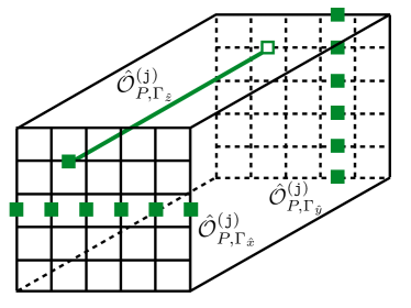
Figure 8: (Color online) Pictorial representation of the plaquette-type string operators defined in Eqs. (45). The star-type string operators are defined similarly.

First, for any $\texttt{j}=1,\cdots,M$, any cardinal directions $C,C^{\prime}=N,W,S,E$, and any $0\leq z<L$, we define the non-local string operators

$$\hat{\mathcal{O}}^{(\texttt{j})}_{S,\Gamma^{\,}_{x}}(z)\,\raisebox{0.85pt}{.}\raisebox{2.85pt}{.}\!\!=\,\prod_{s^{\,}_{C}\in\Gamma^{\,}_{x}}\hat{S}^{(\texttt{j}){\dagger}}_{s^{\,}_{C}}(z),$$ (45a)

$$\hat{\mathcal{O}}^{(\texttt{j})}_{S,\Gamma^{\,}_{y}}(z)\,\raisebox{0.85pt}{.}\raisebox{2.85pt}{.}\!\!=\,\prod_{s^{\,}_{C}\in\Gamma^{\,}_{y}}\hat{S}^{(\texttt{j}){\dagger}}_{s^{\,}_{C}}(z),$$ (45b)

$$\hat{\mathcal{O}}^{(\texttt{j})}_{S,\Gamma^{\,}_{z}}\,\raisebox{0.85pt}{.}\raisebox{2.85pt}{.}\!\!=\,\hat{S}^{(\texttt{j}){\dagger}}_{s^{\,}_{C}}(0,L),$$ (45c)

and

$$\hat{\mathcal{O}}^{(\texttt{j})}_{P,\Gamma^{\,}_{\hat{x}}}(z)\,\raisebox{0.85pt}{.}\raisebox{2.85pt}{.}\!\!=\,\prod_{p^{\,}_{C}\in\Gamma^{\,}_{\hat{x}}}\hat{P}^{(\texttt{j}){\dagger}}_{p^{\,}_{C}}(z),$$ (45d)

$$\hat{\mathcal{O}}^{(\texttt{j})}_{P,\Gamma^{\,}_{\hat{y}}}(z)\,\raisebox{0.85pt}{.}\raisebox{2.85pt}{.}\!\!=\,\prod_{p^{\,}_{C}\in\Gamma^{\,}_{\hat{y}}}\hat{P}^{(\texttt{j}){\dagger}}_{p^{\,}_{C}}(z),$$ (45e)

$$\hat{\mathcal{O}}^{(\texttt{j})}_{P,\Gamma^{\,}_{\hat{z}}}\,\raisebox{0.85pt}{.}\raisebox{2.85pt}{.}\!\!=\,\hat{P}^{(\texttt{j}){\dagger}}_{p^{\,}_{C^{\prime}}}(0,L).$$ (45f)

Here, $\Gamma^{\,}_{x}$ is a non-contractible, directed, closed path traversing the entire square lattice along the direction $x$, while $\Gamma^{\,}_{\hat{x}}$ is a non-contractible, directed, closed path traversing the entire dual lattice along the direction $\hat{x}$. [A directed path consists of the set of links, either $s^{\,}_{C}\in\Gamma^{\,}_{x}$ or $p^{\,}_{C}\in\Gamma^{\,}_{\hat{x}}$, to be traversed according to the ordering in the product of vertex operators on the right-hand sides of Eqs. (45a) and (45b), respectively.] Similarly, the non-contractible, directed, closed paths $\Gamma^{\,}_{y}$ and $\Gamma^{\,}_{\hat{y}}$ traverse the square lattice along the $y$- and $\hat{y}$-directions, respectively. Finally, $\Gamma^{\,}_{z}$ and $\Gamma^{\,}_{\hat{z}}$ are non-contractible closed paths traversing a wire in the $z$ and $\hat{z}$ directions, respectively. On the right-hand sides of Eqs. (45c) and (45f), the choice of the link $s^{\,}_{C}=s^{\,}_{N},s^{\,}_{W},s^{\,}_{S},s^{\,}_{E}$ and $p^{\,}_{C^{\prime}}=p^{\,}_{N},p^{\,}_{W},p^{\,}_{S},p^{\,}_{E}$, respectively, is of no consequence for the purposes of computing the topological degeneracy (see below). For a pictorial representation of these string operators, see Fig. 8. These operators can be interpreted as describing processes in which particle-antiparticle pairs of different types of star or plaquette defects are created, and where the particle propagates along a non-contractible loop that encircles the entire torus before annihilating with its antiparticle.

(a)

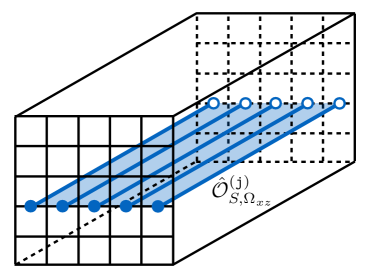
(b)

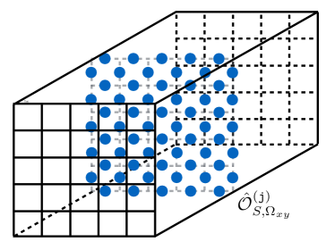
Figure 9: (Color online) Pictorial representations of the star-type membrane operators defined in Eqs. (46). In (a), the membrane is parallel to the $x$-$z$ plane (there is also a similarly-defined membrane parallel to the $y$-$z$ plane). In (b), the membrane is parallel to the $x$-$y$ plane. Plaquette-type membrane operators are represented similarly.

Second, for any $\texttt{j}=1,\cdots,M$ and any $0\leq z<L$, we define the non-local membrane operators

$$\hat{\mathcal{O}}^{(\texttt{j})}_{S,\Omega^{\,}_{xy}}(z)\,\raisebox{0.85pt}{.}\raisebox{2.85pt}{.}\!\!=\,\prod_{s^{\,}_{C}\in\Omega^{\,}_{xy}}\hat{S}^{(\texttt{j}){\dagger}}_{s^{\,}_{C}}(z),$$ (46a)

$$\hat{\mathcal{O}}^{(\texttt{j})}_{S,\Omega^{\,}_{xz}}\,\raisebox{0.85pt}{.}\raisebox{2.85pt}{.}\!\!=\,\prod_{s^{\,}_{C}\in\Gamma^{\,}_{x}}\hat{S}^{(\texttt{j}){\dagger}}_{s^{\,}_{C}}(0,L),$$ (46b)

$$\hat{\mathcal{O}}^{(\texttt{j})}_{S,\Omega^{\,}_{yz}}\,\raisebox{0.85pt}{.}\raisebox{2.85pt}{.}\!\!=\,\prod_{s^{\,}_{C}\in\Gamma^{\,}_{y}}\hat{S}^{(\texttt{j}){\dagger}}_{s^{\,}_{C}}(0,L),$$ (46c)

and

$$\hat{\mathcal{O}}^{(\texttt{j})}_{P,\Omega^{\,}_{\hat{x}\hat{y}}}(z)\,\raisebox{0.85pt}{.}\raisebox{2.85pt}{.}\!\!=\,\prod_{p^{\,}_{C}\in\Omega^{\,}_{\hat{x}\hat{y}}}\hat{P}^{(\texttt{j}){\dagger}}_{p^{\,}_{C}}(z),$$ (46d)

$$\hat{\mathcal{O}}^{(\texttt{j})}_{P,\Omega^{\,}_{\hat{x}\hat{z}}}\,\raisebox{0.85pt}{.}\raisebox{2.85pt}{.}\!\!=\,\prod_{p^{\,}_{C}\in\Gamma^{\,}_{\hat{x}}}\hat{P}^{(\texttt{j}){\dagger}}_{p^{\,}_{C}}(0,L),$$ (46e)

$$\hat{\mathcal{O}}^{(\texttt{j})}_{P,\Omega^{\,}_{\hat{y}\hat{z}}}\,\raisebox{0.85pt}{.}\raisebox{2.85pt}{.}\!\!=\,\prod_{p^{\,}_{C}\in\Gamma^{\,}_{\hat{y}}}\hat{P}^{(\texttt{j}){\dagger}}_{p^{\,}_{C}}(0,L).$$ (46f)

Here, $\Omega^{\,}_{xy}$ is a membrane covering all links of the square lattice in the $x$-$y$ plane at a constant $z$, while $\Omega^{\,}_{\hat{x}\hat{y}}$ is a membrane covering all links of the dual lattice in the $\hat{x}$-$\hat{y}$ plane at a constant $z$. The membranes $\Omega^{\,}_{xz}$ ($\Omega^{\,}_{\hat{x}\hat{z}}$) and $\Omega^{\,}_{yz}$ ($\Omega^{\,}_{\hat{y}\hat{z}}$) contain the non-contractible closed paths $\Gamma^{\,}_{x}$ ($\Gamma^{\,}_{\hat{x}}$) and $\Gamma^{\,}_{y}$ ($\Gamma^{\,}_{\hat{y}}$). Similarly to the string operators, these membrane operators can be interpreted as describing processes in which a linelike defect and its anti-defect are created as a pair, before one of the defects propagates along a non-contractible loop on the torus and annihilates with its partner. For pictorial representations of these membrane operators, see Fig. 9.

Neither the string operators (45) nor the membrane operators (46) create excitations, as understood in Sec. II.3.3, as the strings and membranes on which these operators act are always closed by virtue of the periodic boundary conditions we have imposed. Consequently, the string operators (45) and the membrane operators (46) commute with the Hamiltonian $\tilde{\hat{H}}^{\,}_{\mathrm{int}}\equiv-\tilde{\hat{L}}^{\,}_{\{\tilde{\mathcal{T}}\}}$ defined in Eq. (20).

For any $0\leq z<L$, the set of $12\,M$ string operators (45) and membrane operators (46) can be divided into two sets of $6\,M$, with the equivalent algebras

$$\hat{\mathcal{O}}^{(\texttt{j})}_{S,\Gamma^{\,}_{z}}\,\hat{\mathcal{O}}^{(\texttt{j}^{\prime})}_{P,\Omega^{\,}_{\hat{x}\hat{y}}}=\hat{\mathcal{O}}^{(\texttt{j}^{\prime})}_{P,\Omega^{\,}_{\hat{x}\hat{y}}}\,\hat{\mathcal{O}}^{(\texttt{j})}_{S,\Gamma^{\,}_{z}}\ e^{-\mathrm{i}\,2\pi\,\tilde{v}^{(\texttt{j})\mathsf{T}}\tilde{K}^{-1}\tilde{w}^{(\texttt{j}^{\prime})}},$$ (47a)

$$\hat{\mathcal{O}}^{(\texttt{j})}_{S,\Gamma^{\,}_{y}}\,\hat{\mathcal{O}}^{(\texttt{j}^{\prime})}_{P,\Omega^{\,}_{\hat{z}\hat{x}}}=\hat{\mathcal{O}}^{(\texttt{j}^{\prime})}_{P,\Omega^{\,}_{\hat{z}\hat{x}}}\,\hat{\mathcal{O}}^{(\texttt{j})}_{S,\Gamma^{\,}_{y}}\,e^{+\mathrm{i}\,2\pi\,\tilde{v}^{(\texttt{j})\mathsf{T}}\tilde{K}^{-1}\tilde{w}^{(\texttt{j}^{\prime})}},$$ (47b)

$$\hat{\mathcal{O}}^{(\texttt{j})}_{S,\Gamma^{\,}_{x}}\,\hat{\mathcal{O}}^{(\texttt{j}^{\prime})}_{P,\Omega^{\,}_{\hat{y}\hat{z}}}=\hat{\mathcal{O}}^{(\texttt{j}^{\prime})}_{P,\Omega^{\,}_{\hat{y}\hat{z}}}\,\hat{\mathcal{O}}^{(\texttt{j})}_{S,\Gamma^{\,}_{x}}\ e^{+\mathrm{i}\,2\pi\,\tilde{v}^{(\texttt{j})\mathsf{T}}\tilde{K}^{-1}\tilde{w}^{(\texttt{j}^{\prime})}},$$ (47c)

and

$$\hat{\mathcal{O}}^{(\texttt{j})}_{S,\Omega^{\,}_{xy}}\,\hat{\mathcal{O}}^{(\texttt{j}^{\prime})}_{P,\Gamma^{\,}_{\hat{z}}}=\hat{\mathcal{O}}^{(\texttt{j}^{\prime})}_{P,\Gamma^{\,}_{\hat{z}}}\,\hat{\mathcal{O}}^{(\texttt{j})}_{S,\Omega^{\,}_{xy}}\,e^{+\mathrm{i}\,2\pi\,\tilde{v}^{(\texttt{j})\mathsf{T}}\tilde{K}^{-1}\tilde{w}^{(\texttt{j}^{\prime})}},$$ (48a)

$$\hat{\mathcal{O}}^{(\texttt{j})}_{S,\Omega^{\,}_{zx}}\,\hat{\mathcal{O}}^{(\texttt{j}^{\prime})}_{P,\Gamma^{\,}_{\hat{y}}}=\hat{\mathcal{O}}^{(\texttt{j}^{\prime})}_{P,\Gamma^{\,}_{\hat{y}}}\,\hat{\mathcal{O}}^{(\texttt{j})}_{S,\Omega^{\,}_{zx}}\,e^{-\mathrm{i}\,2\pi\,\tilde{v}^{(\texttt{j})\mathsf{T}}\tilde{K}^{-1}\tilde{w}^{(\texttt{j}^{\prime})}},$$ (48b)

$$\hat{\mathcal{O}}^{(\texttt{j})}_{S,\Omega^{\,}_{yz}}\,\hat{\mathcal{O}}^{(\texttt{j}^{\prime})}_{P,\Gamma^{\,}_{\hat{x}}}=\hat{\mathcal{O}}^{(\texttt{j}^{\prime})}_{P,\Gamma^{\,}_{\hat{x}}}\,\hat{\mathcal{O}}^{(\texttt{j})}_{S,\Omega^{\,}_{yz}}\,e^{-\mathrm{i}\,2\pi\,\tilde{v}^{(\texttt{j})\mathsf{T}}\tilde{K}^{-1}\tilde{w}^{(\texttt{j}^{\prime})}},$$ (48c)

respectively. Note that all string and membrane operators associated with stars commute with one another, as do all string and membrane operators associated with plaquettes. Note also that there are, in principle, four equivalent copies of Eqs. (47a) and (48a), one for each choice of cardinal direction $C$ or $C^{\prime}$ in Eqs. (45c) and (45f), respectively. However, because we have chosen the vectors $\tilde{v}^{(\texttt{j})}$ and $\tilde{w}^{(\texttt{j}^{\prime})}$ in an isotropic way [i.e., by imposing the criterion (16)], these four copies of Eqs. (47a) and (48a) are redundant. We will henceforth work with fixed cardinalities $C$ and $C^{\prime}$ in Eqs. (45c) and (45f), respectively.

We are after the minimal topological ground-state degeneracy that is consistent with Eqs. (47) and (48). There are redundancies among the $12\,M$ operators defined in Eqs. (45) and (46) that reduce the total number of independent relations in Eqs. (47) and (48) to $3\,M$. For example, observe that

$$\hat{\mathcal{O}}^{(\texttt{j})}_{S,\Gamma^{\,}_{x}}\,\hat{\mathcal{O}}^{(\texttt{j}^{\prime})}_{P,\Gamma^{\,}_{\hat{z}}}=\hat{\mathcal{O}}^{(\texttt{j}^{\prime})}_{P,\Gamma^{\,}_{\hat{z}}}\,\hat{\mathcal{O}}^{(\texttt{j})}_{S,\Gamma^{\,}_{x}}\,e^{+\mathrm{i}\,2\pi\,\tilde{v}^{(\texttt{j})\mathsf{T}}\tilde{K}^{-1}\tilde{w}^{(\texttt{j}^{\prime})}}.$$ (49a)

It is consistent with Eqs. (47c) and (48a), to make either the identification $$\hat{\mathcal{O}}^{(\texttt{j})}_{S,\Gamma^{\,}_{x}}\equiv\hat{\mathcal{O}}^{(\texttt{j})}_{S,\Omega^{\,}_{xy}} \hat{\mathcal{O}}^{(\texttt{j}^{\prime})}_{P,\Gamma^{\,}_{\hat{z}}}\equiv\hat{\mathcal{O}}^{(\texttt{j}^{\prime})}_{P,\Omega^{\,}_{\hat{y}{\hat{z}}}} \texttt{j},\texttt{j}^{\prime}=1,\dots,M$$ or the identification for all when acting on the ground-state subspace. This indicates that one can remove either Eq. (47c) or Eq. (48a) from the algebra without changing the number of independent degrees of freedom. For concreteness, suppose we do away with Eq. (48a). Then, similarly, using the relations

$$\hat{\mathcal{O}}^{(\texttt{j})}_{S,\Gamma^{\,}_{z}}\,\hat{\mathcal{O}}^{(\texttt{j}^{\prime})}_{P,\Gamma^{\,}_{\hat{x}}}=\hat{\mathcal{O}}^{(\texttt{j}^{\prime})}_{P,\Gamma^{\,}_{\hat{x}}}\,\hat{\mathcal{O}}^{(\texttt{j})}_{S,\Gamma^{\,}_{z}}\,e^{-\mathrm{i}\,2\pi\,\tilde{v}^{(\texttt{j})\mathsf{T}}\tilde{K}^{-1}\tilde{w}^{(\texttt{j}^{\prime})}},$$ (49b)

$$\hat{\mathcal{O}}^{(\texttt{j})}_{S,\Gamma^{\,}_{z}}\,\hat{\mathcal{O}}^{(\texttt{j}^{\prime})}_{P,\Gamma^{\,}_{\hat{y}}}=\hat{\mathcal{O}}^{(\texttt{j}^{\prime})}_{P,\Gamma^{\,}_{\hat{y}}}\,\hat{\mathcal{O}}^{(\texttt{j})}_{S,\Gamma^{\,}_{z}}\,e^{-\mathrm{i}\,2\pi\,\tilde{v}^{(\texttt{j})\mathsf{T}}\tilde{K}^{-1}\tilde{w}^{(\texttt{j}^{\prime})}},$$ (49c)

we can remove Eqs. (48b) and (48c) from the algebra. With the redundant operators removed, we are left with a set of $6\,M$ nonlocal operators obeying the algebra of Eqs. (47).

The ground-state degeneracy on the three-torus

$$\mathbb{T}^{3}\equiv S^{1}\times S^{1}\times S^{1}$$ (50)

in the strong coupling limit where the kinetic contribution to the Hamiltonian $\tilde{\hat{H}}$ defined in Eq. (20) is much smaller than the contribution from $\tilde{\hat{H}}^{\,}_{\mathrm{int}}\equiv-\tilde{\hat{L}}^{\,}_{\{\tilde{\mathcal{T}}\}}$ can be deduced from the algebra (47) as follows. Close to the limit $\tilde{\hat{H}}=\tilde{\hat{H}}^{\,}_{\mathrm{int}}$, the ground-state manifold must transform as a representation of the algebra (47). If so, the representation of the algebra (47) with the smallest dimension determines the minimal topological ground-state degeneracy. Equations (47) consist of three independent copies of the generalized “magnetic algebra,” which is ubiquitous in studies of the ground-state degeneracy of abelian topological states of matter Wen (1991); Wen and Zee (1992); Wesolowski et al. (1994). The minimum-dimensional representation of any one of the three algebras in Eqs. (47) has dimension $|\det\varkappa|$, where

$$\varkappa^{-1}_{\texttt{j}\texttt{j}^{\prime}}\,\raisebox{0.85pt}{.}\raisebox{2.85pt}{.}\!\!=\,\tilde{v}^{(\texttt{j})\mathsf{T}}\,\tilde{K}^{-1}\,\tilde{w}^{(\texttt{j}^{\prime})}=\frac{\theta^{\,}_{\texttt{j}\texttt{j}^{\prime}}}{2\pi}$$ (51)

is an $M\times M$-dimensional symmetric matrix foo . We conclude that the class of coupled wires considered in this work has a ground-state degeneracy $D^{\,}_{\mathbb{T}^{3}}$ on the three-torus given by

$$D^{\,}_{\mathbb{T}^{3}}=|\det\varkappa|^{3}.$$ (52)

Combining Eq. (52) with the definition of the matrix $\varkappa$ provided in Eq. (51), one can verify the claim made earlier in this section, namely that $D^{\,}_{\mathbb{T}^{3}}=1$ if $|\det\tilde{K}=1|$. To see this, recall that the inverse of the matrix $\tilde{K}$ is given by

$$\tilde{K}^{-1}=\frac{1}{\det\,\tilde{K}}\,C^{\,}_{\tilde{K}},$$ (53)

where $C^{\,}_{\tilde{K}}$ is the cofactor matrix associated with $\tilde{K}$. Since $\tilde{K}$ is an integer-valued matrix, it follows that $C^{\,}_{\tilde{K}}$ is also integer valued, and that $\det\,\tilde{K}$ is an integer. Combining these facts with our assumptions that $\tilde{v}^{(\texttt{j})}$ and $\tilde{w}^{(\texttt{j})}$ are integer-valued and that $\det\,\tilde{K}=\pm 1$, one concludes that $\varkappa^{-1}_{\texttt{j}\texttt{j}^{\prime}}$ is an integer for all j and $\texttt{j}^{\prime}=1,\ldots,M$. Consequently, each line of Eqs. (47) becomes a trivial commutation relation for all j and $\texttt{j}^{\prime}$, and we conclude that $D^{\,}_{\mathbbm{T}^{3}}=1$.

Nontrivial states of matter for which $\det D^{\,}_{\mathbb{T}^{3}}=1$ are examples of short-range entangled (SRE) or symmetry-protected topological (SPT) states of matter Pollmann et al. (2010); Chen et al. (2013). Although such states of matter do not yield quasiparticle excitations with fractionalized charges or statistics, and are therefore not of primary interest to us here, they are nevertheless readily treated within the formalism developed in this paper.

II.3.7 Topological field theory

We close the discussion of the general class of three-dimensional wire constructions considered in this work by commenting on the topological field theory characterizing the low-energy behavior of these theories. In the study of the braiding statistics of quasiparticle excitations undertaken in Sec. II.3.5, we found that these wire constructions host both pointlike and stringlike excitations of $M$ types, labeled by $\texttt{j}=1,\ldots,M$. We also observed that winding a pointlike defect of type j around a stringlike defect of type $\texttt{j}^{\prime}$ yields a statistical phase $\theta^{\,}_{\texttt{j}\texttt{j}^{\prime}}$, and that all other statistical phases were trivial.

We wish to capture this statistical “interaction” between quasiparticles with a topological field theory, in a manner similar to the way in which Chern-Simons (CS) theories in (2+1) dimensions can be used to encode the statistics of pointlike quasiparticles. Studies of topologically-ordered superconductors Hansson et al. (2004) and (3+1)-dimensional topological insulators Cho and Moore (2011); Chan et al. (2013) have shown that the statistics of theories where pointlike excitations acquire a nontrivial phase when encircling vortex lines can be encoded in so-called BF theories. For example, in a (3+1)-dimensional topolgical insulator, the statistical phase of $\pi$ that a quasiparticle acquires when it circles a vortex line is encoded in the BF Lagrangian density Hansson et al. (2004); Cho and Moore (2011); Tiwari et al. (2014)

$$\mathcal{L}^{\,}_{\mathrm{BF}} \,\raisebox{0.85pt}{.}\raisebox{2.85pt}{.}\!\!=\,\frac{1}{2\pi}\,\epsilon^{\mu\nu\rho\lambda}\,a^{\,}_{\mu}\,\partial^{\,}_{\nu}\,b^{\,}_{\rho\lambda},$$ (54)

where $\mu=t,x,y,z$ runs over all spacetime indices, $\epsilon^{\mu\nu\rho\lambda}$ is the fully antisymmetric Levi-Civita symbol, and summation over repeated Greek indices is implied. Here, the one-form $a^{\,}_{\mu}$ is an emergent gauge field that couples to the quasiparticle current density, and $b^{\,}_{\mu\nu}$ is an antisymmetric two-form that couples to the vortex-line density. The natural generalization of this BF Lagrangian to our setting is obtained by introducing $M$ species of one-forms $a^{(\texttt{j})}_{\mu}$ and $M$ species of two-forms $b^{(\texttt{j})}_{\mu\nu}$, one for each type of pointlike and stringlike excitation, respectively. This results in the multicomponent BF Lagrangian density

$$\mathcal{L}^{\,}_{\mathrm{BF}}\,\raisebox{0.85pt}{.}\raisebox{2.85pt}{.}\!\!=\,\frac{\varkappa^{\,}_{\texttt{j}\texttt{j}^{\prime}}}{4\pi}\,\epsilon^{\mu\nu\rho\lambda}\,a^{(\texttt{j})}_{\mu}\,\partial^{\,}_{\nu}\,b^{(\texttt{j}^{\prime})}_{\rho\lambda},$$ (55)

where the $M\times M$ matrix $\varkappa$ is defined in Eq. (51) and summation over repeated Greek and teletype indices is implied. This discussion indicates that the class of coupled wires considered so far falls into the same equivalence class of topological states of matter as the (3+1)-dimensional fractional topological insulators Swingle et al. (2011); Maciejko et al. (2010, 2014); Tiwari et al. (2014); Sagi and Oreg (2015). This is consistent with the example of $\mathbb{Z}^{\,}_{m}$ topological order in three spatial dimensions that we discuss in the next section.

Before moving on, we address the question of how this discussion would have been different if we had instead considered the more general case $\tilde{v}^{(\texttt{j})}_{1}\neq\tilde{v}^{(\texttt{j})}_{2}$ and $\tilde{w}^{(\texttt{j})}_{1}\neq\tilde{w}^{(\texttt{j})}_{2}$ [recall Eqs. (15) and (17)]. As we observed after Eq. (40), this more general case requires us to impose the consistency condition (41) in order for the statistics of pointlike and linelike excitations to be well-defined. However, because, in this case, there is a well-defined statistical angle $\theta^{\,}_{\texttt{j}\texttt{j}^{\prime}}$, one may define the matrix $\varkappa^{-1}_{\texttt{j}\texttt{j}^{\prime}}$ in terms of $\theta^{\,}_{\texttt{j}\texttt{j}^{\prime}}$ by making use of the relation (51), leading again to the multicomponent BF theory defined in Eq. (55). This observation can be taken as a justification a posteriori for considering from the outset, as we did, the simpler class of models in which $\tilde{v}^{(\texttt{j})}_{1}=\tilde{v}^{(\texttt{j})}_{2}=\tilde{v}^{(\texttt{j})}$ and $\tilde{w}^{(\texttt{j})}_{1}=\tilde{w}^{(\texttt{j})}_{2}=\tilde{w}^{(\texttt{j})}$.

II.4 Example: $\mathbb{Z}^{\,}_{m}$ topological order in three-dimensional space from coupled wires

Having developed a toolbox for the construction of a class of two-dimensional arrays of coupled quantum wires, we now turn to an illustration of this framework in action. In this section, we show how to realize the simplest type of three-dimensional topological order, namely $\mathbb{Z}^{\,}_{m}$ topological order, within the wire formalism developed in the previous sections. This class of examples includes the three-dimensional toric code, which is an example of $\mathbb{Z}^{\,}_{2}$ topological order.

II.4.1 Definitions and interwire couplings

Our starting point is a set of $2N$ decoupled two-component bosonic quantum wires placed on the links of a square lattice. (We will also discuss momentarily how one can arrive at a class of $\mathbbm{Z}^{\,}_{2m}$-topologically-ordered states starting from fermions, although it turns out to be simpler to focus on the bosonic case.) We take the decoupled quantum wires to be described by the Lagrangian (1) with

$$\mathcal{K}\,\raisebox{0.85pt}{.}\raisebox{2.85pt}{.}\!\!=\,\mathbbm{1}^{\,}_{2N}\otimes K^{\,}_{\mathrm{b}},$$ (56a)

where $$K^{\,}_{\mathrm{b}} M=1 K^{\,}_{\mathrm{b}} 2\times 2 K$$ was defined in Eq. (3b), and we take so that is a matrix. With the -matrix defined in this way, the canonical equal-time commutation relation for the theory of decoupled wires is given by

$$\begin{split}\left[\partial^{\,}_{z}\hat{\phi}^{\,}_{j,1}(z),\hat{\phi}^{\,}_{j^{\prime},2}(z^{\prime})\right]&=\mathrm{i}\,2\pi\,\delta^{\,}_{jj^{\prime}}\,\delta(z-z^{\prime})\\ &=\left[\partial^{\,}_{z}\hat{\phi}^{\,}_{j,2}(z),\hat{\phi}^{\,}_{j^{\prime},1}(z^{\prime})\right].\end{split}$$ (56b)

The charge vector that fixes the coupling of the two bosonic fields $$\hat{\phi}^{\,}_{j,1} \hat{\phi}^{\,}_{j,2}$$ and to external gauge potentials is given by

$$Q^{\,}_{\mathrm{b}}\,\raisebox{0.85pt}{.}\raisebox{2.85pt}{.}\!\!=\,2\begin{pmatrix}1&0\end{pmatrix}^{\mathsf{T}},$$ (56c)

so that $\hat{\phi}^{\,}_{j,1}$ can be interpreted as the “charge” mode and $\hat{\phi}^{\,}_{j,2}$ can be interpreted as the “spin” mode.

It is convenient to write down the interwire couplings for this model in the new basis defined by the transformation (18) with

$$W\,\raisebox{0.85pt}{.}\raisebox{2.85pt}{.}\!\!=\,\mathrm{diag}(1,m),$$ (57a)

so that the transformed $$K$$-matrix and charge-vector are given by

$$\tilde{K}^{\,}_{m}\,\raisebox{0.85pt}{.}\raisebox{2.85pt}{.}\!\!=\,\begin{pmatrix}0&m\\ m&0\end{pmatrix},$$ (57b)

$$\tilde{Q}\,\raisebox{0.85pt}{.}\raisebox{2.85pt}{.}\!\!=\,Q^{\,}_{\mathrm{b}}.$$ (57c)

In this example, we will impose time-reversal symmetry (TRS), which constrains the allowed interwire couplings. TRS acts on the bosonic fields as

$$\tilde{\hat{\phi}}_{j,\alpha}(t,z)\mapsto(-1)^{\alpha-1}\,\tilde{\hat{\phi}}_{j,\alpha}(-t,z)$$ (58)

for all $j=1,\dots 2N$ and $\alpha=1,2$. Note that this is not the only possible choice for the action of TRS (see, e.g., Ref. Neupert et al. (2011)), but that this representation of TRS squares to unity, as expected for bosons.

Before proceeding to write down the interwire couplings, we first point out that a theory similar to the one defined by the universal data (57) can also be reached starting from wires supporting spinless fermions defined by the data

$$K^{\,}_{\mathrm{f}}\,\raisebox{0.85pt}{.}\raisebox{2.85pt}{.}\!\!=\,\begin{pmatrix}+1&0\\ 0&-1\end{pmatrix},$$ (59a)

$$Q^{\,}_{\mathrm{f}}\,\raisebox{0.85pt}{.}\raisebox{2.85pt}{.}\!\!=\,\begin{pmatrix}1&1\end{pmatrix}^{\mathsf{T}},$$ (59b)

using the transformation

$$W^{\prime}\,\raisebox{0.85pt}{.}\raisebox{2.85pt}{.}\!\!=\,\begin{pmatrix}-1&-m\\ -1&+m\end{pmatrix}.$$ (60)

In this alternative interpretation of Eqs. (57), we view the original bosons as being composite objects consisting of paired fermions, since the transformed $K$-matrix and charge vector read

$$\tilde{K}^{\prime}_{m}\,\raisebox{0.85pt}{.}\raisebox{2.85pt}{.}\!\!=\,W^{\prime\mathsf{T}}\,K^{\,}_{\mathrm{f}}\,W^{\prime}=2\,\tilde{K}^{\,}_{m},$$ (61a)

$$\tilde{Q}^{\prime}_{m}\,\raisebox{0.85pt}{.}\raisebox{2.85pt}{.}\!\!=\,W^{\prime\mathsf{T}}\,Q^{\,}_{\mathrm{f}}=-Q^{\,}_{\mathrm{b}}.$$ (61b)

The additional multiplicative factors of $2$ on the right-hand sides of the above equations can be seen as evidence of this pairing. Furthermore, the action of TRS on the bosonic fields after performing the transformation (60) is still given by (58), indicating that the theory defined by the data (61) and the theory defined by the data (57) transform in the same way under TRS.

Hence, although we choose to focus here on the bosonic case, with universal data given by Eqs. (57), all results that follow could be interpreted as arising from paired fermions, so long as $m$ is taken to be even.

(a)

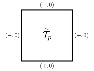
(b)

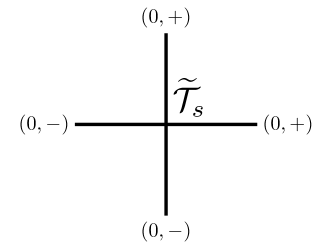
Figure 10: Pictorial representations of the tunneling vectors (a) $\tilde{\mathcal{T}}^{\,}_{s}$ and (b) $\tilde{\mathcal{T}}^{\,}_{p}$ built using the vectors $\tilde{v}$ and $\tilde{w}$ defined in Eqs. (62). The signs $\pm$ indicate whether a $\pm 1$ appears in the tunneling vector associated with that link.

We couple the $2N$ quantum wires with a Lagrangian $\tilde{\hat{L}}^{\,}_{\{\tilde{\mathcal{T}}\}}$, defined as in Eq. (7), for tunneling vectors $\tilde{\mathcal{T}}$ defined as in Eqs. (13) with (see Fig. 10)

$$\tilde{v}^{\,}_{1}\equiv\tilde{v}^{\,}_{2}\equiv\tilde{v}\,\raisebox{0.85pt}{.}\raisebox{2.85pt}{.}\!\!=\,\begin{pmatrix}0&+1\end{pmatrix}^{\mathsf{T}},$$ (62a)

$$\tilde{w}^{\,}_{1}\equiv\tilde{w}^{\,}_{2}\equiv\tilde{w}\,\raisebox{0.85pt}{.}\raisebox{2.85pt}{.}\!\!=\,\begin{pmatrix}-1&0\end{pmatrix}^{\mathsf{T}}.$$ (62b)

It is readily verified that these tunneling vectors satisfy the criteria (17), which ensure that the interaction terms in $\tilde{\hat{L}}^{\,}_{\{\tilde{\mathcal{T}}\}}$ are sufficient to gap out the array of quantum wires when periodic boundary conditions are imposed. Furthermore, the cosine terms associated with the tunneling vectors (62) are even under TRS, as desired.

II.4.2 Excitations

Excitations of the array of coupled wires can be constructed using the procedure outlined in Sec. II.3.3.

First, we define the local vertex operators

$$\hat{S}^{{\dagger}}_{s^{\,}_{C}}(z)\,\raisebox{0.85pt}{.}\raisebox{2.85pt}{.}\!\!=\,\exp\left(-\mathrm{i}\,\tilde{\hat{\phi}}^{\,}_{s^{\,}_{C},2}(z)\right)$$ (63a)

and

$$\hat{P}^{{\dagger}}_{p^{\,}_{C}}(z)\,\raisebox{0.85pt}{.}\raisebox{2.85pt}{.}\!\!=\,\exp\left(+\mathrm{i}\,\tilde{\hat{\phi}}^{\,}_{p^{\,}_{C},1}(z)\right).$$ (63b)

These vertex operators are eigenstates of the charge operator $\tilde{\hat{Q}}^{\,}_{j,\alpha}$ defined in Eq. (26) with the $\tilde{K}$ matrix (61a) and the charge vector (61b), respectively. Indeed, following the derivation of Eq. (27), we find the equal-time commutators

$$\left[\tilde{\hat{Q}}^{\,}_{j,\alpha},\hat{S}^{{\dagger}}_{s^{\,}_{C}}(z)\right]=+\frac{2}{m}\,\delta^{\,}_{j,s^{\,}_{C}}\,\delta^{\,}_{\alpha,1}\,\hat{S}^{{\dagger}}_{s^{\,}_{C}}(z),$$ (64a)

$$\left[\tilde{\hat{Q}}^{\,}_{j,\alpha},\hat{P}^{{\dagger}}_{p^{\,}_{C}}(z)\right]=0.$$ (64b)

The meaning of Eq. (64a) is that the vertex operator $\hat{S}^{{\dagger}}_{s^{\,}_{C}}(z)$ creates along the wire $j$ piercing the midpoint of the bond $s^{\,}_{C}$ ($C=N,W,S,E$) belonging to the star $s$ an excitation with charge $2/m$ for the flavor $\alpha=1$. The meaning of Eq. (64b) is that $\hat{P}^{{\dagger}}_{s^{\,}_{C}}(z)$ creates a charge-neutral excitation.

A second attribute of these quasi-particle operators is that they create fractional kinks in the charge-neutral operators

$$\begin{split}\hat{T}^{\,}_{s}(z)\,\raisebox{0.85pt}{.}\raisebox{2.85pt}{.}\!\!=\,&\,\frac{1}{m}\,\tilde{\mathcal{T}}^{\mathsf{T}}_{s}\,\tilde{\mathcal{K}}^{\,}_{m}\tilde{\hat{\Phi}}(z)\\ =&\,\tilde{\hat{\phi}}^{\,}_{s^{\,}_{E},1}(z)-\tilde{\hat{\phi}}^{\,}_{s^{\,}_{W},1}(z)+\tilde{\hat{\phi}}^{\,}_{s^{\,}_{N},1}(z)-\tilde{\hat{\phi}}^{\,}_{s^{\,}_{S},1}(z)\end{split}$$ (65a)

and

$$\begin{split}\hat{T}^{\,}_{p}(z)\,\raisebox{0.85pt}{.}\raisebox{2.85pt}{.}\!\!=\,&\,\frac{1}{m}\tilde{\mathcal{T}}^{\mathsf{T}}_{p}\,\tilde{\mathcal{K}}^{\,}_{m}\tilde{\hat{\Phi}}(z)\\ =&\,\tilde{\hat{\phi}}^{\,}_{p^{\,}_{E},2}(z)-\tilde{\hat{\phi}}^{\,}_{p^{\,}_{W},2}(z)+\tilde{\hat{\phi}}^{\,}_{p^{\,}_{S},2}(z)-\tilde{\hat{\phi}}^{\,}_{p^{\,}_{N},2}(z),\end{split}$$ (65b)

respectively. Indeed, application of Eqs. (32) and (35) in combination with Eq. (62) delivers

$$\hat{S}^{\,}_{s^{\,}_{C}}(z^{\prime})\,\hat{T}^{\,}_{s^{\prime}}(z)\,\hat{S}^{{\dagger}}_{s^{\,}_{C}}(z^{\prime})=\hat{T}^{\,}_{s^{\prime}}(z)+\sigma^{\,}_{s,s^{\prime};C}\,\frac{2\pi}{m}\,\Theta(z-z^{\prime}),$$ (66a)

where we have introduced the function $$\sigma^{\,}_{s,s^{\prime};C} s=s^{\prime} s s^{\prime} s^{\,}_{C}$$ that returns the signs multiplying the Heaviside step functions on the right-hand side of Eq. (32) if , the signs multiplying the Heaviside step functions on the right-hand side of Eq. (35) if and share , and zero otherwise. Similarly, application of Eqs. (33) and (36), in combination with Eq. (62) delivers

$$\hat{P}^{\,}_{p^{\,}_{C}}(z^{\prime})\,\hat{T}^{\,}_{p^{\prime}}(z)\,\hat{P}^{{\dagger}}_{p^{\,}_{C}}(z^{\prime})=\hat{T}^{\,}_{p^{\prime}}(z)+\sigma^{\,}_{p,p^{\prime};C}\,\frac{2\pi}{m}\,\Theta(z-z^{\prime}),$$ (66b)

where we have introduced the function $\sigma^{\,}_{p,p^{\prime};C}$ that returns the signs multiplying the Heaviside step functions on the right-hand side of Eq. (33) if $p=p^{\prime}$, the signs multiplying the Heaviside step functions on the right-hand side of Eq. (36) if $p$ and $p^{\prime}$ share $p^{\,}_{C}$, and zero otherwise.

If we define the soliton density operator for any star $s$ in the square lattice by

$$\hat{\rho}^{\mathrm{sol}}_{s}(z)\,\raisebox{0.85pt}{.}\raisebox{2.85pt}{.}\!\!=\,\frac{1}{2\pi}\left(\partial^{\,}_{z}\hat{T}^{\,}_{s}\right)(z)$$ (67a)

and do the same with

$$\hat{\rho}^{\mathrm{sol}}_{p}(z)\,\raisebox{0.85pt}{.}\raisebox{2.85pt}{.}\!\!=\,\frac{1}{2\pi}\left(\partial^{\,}_{z}\hat{T}^{\,}_{p}\right)(z)$$ (67b)

for any plaquette $p$ in the square lattice, we can then make the substitutions $\hat{T}^{\,}_{s^{\prime}}\to\hat{\rho}^{\mathrm{sol}}_{s^{\prime}}$, $\hat{T}^{\,}_{p^{\prime}}\to\hat{\rho}^{\mathrm{sol}}_{p^{\prime}}$, and $2\pi\,\Theta(z-z^{\prime})\to\delta(z-z^{\prime})$ in Eqs. (66a) and (66b), respectively. The resulting pair of equations is interpreted as the fact that any one of the pair of operators $\hat{S}^{{\dagger}}_{s^{\,}_{C}}(z)$ and $\hat{P}^{{\dagger}}_{p^{\,}_{C}}(z)$ creates a dipole with a soliton charge of magnitude $1/m$ straddling the link $s^{\,}_{C}$ or $p^{\,}_{C}$ with the cardinality $C=N,W,S,E$ belonging to the star $s$ and plaquette $p$, respectively. Upon multiplying $\hat{\rho}^{\mathrm{sol}}_{s}$ and $\hat{\rho}^{\mathrm{sol}}_{p}$ by the electric charges $\tilde{Q}^{\,}_{1}=2$ and $\tilde{Q}^{\,}_{2}=0$, respectively, we conclude that $\hat{S}^{{\dagger}}_{s^{\,}_{C}}(z)$ creates an electric dipole with a charge of magnitude $2/m$ straddling the link$s^{\,}_{C}$ with the cardinality $C=N,W,S,E$ belonging to the star $s$. On the other hand, the operator $\hat{P}^{{\dagger}}_{p^{\,}_{C}}(z)$ creates an electrically neutral dipole. Hence, anticipating a connection to 3D toric code models that we will demonstrate shortly, we refer to the charged constituents of the electric dipole created by the operator $\hat{S}^{{\dagger}}_{s^{\,}_{C}}(z)$ as “electric” excitations, and to the constituents of the neutral dipole greated by the operator $\hat{P}^{{\dagger}}_{p^{\,}_{C}}(z)$ as “magnetic” excitations.

Second, the bilocal operators

$$\begin{split}\hat{S}^{{\dagger}}_{s^{\,}_{C}}(z^{\,}_{1},z^{\,}_{2})&\,\raisebox{0.85pt}{.}\raisebox{2.85pt}{.}\!\!=\,\hat{S}^{{\dagger}}_{s^{\,}_{C}}(z^{\,}_{2})\,\hat{S}^{\phantom{{\dagger}}}_{s^{\,}_{C}}(z^{\,}_{1})\\ &=\exp\bigg{(}-\mathrm{i}\,\int\limits^{z^{\,}_{2}}_{z^{\,}_{1}}\mathrm{d}z\ \partial^{\,}_{z}\tilde{\hat{\phi}}^{\,}_{s^{\,}_{C},2}(z)\bigg{)},\end{split}$$ (68a)

and

$$\begin{split}\hat{P}^{{\dagger}}_{p^{\,}_{C}}(z^{\,}_{1},z^{\,}_{2})&\,\raisebox{0.85pt}{.}\raisebox{2.85pt}{.}\!\!=\,\hat{P}^{{\dagger}}_{p^{\,}_{C}}(z^{\,}_{2})\,\hat{P}^{\phantom{{\dagger}}}_{p^{\,}_{C}}(z^{\,}_{1})\\ &=\exp\bigg{(}+\mathrm{i}\,\int\limits^{z^{\,}_{2}}_{z^{\,}_{1}}\mathrm{d}z\ \partial^{\,}_{z}\tilde{\hat{\phi}}^{\,}_{p^{\,}_{C},1}(z)\bigg{)},\end{split}$$ (68b)

can be used to create and propagate linelike defects that extend in the $z$-direction, as in Fig. 5(a) and (b). Linelike defects lying in the $x$-$y$ plane can be created and propagated by repeated application of the vertex operators in Eqs. (63), as in the example of Fig. 5(c) and (d).

The statistical angle $\theta$ obtained upon winding of the pointlike and linelike excitations created by these operators can be computed from Eq. (40), which gives

$$\theta=-2\pi/m.$$ (69)

The case $m=2$ produces the expected statistical phase of $\pi$ between “electric” quasiparticles and “magnetic” strings in the 3D toric code. We will see this resemblance borne out in the next section, where we compute the ground state degeneracy.

II.4.3 Ground state degeneracy on the three-torus

The nonlocal string and membrane operators used to obtain the ground state degeneracy on the three-torus $\mathbb{T}^{3}$ for this example can be assembled from the vertex operators defined in Eqs. (63) and the bilocal operators defined in Eqs. (68), as outlined in Sec. II.3.6. As discussed in Sec. II.3.6, it is sufficient to consider the algebra of star-type string operators and plaquette-type membrane operators to deduce the degeneracy. This is given by

$$\hat{\mathcal{O}}^{\,}_{S,\Gamma^{\,}_{z}}\,\hat{\mathcal{O}}^{\,}_{P,\Omega^{\,}_{\hat{x}\hat{y}}}=\hat{\mathcal{O}}^{\,}_{P,\Omega^{\,}_{\hat{x}\hat{y}}}\,\hat{\mathcal{O}}^{\,}_{S,\Gamma^{\,}_{z}}\ e^{+\mathrm{i}\,2\pi/m},$$ (70a)

$$\hat{\mathcal{O}}^{\,}_{S,\Gamma^{\,}_{y}}\,\hat{\mathcal{O}}^{\,}_{P,\Omega^{\,}_{\hat{z}\hat{x}}}=\hat{\mathcal{O}}^{\,}_{P,\Omega^{\,}_{\hat{z}\hat{x}}}\,\hat{\mathcal{O}}^{\,}_{S,\Gamma^{\,}_{y}}\,e^{-\mathrm{i}\,2\pi/m},$$ (70b)

$$\hat{\mathcal{O}}^{\,}_{S,\Gamma^{\,}_{x}}\,\hat{\mathcal{O}}^{\,}_{P,\Omega^{\,}_{\hat{y}\hat{z}}}=\hat{\mathcal{O}}^{\,}_{P,\Omega^{\,}_{\hat{y}\hat{z}}}\,\hat{\mathcal{O}}^{\,}_{S,\Gamma^{\,}_{x}}\ e^{-\mathrm{i}\,2\pi/m}.$$ (70c)

[See Eqs. (45) and (46) for definitions of these operators.] Each line of Eqs. (70) contributes an $m$-fold topological degeneracy, for a total degeneracy on the three-torus

$$D^{\,}_{\mathbb{T}^{3}}=m^{3}.$$ (71)

Note that for $m=2$, which corresponds to the case of $\mathbb{Z}^{\,}_{2}$ topological order, the ground-state degeneracy is 8-fold. This is the expected topological degeneracy of the three-dimensional toric code Castelnovo and Chamon (2008); Mazáč and Hamma (2012), which is an important sanity check.

II.4.4 Surface states

All properties that we have discussed so far pertain to the bulk of the array of coupled wires, as we have always imposed periodic boundary conditions in all spatial directions. However, the wire formalism provides means to address the surface states as well. We first illustrate this fact with the example of the $\mathbb{Z}^{\,}_{m}$ theories discussed in this section, before commenting on surface states in more generality.

Figure 11: (Color online) Example of an array of quantum wires with open boundary conditions in the $y$-direction and periodic boundary conditions along all other directions. The dashed links indicate the presence of periodic boundary conditions in the $x$-direction. The crosses represent quantum wires on the links of the square lattice that are inequivalent modulo the periodic boundary conditions. In this example, $N^{\,}_{x}=3$ and $N^{\,}_{y}=2$. Consequently, there are $2\,N^{\,}_{x}\,N^{\,}_{y}+N^{\,}_{x}=15$ wires in the array, and $2\,N^{\,}_{x}\,N^{\,}_{y}-N^{\,}_{x}=9$ wires are gapped by the allowed tunneling vectors. Consequently, there are $6$ wires in the array that remain gapless when these tunneling vectors are included (3 on the top face and 3 on the bottom face, represented by the purple crosses).

Let us begin by relaxing the constraint of periodic boundary conditions that we have imposed until now. We choose open boundary conditions in the $y$-direction, while leaving periodic boundary conditions in the $x$ and $z$-directions. In this case, the surface of the system has the same topology as the two-torus

$$\mathbb{T}^{2}\,\raisebox{0.85pt}{.}\raisebox{2.85pt}{.}\!\!=\,S^{1}\times S^{1}.$$ (72)

The latter can be viewed as a plane parallel to the $x$-$z$ plane whose adjacent sides have been identified. There are two types of surface terminations of the square lattice whose links host the constituent quantum wires in the array. These are “rough” boundaries, which consist of stars, and “smooth” boundaries, which consist of plaquettes. For the sake of specificity, we will focus on “smooth” boundaries, as in Fig. 11, for the time being. All statements that we make about “smooth” boundaries below have analogs for the case of rough boundaries. However, the differences between the two types of boundary are not always physically insignificant, as we will provide shortly an example of a difference between rough and smooth boundaries.

The effects of imposing these semi-open boundary conditions are twofold. First, they increase the number of gapless degrees of freedom in the array of coupled wires, as the wires along the terminating surfaces of the wire array are no longer identified with each other. Second, they decrease the number of tunneling vectors in the Haldane set $\mathbb{H}$, as any stars or plaquettes that were formerly completed by virtue of the periodicity of the array of wires are now nonlocal, and therefore cannot be included. This results in a number, which we will determine momentarily, of “extra” gapless modes on the terminating surfaces of the array of coupled wires.

We can determine the existence of gapless surface states for the coupled-wire theory defined in Sec. II.4.1 by the following counting argument. First, recall that, when periodic boundary conditions are imposed, the square lattice contains $2N$ quantum wires, placed on its links. Let us write $N\equiv N^{\,}_{x}\times N^{\,}_{y}$, where $N^{\,}_{x}$ counts either the number of stars or the number of plaquettes along the $x$-direction. The number $N^{\,}_{y}$ does the same along the $y$-direction. When periodic boundary conditions are relaxed along the $y$-direction, the wires along the bottom and top faces of the array of wires (see Fig. 11) are no longer identified with one another, which adds $N^{\,}_{x}$ wires to the array. The total number of wires in the array with the topology (72) is therefore

$$2\,N^{\,}_{x}\,N^{\,}_{y}+\,N^{\,}_{x},$$ (73a)

and the associated number of gapless degrees of freedom is

$$4\,N^{\,}_{x}\,N^{\,}_{y}+2\,N^{\,}_{x}.$$ (73b)

Next, we count the number of available tunneling vectors in the array of wires when the topology (72) is imposed. Before relaxing periodic boundary conditions, there are $2\,N^{\,}_{x}\,N^{\,}_{y}$ tunneling vectors in the Haldane set $\mathbb{H}$, which is sufficient to gap out all $4\,N^{\,}_{x}\,N^{\,}_{y}$ degrees of freedom when periodic boundary conditions are imposed. However, when periodic boundary conditions are relaxed in the $y$-direction, $N^{\,}_{x}$ tunneling vectors must be removed from the set $\mathbb{H}$. Consequently, the total number of degrees of freedom left once all allowed tunneling vectors are included is given by

$$4\,N^{\,}_{x}\,N^{\,}_{y}+2\,N^{\,}_{x}-(4\,N^{\,}_{x}\,N^{\,}_{y}-2\,N^{\,}_{x})=4\,N^{\,}_{x}.$$ (74)

Since the remaining degrees of freedom must live on the boundary, where we have deleted tunneling vectors from the set $\mathbb{H}$, we can split the remaining $4\,N^{\,}_{x}$ degrees of freedom evenly among the top and bottom edges of the array of wires. This simply leaves $N^{\,}_{x}$ gapless quantum wires on each exposed surface, i.e., $2\,N^{\,}_{x}$ gapless degrees of freedom on each of the top and bottom surfaces, respectively. (An example of this counting procedure is shown in Fig. 11.)

It is a nontrivial task to determine the exact surface Lagrangian governing the remaining $2\,N^{\,}_{x}$ gapless degrees of freedom on each terminating surface of the array of wires. For example, in the case of Fig. 11, it is tempting to deduce that the surface Lagrangian describes a theory of decoupled quantum wires built out of the fields $\tilde{\hat{\phi}}^{\,}_{i,1}$ that no longer enter any cosine terms due to the removal of the “three-legged” stars that lie on the terminating surfaces, and their conjugate fields $\tilde{\hat{\phi}}^{\,}_{i,2}$. However, the latter fields couple to the bulk of the array of quantum wires via cosine terms associated with the plaquettes that lie along the terminating surfaces. Consequently, the fields $\tilde{\hat{\phi}}^{\,}_{i,1}$ and $\tilde{\hat{\phi}}^{\,}_{i,2}$ do not provide the right basis for the gapless surface states.

However, despite the difficulty of determining a Lagrangian description of these gapless surface states, the determination of the stability of these surface states and the characterization of any proximal gapped phases are readily feasible with the tools already developed in this work.

The stability of the gapless surfaces can be addressed by seeking out a set of $2\,N^{\,}_{x}$ tunneling vectors, i.e., $N^{\,}_{x}$ tunneling vectors for each terminating surface, to complete the Haldane set $\mathbb{H}$. These surface tunneling vectors must be chosen to comply with all symmetries of the problem, in this case TRS and charge conservation, and must be compatible with the bulk tunneling vectors in the sense of the Haldane criterion (11). If any number less than $N^{\,}_{x}$ tunneling vectors for each terminating surface is found, then the gapless surface states are stable, since it is impossible to localize all gapless degrees of freedom in the array of quantum wires with the topology (72), while simultaneously preserving all symmetries. If, instead, the necessary number of compatible tunneling vectors is found, then the gapless surface states are unstable.

Each distinct set of tunneling vectors that completes the Haldane set $\mathbb{H}$ realizes a two-dimensional gapped state of matter on each exposed surface of the array of quantum wires. The resulting gapped surface states can be characterized, as in Sec. II.3, by the set of deconfined quasiparticle excitations defined on the surface.

In the remainder of this discussion, we will show that the class of $\mathbb{Z}^{\,}_{m}$-topologically-ordered states realized by the wire construction defined in Sec. II.4.1 has unstable surface states that can be gapped while maintaining TRS and charge conservation. We will further show that, if the surface termination is “rough” (i.e., if it consists of stars), one can obtain a charge-conserving gapped surface state with Laughlin topological order, at the expense of explicit TRS-breaking at the surface.

We first show that the gapless surface states are unstable in the present example of a $\mathbbm{Z}^{\,}_{m}$-topologically-ordered bulk. To do this, consider the following two sets of tunneling vectors,

$$\mathcal{T}^{\,}_{1,j}\,\raisebox{0.85pt}{.}\raisebox{2.85pt}{.}\!\!=\,\begin{pmatrix}\cdots|\,0&0\,|\,+1&0\,|\,-1&0\,|\,0&0\,|\cdots\end{pmatrix}^{\mathsf{T}},$$ (75a)

and

$$\mathcal{T}^{\,}_{2,j}\,\raisebox{0.85pt}{.}\raisebox{2.85pt}{.}\!\!=\,\begin{pmatrix}\cdots|\,0&0\,|\,0&+1\,|\,0&-1\,|\,0&0\,|\cdots\end{pmatrix}^{\mathsf{T}},$$ (75b)

where $j=1,\dots,N^{\,}_{x}$ indexes the gapless wires on the top surface of the wire array (there is a similar set of tunneling vectors that can be defined for the other surface to complete each set). Each set of tunneling vectors generates terms that allow bosons to hop between wires on the surface. These two sets of tunneling vectors each satisfy the Haldane criterion (11) with the $K$-matrix (56a), both among themselves and with the plaquettes lining each smooth surface. (One can verify that this is equally true for rough boundaries, where the lattice terminates with stars rather than plaquettes.) Furthermore, the cosine terms that they generate preserve TRS, defined as in Eq. (58), and charge conservation, defined as in Eq. (10a) with the charge vector (56c). They therefore generate two distinct two-dimensional gapped states of matter that preserve all symmetries of the bulk: $\{\mathcal{T}^{\,}_{1,j}\}$ generates one with deconfined “magnetic” excitations, while $\{\mathcal{T}^{\,}_{2,j}\}$ and one with deconfined “electric” excitations.

We now demonstrate that, in the presence of a set of surface tunneling vectors that break TRS, a rough terminating surface can be made into a fractional-quantum-Hall-like state of matter with Laughlin topological order, while preserving charge conservation. In this case, we can use another set of $N^{\,}_{x}$ tunneling vectors, given by (for any $j=1,\dots,N^{\,}_{x}$)

$$\mathcal{T}^{\,}_{3,j}\,\raisebox{0.85pt}{.}\raisebox{2.85pt}{.}\!\!=\,\begin{pmatrix}\cdots|\,0&0\,|\,+1&+1\,|\,-1&+1\,|\,0&0\,|\cdots\end{pmatrix}^{\mathsf{T}},$$ (76)

which both conserve charge and satisfy the Haldane criterion among themselves and with the stars lying along the terminating surface, to gap the surface. Observe that these tunneling vectors pin the fields (for any $j=1,\dots,N^{\,}_{x}$)

$$\mathcal{T}^{\mathsf{T}}_{3,j}\,\tilde{\mathcal{K}}^{\,}_{m}\,\tilde{\hat{\Phi}}=m\left(\tilde{\hat{\phi}}^{\,}_{j,1}+\tilde{\hat{\phi}}^{\,}_{j,2}\right)+m\left(\tilde{\hat{\phi}}^{\,}_{j+1,1}-\tilde{\hat{\phi}}^{\,}_{j+1,2}\right),$$ (77)

which are neither even nor odd under the definition of TRS given in Eq. (58). Therefore, the associated cosine potentials break TRS explicitly. We will now show that the gapless surface in the presence of the cosine terms generated by the tunneling vectors of the form (76), in addition to being gapped, supports pointlike excitations with fractional statistics, consistent with a (fractional) quantum Hall effect on each two-dimensional surface.

The excitations of the surface theory are defined, as they are in the bulk, to be solitons in the pinned field $\mathcal{T}^{\mathsf{T}}_{3,j}\,\tilde{\mathcal{K}}^{\,}_{m}\,\tilde{\hat{\Phi}}$ for any $j=1,\dots,N^{\,}_{x}$. Define

$$\tilde{\hat{\phi}}^{\,}_{j,\pm}\,\raisebox{0.85pt}{.}\raisebox{2.85pt}{.}\!\!=\,\tilde{\hat{\phi}}^{\,}_{j,1}\pm\tilde{\hat{\phi}}^{\,}_{j,2}.$$ (78)

We begin by observing that the equal-time commutators

$$\begin{split}&\left[\partial^{\,}_{z}\tilde{\hat{\phi}}^{\,}_{j,\pm}(z),\tilde{\hat{\phi}}^{\,}_{j^{\prime},\pm}(z^{\prime})\right]=\pm\mathrm{i}\,\frac{4\pi}{m}\,\delta^{\,}_{jj^{\prime}}\,\delta(z-z^{\prime}),\\ &\left[\partial^{\,}_{z}\tilde{\hat{\phi}}^{\,}_{j,\pm}(z),\tilde{\hat{\phi}}^{\,}_{j^{\prime},\mp}(z^{\prime})\right]=0,\end{split}$$ (79)

hold for any $j,j^{\prime}=1,\dots,N^{\,}_{x}$. One deduces from this algebra [recall Eqs. (32) and (33)] that the local operator

$$\hat{q}^{{\dagger}}_{j-1,j}(z) \,\raisebox{0.85pt}{.}\raisebox{2.85pt}{.}\!\!=\,e^{-\mathrm{i}\left[\tilde{\hat{\phi}}^{\,}_{j,+}(z)+\tilde{\hat{\phi}}^{\,}_{j,-}(z)\right]\big{/}2}=e^{-\mathrm{i}\,\tilde{\hat{\phi}}^{\,}_{j,1}(z)}$$ (80)

creates a $-2\pi$-soliton in $\mathcal{T}^{\mathsf{T}}_{3,j-1}\,\tilde{\mathcal{K}}^{\,}_{m}\,\tilde{\hat{\Phi}}$ and a $+2\pi$-soliton in $\mathcal{T}^{\mathsf{T}}_{3,j}\,\tilde{\mathcal{K}}\,\tilde{\hat{\Phi}}$ for any $j=1,\dots,N^{\,}_{x}$. Consequently, the operator $q^{{\dagger}}_{j-1,j}$ can be interpreted as hopping a quasiparticle from the link connecting wires $j-1$ and $j$ to the link connecting wires $j$ and $j+1$. We will see below that this quasiparticle has fractional statistics. Repeated application of this operator on successive wires hops the fractionalized quasiparticle along the $x$-direction, perpendicular to the wires. (Note that the vertex operator associated with the other independent linear combination of the fields $\tilde{\hat{\phi}}^{\,}_{j,\pm}$, namely $\tilde{\hat{\phi}}^{\,}_{j,+}-\tilde{\hat{\phi}}^{\,}_{j,-}$, does not create a deconfined quasiparticle because repeated application of this vertex operator generates additional defects with each application. We therefore choose to ignore this quasiparticle, as it is confined.)

A fractionalized quasiparticle can be moved along the $z$-direction, parallel to the wires, by applying the bilocal operator

$$\begin{split}\hat{q}^{{\dagger}}_{j}(z^{\,}_{1},z^{\,}_{2})&\,\raisebox{0.85pt}{.}\raisebox{2.85pt}{.}\!\!=\,e^{-\mathrm{i}\,\tilde{\hat{\phi}}^{\,}_{j,+}(z^{\,}_{2})/2}\,e^{+\mathrm{i}\,\tilde{\hat{\phi}}^{\,}_{j,+}(z^{\,}_{1})/2}\\ &=e^{-\frac{\mathrm{i}}{2}\int\limits_{z^{\,}_{1}}^{z^{\,}_{2}}\mathrm{d}z\,\partial^{\,}_{z}\tilde{\hat{\phi}}^{\,}_{j,+}(z)}.\end{split}$$ (81)

for any $j=1,\dots,N^{\,}_{x}$. Acting with $q^{{\dagger}}_{j}(z^{\,}_{1},z^{\,}_{2})$ on a ground state transfers a quasiparticle from point $z^{\,}_{1}$ to point $z^{\,}_{2}$ along wire $j=1,\dots,N^{\,}_{x}$.

This (pointlike) surface quasiparticle is an anyon whose self-statistics is defined by the statistical angle $\theta=\pi/m=2\pi/2m$, which is half the statistical angle acquired when a pointlike excitation winds around a linelike excitation in the bulk. This quasiparticle is therefore only supported on the surface. The statistical angle can be determined, as it was in Sec. II.3.5, by the algebra between the vertex operators (80) and (81) that allow for the propagation of this quasiparticle along any non-contractible loop of the toroidal terminating surface. This algebra is given by

$$\hat{q}^{{\dagger}}_{j-1,j}(z)\,\hat{q}^{{\dagger}}_{j}(z^{\,}_{1},z^{\,}_{2})=\hat{q}^{{\dagger}}_{j}(z^{\,}_{1},z^{\,}_{2})\,\hat{q}^{{\dagger}}_{j-1,j}(z)\,e^{-\mathrm{i}\,\pi/m},$$ (82)

where it is assumed that $z^{\,}_{1}<z<z^{\,}_{2}$ and $j=1,\dots,N^{\,}_{x}$. Accordingly, the excitation spectrum of the surface in the presence of the correlated tunneling processes generated by the tunneling vectors (76) consists of a single quasiparticle type with statistics $\pi/m$. Combining Eq. (82) with the fact that TRS is broken on the surface while charge is conserved, we conclude that the gapped surface state selected by the many-body interaction encoded by the tunneling vectors (76) is a fractional quantum Hall liquid with Laughlin topological order. The Hall conductivity of this surface fractional quantum Hall liquid is given by $[(2e)^{2}/h]\times(1/2m)$, consistent with the $2\pi/2m$ self-statistics of the surface quasiparticle and the fundamental charge $2e$ of the underlying bosonic quantum wires.

Finally, let us point out that the above discussion of TRS breaking on the surface applies also to smooth boundaries, although one must use the surface tunneling vectors

$$\tilde{\mathcal{T}}^{\,}_{4,j}\,\raisebox{0.85pt}{.}\raisebox{2.85pt}{.}\!\!=\,\begin{pmatrix}\cdots|\,0&0\,|\,+1&+1\,|\,+1&-1\,|\,0&0\,|\cdots\end{pmatrix}^{\mathsf{T}},$$ (83)

instead of the ones defined in Eq. (76). This is necessary in order to ensure Haldane-compatibility with the plaquettes lining the smooth surface. However, observe that this choice of surface tunneling vectors breaks charge conservation as well as TRS on the smooth surface. The only remaining symmetry of the smooth surface is then number-parity conservation, as defined in Eq. (10b). However, the analysis of the excitations of the surface theory in this case proceeds similarly to the case of the rough surface, and the conclusion that the surface supports a single deconfined quasiparticle with self-statistics $\pi/m$ remains.

The methods used in this section to address the surface physics of the array of coupled quantum wires generalizes readily from the example discussed here to any array of coupled quantum wires constructed in Sec. II. One can determine the existence of gapless surface states using the counting argument presented at the beginning of this section, with slight modifications to account for the $M$ “flavors” of stars and plaquettes that are allowed in the general case. One can then determine the stability of these gapless surfaces by searching for a set of $M\,N^{\,}_{x}$ tunneling vectors for each terminating surface that are compatible with the bulk couplings. The process of characterizing any symmetry-preserving or symmetry-breaking gapped surface states that descend from these gapless states is also the same. For every admissible set of tunneling vectors satisfying the necessary compatibility requirements, there is an associated gapped surface. The excitation spectrum of each gapped surface can be studied using the methods of Sec. II.3.

III Higher-dimensional wire constructions

The strategy developed in Sec. II for constructing fully gapped three-dimensional Abelian topological states of matter from coupled quantum wires owes its success to several factors. First, placing quantum wires on the links of a square lattice in two spatial dimensions allows for a simple enumeration of the number of gapless degrees of freedom in the system. Second, the ability to encode many-body interactions in tunneling vectors associated with stars and plaquettes makes straightforward the determination, via the Haldane criterion (11), of the number of gapless degrees of freedom that can be gapped out by these interactions. Third, the fact that stars and plaquettes can share at most two wires allows one to derive simple conditions, like those of Eqs. (15), to determine whether the Haldane criterion is satisfied. Finally, the existence of a subextensive number of nonlocal constraints, given in Eqs. (43), allows for the existence of nonlocal operators that can encode topological ground-state degeneracy, if such a degeneracy is allowed by the chosen many-body interactions.

These four advantageous properties all arose because we chose to arrange the wires and their couplings in a manner reminiscent of the qubits and commuting projectors of the toric code. While the toric code is an archetypal example of topological order in two spatial dimensions, it can also be defined on hypercubic lattices of dimension greater than two. In fact, in spatial dimensions four and higher, there are multiple toric codes that are distinguished from one another by the number of nonlocal constraints that give rise to the topological degeneracy. It is therefore natural to ask the question of whether or not it is possible to build Abelian topological phases in spatial dimension $D\geq 3$ by arranging quantum wires on a hypercubic lattice of dimension

$$d\,\raisebox{0.85pt}{.}\raisebox{2.85pt}{.}\!\!=\,D-1$$ (84)

and coupling them in a manner reminiscent of a $d$-dimensional toric code.

We will answer this question affirmatively. In Sec. III.1, we describe a family of hypercubic arrays of quantum wires, and review some basic geometric facts about such arrays. In light of these facts, we generalize in Sec. III.2 the prescriptions of Sec. II.2 for defining compatible interwire couplings for a $d$-dimensional hypercubic lattice of quantum wires that yield gapped $D$-dimensional phases of matter in the strong-coupling limit. Finally, in Sec. III.3, we provide explicit examples of four-dimensional phases of matter constructed according to these prescriptions.

III.1 Hypercubic arrays of quantum wires

Consider a $d$-dimensional hypercubic lattice. We will view this lattice as being composed of elementary objects called $k$-cells, where $k=0,\dots,d$ is an integer. For example, a 3-dimensional cubic lattice can be decomposed as a set of 0-cells (sites), 1-cells (bonds with sites at either end), 2-cells (square plaquettes with four sites at their corners), or 3-cells (cubic plaquettes with eight sites at their corners). Any of these decompositions of the lattice covers all sites of the lattice at least once.

We now consider hypercubic arrays of quantum wires labeled by a pair of integers $(d,k^{\,}_{0})$. Such an array consists of a $d$-dimensional hypercubic lattice, embedded in $d+1=D$-dimensional space, with quantum wires placed on the centers of the elementary $k^{\,}_{0}$-cells of the lattice, for $1\leq k^{\,}_{0}\leq d-1$. For example, the arrays of quantum wires considered in Sec. II are all of type $(2,1)$, since the array consists of quantum wires placed on the links of a square lattice. (Notice that this pair is the only one allowed for $d=2$.) We take the wires to extend along a direction orthogonal to the $d$-dimensional subspace occupied by the hypercubic lattice. In the array of quantum wires labeled by the pair $(2,1)$, for example, the square lattice can be chosen to lie in a plane parallel to the $x$-$y$ plane, and the wires can be chosen to extend along the $z$-direction. A hypercubic array of type $(d,k^{\,}_{0})$ contains

$$N^{\,}_{\mathrm{w}}=\binom{d}{k^{\,}_{0}}\,N$$ (85)

quantum wires, where $N$ is the number of vertices (i.e. 0-cells) in the hypercubic lattice that hosts the array of wires.

(a)

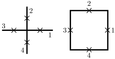
(b)

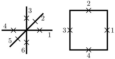
(c)

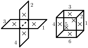
Figure 12: Examples of hypercubic stars and plaquettes for arrays of quantum wires of types (a) (2,1), (b) (3,1), and (c) (3,2). Black crosses represent wires extending perpendicular to all principal directions of the respective hypercubic lattices. The numbers label generalized cardinal directions $C^{\,}_{\mathrm{s}}$ and $C^{\,}_{\mathrm{p}}$ defined in Eqs. (86b) and (87b).

With the hypercubic array of quantum wires defined in this way, we now define hypercubic analogs of stars and plaquettes. Examples of these hypercubic stars and plaquettes are shown in Fig. 12.

Hypercubic “stars” $s$ are centered on each $k^{\,}_{\mathrm{s}}$-cell of the $d$-dimensional lattice with

$$k^{\,}_{\mathrm{s}}\,\raisebox{0.85pt}{.}\raisebox{2.85pt}{.}\!\!=\,k^{\,}_{0}-1.$$ (86a)

They consist of the $$2[d-(k^{\,}_{0}-1)] k^{\,}_{0} (k^{\,}_{0}-1) s 2[d-(k^{\,}_{0}-1)] s$$ nearest-neighbor -cells (and the wires centered on these cells) that border the -cell . (See Fig. 12 for examples.) We label the quantum wires belonging to a hypercubic star by the generalized cardinal direction

$$C^{\,}_{\mathrm{s}}\,\raisebox{0.85pt}{.}\raisebox{2.85pt}{.}\!\!=\,1,\dots,2[d-(k^{\,}_{0}-1)].$$ (86b)

There are

$$N^{\,}_{\mathrm{s}} =\binom{d}{k^{\,}_{0}-1}\,N$$ (86c)

such hypercubic stars in the array of wires labeled by $$(d,k^{\,}_{0})$$.

Hypercubic “plaquettes” $p$ are centered on each $k^{\,}_{\mathrm{p}}$-cell of the $d$-dimensional lattice with

$$k^{\,}_{\mathrm{p}}\,\raisebox{0.85pt}{.}\raisebox{2.85pt}{.}\!\!=\,k^{\,}_{0}+1.$$ (87a)

They consist of the $$2(k^{\,}_{0}+1) k^{\,}_{0} (k^{\,}_{0}+1) p 2(k^{\,}_{0}+1) p$$ nearest-neighbor -cells that border the -cell . (See Fig. 12 for examples.) We label the quantum wires belonging to a hypercubic plaquette by the generalized cardinal direction

$$C^{\,}_{\mathrm{p}}\,\raisebox{0.85pt}{.}\raisebox{2.85pt}{.}\!\!=\,1,\dots,2(k^{\,}_{0}+1).$$ (87b)

There are

$$N^{\,}_{\mathrm{p}} =\binom{d}{k^{\,}_{0}+1}\,N$$ (87c)

such hypercubic plaquettes in the array of wires labeled by $$(d,k^{\,}_{0})$$.

For the square array of quantum wires studied in Sec. II, which has $d=2$ and $k^{\,}_{0}=1$, the generalized cardinalities $C^{\,}_{\mathrm{s}}$ and $C^{\,}_{\mathrm{p}}$ each take values $1,\dots,4$. We identify these with the traditional cardinal directions $C=N,W,S,E$ used in Sec. II.

Note that the substitution $k^{\,}_{0}\to d-k^{\,}_{0}$ exchanges $d-(k^{\,}_{0}-1)\leftrightarrow k^{\,}_{0}+1$. Consequently, the hypercubic array of quantum wires labeled by the pair $(d,k^{\,}_{0})$ is dual to the array labeled by the pair $(d,d-k^{\,}_{0})$, in the sense that the stars of the former are the plaquettes of the latter, and the plaquettes of the former are the stars of the latter. In even dimensions $d$, the hypercubic array of wires labeled by $(d,d/2)$ is therefore self-dual. Consequently, modulo dualities, there is only one such array for $d=3$, as the pairs labeled by $(3,1)$ and $(3,2)$ are dual to one another. The first case where there are multiple hypercubic arrays of quantum wires is therefore $d=4$, which has the dual arrays $(4,1)$ and $(4,3)$, and one self-dual array $(4,2)$.

III.2 Generalizing the results of Sec. II.2

We now turn to the problem of choosing a compatible set of tunneling vectors to gap the bulk of an array of $N^{\,}_{\mathrm{w}}$ quantum wires like those defined in Sec. III.1. As in Sec. II.2, the starting point is an array of decoupled quantum wires described by the quadratic Lagrangian $\hat{L}^{\,}_{0}$ defined in Eq. (1), except that the matrices $\mathcal{K}$ and $\mathcal{V}$ are now of dimension $2MN^{\,}_{\mathrm{w}}$, and the vector of scalar fields

$$\begin{split}\hat{\Phi}(t,z)&\,\raisebox{0.85pt}{.}\raisebox{2.85pt}{.}\!\!=\,\Big{(}\hat{\phi}^{\,}_{1,1}(t,z)\ \dots\ \hat{\phi}^{\,}_{1,2M}(t,z)\mid\\ &\qquad\dots\mid\hat{\phi}^{\,}_{N^{\,}_{\mathrm{w}},1}(t,z)\ \dots\ \hat{\phi}^{\,}_{N^{\,}_{\mathrm{w}},2M}(t,z)\Big{)}^{\mathsf{T}}.\end{split}$$ (88)

This reflects that the quantum wires are now placed on the elementary $k^{\,}_{0}$ cells of a $d$-dimensional hypercubic lattice embedded in $D=d+1$-dimensional Euclidean space. We then add to the free theory the interaction terms $\hat{L}^{\,}_{\{\mathcal{T}\}}$ given in Eq. (7), and set ourselves the challenge of finding a set of $MN^{\,}_{\mathrm{w}}$ tunneling vectors $\mathcal{T}$ satisfying the Haldane criterion (11). We also demand that these tunneling vectors respect some set of symmetries—here, we will enforce only charge conservation [Eq. (10a)], but others, such as TRS or particle-hole symmetry (see Ref. Neupert et al., 2014), may also be relevant. If we can find such a set of tunneling vectors, then, in the strong-coupling limit, $U^{\,}_{\mathcal{T}}\to\infty$ for all $\mathcal{T}$, the array of wires acquires a gap.

As in Sec. II, we reserve the Greek index $\alpha=1,\ldots,2M$ for labeling the bosonic fields within each wire. We reserve the Latin index $j=1,\ldots,N^{\,}_{\mathrm{w}}$ for labeling the wires. A component of the vector of scalar fields $\hat{\Phi}(t,z)$ is then $\hat{\phi}^{\,}_{j,\alpha}(t,z)$.

We claim that the following set of $M\,N^{\,}_{\mathrm{s}}$ integer-valued vectors of dimension $2MN^{\,}_{\mathrm{w}}$,

$$(\mathcal{T}^{(\texttt{j})}_{s})^{\,}_{j,\alpha}\,\raisebox{0.85pt}{.}\raisebox{2.85pt}{.}\!\!=\,v^{(\texttt{j})}_{\alpha}\sum^{d-(k^{\,}_{0}-1)}_{C^{\,}_{\mathrm{s}}=1}\Big{(}\delta^{\,}_{j,s^{\,}_{C^{\,}_{\mathrm{s}}}}\!-\,\delta^{\,}_{j,s^{\,}_{C^{\,}_{\mathrm{s}}+d-(k^{\,}_{0}-1)}}\Big{)},$$ (89a)

and the following set of $$M\,N^{\,}_{\mathrm{p}} 2MN^{\,}_{\mathrm{w}}$$ integer-valued vectors of dimension ,

$$\begin{split}(\mathcal{T}^{(\texttt{j})}_{p})^{\,}_{j,\alpha}&\,\raisebox{0.85pt}{.}\raisebox{2.85pt}{.}\!\!=\,-w^{(\texttt{j})}_{\alpha}\sum^{k^{\,}_{0}}_{C^{\,}_{\mathrm{p}}=1}\Big{(}\delta^{\,}_{j,p^{\,}_{C^{\,}_{\mathrm{p}}}}\!-\,\delta^{\,}_{j,p^{\,}_{C^{\,}_{\mathrm{p}}+k^{\,}_{0}+1}}\Big{)}\\ &\qquad\qquad+w^{(\texttt{j})}_{\alpha}\Big{(}\delta^{\,}_{j,p^{\,}_{k^{\,}_{0}+1}}\!-\,\delta^{\,}_{j,p^{\,}_{2(k^{\,}_{0}+1)}}\Big{)},\end{split}$$ (89b)

does the job, so long as the criteria (17) are satisfied. Here, $v^{(\texttt{j})}$ and $w^{(\texttt{j})}$ are $2M$-dimensional vectors that specify the linear combinations of the fields $\hat{\phi}^{\,}_{j,\alpha}$ in each wire $j$ that enter the cosine terms associated with the tunneling vectors $\mathcal{T}^{(\texttt{j})}_{s}$ and $\mathcal{T}^{(\texttt{j})}_{p}$, respectively. (Their meaning is thus identical to the vectors of the same names presented in Sec. II.2.) Stars and plaquettes are themselves labeled by the indices $s=1,\ldots,N^{\,}_{\mathrm{s}}$ and $p=1,\ldots,N^{\,}_{\mathrm{p}}$, respectively. The teletype index $\texttt{j}=1,\dots,M$ labels $M$ “flavors” of stars and plaquettes. These flavors are necessary, as they were in Sec. II.2, to produce a number of tunneling vectors that is sufficient to gap out all $2M$ gapless degrees of freedom in each wire. (More on counting gapless degrees of freedom in a moment.)

The tunneling vectors defined in Eqs. (89) conserve charge in the sense of Eq. (10a) for any $2M\,N^{\,}_{\mathrm{w}}$-dimensional charge vector $\mathcal{Q}=(Q\mid Q\mid\dots\mid Q)^{\mathsf{T}}$ [recall Eq. (1f)]. To see that this is the case, it suffices to note that the vectors $v^{(\texttt{j})}$ and $w^{(\texttt{j})}$ each enter their respective tunneling vectors with an equal number of $+$ and $-$ signs. Consequently, no matter the values of $Q^{\mathsf{T}}v^{(\texttt{j})}$ and $Q^{\mathsf{T}}w^{(\texttt{j})}$, this value is added and subtracted an equal number of times. This fact provides a direct parallel with the construction of Sec. II.2, where the tunneling vectors defined in Eqs. (13) conserve charge independently of the form of the $2M$-dimensional charge vector $Q$ of a single wire.

One can verify that the tunneling vectors (89) satisfy the Haldane criterion (11), as expressed in Eqs. (12), if Eqs. (17) hold, with the help of the following observations. First, note that these tunneling vectors coincide with the tunneling vectors (13) defined in Sec. II.2 in the case $(d,k^{\,}_{0})=(2,1)$, which was studied there. Second, note that Eqs. (12a) and (12b) hold if Eqs. (17) hold. Third, recall that if a hypercubic star $s$ and a hypercubic plaquette $p$ overlap with one another, then they share two wires (see Ref. Mazáč and Hamma (2012)). With this in mind, we can see that Eq. (12c) holds for the tunneling vectors (89) by focusing on the case where the star $s$ and plaquette $p$ overlap [since Eq. (12c) holds trivially otherwise]. This can be seen by looking only at the parts of the tunneling vectors (89) that lie in the crystal plane that contains the two wires in the union of $s$ and $p$. The projection of the tunneling vectors (89) into this plane is, by construction, precisely the set of tunneling vectors (13) defined in Sec. II.2 (but specialized from the outset to the case $v^{(\texttt{j})}_{1}=v^{(\texttt{j})}_{2}=v^{(\texttt{j})}$ and $w^{(\texttt{j})}_{1}=w^{(\texttt{j})}_{2}=w^{(\texttt{j})}$). Equation (12c) then follows.

Having seen that the tunneling vectors (89) encode charge-conserving many-body interactions and are Haldane-compatible, one must next determine that these tunneling vectors are sufficient in number to gap out all $2M\,N^{\,}_{\mathrm{w}}$ gapless degrees of freedom in the array of quantum wires.

Recall from the discussion in Sec. II.2 that, in order to produce a gapped array of quantum wires, one requires $M\,N^{\,}_{\mathrm{w}}$ admissible tunneling vectors (since each admissible tunneling vector gaps out two gapless modes). It is therefore necessary to compare the number of tunneling vectors in the set defined in Eqs. (89) with the number of wires in the array. From Eqs. (85), (86c), and (87c), we see that

$$N^{\,}_{\mathrm{s}}+N^{\,}_{\mathrm{p}}\geq N^{\,}_{\mathrm{w}},$$ (90)

with strict equality occurring in arrays of type $(2,1)$, which were studied in Sec. II.

In cases where Eq. (90) is an inequality, the question arises of how one can account for the extra gapless degrees of freedom. In this case, we can appeal to intuition developed from the study of toric codes in arbitrary dimensions (see, e.g., Ref. Mazáč and Hamma (2012)). In a toric code on a hypercubic lattice of type $(d,k^{\,}_{0})$ (with spin-1/2 degrees of freedom, rather than quantum wires, placed on the centers of elementary $k^{\,}_{0}$-cells of the $d$-dimensional hypercubic lattice), the same inequality shown in Eq. (90) holds (with the number of spins now given by $N^{\,}_{\mathrm{w}}$). However, in the toric code of type $(d,k^{\,}_{0})$, there are precisely $N^{\,}_{\mathrm{s}}+N^{\,}_{\mathrm{p}}-N^{\,}_{\mathrm{w}}$ local constraints that account for the discrepancy between the number of spin-1/2 degrees of freedom and the total number of stars and plaquettes. For example, in the three-dimensional toric code labeled by $(3,1)$, the product of all two-dimensional plaquettes on the surface of a cubic unit cell of the lattice is equal to 1. This introduces $N$ local constraints, since there are $N$ such cubes in the lattice. From Eqs. (85), (86c), and $\eqref{N plaquette}$, we have $N^{\,}_{\mathrm{w}}=3N$, $N^{\,}_{\mathrm{s}}=N$, and $N^{\,}_{\mathrm{p}}=3N$. The $N$ local constraints thus account for the $N^{\,}_{\mathrm{s}}+N^{\,}_{\mathrm{p}}-N^{\,}_{\mathrm{w}}=N$ missing degrees of freedom. (Note that, similarly to the toric code, there are also further nonlocal constraints among the tunneling vectors. These are important for determining the topological ground-state degeneracy.)

In the corresponding array of coupled quantum wires, the local constraints described above translate into linear dependencies within the sets $\{\mathcal{T}^{(\texttt{j})}_{s}\}$ and $\{\mathcal{T}^{(\texttt{j})}_{p}\}$ for each flavor $\texttt{j}=1,\dots,M$. In other words, if there are $N^{\,}_{\mathrm{s}}+N^{\,}_{\mathrm{p}}>N^{\,}_{\mathrm{w}}$ tunneling vectors for each of the $M$ flavors of hypercubic stars and plaquettes, then precisely $N^{\,}_{\mathrm{s}}+N^{\,}_{\mathrm{p}}-N^{\,}_{\mathrm{w}}$ of these tunneling vectors are linearly dependent. This ensures that an array of quantum wires with $2M\,N^{\,}_{\mathrm{w}}$ gapless degrees of freedom has precisely $MN^{\,}_{\mathrm{w}}$ linearly independent tunneling vectors of the form (89). We will provide an example of this linear dependence in the next section, where we present an array of coupled wires of type $(3,1)$.

Once an appropriate set of interactions encoded by the tunneling vectors $\mathcal{T}^{(\texttt{j})}_{s}$ and $\mathcal{T}^{(\texttt{j})}_{p}$ has been chosen, for example by the construction outlined in this section, the $d$-dimensional array of quantum wires becomes a gapped $D\equiv(d+1)$-dimensional state of matter. The excitations of this state of matter, as well as their (possibly) fractional quantum numbers and any associated topological degeneracy on the $D$-torus, can be studied using the methods of Sec. II.3. As in that section, one identifies excitations with solitons in the pinned fields $\mathcal{T}^{(\texttt{j})\mathsf{T}}_{s}\,\mathcal{K}\Phi$ and $\mathcal{T}^{(\texttt{j})\mathsf{T}}_{p}\,\mathcal{K}\Phi$. Depending on the values of $d$ and $k^{\,}_{0}$ that characterize the underlying hypercubic lattice, these defects will be pointlike, stringlike, or membranelike in nature. When periodic boundary conditions are imposed, propagating these pointlike, stringlike, or membranelike defects across the entire system defines nonlocal string and/or membrane operators, whose algebra can be used to determine the presence or absence of topological order in the strongly-interacting, $D$-dimensional, gapped phase of matter.

(a)

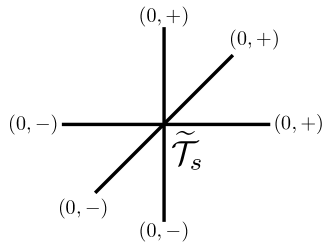
(b)

Figure 13: Pictorial representations of the tunneling vectors (a) $\tilde{\mathcal{T}}^{\,}_{s}$ and (b) $\tilde{\mathcal{T}}^{\,}_{p}$, defined in Eqs. (89), for the array of quantum wires of type $(3,1)$. As in Fig. 10, they are built using the vectors $\tilde{v}$ and $\tilde{w}$ defined in Eqs. (62).

(a)

(b)

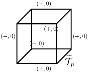
Figure 14: Pictorial representations of the tunneling vectors (a) $\tilde{\mathcal{T}}^{\,}_{s}$ and (b) $\tilde{\mathcal{T}}^{\,}_{p}$, defined in Eqs. (89), for the array of quantum wires of type $(3,2)$. As in Figs. 10 and 13, they are built using the vectors $\tilde{v}$ and $\tilde{w}$ defined in Eqs. (62).

III.3 Example: $\mathbb{Z}^{\,}_{m}$ topological order in four-dimensional space from coupled wires

In this section, we provide a concrete example of how the construction of Abelian topological states of matter outlined in Sec. II can be generalized to higher dimensions. In particular, we construct four-dimensional analogs of the $\mathbb{Z}^{\,}_{m}$ topological states of matter explored in Sec. II.4.

Our starting point is a cubic array of quantum wires of type $(3,1)$, with periodic boundary conditions imposed in all four spatial directions from the outset. [We will also consider in parallel a related realization of $\mathbb{Z}^{\,}_{m}$ topological order that starts from the dual array of type $(3,2)$.] This array has the stars and plaquettes shown in Fig. 12(b). We use the coordinates $x,y,$ and $z$ to label directions within the cubic array, and $w$ to label the coordinate along each wire.

The initial Lagrangian of the system of decoupled wires is precisely the one described in Sec. II.4.1 for a system with $N^{\,}_{\mathrm{w}}=3N$ quantum wires, each containing $2M=2$ gapless degrees of freedom. In particular, starting from the free Lagrangian (1) with

$$\mathcal{K}\,\raisebox{0.85pt}{.}\raisebox{2.85pt}{.}\!\!=\,\mathbbm{1}^{\,}_{3N}\otimes K^{\,}_{\mathrm{b}},$$ (91)

where the bosonic $K$-matrix $K^{\,}_{\mathrm{b}}$ is defined in Eq. (3b), we perform the change of basis (18) with the $2\times 2$ matrix $W$ given by Eq. (57a). In this way, we obtain a theory of decoupled wires with the $K$-matrix $\tilde{K}_{m}$ given in Eq. (57b). (It is worth pointing out here that this initial phase of the construction is, as we have seen in this paragraph, independent of the dimensionality of the array of quantum wires.)

Next, we couple the wires with the many-body interactions $\tilde{\hat{L}}^{\,}_{\{\tilde{\mathcal{T}}\}}$, defined as in Eq. (7), for tunneling vectors $\tilde{\mathcal{T}}$ given by Eqs. (89) with the two-dimensional vectors $\tilde{v}$ and $\tilde{w}$ defined in Eqs. (62). These tunneling vectors are shown in Fig. 13 for the array of type (3,1), and in Fig. 14 for the array of type (3,2). Using these pictorial representations of the tunneling vectors, one can verify that both sets of tunneling vectors satisfy the Haldane criterion (11) with the $K$-matrix (57b), as desired. Furthermore, it is straightforward to check that these tunneling vectors are charge-conserving. They satisfy Eq. (10a) for any charge vector $\mathcal{Q}$ of the form (1f).

We now verify that the tunneling vectors depicted in Figs. 13 and 14 are sufficient in number to produce a gapped four-dimensional state of matter. We will focus here on the array of coupled wires of type $(3,1)$, since the counting is identical for the array of type $(3,2)$. To do this, we recall from Sec. III.2 that the total number of tunneling vectors is given by $N^{\,}_{\mathrm{s}}+N^{\,}_{\mathrm{p}}=4N$, while the total number of gapless degrees of freedom in the array of decoupled quantum wires is $2N^{\,}_{\mathrm{w}}=6N$. Since only $3N$ linearly independent tunneling vectors are necessary to produce a fully gapped state of matter, there must be a set of local constraints that removes $N$ tunneling vectors from the Haldane set $\mathbb{H}$. One can check that this is indeed the case, as the set of six tunneling vectors $\mathcal{T}^{\,}_{p}$ lining the surface of any cubic cell of the three-dimensional cubic lattice are linearly dependent. One can verify this statement by computing the Gram matrix with elements

$$G^{\,}_{pp^{\prime}}\,\raisebox{0.85pt}{.}\raisebox{2.85pt}{.}\!\!=\,\mathcal{T}^{\mathsf{T}}_{p}\,\mathcal{T}^{\,}_{p^{\prime}},$$ (92)

where the plaquettes $p$ and $p^{\prime}$ border such a cubic cell. One finds (see Fig. 15 for guidance) that

$$G=\begin{pmatrix}4&-1&-1&+1&+1&0\\ -1&4&-1&0&+1&+1\\ -1&-1&4&+1&0&+1\\ +1&0&+1&4&-1&-1\\ +1&+1&0&-1&4&-1\\ 0&+1&+1&-1&-1&4\end{pmatrix},$$ (93)

which has vanishing determinant, indicating that this set of six tunneling vectors is linearly dependent. Since the cubic lattice contains exactly $N$ such cubes when periodic boundary conditions are imposed, there are $N$ linearly dependent vectors that can be removed from the Haldane set $\mathbb{H}$. [Note that a similar set of local constraints for stars holds in the case of the array of wires of type (3,2). This is due to the duality between hypercubic arrays of types $(d,k^{\,}_{0})$ and $(d,d-k^{\,}_{0})$ mentioned in Sec. III.1.]

Figure 15: Pictorial representation of the six plaquette-centered tunneling vectors $\mathcal{T}^{\,}_{p}$ surrounding a cubic cell of the array of quantum wires labeled by (3,1). (Folding sides $2,\dots,5$ upwards out of the page and placing side $6$ on top constructs the cubic cell.) The numbers $1,\dots,6$ label these tunneling vectors in the order in which they appear in the Gram matrix $G$ in Eq. (93). The signs $\pm$ indicate whether a $\pm 1$ appears in the tunneling vector associated with that link.

On the basis of the above arguments, we conclude that the cubic arrays of types $(3,1)$ and $(3,2)$ both yield fully gapped, four-dimensional states of matter when periodic boundary conditions are imposed. The excitations of both states of matter can be studied according to the methodology laid out in Sec. II.3, and by example in Sec. II.4.2. As in that section, the building blocks of excitations in the array of coupled wires are the local operators

$$\hat{S}^{{\dagger}}_{s^{\,}_{C^{\,}_{\mathrm{s}}}}(w)\,\raisebox{0.85pt}{.}\raisebox{2.85pt}{.}\!\!=\,\exp\left(-\mathrm{i}\,\tilde{\hat{\phi}}^{\,}_{s^{\,}_{C^{\,}_{\mathrm{s}}},2}(w)\right)$$ (94a)

and

$$\hat{P}^{{\dagger}}_{p^{\,}_{C^{\,}_{\mathrm{p}}}}(w)\,\raisebox{0.85pt}{.}\raisebox{2.85pt}{.}\!\!=\,\exp\left(+\mathrm{i}\,\tilde{\hat{\phi}}^{\,}_{p^{\,}_{C^{\,}_{\mathrm{p}}},1}(w)\right),$$ (94b)

and the bilocal operators

$$\begin{split}\hat{S}^{{\dagger}}_{s^{\,}_{C^{\,}_{\mathrm{s}}}}(w^{\,}_{1},w^{\,}_{2})&\,\raisebox{0.85pt}{.}\raisebox{2.85pt}{.}\!\!=\,\hat{S}^{{\dagger}}_{s^{\,}_{C^{\,}_{\mathrm{s}}}}(w^{\,}_{2})\,\hat{S}^{\phantom{{\dagger}}}_{s^{\,}_{C^{\,}_{\mathrm{s}}}}(w^{\,}_{1})\\ &=\exp\bigg{(}-\mathrm{i}\,\int\limits^{w^{\,}_{2}}_{w^{\,}_{1}}\mathrm{d}w\ \partial^{\,}_{w}\tilde{\hat{\phi}}^{\,}_{s^{\,}_{C^{\,}_{\mathrm{s}}},2}(w)\bigg{)},\end{split}$$ (95a)

and

$$\begin{split}\hat{P}^{{\dagger}}_{p^{\,}_{C^{\,}_{\mathrm{p}}}}(w^{\,}_{1},w^{\,}_{2})&\,\raisebox{0.85pt}{.}\raisebox{2.85pt}{.}\!\!=\,\hat{P}^{{\dagger}}_{p^{\,}_{C^{\,}_{\mathrm{p}}}}(w^{\,}_{2})\,\hat{P}^{\phantom{{\dagger}}}_{p^{\,}_{C^{\,}_{\mathrm{p}}}}(w^{\,}_{1})\\ &=\exp\bigg{(}+\mathrm{i}\,\int\limits^{w^{\,}_{2}}_{w^{\,}_{1}}\mathrm{d}w\ \partial^{\,}_{w}\tilde{\hat{\phi}}^{\,}_{p^{\,}_{C^{\,}_{\mathrm{p}}},1}(w)\bigg{)}.\end{split}$$ (95b)

Here, we recall that the coordinate along each wire is now labeled by $w$, and that the indices $C^{\,}_{\mathrm{s}}=1,\dots,2[d-(k^{\,}_{0}-1)]$ and $C^{\,}_{\mathrm{p}}\,\raisebox{0.85pt}{.}\raisebox{2.85pt}{.}\!\!=\,1,\dots,2(k^{\,}_{0}+1)$ label the generalized cardinal directions associated with each star or plaquette.

The effects of the operators defined in Eqs. (94) and (95) on the pinned fields $\mathcal{T}^{\mathsf{T}}_{s}\,\tilde{\mathcal{K}}\,\tilde{\Phi}$ and $\mathcal{T}^{\mathsf{T}}_{p}\,\tilde{\mathcal{K}}\,\tilde{\Phi}$ can be computed analogously to Eqs. (32), (35), (33), and (36). As shown there, these operators give rise to the excitations of the array of coupled wires. One can deduce whether the excitations created and propagated by these operators are pointlike, stringlike, or membranelike by first acting with one of these operators on a single link. This creates some number of defective stars or plaquettes (depending on the coordination number of that link and whether or not the operator acts along the direction of the wire). From there, one can grow a surface with excitations on its boundary by attempting to heal all defects created in this way with further applications of the operators defined in Eqs. (94) or (95). Processes analogous to this one are shown in Figs. 4 and 5 for the array of type $(2,1)$ studied in Sec. II. As in Sec. II.4.2, the electric charge associated with these defects can be computed as in Eq. (64). The excitations of the array of type $(3,1)$ differ in character from those of the array of type $(3,2)$, as we shall now see.

The excitations of the array of type $(3,1)$ can be pointlike, linelike, or membranelike in nature. To see this, note that applying the operator $\hat{S}^{{\dagger}}_{s^{\,}_{C^{\,}_{\mathrm{s}}}}(w)$ in the wire labeled by $s^{\,}_{C^{\,}_{\mathrm{s}}}$ creates two defective stars, as there are two stars bordering each link in the array of wires. These defective stars can be propagated away from one another, much as in Fig. 4, by further applications of the operator $\hat{S}^{{\dagger}}_{s^{\,}_{C^{\,}_{\mathrm{s}}}}(w)$. Consequently, we may view the defective stars as pointlike excitations with electric charge $\pm 2/m$ [recall Eq. (64)], connected by a “string” of vertex operators. One can also construct linelike excitations, for example by acting instead with the bilocal operator $\hat{S}^{{\dagger}}_{s^{\,}_{C^{\,}_{\mathrm{s}}}}(w^{\,}_{1},w^{\,}_{2})$, similarly to Fig. 5(a)-(b).

On the other hand, suppose that one applies the operator $\hat{P}^{{\dagger}}_{p^{\,}_{C^{\,}_{\mathrm{p}}}}(w)$ in the wire labeled by $p^{\,}_{C^{\,}_{\mathrm{p}}}$. In this case, one creates four defective plaquettes, as each link is shared by four plaquettes. Attempting to heal these defects by subsequent applications of the operator $\hat{P}^{{\dagger}}_{p^{\,}_{C^{\,}_{\mathrm{p}}}}(w)$ leads to a two-dimensional membrane of vertex operators with linelike defects on its boundary, much like in Fig. 5(c)-(d). Furthermore, one can also create a 3-brane of vertex operators with two-dimensional membranelike excitations on its terminating surfaces, by applying the operator $\hat{P}^{{\dagger}}_{p^{\,}_{C^{\,}_{\mathrm{p}}}}(w^{\,}_{1},w^{\,}_{2})$ instead of $\hat{P}^{{\dagger}}_{p^{\,}_{C^{\,}_{\mathrm{p}}}}(w)$.

A similar set of excitations can be constructed for the case of the array of type $(3,2)$. The only difference is that, in this case, the vertex operators associated with stars naturally form membranes, similarly to the plaquettes in the array of type $(3,1)$. This makes sense in light of the duality between these two arrays of quantum wires, which exchanges stars and plaquettes, and therefore also necessarily exchanges star and plaquette defects.

We now demonstrate that the gapped four-dimensional phases of matter associated with the cubic arrays of types $(3,1)$ and $(3,2)$ are topologically ordered. calculating the minimal topological ground-state degeneracy on the four-torus,

$$\mathbb{T}^{4}\equiv S^{1}\times S^{1}\times S^{1}\times S^{1},$$ (96)

by generalizing the analysis of Sec. II.3.6, i.e., by presenting the algebra of nonlocal operators from which the degeneracy is derived. We focus on the array of type $(3,1)$, as the degeneracy of the array of type $(3,2)$ is the same by the duality discussed in Sec. III.1. In both cases, the origin of the multidimensionality of the ground-state manifold is the nontrivial (for $m>1$) equal-time algebra

$$\begin{split}\hat{S}^{{\dagger}}_{j}(w)\,\hat{P}^{{\dagger}}_{j}(0,L)&=\hat{P}^{{\dagger}}_{j}(0,L)\,\hat{S}^{{\dagger}}_{j}(w)\,e^{-\mathrm{i}\,2\pi/m},\\ \hat{P}^{{\dagger}}_{j}(w)\,\hat{S}^{{\dagger}}_{j}(0,L)&=\hat{S}^{{\dagger}}_{j}(0,L)\,\hat{P}^{{\dagger}}_{j}(w)\,e^{+\mathrm{i}\,2\pi/m},\end{split}$$ (97)

which holds independently of dimensionality or lattice geometry as it is a property of operators defined in a single wire. Consequently, there is no obstruction to repeating this analysis for any hypercubic array of type $(d,k^{\,}_{0})$.

The ground state degeneracy on $\mathbb{T}^{4}$ of the array of type $(3,1)$ is encoded in the algebra of the nonlocal operators

$$\hat{\mathcal{O}}^{\,}_{P,\Omega^{\,}_{\hat{x}\hat{y}\hat{z}}}(w)\,\raisebox{0.85pt}{.}\raisebox{2.85pt}{.}\!\!=\,\prod_{p^{\,}_{C^{\,}_{\mathrm{p}}}\in\Omega^{\,}_{\hat{x}\hat{y}\hat{z}}}P^{{\dagger}}_{p^{\,}_{C^{\,}_{\mathrm{p}}}}(w),$$ (98a)

$$\hat{\mathcal{O}}^{\,}_{P,\Omega^{\,}_{\hat{x}\hat{y}\hat{w}}}\,\raisebox{0.85pt}{.}\raisebox{2.85pt}{.}\!\!=\,\prod_{p^{\,}_{C^{\,}_{\mathrm{p}}}\in\Omega^{\,}_{\hat{x}\hat{y}}}P^{{\dagger}}_{p^{\,}_{C^{\,}_{\mathrm{p}}}}(0,L),$$ (98b)

$$\hat{\mathcal{O}}^{\,}_{P,\Omega^{\,}_{\hat{x}\hat{z}\hat{w}}}\,\raisebox{0.85pt}{.}\raisebox{2.85pt}{.}\!\!=\,\prod_{p^{\,}_{C^{\,}_{\mathrm{p}}}\in\Omega^{\,}_{\hat{x}\hat{z}}}P^{{\dagger}}_{p^{\,}_{C^{\,}_{\mathrm{p}}}}(0,L),$$ (98c)

$$\hat{\mathcal{O}}^{\,}_{P,\Omega^{\,}_{\hat{y}\hat{z}\hat{w}}}\,\raisebox{0.85pt}{.}\raisebox{2.85pt}{.}\!\!=\,\prod_{p^{\,}_{C^{\,}_{\mathrm{p}}}\in\Omega^{\,}_{\hat{y}\hat{z}}}P^{{\dagger}}_{p^{\,}_{C^{\,}_{\mathrm{p}}}}(0,L),$$ (98d)

which act along 3-branes, and

$$\hat{\mathcal{O}}^{\,}_{S,\Gamma^{\,}_{x}}(w)\,\raisebox{0.85pt}{.}\raisebox{2.85pt}{.}\!\!=\,\prod_{s^{\,}_{C^{\,}_{\mathrm{s}}}\in\Gamma^{\,}_{x}}\hat{S}^{{\dagger}}_{s^{\,}_{C^{\,}_{\mathrm{s}}}}(w),$$ (98e)

$$\hat{\mathcal{O}}^{\,}_{S,\Gamma^{\,}_{y}}(w)\,\raisebox{0.85pt}{.}\raisebox{2.85pt}{.}\!\!=\,\prod_{s^{\,}_{C^{\,}_{\mathrm{s}}}\in\Gamma^{\,}_{y}}\hat{S}^{{\dagger}}_{s^{\,}_{C^{\,}_{\mathrm{s}}}}(w),$$ (98f)

$$\hat{\mathcal{O}}^{\,}_{S,\Gamma^{\,}_{z}}(w)\,\raisebox{0.85pt}{.}\raisebox{2.85pt}{.}\!\!=\,\prod_{s^{\,}_{C^{\,}_{\mathrm{s}}}\in\Gamma^{\,}_{z}}\hat{S}^{{\dagger}}_{s^{\,}_{C^{\,}_{\mathrm{s}}}}(w),$$ (98g)

$$\hat{\mathcal{O}}^{\,}_{S,\Gamma^{\,}_{w}}\,\raisebox{0.85pt}{.}\raisebox{2.85pt}{.}\!\!=\,\hat{S}^{{\dagger}}_{s^{\,}_{0}}(0,L),$$ (98h)

which act along strings. The volume $\Omega^{\,}_{\hat{x}\hat{y}\hat{z}}$, the surface $\Omega^{\,}_{\hat{x}\hat{y}}$, the line $\Gamma^{\,}_{x}$, etc. are defined analogously to their counterparts in Sec. II.3.6. Their algebra is found to be

$$\hat{\mathcal{O}}^{\,}_{P,\Omega^{\,}_{\hat{x}\hat{y}\hat{z}}}(w)\,\hat{\mathcal{O}}^{\,}_{S,\Gamma^{\,}_{w}} =\hat{\mathcal{O}}^{\,}_{S,\Gamma^{\,}_{w}}\,\hat{\mathcal{O}}^{\,}_{P,\Omega^{\,}_{\hat{x}\hat{y}\hat{z}}}(w)\,e^{+\mathrm{i}\,2\pi/m},$$ (99a)

$$\hat{\mathcal{O}}^{\,}_{P,\Omega^{\,}_{\hat{x}\hat{y}\hat{w}}}\,\hat{\mathcal{O}}^{\,}_{S,\Gamma^{\,}_{z}}(w) =\hat{\mathcal{O}}^{\,}_{S,\Gamma^{\,}_{z}}(w)\,\hat{\mathcal{O}}^{\,}_{P,\Omega^{\,}_{\hat{x}\hat{y}\hat{w}}}\,e^{-\mathrm{i}\,2\pi/m},$$ (99b)

$$\hat{\mathcal{O}}^{\,}_{P,\Omega^{\,}_{\hat{x}\hat{z}\hat{w}}}\,\hat{\mathcal{O}}^{\,}_{S,\Gamma^{\,}_{y}}(w) =\hat{\mathcal{O}}^{\,}_{S,\Gamma^{\,}_{y}}(w)\,\hat{\mathcal{O}}^{\,}_{P,\Omega^{\,}_{\hat{x}\hat{z}\hat{w}}}\,e^{-\mathrm{i}\,2\pi/m},$$ (99c)

$$\hat{\mathcal{O}}^{\,}_{P,\Omega^{\,}_{\hat{y}\hat{z}\hat{w}}}\,\hat{\mathcal{O}}^{\,}_{S,\Gamma^{\,}_{x}}(w) =\hat{\mathcal{O}}^{\,}_{S,\Gamma^{\,}_{x}}(w)\,\hat{\mathcal{O}}^{\,}_{P,\Omega^{\,}_{\hat{y}\hat{z}\hat{w}}}\,e^{-\mathrm{i}\,2\pi/m},$$ (99d)

where we have made extensive use of Eq. (97). Similarly to what was found in Sec. II.4.3, each line of the above algebra is independent from (i.e., commutes with) the others, and contributes an $m$-fold topological degeneracy. We conclude that the total topological degeneracy on the four-torus of this state of matter is

$$D^{\,}_{\mathbb{T}^{4}}=m^{4}.$$ (100)

For $m=2$, the 16-fold degeneracy coincides with the ground-state degeneracy of the four-dimensional toric code defined on the hypercubic lattice of type $(4,1)$ Mazáč and Hamma (2012). For $m>1$, we have therefore arrived at a state of matter whose low-lying excitations and topological ground-state degeneracy on the four-torus are consistent with a $\mathbb{Z}^{\,}_{m}$-topologically-ordered phase in four spatial dimensions.

From here, one could further generalize the discussion of Sec. II.4.4 in order to enumerate the possible gapped or gapless states of matter on the three-dimensional boundary of the four-dimensional bulk topological phase. Terminating the cubic lattice of type $(3,1)$ in the $y$-direction, say, leads to a surface lattice of type $(2,1)$, i.e., a square lattice with wires on the links. One is then free to impose any single-particle tunneling or many-body interactions one wishes on the surface, so long as these surface terms are Haldane-compatible with the bulk. For example, one could search the space of tunneling vectors like those defined in Sec. II.2 to generate a set of allowed many-body interactions. This method of studying the surface states can be readily generalized to any hypercubic array of quantum wires of type $(d,k^{\,}_{0})$, like those studied in Sec. III, to answer questions about higher-dimensional generalizations of the concept of surface topological order, for example.

The discussion of this section can be generalized to arrays of quantum wires of type $(d,k^{\,}_{0})$ to produce $\mathbb{Z}^{\,}_{m}$-topologically-ordered phases in higher dimensions. Many of these higher-dimensional topological states of matter are particularly interesting in that they exhibit topological order at finite temperature Mazáč and Hamma (2012). The lowest-dimensional $\mathbb{Z}^{\,}_{m}$-topologically-ordered phase exhibiting topological order at finite temperature is the toric code of type (4,2). The discussion of this section demonstrates that one cannot realize a topological state of matter in the universality class of the toric code of type (4,2) starting from an array of quantum wires of type (3,1) or (3,2). This is because both of these arrays yield topological states of matter whose degeneracy is consistent with the toric code of type (4,1) [recall Eq. (100)]. However, this does not preclude the possibility of designing arrays of quantum wires to yield topological states of matter in $D=5$ or greater that have topological order at finite temperature. The detailed study of such phases is beyond the scope of this work, but nevertheless a very interesting problem for future study.

IV Conclusion

In this paper, we have outlined a general strategy for designing Abelian topological phases of matter in $D$ spatial dimensions by coupling an array of quantum wires in $d=D-1$ dimensions. This strategy hinges on the use of counting arguments introduced by Haldane Haldane (1995) to search for a set of compatible many-body interactions that yields a gapped state of matter when the couplings associated with these interactions are taken to infinity. The enumeration of the set of possible interactions, and the determination of their compatibility, is aided by associating each interaction term with one of the generalized stars and plaquettes of a $d$-dimensional hypercubic lattice embedded in $D$-dimensional space. In this sense, the interactions that produce a gapped state of matter are arranged in a manner reminiscent of the commuting projectors in a $d$-dimensional toric code.

We found that many simplifications arise due to this similarity, making these theories analytically tractable much as their forebears in two dimensions. In particular, the excitations of the arrays of coupled wires can be studied thanks in part to analogies with similar excitations in the $d$-dimensional toric code. The fractional charge and statistics of these excitations is readily accessible with standard tools from Abelian bosonization. Furthermore, when periodic boundary conditions are imposed, the topological degeneracy (if any) of the strongly-interacting, gapped, $D$-dimensional state of matter can be determined with these tools. Finally, when the array of coupled wires is defined on a manifold with boundary, the stability of gapless surface states on the $d$-dimensional boundary of the $D$-dimensional topological phase can be addressed conveniently with the same formalism in one less spatial dimension, provided that any single-particle tunnelings or many-body interactions added to the surface are compatible with those in the bulk.

There are many directions for future work in light of these findings. First, it is important to note that the class of many-body interactions introduced in Secs. II.2 and III.2 are not the only ones possible, even when making use of the analogy to $d$-dimensional toric codes; there are many other sets of compatible tunneling vectors that can be associated with the stars and plaquettes of hypercubic lattices. Consequently, it would be instructive to map out the set of all Abelian topological phases possible in three and higher dimensions that are accessible with this approach. Even in three spatial dimensions, there are many possible topological field theories beyond the BF-type theories explored in Sec. II.3.7, such as those studied in Refs. Ye and Gu (2015), Ye (1), and Che (b). It would also be interesting to determine whether other exactly solvable commuting-projector Hamiltonians, besides toric codes, could be used as bases for wire constructions like the ones undertaken in this work, resulting in different classes of topological phases. Second, it would be interesting to study the surface states of these coupled-wire arrays in more detail. In particular, finding a useful way to characterize gapless surfaces by extending the formalism presented in this paper would be a very useful pursuit, as one might ask the question of whether it is possible to find novel non-Fermi liquids or conformal field theories on interacting surfaces of topological phases in three or more dimensions. In this pursuit, it would also be crucial to make contact with existing work on the bulk-boundary correspondence in three dimensions Cho and Moore (2011); Chan et al. (2013); Che (b). Third, it is natural to ask how to extend this formalism to describe non-Abelian topological states of matter. This could be done by investigating the possibility of using non-Abelian, rather than Abelian, bosonization to describe the gapless wires and their couplings to one another, as has been done in Refs. Teo and Kane (2014) and Hua . Fourth, as was hinted at in this work, wire constructions of topological phases in spatial dimensions greater than two could prove useful in the study of surface topological order von Keyserlingk et al. (2013); Vishwanath and Senthil (2013); Wang and Senthil (2013); Wang et al. (2013); Burnell et al. (2014); Chen et al. (2014); Metlitski et al. (2015); Mross et al. (2015). In particular, it may be possible to use non-Abelian bosonization techniques on the surfaces of Abelian topological phases to study non-Abelian surface topological orders in a manner that treats the surface and bulk physics simultaneously.

Appendix A Deconfinement of defects along the direction of a wire

In this Appendix, we demonstrate that a pair of star defects in three dimensions, like the one shown in Fig. 4(b), are deconfined from one another along the $z$-direction, despite the string of vertex operators connecting them. This is because a link in the string, which consists of two vertex operators applied on two legs of a star (see Fig. 4), costs no additional energy if the vertex operators are displaced relative to one another along the $z$-axes of their respective wires. While we focus here on the specfic example of star defects in the $\mathbb{Z}^{\,}_{m}$-topologically-ordered state of matter constructed in Sec. II.4, the same analysis can be adapted to demonstrate that pointlike star and plaquette defects are deconfined in any dimension.

To see that this is the case, let us consider a star $s$ with two $2\pi/m$ solitons on the eastern and western legs. We parameterize these solitons by decomposing the bosonic fields as

$$\begin{split}\tilde{\hat{\phi}}^{\,}_{s^{\,}_{E},1}(z)&=f^{\,}_{\mathrm{sol}}(z-z^{\,}_{E})+\tilde{\hat{\phi}}^{\prime}_{s^{\,}_{E},1}(z),\\ \tilde{\hat{\phi}}^{\,}_{s^{\,}_{W},1}(z)&=f^{\,}_{\mathrm{sol}}(z-z^{\,}_{W})+\tilde{\hat{\phi}}^{\prime}_{s^{\,}_{W},1}(z),\end{split}$$ (A1a)

where the real-valued function

$$f^{\,}_{\mathrm{sol}}(z-z^{\,}_{0}) \,\raisebox{0.85pt}{.}\raisebox{2.85pt}{.}\!\!=\,\frac{\pi}{m}\left[\tanh\left(\frac{z-z^{\,}_{0}}{\xi}\right)+1\right]$$ (A1b)

is a fixed soliton profile centered at $$z^{\,}_{0} \tilde{\hat{\phi}}^{\prime}_{s^{\,}_{C},1}(z) C=N,S,E,W$$, while it is the primed fields () that encode the quantum fluctuations.

On the one hand, if $z^{\,}_{E}=z^{\,}_{W}$, Eq. (65a) dictates that

$$\tilde{\mathcal{T}}^{\mathsf{T}}_{s}\,\tilde{\mathcal{K}}^{\,}_{m}\,\tilde{\hat{\Phi}}(z)=m\left[\tilde{\hat{\phi}}^{\,}_{s^{\,}_{N},1}(z)-\tilde{\hat{\phi}}^{\,}_{s^{\,}_{S},1}(z)+\tilde{\hat{\phi}}^{\prime}_{s^{\,}_{E},1}(z)-\tilde{\hat{\phi}}^{\prime}_{s^{\,}_{W},1}(z)\right]\equiv\tilde{\mathcal{T}}^{\mathsf{T}}_{s}\,\tilde{\mathcal{K}}^{\,}_{m}\,\tilde{\hat{\Phi}}^{\prime}(z).$$ (A2a)

On the other hand, if $$z^{\,}_{E}\neq z^{\,}_{W}$$, Eq. (65a) dictates that

$$\tilde{\mathcal{T}}^{\mathsf{T}}_{s}\,\tilde{\mathcal{K}}^{\,}_{m}\,\tilde{\hat{\Phi}}(z)=m\left[\tilde{\hat{\phi}}^{\,}_{s^{\,}_{N},1}(z)-\tilde{\hat{\phi}}^{\,}_{s^{\,}_{S},1}(z)+\tilde{\hat{\phi}}^{\prime}_{s^{\,}_{E},1}(z)-\tilde{\hat{\phi}}^{\prime}_{s^{\,}_{W},1}(z)+\delta\tilde{\phi}^{\,}_{s}(z)\right],$$ (A2b)

where

$$\delta\tilde{\phi}^{\,}_{s}(z) =\frac{\pi}{m}\left[\tanh\left(\frac{z-z^{\,}_{E}}{\xi}\right)-\tanh\left(\frac{z-z^{\,}_{W}}{\xi}\right)\right].$$ (A2c)

In the limit $\xi\to 0$ (i.e., the limit of perfectly sharp solitons),

$$\delta\tilde{\phi}^{\,}_{s}(z) \longrightarrow\frac{2\pi}{m}\left[\Theta(z-z^{\,}_{E})-\Theta(z-z^{\,}_{W})\right].$$ (A3)

Hence, the difference in energy between the case with $z^{\,}_{E}\neq z^{\,}_{W}$ and the case with $z^{\,}_{E}=z^{\,}_{W}$ is given by

$$\begin{split}\delta E^{\,}_{s}&=-U^{\,}_{s}\,\int\mathrm{d}z\ \left[\cos\left(\tilde{\mathcal{T}}^{\mathsf{T}}_{s}\,\tilde{\mathcal{K}}^{\,}_{m}\,\tilde{\hat{\Phi}}^{\prime}(z)+m\,\delta\tilde{\phi}^{\,}_{s}(z)\right)-\cos\left(\tilde{\mathcal{T}}^{\mathsf{T}}_{s}\,\tilde{\mathcal{K}}^{\,}_{m}\,\tilde{\hat{\Phi}}^{\prime}(z)\right)\right]\\ &=-U^{\,}_{s}\int\limits^{z^{\,}_{E}}_{z^{\,}_{W}}\mathrm{d}z\ \left[\cos\left(\tilde{\mathcal{T}}^{\mathsf{T}}_{s}\,\tilde{\mathcal{K}}^{\,}_{m}\,\tilde{\hat{\Phi}}^{\prime}(z)+2\pi\right)-\cos\left(\tilde{\mathcal{T}}^{\mathsf{T}}_{s}\,\tilde{\mathcal{K}}^{\,}_{m}\,\tilde{\hat{\Phi}}^{\prime}(z)\right)\right]\\ &=0.\end{split}$$ (A4)

Consequently, it costs no extra energy to move each vertex operator in a string up and down along each wire, as long as the solitons are sufficiently sharp.

Appendix B Discrete gauge symmetry and ground state in the limit of vanishing kinetic energy

The goal of this Appendix is to make more explicit the connection between the class of wire constructions considered in this paper and well-known realizations of discrete lattice gauge theories, like the toric code. As in the previous Appendix, we will restrict ourselves for the sake of concreteness to the case of the $\mathbb{Z}^{\,}_{m}$-topologically-ordered theories constructed in Sec. II.4. We further focus on the limit of infinitesimal kinetic energy, which is discussed in Sec. II.3.4.

In this limit, the Hamiltonian of the coupled-wire theory (without disorder) is given by

$$\tilde{\hat{H}}\approx\tilde{\hat{H}}^{\,}_{\{\tilde{\mathcal{T}}\}}\,\raisebox{0.85pt}{.}\raisebox{2.85pt}{.}\!\!=\, \,-U^{\,}_{\mathrm{s}}\int\limits^{L}_{0}\mathrm{d}z\,\sum_{s}\cos\left(\tilde{\mathcal{T}}^{\mathsf{T}}_{s}\,\tilde{\mathcal{K}}^{\,}_{m}\,\tilde{\hat{\Phi}}(z)\right)-U^{\,}_{\mathrm{p}}\int\limits^{L}_{0}\mathrm{d}z\,\sum_{p}\cos\left(\tilde{\mathcal{T}}^{\mathsf{T}}_{p}\,\tilde{\mathcal{K}}^{\,}_{m}\,\tilde{\hat{\Phi}}(z)\right),$$ (B1a)

with

$$\tilde{\mathcal{T}}^{\mathsf{T}}_{s}\,\tilde{\mathcal{K}}^{\,}_{m}\,\tilde{\hat{\Phi}}(z)\,\raisebox{0.85pt}{.}\raisebox{2.85pt}{.}\!\!=\,m\left[\tilde{\hat{\phi}}^{\,}_{s^{\,}_{E},1}(z)-\tilde{\hat{\phi}}^{\,}_{s^{\,}_{W},1}(z)+\tilde{\hat{\phi}}^{\,}_{s^{\,}_{N},1}(z)-\tilde{\hat{\phi}}^{\,}_{s^{\,}_{S},1}(z)\right]$$ (B1b)

and

$$\tilde{\mathcal{T}}^{\mathsf{T}}_{p}\,\tilde{\mathcal{K}}^{\,}_{m}\,\tilde{\hat{\Phi}}(z)\,\raisebox{0.85pt}{.}\raisebox{2.85pt}{.}\!\!=\,m\left[\tilde{\hat{\phi}}^{\,}_{p^{\,}_{E},2}(z)-\tilde{\hat{\phi}}^{\,}_{p^{\,}_{W},2}(z)+\tilde{\hat{\phi}}^{\,}_{p^{\,}_{S},2}(z)-\tilde{\hat{\phi}}^{\,}_{p^{\,}_{N},2}(z)\right].$$ (B1c)

The theory defined in Eq. (B1) possesses a set of discrete local symmetries, which we will call “gauge symmetries.” This set of gauge symmetries is generated by the unitary operators

$$\hat{A}^{\,}_{s}(z^{\,}_{s^{\,}_{N}},z^{\,}_{s^{\,}_{S}},z^{\,}_{s^{\,}_{E}},z^{\,}_{s^{\,}_{W}})\equiv\hat{A}^{\,}_{s}(\{z^{\,}_{s^{\,}_{C}}\})\,\raisebox{0.85pt}{.}\raisebox{2.85pt}{.}\!\!=\,\exp\Bigg{(}\mathrm{i}\left[\tilde{\hat{\phi}}^{\,}_{s^{\,}_{E},1}(z^{\,}_{s^{\,}_{E}})-\tilde{\hat{\phi}}^{\,}_{s^{\,}_{W},1}(z^{\,}_{s^{\,}_{W}})+\tilde{\hat{\phi}}^{\,}_{s^{\,}_{N},1}(z^{\,}_{s^{\,}_{N}})-\tilde{\hat{\phi}}^{\,}_{s^{\,}_{S},1}(z^{\,}_{s^{\,}_{S}})\right]\Bigg{)}$$ (B2a)

and

$$\hat{B}^{\,}_{p}(z^{\,}_{p^{\,}_{N}},z^{\,}_{p^{\,}_{S}},z^{\,}_{p^{\,}_{E}},z^{\,}_{p^{\,}_{W}})\equiv\hat{B}^{\,}_{p}(\{z^{\,}_{p^{\,}_{C}}\})\,\raisebox{0.85pt}{.}\raisebox{2.85pt}{.}\!\!=\,\exp\Bigg{(}\mathrm{i}\left[\tilde{\hat{\phi}}^{\,}_{p^{\,}_{E},2}(z^{\,}_{p^{\,}_{E}})-\tilde{\hat{\phi}}^{\,}_{p^{\,}_{W},2}(z^{\,}_{p^{\,}_{W}})+\tilde{\hat{\phi}}^{\,}_{p^{\,}_{S},2}(z^{\,}_{p^{\,}_{S}})-\tilde{\hat{\phi}}^{\,}_{p^{\,}_{N},2}(z^{\,}_{p^{\,}_{N}})\right]\Bigg{)}.$$ (B2b)

The operators $\hat{A}^{\,}_{s}$ and $\hat{B}^{\,}_{p}$ have the physical interpretation of creating the smallest possible closed loop of vertex operators containing the star $s$ or plaquette $p$. When $\{z^{\,}_{s^{\,}_{C}}\}=z$ for all cardinal directions $C=N,W,S,E$, the loop created by $\hat{A}^{\,}_{s}(\{z^{\,}_{s^{\,}_{C}}\})\equiv\hat{A}^{\,}_{s}(z)$ is defined in a plane of constant $z$. A completely analogous statement is true of the operator $\hat{B}^{\,}_{p}(\{z^{\,}_{p^{\,}_{C}}\})\equiv\hat{B}^{\,}_{p}(z)$ when $\{z^{\,}_{p^{\,}_{C}}\}=z$ for all $C=N,W,S,E$. Within this physical picture, the closed loop of vertex operators depicted in Fig. 4(d) can be viewed as being created by the product of all operators $\hat{B}^{\,}_{p}(z)$ for plaquettes $p$ contained within the perimeter of the loop. When all $z$-points within the set $\{z^{\,}_{s^{\,}_{C}}\}$ or $\{z^{\,}_{p^{\,}_{C}}\}$ are different, the operators $\hat{A}^{\,}_{s}(\{z^{\,}_{s^{\,}_{C}}\})$ and $\hat{B}^{\,}_{p}(\{z^{\,}_{p^{\,}_{C}}\})$ can be viewed as creating “wavy” loops that are not confined to a single constant-$z$ plane. By the arguments of Appendix A, such a “wavy” loop is energetically equivalent to a loop confined to a plane of constant $z$ in the limit of vanishing kinetic energy.

To check that $\hat{A}^{\,}_{s}$ and $\hat{B}^{\,}_{p}$ are indeed symmetries of the Hamiltonian (B1), first note that

$$\hat{A}^{\,}_{s}(\{z^{\,}_{s^{\,}_{C}}\})\,\cos\left(\tilde{\mathcal{T}}^{\mathsf{T}}_{s^{\prime}}\,\tilde{\mathcal{K}}^{\,}_{m}\,\tilde{\hat{\Phi}}^{\,}(z^{\prime})\right)\,\hat{A}^{{\dagger}}_{s}(\{z^{\,}_{s^{\,}_{C}}\})=\cos\left(\tilde{\mathcal{T}}^{\mathsf{T}}_{s^{\prime}}\,\tilde{\mathcal{K}}^{\,}_{m}\,\tilde{\hat{\Phi}}^{\,}(z^{\prime})\right)$$ (B3a)

and

$$\hat{B}^{\,}_{p}(\{z^{\,}_{p^{\,}_{C}}\})\,\cos\left(\tilde{\mathcal{T}}^{\mathsf{T}}_{p^{\prime}}\,\tilde{\mathcal{K}}^{\,}_{m}\,\tilde{\hat{\Phi}}^{\,}(z^{\prime})\right)\,\hat{B}^{{\dagger}}_{p}(\{z^{\,}_{p^{\,}_{C}}\})=\cos\left(\tilde{\mathcal{T}}^{\mathsf{T}}_{p^{\prime}}\,\tilde{\mathcal{K}}^{\,}_{m}\,\tilde{\hat{\Phi}}^{\,}(z^{\prime})\right)$$ (B3b)

can be seen to hold for all $s$, $s^{\prime}$, $p$, and $p^{\prime}$ if one observes that the bosonic fields entering the right-hand sides of Eqs. (65a) and Eqs. (65b) are labeled exclusively by $\alpha=1$ (the charge 2 bosonic mode) and $\alpha=2$ (the charge neutral bosonic mode), respectively, whereas the $2\times 2$ matrix $\tilde{K}^{\,}_{m}$ defined in Eq. (57b) is off diagonal, i.e., any pair of bosonic fields carrying the same charge from Eq. (57c) commute. According to Eq. (65a) and Eq. (65b), it is only when a star $s$ overlaps with a plaquette $p$ ($s^{\,}_{N}=p^{\,}_{W}$ and $s^{\,}_{E}=p^{\,}_{S}$, say) that either

$$\hat{A}^{\,}_{s}(\{z^{\,}_{s^{\,}_{C}}\})\,\cos\left(\tilde{\mathcal{T}}^{\mathsf{T}}_{p}\,\tilde{\mathcal{K}}^{\,}_{m}\,\tilde{\hat{\Phi}}^{\,}(z^{\prime})\right)\,\hat{A}^{{\dagger}}_{s}(\{z^{\,}_{s^{\,}_{C}}\})$$ (B4a)

or

$$\hat{B}^{\,}_{p}(\{z^{\,}_{p^{\,}_{C}}\})\,\cos\left(\tilde{\mathcal{T}}^{\mathsf{T}}_{s}\,\tilde{\mathcal{K}}^{\,}_{m}\,\tilde{\hat{\Phi}}^{\,}(z^{\prime})\right)\,\hat{B}^{{\dagger}}_{p}(\{z^{\,}_{p^{\,}_{C}}\})$$ (B4b)

might transform nontrivially.

In order of increasing difficulty, we shall assume first that all $\{z^{\,}_{s^{\,}_{C}}\}$ and all $\{z^{\,}_{p^{\,}_{C}}\}$, respectively, lie in the same constant-$z$ plane and show that both Eqs. (B4a) and (B4b) transform trivially. To this end, we combine Eqs. (56) and (57) into the identities

$$e^{+\mathrm{i}\,\tilde{\hat{\phi}}^{\,}_{j,1}(z)}\,\tilde{\hat{\phi}}^{\,}_{j^{\prime},2}(z^{\prime})\,e^{-\mathrm{i}\,\tilde{\hat{\phi}}^{\,}_{j,1}(z)}= \,\tilde{\hat{\phi}}^{\,}_{j^{\prime},2}(z^{\prime})+\mathrm{i}\left[\tilde{\hat{\phi}}^{\,}_{j,1}(z),\tilde{\hat{\phi}}^{\,}_{j^{\prime},2}(z^{\prime})\right]$$

$$= \,\tilde{\hat{\phi}}^{\,}_{j^{\prime},2}(z^{\prime})-\delta^{\,}_{j,j^{\prime}}\,\frac{2\pi}{m}\,\Theta(z-z^{\prime})$$ (B5a)

and

$$e^{+\mathrm{i}\,\tilde{\hat{\phi}}^{\,}_{j,2}(z)}\,\tilde{\hat{\phi}}^{\,}_{j^{\prime},1}(z^{\prime})\,e^{-\mathrm{i}\,\tilde{\hat{\phi}}^{\,}_{j,2}(z)}= \,\tilde{\hat{\phi}}^{\,}_{j^{\prime},1}(z^{\prime})+\mathrm{i}\left[\tilde{\hat{\phi}}^{\,}_{j,2}(z),\tilde{\hat{\phi}}^{\,}_{j^{\prime},1}(z^{\prime})\right]$$

$$= \,\tilde{\hat{\phi}}^{\,}_{j^{\prime},1}(z^{\prime})-\delta^{\,}_{j,j^{\prime}}\,\frac{2\pi}{m}\,\Theta(z-z^{\prime}).$$ (B5b)

When all $\{z^{\,}_{s^{\,}_{C}}\}$ lie in the same constant-$z$ plane

$$\hat{A}^{\,}_{s}(\{z^{\,}_{s^{\,}_{C}}\})\,\left[\tilde{\mathcal{T}}^{\mathsf{T}}_{p}\,\tilde{\mathcal{K}}^{\,}_{m}\,\tilde{\hat{\Phi}}^{\,}(z^{\prime})\right]\,\hat{A}^{{\dagger}}_{s}(\{z^{\,}_{s^{\,}_{C}}\})\equiv\hat{A}^{\,}_{s}(z)\left[\tilde{\mathcal{T}}^{\mathsf{T}}_{p}\,\tilde{\mathcal{K}}^{\,}_{m}\,\tilde{\hat{\Phi}}^{\,}(z^{\prime})\right]\hat{A}^{{\dagger}}_{s}(z)$$ (B6a)

becomes

$$m\left[\tilde{\hat{\phi}}^{\,}_{p^{\,}_{E},2}(z^{\prime})-e^{\mathrm{i}\,\tilde{\hat{\phi}}^{\,}_{s^{\,}_{N},1}(z)}\,\tilde{\hat{\phi}}^{\,}_{p^{\,}_{W},2}(z^{\prime})\,e^{-\mathrm{i}\,\tilde{\hat{\phi}}^{\,}_{s^{\,}_{N},1}(z)}+e^{\mathrm{i}\,\tilde{\hat{\phi}}^{\,}_{s^{\,}_{E},1}(z)}\,\tilde{\hat{\phi}}^{\,}_{p^{\,}_{S},2}(z^{\prime})\,e^{-\mathrm{i}\,\tilde{\hat{\phi}}^{\,}_{s^{\,}_{E},1}(z)}-\tilde{\hat{\phi}}^{\,}_{p^{\,}_{N},2}(z^{\prime})\right].$$ (B6b)

From Eqs. (56) and (B5a), we then conclude that

$$\begin{split}\hat{A}^{\,}_{s}(z)\left[\tilde{\mathcal{T}}^{\mathsf{T}}_{p}\,\tilde{\mathcal{K}}^{\,}_{m}\,\tilde{\hat{\Phi}}^{\,}(z^{\prime})\right]\hat{A}^{{\dagger}}_{s}(z)=&\,m\left[\tilde{\hat{\phi}}^{\,}_{p^{\,}_{E},2}(z^{\prime})-\tilde{\hat{\phi}}^{\,}_{p^{\,}_{W},2}(z^{\prime})+\tilde{\hat{\phi}}^{\,}_{p^{\,}_{S},2}(z^{\prime})-\tilde{\hat{\phi}}^{\,}_{p^{\,}_{N},2}(z^{\prime})\right]\\ =&\,\tilde{\mathcal{T}}^{\mathsf{T}}_{p}\,\tilde{\mathcal{K}}^{\,}_{m}\,\tilde{\hat{\Phi}}^{\,}(z^{\prime})\end{split}$$ (B6c)

transforms trivially. Similarly, when all $\{z^{\,}_{p^{\,}_{C}}\}$ lie in the same constant-$z$ plane,

$$\hat{B}^{\,}_{p}(\{z^{\,}_{p^{\,}_{C}}\})\,\left[\tilde{\mathcal{T}}^{\mathsf{T}}_{s}\,\tilde{\mathcal{K}}^{\,}_{m}\,\tilde{\hat{\Phi}}^{\,}(z^{\prime})\right]\,\hat{B}^{{\dagger}}_{p}(\{z^{\,}_{p^{\,}_{C}}\})\equiv\hat{B}^{\,}_{p}(z)\left[\tilde{\mathcal{T}}^{\mathsf{T}}_{s}\,\tilde{\mathcal{K}}^{\,}_{m}\,\tilde{\hat{\Phi}}^{\,}(z^{\prime})\right]\hat{B}^{{\dagger}}_{p}(z)$$ (B7a)

becomes

$$m\left[e^{+\mathrm{i}\,\tilde{\hat{\phi}}^{\,}_{p^{\,}_{S},2}(z)}\,\tilde{\hat{\phi}}^{\,}_{s^{\,}_{E},1}(z^{\prime})\,e^{-\mathrm{i}\,\tilde{\hat{\phi}}^{\,}_{p^{\,}_{S},2}(z)}-\tilde{\hat{\phi}}^{\,}_{s^{\,}_{W},1}(z^{\prime})+e^{-\mathrm{i}\,\tilde{\hat{\phi}}^{\,}_{p^{\,}_{W},2}(z)}\,\tilde{\hat{\phi}}^{\,}_{s^{\,}_{N},1}(z^{\prime})\,e^{+\mathrm{i}\,\tilde{\hat{\phi}}^{\,}_{p^{\,}_{W},2}(z)}-\tilde{\hat{\phi}}^{\,}_{s^{\,}_{S},1}(z^{\prime})\right].$$ (B7b)

From Eqs. (56) and (B5b), we then conclude that

$$\hat{B}^{\,}_{p}(z)\left[\tilde{\mathcal{T}}^{\mathsf{T}}_{s}\,\tilde{\mathcal{K}}^{\,}_{m}\,\tilde{\hat{\Phi}}^{\,}(z^{\prime})\right]\hat{B}^{{\dagger}}_{p}(z)= \,m\left[\tilde{\hat{\phi}}^{\,}_{s^{\,}_{E},1}(z^{\prime})-\tilde{\hat{\phi}}^{\,}_{s^{\,}_{W},1}(z^{\prime})+\tilde{\hat{\phi}}^{\,}_{s^{\,}_{N},1}(z^{\prime})-\tilde{\hat{\phi}}^{\,}_{s^{\,}_{S},1}(z^{\prime})\right]$$

$$= \,\tilde{\mathcal{T}}^{\mathsf{T}}_{p}\,\tilde{\mathcal{K}}^{\,}_{m}\,\tilde{\hat{\Phi}}^{\,}(z^{\prime})$$ (B7c)

also transforms trivially.

Repeating the above calculation for the case of general $\{z^{\,}_{s^{\,}_{C}}\}$ and $\{z^{\,}_{p^{\,}_{C}}\}$, one finds that the pinned fields $\tilde{\mathcal{T}}^{\mathsf{T}}_{p}\,\tilde{\mathcal{K}}^{\,}_{m}\,\tilde{\hat{\Phi}}^{\,}(z^{\prime})$ and $\tilde{\mathcal{T}}^{\mathsf{T}}_{s}\,\tilde{\mathcal{K}}^{\,}_{m}\,\tilde{\hat{\Phi}}^{\,}(z^{\prime})$ are not strictly invariant under the action of $\hat{A}^{\,}_{s}$ and $\hat{B}^{\,}_{p}$, but that they change by a difference of soliton profiles as in Eq. (A3). In Appendix A, it was shown that such a change in the pinned fields does not affect the total energy in the limit of vanishing kinetic energy, and we thus conclude that $\hat{A}^{\,}_{s}$ and $\hat{B}^{\,}_{p}$ commute with the Hamiltonian (B1) in this limit, for any pair $\{z^{\,}_{s^{\,}_{C}}\}$ and $\{z^{\,}_{p^{\,}_{C}}\}$.

Having established that the Hamiltonian defined by Eqs. (B1) displays a local $\mathbb{Z}^{\,}_{m}$ gauge symmetry, we want to study its ground states. According to Elitzur’s theorem Elitzur (1975), each ground state must be invariant under the local $\mathbb{Z}^{\,}_{m}$ gauge symmetry. Our goal is to verify this consequence of Elitzur’s theorem explicitly. To this end, we observe that any argument (B1b) or (B1c) that appears in a cosine term from the Hamiltonian (B1a) is related to the generators (B2a) or (B2b) of the local $\mathbb{Z}^{\,}_{m}$ symmetry through

$$\cos\left(\tilde{\mathcal{T}}^{\mathsf{T}}_{s}\,\tilde{\mathcal{K}}^{\,}_{m}\,\tilde{\hat{\Phi}}^{\,}(z)\right)=\frac{\left[\hat{A}^{\,}_{s}(z)\right]^{m}+\left[\hat{A}^{{\dagger}}_{s}(z)\right]^{m}}{2}$$ (B8a)

or

$$\cos\left(\tilde{\mathcal{T}}^{\mathsf{T}}_{p}\,\tilde{\mathcal{K}}^{\,}_{m}\,\tilde{\hat{\Phi}}^{\,}(z)\right)=\frac{\left[\hat{B}^{\,}_{p}(z)\right]^{m}+\left[\hat{B}^{{\dagger}}_{p}(z)\right]^{m}}{2},$$ (B8b)

respectively.

We shall ignore the issue of topological degeneracy by assuming a unique ground state when the lattice of wires spans a manifold of vanishing genus, or by restricting to one topological sector of the theory defined on the torus. We demand that the ground state satisfy two properties.

First, in order to be a ground state, a state must consist of a superposition of field configurations that minimize both cosine terms in Eq. (B1) simultaneously. (This is possible because these two sets of terms are Haldane compatible, and because we work in the strong-coupling limit $U^{\,}_{\rm s},U^{\,}_{\rm p}\to\infty$.) Since the charge-2 bosonic fields do not commute with the charge-neutral bosonic fields, we can use either set of bosonic fields to label the full set of classical field configurations minimizing both sets of cosine terms. We denote the eigenfunctionals of the fields $\tilde{\hat{\phi}}^{\,}_{j,1}(z)$ by $\ket{\{\tilde{\phi}^{\,}_{j,1}(z)\}}$, i.e.,

$$\tilde{\hat{\phi}}^{\,}_{j,1}(z)\,\ket{\{\tilde{\phi}^{\,}_{j,1}(z)\}}=\tilde{\phi}^{\,}_{j,1}(z)\,\ket{\{\tilde{\phi}^{\,}_{j,1}(z)\}}.$$ (B9)

Among all these eigenfunctionals, we select the eigenfunctionals for which

$$\cos\Big{(}\tilde{\mathcal{T}}^{\mathsf{T}}_{s}\,\tilde{\mathcal{K}}^{\,}_{m}\,\tilde{\Phi}^{\,}(z)\Big{)}=1$$ (B10)

holds for all $s$. We now define (up to normalization) a “reference state”

$$\ket{\varphi}\,\raisebox{0.85pt}{.}\raisebox{2.85pt}{.}\!\!=\,\int\limits^{L}_{0}\mathrm{d}z^{\prime}\,\sum_{\{n^{\,}_{j}\in\,\mathbb{Z}\}}\Ket{\left\{\tilde{\phi}^{\,}_{j,1}(z)+2\pi\,n^{\,}_{j}\,\Theta(z-z^{\prime})\right\}},$$ (B11)

where $j=1,\dots,2N$. The sum over the integers $n^{\,}_{j}\in\mathbb{Z}$ accounts for the fact that classical field configurations differing from one another by a soliton with an integer charge are equivalent from the point of view of the cosines. According to Eq. (B5b), we must have

$$\left[\hat{B}^{\,}_{p}(\{z^{\,}_{p^{\,}_{C}}\})\right]^{n}\,\hat{\tilde{\phi}}^{\,}_{j,1}(z^{\prime})\,\left[\hat{B}^{{\dagger}}_{p}(\{z^{\,}_{p^{\,}_{C}}\})\right]^{n}=\hat{\tilde{\phi}}^{\,}_{j,1}(z^{\prime})-\delta^{\,}_{j\in p}\,\frac{2\pi\,n}{m}\,\Theta(z^{\,}_{j}-z^{\prime}),$$ (B12a)

$$\left[\hat{B}^{{\dagger}}_{p}(\{z^{\,}_{p^{\,}_{C}}\})\right]^{n}\,\hat{\tilde{\phi}}^{\,}_{j,1}(z^{\prime})\,\left[\hat{B}^{\,}_{p}(\{z^{\,}_{p^{\,}_{C}}\})\right]^{n}=\hat{\tilde{\phi}}^{\,}_{j,1}(z^{\prime})+\delta^{\,}_{j\in p}\,\frac{2\pi\,n}{m}\,\Theta(z^{\,}_{j}-z^{\prime}),$$ (B12b)

where $\delta^{\,}_{j\in p}$ is a function that returns 1 if $j\in p$ and 0 otherwise, for any $n\in\mathbb{Z}$. Thus, one concludes that

$$\cos\left(\tilde{\mathcal{T}}^{\mathsf{T}}_{p}\,\tilde{\mathcal{K}}^{\,}_{m}\,\tilde{\hat{\Phi}}^{\,}(z)\right)\ket{\varphi}=\left\{\frac{\left[\hat{B}^{\,}_{p}(z)\right]^{m}+\left[\hat{B}^{{\dagger}}_{p}(z)\right]^{m}}{2}\right\}\ket{\varphi}=\ket{\varphi}.$$ (B13)

Therefore, the state $\ket{\varphi}$ minimizes both cosine terms simultaneously.

The second constraint to be imposed on the ground state of Hamiltonian (B1) is that it is also invariant under the symmetry group generated by the operators $\hat{B}^{\,}_{p}(\{z^{\,}_{p^{\,}_{C}}\})$. The state $\ket{\varphi}$ is not up to the task, as Eq. (B12) demonstrates that $\ket{\varphi}$ is not invariant under applications of the operator $\left[\hat{B}^{\,}_{p}(\{z^{\,}_{p^{\,}_{C}}\})\right]^{n}$ for $1\leq n<m$. For a single plaquette $p$ at fixed $\{z^{\,}_{p^{\,}_{C}}\}$, however, one can check using Eq. (B12) and the fact that $\left[\hat{B}^{\,}_{p}(\{z^{\,}_{p^{\,}_{C}}\})\right]^{m}\,\ket{\varphi}=\ket{\varphi}$ that the state

$$\left\{1+\sum^{m-1}_{n=1}\left[\hat{B}^{\,}_{p}(\{z^{\,}_{p^{\,}_{C}}\})\right]^{n}\right\}\ket{\varphi}$$ (B14)

is. We must therefore extend the construction (B14) to all plaquettes $p$ and all points $\{z^{\,}_{p^{\,}_{C}}\}$ along the wires. This is accomplished by the (unnormalized) state

$$\ket{\rm GS}\,\raisebox{0.85pt}{.}\raisebox{2.85pt}{.}\!\!=\,\exp\left(\sum_{p}\int\limits_{0}^{L}\mathrm{d}\{z^{\,}_{p^{\,}_{C}}\}\,\log\left(1+\sum^{m-1}_{n=1}\left[\hat{B}^{\,}_{p}(\{z^{\,}_{p^{\,}_{C}}\})\right]^{n}\right)\right)\ket{\varphi}.$$ (B15)

The operator $\exp(\dots)$ on the right-hand side applies all possible products of operators $\left[\hat{B}^{\,}_{p}(\{z^{\,}_{p^{\,}_{C}}\})\right]^{n}$ over all plaquettes $p$ and all points $\{z^{\,}_{p^{\,}_{C}}\}$.

The ground state $\ket{\rm GS}$ is a phase-coherent and equal-amplitude superposition of all possible configurations of closed loops of vertex operators. These closed loops can be like the one depicted in Fig. 4(d), i.e., restricted to a single plane of constant $z$, or more general configurations involving “wavy” closed loops. Thus, the ground state $\ket{\rm GS}$ can be viewed as a quasi-two-dimensional “soup of loops” in which the closed loops are further allowed to fluctuate in the $z$-direction. This is a direct generalization of the ground state of Kitaev’s toric code Kitaev (2003) to the context of the coupled-wire systems considered in this work. Furthermore, it explicitly demonstrates in the limit of vanishing kinetic energy that the string and membrane operators built using the vertex operators defined in Eqs. (63) and the bilocal operators defined in Eqs. (68), respectively, do not lead to an observable change in the ground states except at their ends and edges.

References

- Poilblanc et al. (1987) D. Poilblanc, G. Montambaux, M. Héritier, and P. Lederer, Phys. Rev. Lett. 58, 270 (1987).
- Yakovenko (1991) V. M. Yakovenko, Phys. Rev. B 43, 11353 (1991).
- Lee (1994) D.-H. Lee, Phys. Rev. B 50, 10788 (1994).
- Kane et al. (2002) C. L. Kane, R. Mukhopadhyay, and T. C. Lubensky, Phys. Rev. Lett. 88, 036401 (2002).
- Teo and Kane (2014) J. C. Y. Teo and C. L. Kane, Phys. Rev. B 89, 085101 (2014).
- Mong et al. (2014) R. S. K. Mong, D. J. Clarke, J. Alicea, N. H. Lindner, P. Fendley, C. Nayak, Y. Oreg, A. Stern, E. Berg, K. Shtengel, et al., Phys. Rev. X 4, 011036 (2014).
- Klinovaja and Loss (2014) J. Klinovaja and D. Loss, Eur. Phys. J. B 87, 171 (2014).
- Meng et al. (2014) T. Meng, P. Stano, J. Klinovaja, and D. Loss, Eur. Phys. J. B 87, 203 (2014).
- Klinovaja and Tserkovnyak (2014) J. Klinovaja and Y. Tserkovnyak, Phys. Rev. B 90, 115426 (2014).
- Sagi and Oreg (2014) E. Sagi and Y. Oreg, Phys. Rev. B 90, 201102 (2014).
- Neupert et al. (2014) T. Neupert, C. Chamon, C. Mudry, and R. Thomale, Phys. Rev. B 90, 205101 (2014).
- Meng and Sela (2014) T. Meng and E. Sela, Phys. Rev. B 90, 235425 (2014).
- Klinovaja et al. (2015) J. Klinovaja, Y. Tserkovnyak, and D. Loss, Phys. Rev. B 91, 085426 (2015).
- Santos et al. (2015) R. A. Santos, C.-W. Huang, Y. Gefen, and D. B. Gutman, Phys. Rev. B 91, 205141 (2015).
- Sagi et al. (2015) E. Sagi, Y. Oreg, A. Stern, and B. I. Halperin, Phys. Rev. B 91, 245144 (2015).
- Meng et al. (2015) T. Meng, T. Neupert, M. Greiter, and R. Thomale, Phys. Rev. B 91, 241106 (2015).
- Gorohovsky et al. (2015) G. Gorohovsky, R. G. Pereira, and E. Sela, Phys. Rev. B 91, 245139 (2015).
- Altland and Zirnbauer (1997) A. Altland and M. R. Zirnbauer, Phys. Rev. B 55, 1142 (1997).
- Schnyder et al. (2009) A. P. Schnyder, S. Ryu, A. Furusaki, and A. W. W. Ludwig, AIP Conf. Proc, 1134, 10 (2009).
- Kitaev (2009) A. Kitaev, AIP Conf. Proc. 1134, 22 (2009).
- Ryu et al. (2010) S. Ryu, A. P. Schnyder, A. Furusaki, and A. W. W. Ludwig, New J. Phys. 12, 065010 (2010).
- Fu et al. (2007) L. Fu, C. L. Kane, and E. J. Mele, Phys. Rev. Lett. 98, 106803 (2007).
- (23) D. Hsieh, D. Qian, L. Wray, Y. Xia, Y. S. Hor, R. J. Cava, and M. Z. Hasan, Nature (London) 452, 970 (2008).
- Hsieh et al. (2009) D. Hsieh, Y. Xia, D. Qian, L. Wray, F. Meier, J. H. Dil, J. Osterwalder, L. Patthey, A. V. Fedorov, H. Lin, et al., Phys. Rev. Lett. 103, 146401 (2009).
- Che (a) Y. L. Chen, J. G. Analytis, J. H. Chu, Z. K. Liu, S. K. Mo, X. L. Qi, H. J. Zhang, D. H. Lu, X. Dai, Z. Fang, S. C. Zhang, I. R. Fisher, Z. Hussain, Z. X. Shen, Science 325, 178 (2009).
- Maciejko et al. (2010) J. Maciejko, X.-L. Qi, A. Karch, and S.-C. Zhang, Phys. Rev. Lett. 105, 246809 (2010).
- Swingle et al. (2011) B. Swingle, M. Barkeshli, J. McGreevy, and T. Senthil, Phys. Rev. B 83, 195139 (2011).
- Maciejko et al. (2014) J. Maciejko, V. Chua, and G. A. Fiete, Phys. Rev. Lett. 112, 016404 (2014).
- Cho and Moore (2011) G. Y. Cho and J. E. Moore, Annals of Physics 326, 1515 (2011).
- Chan et al. (2013) A. Chan, T. L. Hughes, S. Ryu, and E. Fradkin, Phys. Rev. B 87, 085132 (2013).
- Tiwari et al. (2014) A. Tiwari, X. Chen, T. Neupert, L. H. Santos, S. Ryu, C. Chamon, and C. Mudry, Phys. Rev. B 90, 235118 (2014).
- Ye and Gu (2015) P. Ye and Z.-C. Gu, Phys. Rev. X 5, 021029 (2015).
- Che (b) X. Chen, A. Tiwari, and S. Ryu, arXiv:1509.04266 (unpublished).
- Wang and Levin (2014) C. Wang and M. Levin, Phys. Rev. Lett. 113, 080403 (2014).
- Lin and Levin (2015) C.-H. Lin and M. Levin, Phys. Rev. B 92, 035115 (2015).
- Fu and Kane (2007) L. Fu and C. L. Kane, Phys. Rev. B 76, 045302 (2007).
- Qi et al. (2008) X.-L. Qi, T. L. Hughes, and S.-C. Zhang, Phys. Rev. B 78, 195424 (2008).
- Xu et al. (2014) Y. Xu, I. Miotkowski, C. Liu, J. Tian, H. Nam, N. Alidoust, J. Hu, C.-K. Shih, M. Z. Hasan, and Y. P. Chen, Nat. Phys. 10, 956 (2014).
- Yoshimi et al. (2015) R. Yoshimi, A. Tsukazaki, Y. Kozuka, J. Falson, K. S. Takahashi, J. G. Checkelsky, N. Nagaosa, M. Kawasaki, and Y. Tokura, Nat. Commun. 6 (2015).
- von Keyserlingk et al. (2013) C. W. von Keyserlingk, F. J. Burnell, and S. H. Simon, Phys. Rev. B 87, 045107 (2013).
- Vishwanath and Senthil (2013) A. Vishwanath and T. Senthil, Phys. Rev. X 3, 011016 (2013).
- Wang and Senthil (2013) C. Wang and T. Senthil, Phys. Rev. B 87, 235122 (2013).
- Wang et al. (2013) C. Wang, A. C. Potter, and T. Senthil, Phys. Rev. B 88, 115137 (2013).
- Burnell et al. (2014) F. J. Burnell, X. Chen, L. Fidkowski, and A. Vishwanath, Phys. Rev. B 90, 245122 (2014).
- Chen et al. (2014) X. Chen, L. Fidkowski, and A. Vishwanath, Phys. Rev. B 89, 165132 (2014).
- Metlitski et al. (2015) M. A. Metlitski, C. L. Kane, and M. P. A. Fisher, Phys. Rev. B 92, 125111 (2015).
- Mross et al. (2015) D. F. Mross, A. Essin, and J. Alicea, Phys. Rev. X 5, 011011 (2015).
- Sahoo et al. (2015) S. Sahoo, Z. Zhang, and J. C. Y. Teo, ArXiv e-prints (2015), eprint 1509.07133.
- Hosur et al. (2010) P. Hosur, S. Ryu, and A. Vishwanath, Phys. Rev. B 81, 045120 (2010).
- Jian and Qi (2014) C.-M. Jian and X.-L. Qi, Phys. Rev. X 4, 041043 (2014).
- Vazifeh (2013) M. M. Vazifeh, Europhys. Lett. 102, 67011 (2013).
- Meng (2015) T. Meng, Phys. Rev. B 92, 115152 (2015).
- Sagi and Oreg (2015) E. Sagi and Y. Oreg, Phys. Rev. B 92, 195137 (2015).
- Kitaev (2003) A. Kitaev, Annals of Physics 303, 2 (2003).
- Wen and Zee (1992) X.-G. Wen and A. Zee, Phys. Rev. B 46, 2290 (1992).
- Mazáč and Hamma (2012) D. Mazáč and A. Hamma, Annals of Physics 327, 2096 (2012).
- Neupert et al. (2011) T. Neupert, L. Santos, S. Ryu, C. Chamon, and C. Mudry, Phys. Rev. B 84, 165107 (2011).
- Haldane (1995) F. D. M. Haldane, Phys. Rev. Lett. 74, 2090 (1995).
- Leinaas and Myrheim (1977) J. Leinaas and J. Myrheim, Nuovo Cim. B 37, 1 (1977).
- Wen (1989) X.-G. Wen, Phys. Rev. B 40, 7387 (1989).
- Wen and Niu (1990) X.-G. Wen and Q. Niu, Phys. Rev. B 41, 9377 (1990).
- Wen (1991) X.-G. Wen, Int. J. Mod. Phys. B 05, 1641 (1991).
- Wesolowski et al. (1994) D. Wesolowski, Y. Hosotani, and C.-L. Ho, Int. J. Mod. Phys. A 09, 969 (1994).
- (64) We henceforth assume that the vectors and can be chosen in such a way that the matrix defined in Eq. (51) has nonzero determinant, so that is guaranteed to exist.
- Pollmann et al. (2010) F. Pollmann, A. M. Turner, E. Berg, and M. Oshikawa, Phys. Rev. B 81, 064439 (2010).
- Chen et al. (2013) X. Chen, Z.-C. Gu, Z.-X. Liu, and X.-G. Wen, Phys. Rev. B 87, 155114 (2013).
- Hansson et al. (2004) T. H. Hansson, V. Oganesyan, and S. L. Sondhi, Annals of Physics 313, 497 (2004).
- Castelnovo and Chamon (2008) C. Castelnovo and C. Chamon, Phys. Rev. B 78, 155120 (2008).
- Ye (1) P. Ye and Z.-C. Gu, arXiv:1508.05689 (unpublished).
- (70) P.-H. Huang, J.-H. Chen, P. Gomes, T. Neupert, C. Mudry, and C. Chamon, arXiv:1601.01094 (unpublished).
- Elitzur (1975) S. Elitzur, Phys. Rev. D 12, 3978 (1975).