A weighted finite element mass redistribution method
for dynamic contact problems

Abstract

This paper deals with a one-dimensional wave equation being subjected to a unilateral boundary condition. An approximation of this problem combining the finite element and mass redistribution methods is proposed. The mass redistribution method is based on a redistribution of the body mass such that there is no inertia at the contact node and the mass of the contact node is redistributed on the other nodes. The convergence as well as an error estimate in time are proved. The analytical solution associated with a benchmark problem is introduced and it is compared to approximate solutions for different choices of mass redistribution. However some oscillations for the energy associated with approximate solutions obtained for the second order schemes can be observed after the impact. To overcome this difficulty, an new unconditionally stable and a very lightly dissipative scheme is proposed.

Key words. Numerical solution, mass redistribution method, variational inequality, unilateral contact, energy conservation.

AMS Subject Classification. 35L05, 35L85, 49A29, 65N10, 65N30, 74M15.

1 Introduction

The present paper highlights some new numerical results obtained for a one-dimensional elastodynamic contact problem. Dynamical contact problems play a crucial role in structural mechanics as well as in biomechanics and a considerable amount of engineering and mathematical literature has been dedicated to this topic last decades. One of the main difficulties in the numerical treatment of such problems is the physically meaningful non-penetration condition that is usually modeled by using the so-called Signorini boundary condition. Basically, the lack of well-posedness results mainly originates from the hyperbolic structure of the problem which gives rise to shocks at the contact interfaces. Then the resulting nonsmooth and nonlinear variational inequalities lead to fundamental difficulties in mathematical analysis as well as in the development of numerical integration schemes. In view to avoid these difficulties, the non-penetration condition is quite often relaxed in the numerical integration schemes. We may also observe that most of unconditionally stable schemes for the linear elastodynamic problems lose their unconditional stability in the presence of contact conditions. Among them the classical Newmark method is the most popular one. However, its unsatisfactory handling of the non-penetration conditions may lead to artificial oscillations at the contact boundary and even give rise to an undesirable energy blow-up during the time integration, the reader is referred to [KLR08, DEP11, DP*13] as well as to the references therein for further details. To overcome these difficulties, some numerical methods based on the Newmark scheme for solving impact problems are proposed in [CTK91]. However, these methods lead to some important energy losses when the contact takes place even if the time step is taken sufficiently small. On the other hand, the energy conserving time integration schemes of Newmark type are introduced in [LaL02, LaC97, ChL98] as well as in the monograph [Lau03], but these schemes are unable to circumvent the undesirable oscillations at the contact boundary. These unphysical oscillations are avoided by the numerical methods developed in [DKE08] but these methods are still energy dissipative.

Another approach consists in removing the mass at the contact nodes and it was originally investigated in [KLR08] and later on used in [HHW08, Hau10, Ren10, CHR14]. This approach prevents the oscillations at the contact boundary and leads to well-posed and energy conserving semi-discretization of elastodynamic contact problems (see [LiR11, DP*12]). However, some numerical experiments, exhibited in [DP*13], highlight a phase shift in time between analytical and approximate solutions. Note that an analytical piecewise affine and periodic solution to our problem can be obtained by using the characteristics method while approximate solutions are exhibited for different time discretizations. This phase shift in time comes from the removed mass at the contact nodes for approximate problems which is unacceptable for many applications. Therefore a variant of the mass redistribution method is proposed in this work. More precisely, this new method consists in transferring the mass of the contact node on the other nodes meaning that the total mass of the considered material is preserved. Numerical experiments presented in this work show that the undesirable phase shift between the approximate and analytical solutions disappears and all the properties of the mass redistribution method mentioned above are preserved. They highlight that the weighted mass redistribution method is particularly well adapted to deal with contact problems.

The paper is organized as follows. In Section 2, the mathematical formulation of a one dimensional elastodynamic contact problem is presented. The contact is modeled by using the Signorini boundary conditions in displacement, which are based on a linearization of the physically meaningful non penetrability of the masses. Then a space semi-discretization based on a variant of the mass redistribution method is presented in Section 3. This variant of the mass redistribution method consists in transferring the mass of the contact node on the other nodes while the inertia vanishes at the contact node. The error estimate in time as well as the convergence result are established. A benchmark problem is introduced in Section 4 and its analytical solution is exhibited. Then numerical experiments for some space-time discretizations like the Crank-Nicolson or the backward Euler methods are reported. These numerical experiments highlight that the choice of the nodes where the mass is transferred plays a crucial role to get a better approximate solution. However some oscillations for the energy associated with approximate solutions for the second order schemes like Crank-Nicolson scheme can be observed after the impact. To overcome the difficulty, a hybrid scheme mixing the Crank-Nicolson as well as the midpoint methods and having the properties to be an unconditionally stable scheme is proposed in Section 5.

2 Mathematical formulation

The motion of an elastic bar of length $L$ which is free to move as long as it does not hit a material obstacle is studied, see Figure 1. The assumptions of small deformations are assumed and the material of the bar is supposed to be homogeneous. Let $u(x,t)$ be the displacement at time $t\in[0,T]$, $T>0$ of the material point of spatial coordinate $x\in[0,L]$. Let $f(x,t)$ denotes a density of external forces, depending on time and space. The mathematical problem is formulated as follows:

$$u_{tt}(x,t)-u_{xx}(x,t)=f(x,t),\quad(x,t)\in(0,L)\times(0,T),$$ (2.1)

with Cauchy initial data

$$u(x,0)=u^{0}(x)\quad\text{and}\quad u_{t}(x,0)=v^{0}(x),\quad x\in(0,L),$$ (2.2)

and Signorini and Dirichlet boundary conditions at $x=0$ and $x=L$, respectively,

$$0\leq u(0,t)\perp u_{x}(0,t)\leq 0\quad\text{and}\quad u(L,t)=0,\quad t\in[0,T].$$ (2.3)

Here $u_{t}\overset{\text{\tiny\rm def}}{=}\frac{\partial u}{\partial t}$ and $u_{x}\overset{\text{\tiny\rm def}}{=}\frac{\partial u}{\partial x}$. The orthogonality has a natural meaning: an appropriate duality product between two terms of relation vanishes. It can be alternatively stated as the inclusion

$$u_{x}(0,t)\in\partial I_{[0,\infty)}(u(0,t)),$$ (2.4)

where $I_{[0,+\infty)}$ is the indicator function of the interval $[0,+\infty)$, and $\partial I_{[0,\infty)}$ is its subdifferential.

Figure 1: An elastic bar vibrating on impacting obstacle.

Let us describe the weak formulation associated with (2.1)–(2.3). For that purpose, it is convenient to introduce the following notations: ${\mathrm{V}}\overset{\text{\tiny\rm def}}{=}\{u\in{\mathrm{H}}^{1}(0,L):u(L)=0\}$, ${\mathrm{H}}\overset{\text{\tiny\rm def}}{=}{\mathrm{L}}^{2}(0,L)$, $\mathcal{V}\overset{\text{\tiny\rm def}}{=}\{u\in{\mathrm{L}}^{2}(0,T;{\mathrm{V}}):u_{t}\in{\mathrm{L}}^{2}(0,T;{\mathrm{H}})\}$ and the convex set ${\mathcal{K}}\overset{\text{\tiny\rm def}}{=}\{u\in\mathcal{V}:u(0,\cdot)\geq 0\text{ a.\,e.}\}$. Thus the weak formulation associated with (2.1)–(2.3) obtained by multiplying (2.1) by $v-u$ and by integrating formally this result over $Q_{T}\overset{\text{\tiny\rm def}}{=}(0,L)\times(0,T)$ reads:

$$\begin{cases}\text{Find }u\in{\mathcal{K}}\text{ such that}\\ \displaystyle{-\int^{L}_{0}v^{0}(x)(v(x,0){-}u^{0}(x))\;\!\mathrm{d}x-\int_{Q_{T}}u_{t}(x,t)(v_{t}(x,t){-}u_{t}(x,t))\;\!\mathrm{d}x\;\!\mathrm{d}t}+\\ \displaystyle{\int_{Q_{T}}u_{x}(x,t)(v_{x}(x,t){-}u_{x}(x,t))\;\!\mathrm{d}x\;\!\mathrm{d}t\geq\int_{Q_{T}}f(x,t)(v(x,t){-}u(x,t))\;\!\mathrm{d}x\;\!\mathrm{d}t}\\ \text{ for all }v\in{\mathcal{K}}\text{ for which there exists }\zeta>0\text{ with }v=u\text{ for }t\geq T-\zeta.\end{cases}$$ (2.5)

For Problem (2.5), the following existence and uniqueness result was proved in [LeS84, Theorem 14].

Theorem 2.1.

Let $u^{0}\in\mathrm{H}^{3/2}(0,L)\cap\emph{V}$, $v^{0}\in\mathrm{H}^{1/2}(0,L)$, $f\in\mathrm{H}^{3/2}(Q_{T})$ be given. Then there exists a unique solution $u\in\mathrm{L}^{\infty}(0,T;\mathrm{H}^{3/2}(0,L)\cap V)\cap\mathrm{W}^{1,\infty}(0,T;\mathrm{H}^{1/2}(0,L))$ of Problem (2.5) and the energy balance equation

$$\int_{0}^{L}(\lvert u_{t}(x,\tau)\rvert^{2}+\lvert u_{x}(x,\tau)\rvert^{2})\;\!\mathrm{d}x=\int_{0}^{L}(\lvert v^{0}(x)\rvert^{2}+\lvert{u_{x}^{0}}(x)\rvert^{2})\;\!\mathrm{d}x+2\int_{Q_{\tau}}f(x,t)u_{t}(x,t)\;\!\mathrm{d}x\;\!\mathrm{d}t$$ (2.6)

holds for all $\tau\in[0,T]$.

Existence and uniqueness results are obtained for a similar situation of a vibrating string with concave obstacle in one dimensional space in [Sch80] and also for a wave equation with unilateral constraint at the boundary in a half-space of $\mathbb{R}^{N}$ in [LeS84]. An existence result for a wave equation in a ${\mathrm{C}}^{2}$-regular bounded domain constrained by an obstacle at the boundary in $\mathbb{R}^{2}$ is proven in [Kim89]. The reader is also referred to [DP*12].

3 Finite element discretization and convergence of the mass redistribution method

This section is devoted to semi-discrete problems in space associated with (2.5) by using the mass redistribution method, see [KLR08, DP*12], assuming that the hypotheses of Theorem 2.1 are satisfied. More precisely, the weighted mass redistribution method consists in transferring the mass of the contact node on the other nodes implying that the node at the contact boundary evolves in a quasi-static way. To this aim, we choose an integer $m>1$, and put $h\overset{\text{\tiny\rm def}}{=}\frac{L}{m}$ (mesh size) with the goal to let $m$ tend to $+\infty$. We introduce the spaces ${\mathrm{V}}_{h}\overset{\text{\tiny\rm def}}{=}\{v_{h}\in\mathrm{C}^{0}([0,L]):v_{h}|_{[ih,(i{+}1)h]}\in P_{1},i=0,\ldots,m-1,v_{h}(L)=0\}$ where $P_{1}$ is the space of polynomials of degree less than or equal to 1. We consider the following discretized problem:

$$(\mathrm{P}_{u_{h}})\hskip 10.00002pt\begin{cases}\text{Find }u_{h}:[0,T]\rightarrow{\mathrm{V}}_{h}\text{ and }\lambda_{h}:[0,T]\rightarrow\mathbb{R}\text{ such that for all }v_{h}\in{\mathrm{V}}_{h}\\ \displaystyle{\int_{0}^{L}\big{(}(u_{h,tt}{-}f)v_{h}{+}u_{h,x}v_{h,x}\big{)}\;\!\mathrm{d}x=-\lambda_{h}v_{h}(0)},\\ \lambda_{h}(t)\in\partial I_{[0,\infty)}(u_{h}(0,t)),\\ u_{h}(\cdot,0)=u_{h}^{0}\quad\text{ and }\quad u_{h,t}(\cdot,0)=v_{h}^{0},\end{cases}$$

where $u^{0}_{h}$ and $v^{0}_{h}$ belong to ${\mathrm{V}}_{h}$ and they are the approximations of the initial displacement and velocity $u_{0}$ and $v_{0}$, respectively, and $\lambda_{h}$ is the Lagrange multiplier representing the contact force. The inclusion in $(\mathrm{P}_{u_{h}})$ (cf. also (2.4)) can be written as a variational inequality in the form

$$\begin{cases}\lambda_{h}(t)(u_{h}(0,t){-}z)\geq 0\quad\text{ for all }\quad z\geq 0\\ u_{h}(0,t)\geq 0.\end{cases}$$

The approximation $u_{h}$ are taken in the following form

$$u_{h}(x,t)=\sum_{k=0}^{m-1}u_{k}(t)\varphi_{k}(x),$$

where the basis functions $\varphi_{k}$ are assumed piecewise linear, namely we have

$$\varphi_{0}(x)\overset{\text{\tiny\rm def}}{=}\begin{cases}1-\frac{x}{h}&\text{ if }x\in[0,h)\\ 0&\text{ if }x\geq h\end{cases}\quad\text{ and }\quad\varphi_{k}(x)\overset{\text{\tiny\rm def}}{=}\begin{cases}\frac{x}{h}-k+1&\text{ if }x\in[(k{-}1)h,kh)\\ k+1-\frac{x}{h}&\text{ if }x\in[kh,(k{+}1)h)\\ 0&\text{ otherwise }\\ \end{cases}$$

for $k=1,\ldots,m-1$. Notice that $u_{k}(t)=u_{h}(kh,t)$ for $k=0,\ldots,m-1$ and $t\in[0,T]$. The test functions $v_{h}$ are also considered in the form

$$v_{h}(x,t)=\sum_{k=0}^{m-1}v_{k}(t)\varphi_{k}(x).$$

It is convenient for numerical computations to redistribute the mass and modify the problem $(\mathrm{P}_{u_{h}})$ as follows:

$$(\mathrm{P}_{u_{h}}^{\textrm{mod}})\hskip 10.00002pt\begin{cases}\text{Find }u_{h}:[0,T]\rightarrow{\mathrm{V}}_{h}\text{ and }\lambda_{h}:[0,T]\rightarrow\mathbb{R}\text{ such that for all }v_{h}\in{\mathrm{V}}_{h}\\ \displaystyle{\int_{0}^{L}\big{(}(u_{h,tt}{-}f)v_{h}w_{h}{+}u_{h,x}v_{h,x}\big{)}\;\!\mathrm{d}x=-\lambda_{h}v_{h}(0)},\\ \lambda_{h}(t)\in\partial I_{[0,\infty)}(u_{h}(0,t)),\\ u_{h}(\cdot,0)=u_{h}^{0}\quad\text{ and }\quad u_{h,t}(\cdot,0)=v_{h}^{0},\end{cases}$$

where $w_{h}$ are weight functions which converge to $1$ in suitable sense as $h$ tends to $0$. We choose them to be piecewise constant

$$w_{h}(x)=\sum_{j=0}^{m-1}w_{j}\chi_{[(j-1)h,jh]}(x),$$

continuously extended to $x=1$, where $\chi_{A}$ is the characteristic function of the set $A$, that is $\chi_{A}(x)=1$ if $x\in A$ and $\chi_{A}(x)=0$ if $x\notin A$. A function $u_{h}$ is a solution of $(\mathrm{P}_{u_{h}}^{\textrm{mod}})$ if and only if $(\mathrm{P}_{u_{h}}^{\textrm{mod}})$ is satisfied for $v_{h}=\varphi_{i}$ for all $i=0,\ldots,m-1$. Hence, we can rewrite $(\mathrm{P}_{u_{h}}^{\textrm{mod}})$ in the following form

$$\begin{cases}\displaystyle\sum_{k=0}^{m-1}\ddot{u}_{k}(t)\int_{0}^{L}\varphi_{k}(x)\varphi_{i}(x)w_{h}(x)\;\!\mathrm{d}x\displaystyle+\sum_{k=0}^{m-1}u_{k}(t)\int_{0}^{L}\varphi_{k}^{\prime}(x)\varphi_{i}^{\prime}(x)\;\!\mathrm{d}x\\ =-\lambda_{h}(t)\varphi_{i}(0)+\displaystyle\int_{0}^{L}f(x,t)w_{h}(x)\varphi_{i}(x)\;\!\mathrm{d}x,\\ \lambda_{h}(t)\in\partial I_{[0,\infty)}(u_{h}(0,t)),\\ u_{h}(\cdot,0)=u_{h}^{0}\quad\text{ and }\quad u_{h,t}(\cdot,0)=v_{h}^{0},\end{cases}$$

for all $i=0,\cdots,m-1$. This is a problem of the type

$$(\mathrm{P}_{u_{h}}^{\textrm{mod*}})\hskip 10.00002pt\begin{cases}\displaystyle\sum_{k=0}^{m-1}M_{ik}\ddot{u}_{k}(t)+\sum_{k=0}^{m-1}S_{ik}u_{k}(t)=f_{i}(t)-\lambda_{h}(t)\delta_{i0},\\ \lambda_{h}(t)\in\partial I_{[0,\infty)}(u_{h}(0,t)),\\ u_{h}(\cdot,0)=u_{h}^{0}\quad\text{ and }\quad u_{h,t}(\cdot,0)=v_{h}^{0},\end{cases}$$

where $\delta_{i0}$ is the Kronecker symbol, $f_{i}(t)=\int_{0}^{L}f(x,t)w_{h}(x)\varphi_{i}(x)\;\!\mathrm{d}x$. The symmetric matrices $M=(M_{ik})$ and $S=(S_{ik})$ can be computed directly from the formulas

$$M_{ik}=\int_{0}^{L}\varphi_{k}(x)\varphi_{i}(x)w_{h}(x)\;\!\mathrm{d}x\quad\text{ and }\quad S_{ik}=\int_{0}^{L}\varphi_{k}^{\prime}(x)\varphi_{i}^{\prime}(x)\;\!\mathrm{d}x,$$

that is

$$M_{00}=\frac{h}{3}w_{0},\quad M_{ii}=\frac{h}{3}(w_{i-1}{+}w_{i})\text{ for }i=1,\ldots,m-1,\quad M_{i,i-1}=\frac{h}{6}w_{i}\text{ for }i=0,\ldots,m-2,$$

$$S_{00}=\frac{1}{h},\quad S_{ii}=\frac{2}{h}\text{ for }i=1,\ldots,m-1,\quad S_{i,i+1}=-\frac{1}{h}\text{ for }i=0,\ldots,m-2.$$

In matrix representation, we have

$$M=\frac{h}{3}\begin{pmatrix}w_{0}&\tfrac{1}{2}w_{0}&~{}~{}0&\cdots&\cdots&0\\ \tfrac{1}{2}w_{0}&w_{0}+w_{1}&\tfrac{1}{2}w_{1}&~{}\ddots&&~{}\vdots\\ ~{}0&\tfrac{1}{2}w_{1}&w_{1}+w_{2}&~{}~{}\ddots&\ddots&~{}\vdots\\ \vdots&~{}\ddots&~{}\ddots&~{}\ddots&~{}\ddots&~{}0\\ \vdots&&\ddots&\tfrac{1}{2}w_{m-3}&w_{m-3}+w_{m-2}&\tfrac{1}{2}w_{m-2}\\ 0&\cdots&\cdots&0&\tfrac{1}{2}w_{m-2}&w_{m-2}+w_{m-1}\end{pmatrix}$$

and

$$S=\frac{1}{h}\begin{pmatrix}~{}~{}1&-1&~{}~{}0&\cdots&\cdots&0\\ -1&~{}~{}2&-1&~{}\ddots&&~{}\vdots\\ ~{}~{}0&-1&~{}~{}2&~{}~{}\ddots&\ddots&~{}\vdots\\ \vdots&~{}\ddots&~{}\ddots&~{}\ddots&~{}\ddots&~{}0\\ \vdots&&\ddots&-1&~{}~{}2&-1\\ 0&\cdots&\cdots&~{}~{}0&-1&~{}~{}1\end{pmatrix}.$$

Note that $M$ and $S$ are usually called mass and stiffness matrices, respectively. Consider first the problem $(\mathrm{P}_{u_{h}}^{\textrm{mod*}})$ for $i=0$. We have

$$\begin{cases}\displaystyle{\frac{h}{3}w_{0}\Bigl{(}\ddot{u}_{0}{+}\frac{1}{2}\ddot{u}_{1}\Bigr{)}+\frac{1}{h}(u_{0}{-}u_{1})=f_{0}-\lambda_{h}(t),}\\ \lambda_{h}(t)\in\partial I_{[0,\infty)}(u_{h}(0,t)).\end{cases}$$ (3.1)

For $w_{0}>0$, this produces oscillations of $u_{0}$ which are not observed in the limit. To eliminate these unphysical oscillations which are purely due to the numerical method, we assume $w_{0}=0$, so that (3.1) becomes (note that $f_{0}=0$ if $w_{0}=0$)

$$\frac{1}{h}(u_{1}{-}u_{0})\in\partial I_{[0,\infty)}(u_{0}),$$ (3.2)

or equivalently,

$$u_{0}(t)=u_{1}^{+}(t),$$ (3.3)

where $u_{1}^{+}$ denotes the positive part of $u_{1}$. Then for $i=1$, we obtain from $(\mathrm{P}_{u_{h}}^{\textrm{mod*}})$ that

$$\frac{h}{3}w_{1}(\ddot{u}_{1}{+}\frac{1}{2}\ddot{u}_{2})+\frac{1}{h}(2u_{1}{-}u_{0}{-}u_{2})=f_{1}\\$$

and taking (3.2) into account, this yields

$$\frac{h}{3}w_{1}\Bigl{(}\ddot{u}_{1}{+}\frac{1}{2}\ddot{u}_{2}\Bigr{)}+\frac{1}{h}(2u_{1}{-}u_{2})=f_{1}+\frac{1}{h}u_{1}^{+}.$$

We have thus eliminated the singularities and problem $(\mathrm{P}_{u_{h}}^{\textrm{mod*}})$ can be equivalently stated as

$$(\mathrm{P}_{u_{h}}^{\textrm{mod**}})\hskip 20.00003pt\begin{cases}\displaystyle{\sum_{k=1}^{m-1}hM_{ik}^{*}\ddot{u}_{k}+\sum_{k=1}^{m-1}\frac{1}{h}S_{ik}^{*}u_{k}=f_{i}+\frac{1}{h}u_{1}^{+}\delta_{1i}\text{ for all }i=1,\ldots,m-1,}\\ u_{h}(\cdot,0)=u_{h}^{0}\quad\text{ and }\quad u_{h,t}(\cdot,0)=v_{h}^{0},\end{cases}$$

with a Lipschitz continuous nonlinearity on the right hand side, and with matrices

$$M_{ik}^{*}=\frac{1}{h}M_{ik}\text{ for }i,k=1,\ldots,m-1\quad\text{ and }\quad S_{ik}^{*}=hS_{ik}\text{ for }i,k=1,\ldots,m-1.$$

Note that $(\mathrm{P}_{u_{h}}^{\textrm{mod**}})$ is related to a more general problem of Fučík spectrum (or ‘jumping nonlinearity’ in the old terminology); the reader is referred to [Fuc76] for further details. Furthermore, we may observe that $(\mathrm{P}_{u_{h}}^{\textrm{mod**}})$ can be rewritten as follows:

$$(\mathrm{P}_{U_{h}}^{\textrm{mod}})\hskip 20.00003pt\begin{cases}\text{Find }{U}_{h}:[0,T]\rightarrow\mathbb{R}^{m-1}\text{ such that}\\ \displaystyle{hM^{*}\ddot{U}_{h}+\frac{1}{h}S^{*}U_{h}=F+\frac{1}{h}u_{1}^{+}e_{1}},\\ U_{h}^{0}=U^{0}\quad\text{ and }\quad\dot{U}_{h}^{0}=V^{0},\end{cases}$$

where $e_{1}\overset{\text{\tiny\rm def}}{=}(1,0,\ldots,0)^{\mathsf{T}}$, $U_{h}\overset{\text{\tiny\rm def}}{=}(u_{1},\ldots,u_{m-1})^{\mathsf{T}}$, $F\overset{\text{\tiny\rm def}}{=}(f_{1},\ldots,f_{m-1})^{\mathsf{T}}$, $U^{0}$ and $V^{0}$ approximate the initial position and velocity. Finally, the discrete energy associated with problem $(\mathrm{P}_{U_{h}}^{\textrm{mod}})$ is given by

$$\mathcal{E}_{h}(t)\overset{\text{\tiny\rm def}}{=}\Bigl{(}\frac{h}{2}{\dot{U}_{h}}^{\mathsf{T}}{M^{*}}{\dot{U}_{h}}+\frac{1}{2h}{U_{h}}^{\mathsf{T}}{S^{*}}{U_{h}}-\frac{1}{2h}(u_{1}^{+})^{2}-{U_{h}}^{\mathsf{T}}F\Bigr{)}(t).$$ (3.4)

We assume that the weights $w_{i}$ are chosen in such a way that $M^{*}$ is invertible and the matrix norm $\arrowvert\arrowvert\arrowvert(M^{*})^{-1}\arrowvert\arrowvert\arrowvert$ of its inverse $(M^{*})^{-1}$ is bounded above by a constant independent of $h$. Below, we consider the following situations:

1. $w_{1}=\ldots=w_{m-1}\overset{\text{\tiny\rm def}}{=}1$  (no redistribution);

2. $w_{1}=\ldots=w_{m-1}\overset{\text{\tiny\rm def}}{=}m/(m-1)$ (uniform redistribution);

3. $w_{1}=2$, $w_{2}=\ldots=w_{m-1}\overset{\text{\tiny\rm def}}{=}1$ (nearest neighbor redistribution).

In these cases, the condition on $(M^{*})^{-1}$ is satisfied.

Under this hypothesis, ($\mathrm{P}_{U_{h}}^{\text{mod}}$) can be rewritten as follows:

$$(\mathrm{P}_{{\mathcal{U}}_{h}}^{\text{mod}})\hskip 10.00002pt\begin{cases}\text{Find }{\mathcal{U}}_{h}:[0,T]\rightarrow\mathbb{R}^{m-1}\times\mathbb{R}^{m-1}\text{ such that}\\ {\mathcal{{U}}}_{h,t}=G({\mathcal{{U}}}_{h}),\\ {\mathcal{{U}}}_{h}(0)=(U^{0},V^{0})^{\mathsf{T}},\end{cases}$$

where we put ${\mathcal{{U}}_{h}}\overset{\text{\tiny\rm def}}{=}({U}_{h},{V}_{h})^{\mathsf{T}}$ and $G({\mathcal{U}}_{h})\overset{\text{\tiny\rm def}}{=}(\frac{1}{h}(M^{*})^{-1}V_{h},-\frac{1}{h}S^{*}U_{h}+F+\frac{1}{h}u_{1}^{+}e_{1})^{\mathsf{T}}$. Observe that $G:\mathbb{R}^{m-1}\times\mathbb{R}^{m-1}\to\mathbb{R}^{m-1}\times\mathbb{R}^{m-1}$ is Lipschitz continuous. More specifically, for ${\mathcal{{U}}}_{h}^{1},{\mathcal{{U}}}_{h}^{2}\in\mathbb{R}^{m-1}\times\mathbb{R}^{m-1}$ we have

$$\|G({\mathcal{{U}}}_{h}^{1})-G({\mathcal{{U}}}_{h}^{2})\|\leq\frac{C}{h}\|\mathcal{{U}}_{h}^{1}-\mathcal{{U}}_{h}^{2}\|,$$ (3.5)

with a constant $C$ independent of $h$, where $\|\cdot\|$ denotes the canonical norm in $\mathbb{R}^{m-1}\times\mathbb{R}^{m-1}$. Existence and uniqueness results for the problem $(\mathrm{P}_{{\mathcal{U}}_{h}}^{\text{mod}})$ follow from the Lipschitz continuity of $G({\mathcal{{U}}_{h}})$, for further details the reader is referred to [CrM84]. In particular, we have ${\mathcal{{U}}}_{h}\in{\mathrm{C}}^{1}([0,T];\mathbb{R}^{m-1}\times\mathbb{R}^{m-1})$.

Lemma 3.1.

Let $N\in\mathbb{N}$ be given and let $\Delta t=\frac{T}{N}$ be the time step. Then the time discretization error for the Crank-Nicolson method to solve the semi-discrete problem $(\mathrm{P}_{\mathcal{U}_{h}}^{\text{\emph{mod}}})$ is of the order $\Delta t$.

Proof.

Keeping $h$ fixed, we define discrete times $t_{n}=n\Delta t$ for $n=0,\dots,N$ and define the Crank-Nicolson discretization of Problem $(\mathrm{P}_{{\mathcal{U}}_{h}}^{\textrm{mod}})$ by the recurrent formula

$$\frac{\mathcal{U}_{h}^{n+1}-\mathcal{{U}}_{h}^{n}}{\Delta t}=\frac{1}{2}(G(\mathcal{{U}}_{h}^{n+1}){+}G(\mathcal{{U}}_{h}^{n})),\quad n=0,\dots,N-1,$$ (3.6)

with initial condition $\mathcal{{U}}_{h}^{0}=\mathcal{{U}}_{h}(0)$.
We compare the exact solution ${\mathcal{{U}}}_{h}$ of $(\mathrm{P}_{{\mathcal{U}}_{h}}^{\textrm{mod}})$ with the piecewise linear interpolation $\hat{\mathcal{U}}_{h}$ of the discrete sequence $\mathcal{{U}}_{h}^{n}$, which is defined by the formula

$$\hat{\mathcal{{U}}}_{h}(t)=\mathcal{{U}}_{h}^{n}+\frac{1}{\Delta t}(t-t_{n})(\mathcal{{U}}_{h}^{n+1}-\mathcal{{U}}_{h}^{n})\quad\text{for }\ t\in[t_{n},t_{n+1}),\quad n=0,\dots,N-1,$$ (3.7)

continuously extended to $t_{N}=T$. We have by (3.6) that

$$\hat{\mathcal{{U}}}_{h,t}-G(\hat{\mathcal{{U}}}_{h})=D_{n}(t),$$ (3.8)

where for $t\in(t_{n},t_{n+1})$ we have

$$\|D_{n}(t)\|=\left\|\frac{1}{2}(G(\mathcal{{U}}_{h}^{n+1}){+}G(\mathcal{{U}}_{h}^{n}))-G(\hat{\mathcal{{U}}}_{h})\right\|\leq\frac{C}{h}\|\mathcal{U}_{h}^{n+1}-\mathcal{{U}}_{h}^{n}\|=\frac{C\Delta t}{h}\|\hat{\mathcal{{U}}}_{h,t}\|.$$

We cannot expect to obtain a higher order estimate, since $G$ is not continuously differentiable because of the presence of the term $u_{1}^{+}$. On the other hand, ${\mathcal{{U}}}_{h}$ is of class $\textrm{C}^{1}$, and we may denote

$$C_{h}=\max_{t\in[0,T]}\|{\mathcal{{U}}}_{h,t}(t)\|.$$

We thus have

$$\|{\mathcal{{U}}}_{h,t}-\hat{\mathcal{{U}}}_{h,t}\|\leq\|G({\mathcal{{U}}}_{h})-G(\hat{\mathcal{{U}}}_{h})\|+\frac{C\Delta t}{h}\|{\mathcal{{U}}}_{h,t}-\hat{\mathcal{{U}}}_{h,t}\|+\frac{C_{h}C\Delta t}{h}$$ (3.9)

for a. e. $t\in(0,T)$. By virtue of (3.5) we obtain for $\Delta t<h/C$ that

$$\|{\mathcal{{U}}}_{h,t}-\hat{\mathcal{{U}}}_{h,t}\|\leq\frac{C}{h-C\Delta t}\|{\mathcal{{U}}}_{h}-\hat{\mathcal{{U}}}_{h}\|+\frac{C_{h}C\Delta t}{h-C\Delta t}\quad\text{a.\,e. in }\ (0,T)\,,$$ (3.10)

and the assertion follows from the Gronwall argument. ∎

The next goal is to prove the convergence of solutions to Problem $(\mathrm{P}_{u_{h}}^{\rm{mod}})$ (in the form $(\mathrm{P}_{\mathcal{U}_{h}}^{\rm{mod}})$) as $h\to 0$. We first observe that $(\mathrm{P}_{u_{h}}^{\rm{mod}})$ is equivalent to

$$(\mathrm{P}_{\textrm{var}}^{\rm{mod}})\hskip 10.00002pt\begin{cases}\text{Find }u_{h}:[0,T]\rightarrow{\mathrm{V}}_{h}\text{ such that for all }v_{h}\in{\mathcal{K}}\cap{\mathrm{V}}_{h}\\ \displaystyle{\int_{Q_{T}}(u_{h,tt}(x,t){-}f(x,t))(v_{h}(x,t){-}u_{h}(x,t))w_{h}(x)\;\!\mathrm{d}x\;\!\mathrm{d}t}\\ +\displaystyle{\int_{Q_{T}}u_{h,x}(x,t)(v_{h,x}(x,t){-}u_{h,x}(x,t))\;\!\mathrm{d}x\;\!\mathrm{d}t\geq 0,}\\ u_{h}(x,0)=u_{h}^{0}(x)\quad\text{ and }\quad u_{h,t}(x,0)=v_{h}^{0}(x).\end{cases}$$

We assume that the initial data $u_{h}^{0}$ and $v_{h}^{0}$ satisfy

$$\lim_{h\rightarrow 0}\bigl{(}\lVert u_{h}^{0}{-}u^{0}\rVert_{{{\mathrm{V}}}}+\lVert v_{h}^{0}{-}v^{0}\rVert_{{{\mathrm{H}}}}\bigr{)}=0.$$ (3.11)

The convergence of the solution $u^{h}$ of $(\mathrm{P}_{\textrm{var}}^{\rm{mod}})$ to the solution of (2.5) is proved below. To this aim, the same techniques detailed in the proof of Theorem 4.3 in [DP*12] are used. Here, we allow for general weight functions including the above cases (Mod 1)–(Mod 3), while in [DP*12], only the case (Mod 1) was considered. The reader is also referred to [ScB89].

Choosing in $(\mathrm{P}_{u_{h}}^{\rm{mod}})$ the test function $v_{h}(x)=u_{h,t}(x,t)$, we see that for all $\tau\in[0,T]$ the following energy relation

$$\int_{0}^{L}(\lvert u_{h,t}(x,\tau)\rvert^{2}w_{h}(x){+}\lvert u_{h,x}(x,\tau)\rvert^{2})\;\!\mathrm{d}x$$ (3.12)

$$=\int_{0}^{L}(\lvert v^{0}_{h}(x)\rvert^{2}w_{h}(x){+}\lvert{u_{h,x}^{0}}(x)\rvert^{2})\;\!\mathrm{d}x+2\int_{Q_{\tau}}f(x,t)u_{h,t}(x,t)w_{h}(x)\;\!\mathrm{d}x\;\!\mathrm{d}t$$

holds.

Theorem 3.2.

Assume that the hypotheses of Theorem 2.1 and condition (3.11) hold. Let there exist two constants $C_{w}>c_{w}>0$ such that $c_{w}\leq w_{h}(x)\leq C_{w}$ for all $h>0$ and a. e. $x\in(h,L)$, and let

$$\lim_{h\to 0}\int_{0}^{L}|w_{h}(x)-1|\;\!\mathrm{d}x=0\,.$$

Then the solutions $u_{h}$ of $(\mathrm{P}_{\rm{var}}^{\rm{mod}})$ converge in the strong topology of $\mathcal{V}$ to the unique solution $u$ of (2.5) as $h$ tends to $0$.

Proof.

The energy relation (3.12) and the Gronwall lemma imply the existence of a constant $C>0$ independent of $h$ such that

$$\sup_{h>0}\sup_{\tau\in[0,T]}\int_{0}^{L}(\lvert u_{h,t}(x,\tau)\rvert^{2}w_{h}(x)+\lvert u_{h,x}(x,\tau)\rvert^{2})\;\!\mathrm{d}x\leq C\,.$$ (3.13)

We have

$$\int_{0}^{h}\lvert u_{h,t}(x,\tau)\rvert^{2}\;\!\mathrm{d}x=\int_{0}^{h}\lvert\dot{u}_{0}(\tau)\varphi_{0}(x)+\dot{u}_{1}(\tau)\varphi_{1}(x)\rvert^{2}\;\!\mathrm{d}x\,,$$ (3.14)

hence, by virtue of (3.3),

$$\int_{0}^{h}\lvert u_{h,t}(x,\tau)\rvert^{2}\;\!\mathrm{d}x\leq C\int_{0}^{L}\lvert u_{h,t}(x,\tau)\rvert^{2}w_{h}(x)\;\!\mathrm{d}x$$ (3.15)

with a constant $C$ independent of $h$. We thus have

$$\sup_{h>0}\sup_{\tau\in[0,T]}(\lVert u_{h}(\cdot,\tau)\rVert_{{{\mathrm{V}}}}{+}\lVert u_{h,t}(\cdot,\tau)\rVert_{{{\mathrm{H}}}})\leq C\,.$$

Let us define $\mathcal{W}\overset{\text{\tiny\rm def}}{=}\{u\in{\mathrm{L}}^{\infty}(0,T;{\mathrm{V}}):u_{t}\in{\mathrm{L}}^{\infty}(0,T;{\mathrm{H}})\}$ endowed with the norm $\lVert u\rVert_{{\mathcal{W}}}\overset{\text{\tiny\rm def}}{=}{\textrm{ess}}\sup_{t\in[0,T]}\bigl{(}\lVert u(\cdot,t)\rVert_{{{\mathrm{V}}}}+\lVert u_{t}(\cdot,t)\rVert_{{{\mathrm{H}}}}\bigr{)}$. We conclude that there exists $\bar{u}\in\mathcal{W}$ and a subsequence, still denoted by $u_{h}$, such that

$$u_{h} \rightharpoonup\bar{u}\quad\text{ in }\quad{\mathrm{L}}^{\infty}(0,T;{\mathrm{V}})\quad\text{ weak-*}\,,$$ (3.16a)

$$u_{h,t} \rightharpoonup\bar{u}_{t}\quad\text{ in }\quad{\mathrm{L}}^{\infty}(0,T;{\mathrm{H}})\quad\text{weak-*}\,.$$ (3.16b)

Then, we may deduce from (3.16) that

$$u_{h}\rightharpoonup\bar{u}\quad\text{ in }\quad\mathcal{W}\quad\text{ weak-* }\,.$$ (3.17)

Notice that for all $\alpha<\frac{1}{2}$, we have $\mathcal{W}\hookrightarrow\mathrm{C}^{0,\frac{1}{2}}(Q_{T})\hookrightarrow\hookrightarrow\mathrm{C}^{0,\alpha}(Q_{T})$ hold (see [ScB89]), where $\hookrightarrow$ and $\hookrightarrow\hookrightarrow$ denote the continuous and compact embeddings, respectively. Finally we find

$$u_{h}\rightarrow\bar{u}\quad\text{ in }\quad\mathrm{C}^{0,\alpha}(Q_{T})$$ (3.18)

for all $\alpha<\tfrac{1}{2}$. Furthermore, $u_{h}$ and $\bar{u}$ belong to ${\mathcal{K}}$. Our aim is to establish that $\bar{u}=u$, that is, the limit $\bar{u}$ coincides with the solution $u$ of (2.5). However the elements of ${\mathcal{K}}$ are not smooth enough in time, then they should be approximated before being projected onto ${\mathrm{V}}_{h}$. Indeed this projection violates the constraint at $x=0$, and therefore, the elements of ${\mathcal{K}}$ need another approximation in order to satisfy the constraint strictly.

Assume that $v\in{\mathcal{K}}$ is an admissible test function for (2.5), that is, $v=\bar{u}$ for $t\geq T-\zeta$. For $\eta\leq\zeta/4$ we define an auxiliary function

$$v_{\eta}(x,t)\overset{\text{\tiny\rm def}}{=}\begin{cases}\displaystyle{\bar{u}(x,t)+\frac{1}{\eta}\int^{t+\eta}_{t}(v(x,s)-\bar{u}(x,s)})\;\!\mathrm{d}s+k(\eta)(L-x)\psi(t)&\text{ if }\quad t\leq T-\eta,\\ \bar{u}(x,t)&\text{ if }\quad t>T-\eta,\end{cases}$$

where $\psi$ is a smooth and positive function with the property $\psi=1$ on $[0,T-\eta/2]$ and $\psi=0$ on $[T-\eta/4,T]$. We precise now how the parameter $k(\eta)$ to ensure that $v_{\eta}\in{\mathcal{K}}\cap{\mathrm{L}}^{\infty}(0,T;{\mathrm{V}})$ holds. Since $\bar{u}\in\mathrm{C}^{0,\frac{1}{2}}(Q_{T})$, it follows that there exists a constant $C^{*}>0$ such that

$$\Bigl{|}\bar{u}(0,t)-\frac{1}{\eta}\int_{t}^{t+\eta}\bar{u}(0,s)\;\!\mathrm{d}s\Bigr{|}\leq\frac{1}{\eta}\int_{t}^{t+\eta}\lvert\bar{u}(0,t)-\bar{u}(0,s)\rvert\;\!\mathrm{d}s$$

$$\leq\frac{C^{*}\lVert\bar{u}\rVert_{{\mathcal{W}}}}{\eta}\int_{0}^{\eta}\sqrt{s}\;\!\mathrm{d}s=\frac{2}{3}C^{*}\lVert\bar{u}\rVert_{{\mathcal{W}}}\sqrt{\eta}.$$

Then for all $t\leq T-\eta/2$, we obtain

$$v_{\eta}(0,t)\geq\frac{1}{\eta}\int_{t}^{t+\eta}v(0,s)\;\!\mathrm{d}s-\frac{2}{3}C^{*}\lVert\bar{u}\rVert_{{\mathcal{W}}}\sqrt{\eta}+k(\eta)L\psi(t).$$

The choice $k(\eta)=\frac{5}{3L}C^{*}\lVert\bar{u}\rVert_{{\mathcal{W}}}\sqrt{\eta}$ ensures that for all $t\leq T-\tfrac{\eta}{2}$, we get

$$v_{\eta}(0,t)\geq C^{*}\lVert\bar{u}\rVert_{{\mathcal{W}}}\sqrt{\eta}.$$ (3.19)

Let $D_{h}:\mathrm{V}\to\mathrm{V}_{h}$ be the piecewise linear interpolation mapping defined by the formula

$$D_{h}(z)(x)=z((i-1)h)+\frac{1}{h}(x-(i-1)h)(z(ih)-z((i-1)h))$$ (3.20)

for $z\in\mathrm{V}$ and $x\in[(i-1)h,ih)$, continuously extended to $x=mh=L$. From the Mean Continuity Theorem it follows that

$$\lim_{h\to 0}\|D_{h}(z)-z\|_{\mathrm{H}}=0\quad\text{and}\quad\lim_{h\to 0}\|D_{h}(z)-z\|_{\mathrm{V}}=0\,.$$ (3.21)

The next step consists in choosing an adequate test function. Let us define

$$v_{h}(\cdot,t)\overset{\text{\tiny\rm def}}{=}u_{h}(\cdot,t)+D_{h}(v_{\eta}-\bar{u})(\cdot,t)$$ (3.22)

for all $t\in[0,T]$. We have $v_{h}(0,t)=u_{h}(0,t)+v_{\eta}(0,t)-\bar{u}(0,t)$, and from (3.18)–(3.19) it follows that $v_{h}\in{\mathcal{K}}\cap{\mathrm{V}}_{h}$, for all $t$ provided $h$ is small enough.

Introducing (3.22) into $(\mathrm{P}_{\mathrm{var}}^{\rm{mod}})$ and integrating by parts, it comes that

$$-\int^{L}_{0}\bar{u}_{h,t}(x,0)D_{h}(v_{\eta}-\bar{u})(x,0)w_{h}(x)\;\!\mathrm{d}x-\int_{Q_{T}}\bar{u}_{h,t}(x,t)D_{h}(v_{\eta,t}-\bar{u}_{t})(x,t)w_{h}(x)\;\!\mathrm{d}x\;\!\mathrm{d}t$$ (3.23)

$$+\int_{Q_{T}}\bar{u}_{h,x}(x,t)(D_{h}(v_{\eta}-\bar{u})_{x}(x,t)\;\!\mathrm{d}x\;\!\mathrm{d}t\geq\int_{Q_{T}}f(x,t)D_{h}(v_{\eta}-\bar{u})(x,t)w_{h}(x)\;\!\mathrm{d}x\;\!\mathrm{d}t.$$

By (3.21), we have for $h\to 0$ the strong convergences

$$D_{h}(v_{\eta,t}-\bar{u}_{t}) \rightarrow v_{\eta,t}-\bar{u}_{t}\quad\text{in}\quad{\mathrm{L}}^{2}(0,T;{\mathrm{H}}),$$ (3.24a)

$$D_{h}(v_{\eta,t}-\bar{u}_{t}) \rightarrow v_{\eta}-\bar{u}\quad\text{in}\quad{\mathrm{L}}^{2}(0,T;{\mathrm{V}}).$$ (3.24b)

We now use (3.16) and (3.24) to pass to the limit as $h\to 0$ in (LABEL:pt7) and find that

$$-\int^{L}_{0}v^{0}(v_{\eta}-\bar{u})(x,0)\;\!\mathrm{d}x-\int_{Q_{T}}\bar{u}_{t}(x,t)(v_{\eta,t}-\bar{u}_{t})(x,t)\;\!\mathrm{d}x\;\!\mathrm{d}t$$ (3.25)

$$+\int_{Q_{T}}\bar{u}_{x}(x,t)(v_{\eta,x}-\bar{u}_{x})(x,t)\;\!\mathrm{d}x\;\!\mathrm{d}t\geq\int_{Q_{T}}f(x,t)(v_{\eta}-\bar{u})(x,t)\;\!\mathrm{d}x\;\!\mathrm{d}t\,.$$

The passage to the limit in (3.25) as $\eta\to 0$ is easy, and we conclude that $\bar{u}=u$ is the desired solution of (2.5).

It remains to prove that $u_{h}$ converge strongly in $\mathcal{V}$. Passing to the limit as $h\to 0$ in (3.12) we obtain for a. e. $\tau\in(0,T)$ that

$$\lim_{h\rightarrow 0}\int_{0}^{L}(\lvert u_{h,t}(x,\tau)\rvert^{2}w_{h}(x){+}\lvert u_{h,x}(x,\tau)\rvert^{2})\;\!\mathrm{d}x$$ (3.26)

$$=\int_{0}^{L}(\lvert v^{0}(x)\rvert^{2}{+}\lvert{u_{x}^{0}}(x)\rvert^{2})\;\!\mathrm{d}x+\int_{Q_{\tau}}f(x,t)u_{t}(x,t)\;\!\mathrm{d}x\;\!\mathrm{d}t$$

$$=\int_{0}^{L}(\lvert u_{t}(x,\tau)\rvert^{2}{+}\lvert u_{x}(x,\tau)\rvert^{2})\;\!\mathrm{d}x.$$

Since $u_{h}\rightharpoonup u$ weakly-* in $\mathcal{W}$ and $w_{h}\to 1$ strongly in every $\mathrm{L}^{p}$ with $p<\infty$, we conclude that $u_{h,t}\sqrt{w_{h}}$ converge weakly to $u_{t}$ in $\mathrm{L}^{2}(0,T;\mathrm{H})$. Since the norms of $(u_{h,t}\sqrt{w_{h}},u_{h,x})$ in $\mathrm{L}^{2}(0,T;\mathrm{H})$ converge to the norm of $(u_{t},u_{x})$ in $\mathrm{L}^{2}(0,T;\mathrm{H})$, we see that $u_{h}$ converge strongly to $u$ in $\mathcal{V}$. The limit solution $u$ is unique, hence the whole system $\{u_{h}:h>0\}$ converges to $u$ as $h\to 0$, which completes the proof. ∎

4 The wave equation with Signorini and Dirichlet boundary conditions

We consider a bar of length $L=1$ clamped at one end and compressed at $t=0$. The bar elongates under the elasticity effect; as soon as it reaches a rigid obstacle at time $t_{1}$ then it stays in contact during the time $t_{2}-t_{1}$ and it takes off at time $t_{2}$, see Figure 2. This problem can be described mathematically by (2.1)–(2.3) with the density of external forces $f(x,t)=0$. We first describe how an analytical piecewise affine and periodic solution to our problem can be obtained by using the characteristics method, the reader is referred to [DP*13] for a detailed explanation. Then approximate solutions for some time-space discretizations and for several mass redistributions are exhibited and their efficiency are discussed.

4.1 Analytical solution

The domains considered here are defined by $(0,L)\times(t_{i},t_{i+1})$, $i=0,1,2$, corresponding to the phases before, during and after the impact, respectively. Each of them are divided into four regions as it is represented on Figure 2. We choose below $t_{i}=i$, $i=0,\ldots,3$.

Figure 2: The regions allowing to determine the value of u.

The domain $(0,1)\times(0,1)$ corresponding to the phase before the impact is split into four regions according to the characteristics lines $x+t$ and $x-t$. Therefore

$$u(x,t)=\begin{cases}{\frac{1{-}x}{2}}\text{ in the regions I, III},\\ {\frac{1{-}t}{2}}\text{ in the regions II, IV}.\end{cases}$$ (4.1)

The domain $(1,2)\times(0,1)$ corresponding to the phase during the impact is also divided into four regions. Then the solution (4.1) evaluated in the region IV allows us to infer that $u_{t}(\cdot,1)=-\frac{1}{2}$ and we conclude that

$$u(x,t)=\begin{cases}{\frac{t{-}t_{1}}{2}}\text{ in the region I},{-\frac{x}{2}}\text{ in the region II},\\ {\frac{x{-}1}{2}}\text{ in the region III},\\ {\frac{t{-}t_{1}{-}1}{2}}\text{ in the region IV}.\end{cases}$$ (4.2)

The domain $(2,3)\times(0,1)$ corresponding to the phase after the impact is split into four regions. By using (4.2), we get $u(\cdot,2)=0$ and $u_{t}(\cdot,2)=\frac{1}{2}$ which leads to

$$u(x,t)=\begin{cases}{\frac{t{-}t_{2}}{2}}\text{ in the regions I, II},\\ {\frac{1{-}x}{2}}\text{ in the regions III, IV}.\\ \end{cases}$$

Since $u(\cdot,3)=u^{0}$ and $u_{t}(\cdot,3)=v^{0}$, the solution $u(x,t)$ is periodic of period $3$. Finally, note that $\lambda=u_{x}(0,\cdot)$.

4.2 Comparisons between different mass redistributions for some time-space discretizations

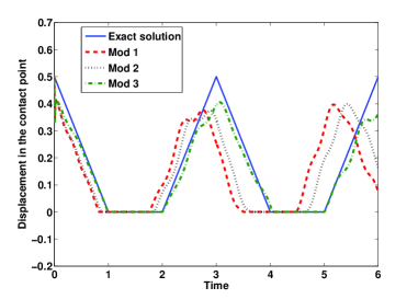
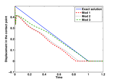
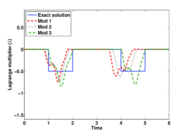
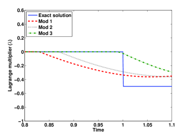
Figure 7: Comparison of analytical $(u,\lambda)$ and approximate $(U^{n}_{h},\lambda^{n})$ solutions for some modified mass matrices in the contact node with Paoli-Schatzman method ($\Delta x=\frac{1}{6}$ and $\Delta t=\frac{1}{100}$).

The time discretization is introduced in this section. To this aim, we divide the time interval $[0,T]$ by $n+1$ discrete time-points such that $0=t_{0}<t_{1}<\ldots<t_{n}=T$. Let $U_{h}^{n}$, $\dot{U}_{h}^{n}$, $\ddot{U}_{h}^{n}$ and $\lambda^{n}$ be the approximations of the displacement $U_{h}(t_{n})$, the velocity $\dot{U}_{h}(t_{n})$, the acceleration $\ddot{U}_{h}(t_{n})$ and the Lagrange multiplier $\lambda(t_{n})$, respectively. We deal with some approximate solutions to Problem (2.1)–(2.3) obtained by using several time-stepping methods like the Newmark, backward Euler and Paoli-Schatzman methods. For each of these time-stepping methods, approximate solutions $(U_{h}^{n},\lambda^{n})$ are exhibited for several mass redistributions and they are compared to the analytical solution $(u,\lambda)$ introduced in Section 4.1. In the numerical experiments presented below, we distinguish the cases that the mass of the contact node that is not redistributed (Mod 1), or uniformly redistributed on all the other nodes (Mod 2), or redistributed only on the nearest neighbor (Mod 3), according to the classification given in the previous section. We show that the efficiency of the mass redistribution method depends on the position of the nodes where the mass is redistributed. Indeed, the numerical experiments highlight that the closer from the contact node the mass is transferred better the approximate solutions are obtained. Then, it is not surprising that the best approximate solution can be expected and indeed it is obtained in the case (Mod 3), where all the mass of the contact node is transferred on the node preceding the contact node, see Figures 3, 5 and 7. Note that the numerical simulations presented below were performed by employing the finite element library Getfem${++}$ (see [ReP]).

4.2.1 The Newmark methods

The Taylor expansions of displacements and velocities neglecting terms of higher order are the underlying concept of the family of Newmark methods, see [New59]. These methods are unconditionally stable for linear elastodynamic problem for $\gamma\geq\tfrac{1}{2}$ and $\beta\geq\tfrac{1}{4}(\tfrac{1}{2}{+}\gamma)^{2}$, see [Hug87, Kre06], but they are also the most popular time-stepping schemes used to solve contact problems. The discrete evolution for the contact problem (2.1)–(2.3) is described by the following finite difference equations:

$$\begin{cases}\text{find }U_{h}^{n+1}:[0,T]\rightarrow\mathbb{R}^{m}\text{ and }\lambda^{n}:[0,T]\rightarrow\mathbb{R}\text{ such that:}\\ U_{h}^{n+1}=U_{h}^{n}+\Delta t\dot{U}_{h}^{n}+\bigl{(}\frac{1}{2}{-}\beta\bigr{)}\Delta t^{2}\ddot{U}_{h}^{n}+\beta\Delta t^{2}\ddot{U}_{h}^{n+1},\\ \dot{U}_{h}^{n+1}=\dot{U}_{h}^{n}+(1{-}\gamma)\Delta t\ddot{U}_{h}^{n}+\gamma\Delta t\ddot{U}_{h}^{n+1},\\ M\ddot{U}_{h}^{n+1}+SU_{h}^{n+1}=-\lambda^{n+1}e_{0}+F^{n+1},\\ 0\leq u_{0}^{n+1}\perp\lambda^{n+1}\leq 0,\end{cases}$$ (4.3)

where $\Delta t$ is a given times step and $(\beta,\gamma)$ are the algorithmic parameters, see [Hug87, Lau03]. Note that $U_{h}^{0}$, $\dot{U}_{h}^{0}$ and $\lambda^{0}$ are given and $\ddot{U}_{h}^{0}$ is evaluated by using the third identity in (4.3). We are particularly interested in the case where $(\beta,\gamma)=(\frac{1}{4},\frac{1}{2})$. This method is called the Crank-Nicolson method, it is second-order consistent and unconditionally stable in the unconstrained case. However the situation is quite different in the case of contact constraints, indeed the order of accuracy is degraded; for further details, the reader is referred to [Hug87, Kre06, GrH07]. The analytical solution $(u,\lambda)$ exhibited in Section 4.1 and the approximate solutions $(U^{n}_{h},\lambda^{n})$ obtained for different mass redistributions are represented on Figure 3. The approximate solution obtained for the nearest neighbor redistribution (Mod 3 on Figure 3) gives much better accuracy than the mass redistribution on all the nodes preceding the contact node (see Mod 2 on Figure 3) and no mass redistribution. This highlighted that the choice for the mass redistribution plays a crucial role.

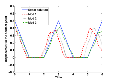
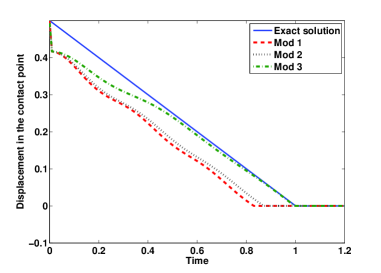
Figure 3: Comparison of analytical $(u,\lambda)$ and approximate $(U^{n}_{h},\lambda^{n})$ solutions for some modified mass matrices in the contact node with Crank-Nicolson method ($\Delta x=\frac{1}{6}$ and $\Delta t=\frac{1}{100}$).

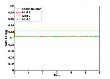
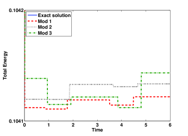
Figure 4: Comparison of the energy associated with analytical solution and the energy associated with approximate solutions for some modified mass matrices with Crank-Nicolson method ($\Delta x=\frac{1}{6}$ and $\Delta t=\frac{1}{100}$). The figure on the right hand side represents a zoom of the figure on the left hand side.

4.2.2 The backward Euler method

We are concerned here with backward Euler’s method which for the contact problem (2.1)–(2.3) is described by the following finite difference equations:

$$\begin{cases}\text{find }U_{h}^{n+1}:[0,T]\rightarrow\mathbb{R}^{m}\text{ and }\lambda^{n}:[0,T]\rightarrow\mathbb{R}\text{ such that:}\\ U_{h}^{n+1}=U_{h}^{n}+\Delta t\dot{U}_{h}^{n+1},\\ \dot{U}_{h}^{n+1}=\dot{U}_{h}^{n}+\Delta t\ddot{U}_{h}^{n+1},\\ M\ddot{U}_{h}^{n+1}+SU_{h}^{n+1}=-\lambda^{n+1}e_{0}+F^{n+1},\\ 0\leq u_{0}^{n+1}\perp\lambda^{n+1}\leq 0.\end{cases}$$ (4.4)

Note that $U_{h}^{0}$, $\dot{U}_{h}^{0}$ and $\lambda^{0}$ are given and $\ddot{U}_{h}^{0}$ is evaluated by using the third equality in (4.4).

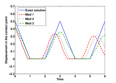
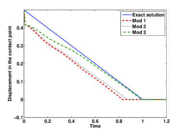
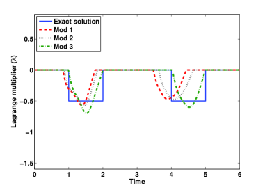
Figure 5: Comparison of analytical $(u,\lambda)$ and approximate $(U^{n}_{h},\lambda^{n})$ solutions for some modified mass matrices in the contact node with backward Euler method ($\Delta x=\frac{1}{6}$ and $\Delta t=\frac{1}{100}$).

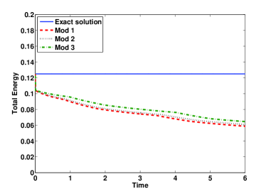
Figure 6: Comparison of energy associated with analytical solution and energy associated with approximate solutions for modified mass matrices with backward Euler method ($\Delta x=\frac{1}{6}$ and $\Delta t=\frac{1}{100}$).

4.2.3 The Paoli-Schatzman methods

We focus on the so-called Paoli–Schatzman method that consists to fix the contact constraint at an intermediate time step. Indeed the method proposed below is a slight modification of Paoli-Schatzman method (see [Pao01, PaS02]) which takes into account the kernel of the modified mass matrix. A simple application of Paoli-Schatzman method based on Newmark scheme to our problem with $\gamma=\frac{1}{2}$ leads to

$$\begin{cases}\text{find }U_{h}^{n+1}:[0,T]\rightarrow\mathbb{R}^{m}\text{ and }\lambda^{n}:[0,T]\rightarrow\mathbb{R}\text{ such that:}\\ \displaystyle{\frac{M(U_{h}^{n+1}{-}2U_{h}^{n}{+}U_{h}^{n-1})}{\Delta t^{2}}+S(\beta U_{h}^{n+1}{+}(1{-}2\beta)U_{h}^{n}{+}\beta U_{h}^{n-1})=-\lambda^{n}e_{0}\textrm{ for all }n\geq 2,}\\ \displaystyle{0\leq u_{0}^{n,e}=}\frac{u_{0}^{n+1}+eu_{0}^{n-1}}{1+e}\perp\lambda^{n}\leq 0,\\ U_{0}\text{ and }U_{1}\text{ given}.\end{cases}$$ (4.5)

Here $e$ belongs to $[0,1]$ and is aimed to be interpreted as a restitution coefficient. Note that $U_{h}^{0}$ and $U_{h}^{1}$ are given data and $U_{h}^{1}$ can be evaluated by a one step scheme. We may observe that taking $M=M^{\text{mod}}$ in (4.5), we are not able to resolve the problem on the kernel of $M^{\text{mod}}$. That is the reason why, $SU_{h}^{n-1}$ as well as $SU_{h}^{n}$ are projected on the orthogonal of the kernel of $M$. We are interested here in Paoli-Schatzman’s method with $(\beta,e)=(\frac{1}{4},1)$. Note that the stability result immediately follows from [DuP06].

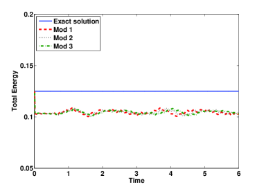
Figure 8: Comparison of energy associated with analytical solution and energy associated with approximate solutions for some modified mass matrices with Paoli-Schatzman method ($\Delta x=\frac{1}{6}$ and $\Delta t=\frac{1}{100}$).

5 A hybrid time integration scheme

Generally, the second order schemes illustrate one of the difficulties when solving contact problems, namely some oscillations for energy associated with approximate solutions obtained for different choices of mass redistribution can be observed after each impact takes place, for instance see Figure 4. To overcome this problem, a hybrid time integration scheme is introduced in this section. More precisely, the scheme $(\mathrm{P}_{U_{h}}^{\textrm{mod}})$ is modified to be an unconditionally stable and a second order in time scheme; the linear part of $(\mathrm{P}_{U_{h}}^{\textrm{mod}})$ is discretized by using the midpoint method while the non-linear part is discretized by using the Crank-Nicolson as well as the midpoint methods. Observe that the midpoint method for the linear problem is energy conserving. The proposed hybrid time integration scheme inspired from [CHR14] reads as follows:

$$(\mathrm{P}_{U_{h}}^{\textrm{hyb}})\hskip 20.00003pt\begin{cases}\text{Find }U_{h}:[0,T]\rightarrow\mathbb{R}^{m-1}\text{ such that}\\ {U}_{h}^{n+1}={U}_{h}^{n}+\frac{\Delta t}{2}\big{(}{\dot{U}}_{h}^{n+1}+{\dot{U}}_{h}^{n}\big{)}\\ {\dot{U}}_{h}^{n+1}={\dot{U}}_{h}^{n}+\frac{\Delta t}{2}\big{(}{\ddot{U}}_{h}^{n+1}+{\ddot{U}}_{h}^{n}\big{)}\\ {M^{*}}{\ddot{U}}_{h}^{n+\frac{1}{2}}+{S^{*}}{U}_{h}^{n+\frac{1}{2}}=F+\frac{H(-u_{1}^{n})}{2h}(u_{1}^{n}+u_{1}^{n+1})^{+}{e}_{1}+\frac{H(u_{1}^{n})}{2h}((u_{1}^{n})^{+}+(u_{1}^{n+1})^{+}){e}_{1},\end{cases}$$

where $V^{n+\frac{1}{2}}\overset{\text{\tiny\rm def}}{=}\frac{V^{n+1}+V^{n}}{2}$ and $H$ is defined by

$$H(s)\overset{\text{\tiny\rm def}}{=}\begin{cases}1\text{ if }s>0,\\ \tfrac{1}{2}\text{ if }s=0,\\ 0\text{ otherwise}.\end{cases}$$

We assume that the density of external forces $F$ does not depend on time. Observe that $\frac{1}{2h}((u_{1}^{n})^{+}+(u_{1}^{n+1})^{+}){e}_{1}$ and $\frac{1}{2h}(u_{1}^{n}+u_{1}^{n+1})^{+}{e}_{1}$ correspond to the contribution of Crank-Nicolson and midpoint methods, respectively.

The discrete evolution of the total energy is preserved in the purely elastic case when the density of external forces vanishes, see [Lau03]. However, the situation quite different in the case of contact constraints, the order of accuracy is degraded and , for further details see [Hug87, Kre06, GrH07]. Let us define now the energy evolution by $\Delta\mathcal{E}_{h}^{n}\overset{\text{\tiny\rm def}}{=}\mathcal{E}_{h}^{n+1}-\mathcal{E}_{h}^{n}$, where $\mathcal{E}_{h}^{n}$ is assumed to be given by an algorithmic approximation of the energy $\mathcal{E}_{h}(t_{n})$ defined in (3.4). We evaluate now $\Delta\mathcal{E}_{h}^{n}$ by using the midpoint scheme. More precisely, we get

$$\Delta\mathcal{E}_{h}^{n}=({\dot{U}}_{h}^{n+\frac{1}{2}})^{\mathsf{T}}{M^{*}}(\Delta t{\ddot{U}}_{h}^{n+\frac{1}{2}})+({U}_{h}^{n+\frac{1}{2}})^{\mathsf{T}}{S^{*}}(\Delta t{\dot{U}}_{h}^{n+\frac{1}{2}})-(\Delta t{\dot{U}}_{h}^{n+\frac{1}{2}})^{\mathsf{T}}F+\tfrac{((u_{1}^{n})^{+})^{2}-((u_{1}^{n+1})^{+})^{2}}{2h}.$$

Since ${M^{*}}$ is symmetric matrix, it comes that

$$\Delta\mathcal{E}_{h}^{n}={\Delta t}({\dot{U}}^{n+\tfrac{1}{2}})^{\mathsf{T}}\bigl{(}\tfrac{H(-u_{1}^{n})}{2h}(u_{1}^{n}+u_{1}^{n+1})^{+}{e}_{1}+\tfrac{H(u_{1}^{n})}{2h}((u_{1}^{n})^{+}+(u_{1}^{n+1})^{+}){e}_{1}\bigr{)}+\tfrac{((u_{1}^{n})^{+})^{2}-((u_{1}^{n+1})^{+})^{2}}{2h},$$

which implies that

$$\Delta\mathcal{E}_{h}^{n}=(u_{1}^{n+1}{-}u_{1}^{n})\bigl{(}\tfrac{H(-u_{1}^{n})}{2h}(u_{1}^{n}+u_{1}^{n+1})^{+}{e}_{1}+\tfrac{H(u_{1}^{n})}{2h}((u_{1}^{n})^{+}+(u_{1}^{n+1})^{+}){e}_{1}\bigr{)}+\tfrac{((u_{1}^{n})^{+})^{2}-((u_{1}^{n+1})^{+})^{2}}{2h}.$$

We establish below that the energy evolution by $\Delta\mathcal{E}_{h}^{n}$ is nonpositive, namely the energy associated with the hybrid scheme decreases in time. This result is summarized in the following lemma:

Lemma 5.1.

Assume that the density of external forces $F$ does not depend on time. Then the energy evolution $\Delta\mathcal{E}_{h}^{n}$ is nonpositive for all $n>0$.

Proof.

We distinguish five cases depending on the values taken by $u^{n}_{1}$ and $u^{n+1}_{1}$. More precisely, we get

1. If $u^{n}_{1}<0$ and $u^{n+1}_{1}\leq 0$ then

   $$\Delta\mathcal{E}_{h}^{n}=\tfrac{1}{2h}(u_{1}^{n+1}-u_{1}^{n})(u_{1}^{n}+u_{1}^{n+1})^{+}-\tfrac{1}{2h}((u_{1}^{n+1})^{+})^{2}=0.$$

2. If $u^{n}_{1}<0$ and $u^{n+1}_{1}>0$ then

   $$\Delta\mathcal{E}_{h}^{n}=\tfrac{1}{2h}(u_{1}^{n+1}-u_{1}^{n})(u_{1}^{n}+u_{1}^{n+1})^{+}-\tfrac{1}{2h}((u_{1}^{n+1})^{+})^{2}<0.$$

3. If $u^{n}_{1}>0$ and $u^{n+1}_{1}\leq 0$ then

   $$\Delta\mathcal{E}_{h}^{n}=\tfrac{1}{2h}(u_{1}^{n+1}-u_{1}^{n})(u_{1}^{n})^{+}+\tfrac{1}{2h}((u_{1}^{n})^{+})^{2}<0.$$

4. If $u^{n}_{1}>0$ and $u^{n+1}_{1}>0$ then

   $$\Delta\mathcal{E}_{h}^{n}=\tfrac{1}{2h}(u_{1}^{n+1}-u_{1}^{n})((u_{1}^{n+1})^{+}+(u_{1}^{n})^{+})-\tfrac{1}{2h}((u_{1}^{n+1})^{+})^{2}+\tfrac{1}{2h}((u_{1}^{n})^{+})^{2}=0.$$

5. If $u^{n}_{1}=0$ then

   $$\Delta\mathcal{E}_{h}^{n}=\tfrac{1}{2h}(u_{1}^{n+1})(u_{1}^{n+1})^{+}-\tfrac{1}{2h}((u_{1}^{n+1})^{+})^{2}=0.$$

This proves the lemma. ∎

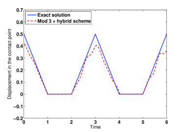
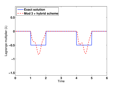
Figure 9: Comparison of analytical $(u,\lambda)$ and approximate $(U^{n}_{h},\lambda^{n})$ solutions for the modified mass matrix (Mod 3), in the contact node with hybrid scheme ($\Delta x=\frac{1}{6}$ and $\Delta t=\frac{1}{100}$).

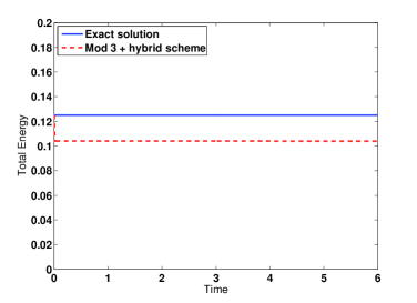
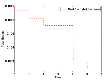
Figure 10: Comparison of the energy associated with analytical solution and the energy associated with approximate solutions for the modified mass matrix (Mod 3) with hybrid scheme ($\Delta x=\frac{1}{6}$ and $\Delta t=\frac{1}{100}$). The figure on the right hand side represents a zoom of the figure on the left hand side.

The numerical experiments presented on Figures 9 and 10 are obtained by using a new hybrid scheme where the mass of the contact node is redistributed on the node preceding the contact. This scheme circumvents the undesirable oscillations at the contact boundary and it prevents as well the small oscillations of the evolution of total energy occurring for Newmark methods (see Figures 4 and 8). Finally, the energy evolution $\Delta\mathcal{E}_{h}^{n}$ is nonpositive for all $n>0$ and it is much smaller than the energy evolution obtained by using implicit Euler method (compare with Figure 6).

6 Conclusion

This manuscript focuses on the weighted mass redistribution method which is particularly well adapted to approximate elastodynamic contact problems. This method leads to well-posed and energy conserving semi-discretization of elastodynamic contact problems. Furthermore, it prevents some undesirable oscillations at the contact boundary as well as some phase shift between approximate and analytical solutions. The efficiency of the weighted mass redistribution method depends on the position of the nodes where the mass is redistributed; the closer the mass of the contact node is transferred, the better are the approximate solutions. These results seem also valid in higher space dimensions, and in particular in 2D space (see Table 1). Indeed the weight mass redistribution on the nodes before the contact (Mod 3) gives much better absolute error than in the cases where any redistribution is done (Mod 1) or where the mass is just eliminated from the contact nodes (Mod 2). The total error rates are evaluated for the space steps $\Delta x_{1}=\Delta x_{2}=0.05$. However the energy associated with the Newmark and Paoli-Schatzman methods in time have small oscillations, (see for instance Figure 4), which is unacceptable from a mechanical view point. Then a new hybrid scheme having the properties to be an unconditionally stable has been developed giving some promising numerical results. It allow to have a far better approximation compared to existing unconditionally stable scheme on the implicit Euler scheme (compare Figures 6 and 10).

Method employed	Mod 1	Mod 2	Mod 3
${\lVert U_{h}^{n}{-}U\rVert_{{{\mathrm{L}}^{\infty}(0,T;{\mathrm{L}}^{2}((0,1)\times(0,1)))}}}$	0.0104	0.0046	0.0038

Table 1: Total error rates for the displacement

Acknowledgments

The support of the GAČR Grant GA15-12227S and RVO: 67985840, and of the AVČR–CNRS Project “Mathematical and numerical analysis of contact problems for materials with memory” is gratefully acknowledged.

References

• [Bre73] H. Brezis. Opérateurs maximaux monotones et semi-groupes de contractions dans les espaces de Hilbert. North-Holland Publishing Co., Amsterdam, 1973. North-Holland Mathematics Studies, No. 5. Notas de Matemática (50).
• [Bre83] H. Brezis. Analyse fonctionnelle. Collection Mathématiques Appliquées pour la Maîtrise. [Collection of Applied Mathematics for the Master’s Degree]. Masson, Paris, 1983. Théorie et applications. [Theory and applications].
• [CTK91] N. J. Carpenter, R. L. Taylor, and M. G. Katona. Lagrange constraints for transient finite element surface contact. Int. J. Numer. Meth. Engng., 32:103–128, 1991.
• [ChL98] V. Chawla and T. A. Laursen. Energy consistent algorithms for frictional contact problems. Internat. J. Numer. Methods Engrg., 42(5):799–827, 1998.
• [CHR14] F. Chouly, P. Hild, and Y. Renard. A Nitsche finite element method for dynamic contact: 1. space semi-discretization and time-marching schemes. 2. stability of the schemes and numerical experiments. ESAIM: Math. Model. Numer. Anal., 2014.
• [CrM84] M. Crouzeix and A. L. Mignot. Analyse numérique des équations différentielles. Collection Mathématiques Appliquées pour la Maîtrise, Masson, Paris, 1984.
• [DP*12] F. Dabaghi, A. Petrov, J. Pousin, and Y. Renard. Convergence of mass redistribution method for the wave equation with a unilateral constraint at the boundary. ESAIM: Math. Model. Numer. Anal., 48:1147–1169, 2014.
• [DP*13] F. Dabaghi, A. Petrov, J. Pousin, and Y. Renard. Numerical approximations of a one dimensional elastodynamic contact problem based on mass redistribution method. Submitted, 2013.
• [DKE08] P. Deuflhard, R. Krause, and S. Ertel. A contact-stabilized Newmark method for dynamical contact problems. Internat. J. Numer. Methods Engrg., 73(9):1274–1290, 2008.
• [DEP11] D. Doyen, A. Ern, and S. Piperno. Time-integration schemes for the finite element dynamic Signorini problem. SIAM J. Sci. Comput., 33(1):223–249, 2011.
• [DuP06] Y. Dumont and L. Paoli. Vibrations of a beam between obstacles. Convergence of fully discretized approximation. ESAIM Math. Model. Numer. Anal., 40(4):705–734, 2006.
• [Fuc76] S. Fučík. Boundary value problems with jumping nonlinearity. Časopis Pěst. Mat., 1:69–87, 1976.
• [GrH07] E. Grosu and I. Harari. Stability of semidiscrete formulations for elastodynamics at small time steps. Finite Elem. Anal. Des., 43(6-7):533–542, 2007.
• [Hug87] T. J. R. Hughes. The finite element method. Prentice Hall Inc., Englewood Cliffs, NJ, 1987. Linear static and dynamic finite element analysis. With the collaboration of Robert M. Ferencz and Arthur M. Raefsky.
• [Kim89] J. U. Kim. A boundary thin obstacle problem for a wave equation. Comm. Partial Differential Equations, 14(8–9):1011–1026, 1989.
• [Kre06] S. Krenk. Energy conservation in Newmark based time integration algorithms. Comput. Methods Appl. Mech. Engrg., 195(44–47):6110–6124, 2006.
• [KLR08] H. B. Khenous, P. Laborde, and Y. Renard. Mass redistribution method for finite element contact problems in elastodynamics. Eur. J. Mech. A Solids, 27(5):918–932, 2008.
• [HHW08] C. Hager, S. Hüeber, and B. I. Wohlmuth. A stable energy-conserving approach for frictional contact problems based on quadrature formulas. Internat. J. Numer. Methods Engrg., 73(2):205–225, 2008.
• [Hau10] P. Hauret. Mixed interpretation and extensions of the equivalent mass matrix approach for elastodynamics with contact. Comput. Methods Appl. Mech. Engrg., 199(45-48):2941–2957, 2010.
• [Hug03] T. J. R. Hughes. The finite element method. Linear static and dynamic finite element analysis. Prentice-Hall, Engewood, 2003.
• [LaC97] T. A. Laursen and V. Chawla. Design of energy conserving algorithms for frictionless dynamic contact problems. Internat. J. Numer. Methods Engrg., 40(5):863–886, 1997.
• [LaL02] T. A. Laursen and G. R. Love. Improved implicit integrators for transient impact problems–geometric admissibility within the conserving framework. Internat. J. Numer. Methods Engrg., 53(2):245–274, 2002.
• [Lau03] T. A. Laursen. Computational contact and impact mechanics. Fundamentals of modeling interfacial phenomena in nonlinear finite element analysis. Springer-Verlag, Berlin Heidelberg New York, 2003.
• [LeS84] G. Lebeau and M. Schatzman. A wave problem in a half-space with a unilateral constraint at the boundary. J. Differential Equations, 53(3):309–361, 1984.
• [LiR11] T. Ligurský and Y. Renard. A well-posed semi-discretization of elastodynamic contact problems with friction. Quart. J. Mech. Appl. Math., 64(2):215–238, 2011.
• [New59] N. Newmark. A method of computational for structural dynamics. ASCE, J. Eng. Mech. Div., Vol. 85 No. EM3, 1959.
• [Pao01] L. Paoli. Time discretization of vibro-impact. Philos. Trans. Roy. Soc. London Ser. A, 359(1789):2405–2428, 2001. Non-smooth mechanics.
• [PaS93] L. Paoli and M. Schatzman. Schéma numérique pour un modèle de vibrations avec contraintes unilatérales et perte d’énergie aux impacts, en dimension finie. C. R. Acad. Sci. Paris Sér. I Math., 317(2):211–215, 1993.
• [PaS99] L. Paoli and M. Schatzman. Approximation et existence en vibro-impact. C. R. Acad. Sci. Paris Sér. I Math., 329(12):1103–1107, 1999.
• [PaS02] L. Paoli and M. Schatzman. A numerical scheme for impact problems, I and II. SIAM J. Numer. Anal., 40:702–733; 734–768, 2002.
• [ReP] Y. Renard and J. Pommier. Getfem++. An Open Source generic C++ library for finite element methods, http://home.gna.org/getfem.
• [Ren10] Y. Renard. The singular dynamic method for constrained second order hyperbolic equations: application to dynamic contact problems. J. Comput. Appl. Math., 234(3):906–923, 2010.
• [Sch80] M. Schatzman. A hyperbolic problem of second order with unilateral constraints: the vibrating string with a concave obstacle. J. Math. Anal. Appl., 73(1):138–191, 1980.
• [ScB89] M. Schatzman and M. Bercovier. Numerical approximation of a wave equation with unilateral constraints. Math. Comp., 53:55–79,1989.