Linear minimum mean square filters for Markov jump linear systems

Abstract

New linear minimum mean square estimators are introduced in this paper by considering a cluster information structure in the filter design. The set of filters constructed in this way can be ordered in a lattice according to the refines of clusters of the Markov chain, including the linear Markovian estimator at one end (with only one cluster) and the Kalman filter at the other hand (with as many clusters as Markov states). The higher is the number of clusters, the heavier are pre-compuations and smaller is the estimation error, so that the cluster cardinality allows for a trade-off between performance and computational burden. In this paper we propose the estimator, give the formulas for pre-computation of gains, present some properties, and give an illustrative numerical example.

1 Introduction

There is a vast number of applications benefiting from the nice properties of the Kalman filter (KF). Among these properties, the possibility of pre-computation of gains [1, 7] is of much relevance for applications. However, in some cases pre-computation is not possible or viable due to missing a priori relevant information. This is the case when using the KF to estimate the state of Markov jump linear systems (MJLS), since the parameters are not known prior to the current time instant $k$, in fact they depend on the Markov chain current state $\theta(k)$. Then, to use KF for MJLS one needs to do either online computation of the gains or offline pre-computation of a number of sample path dependent gains, a figure that grows exponentially with time.

This drawback of KF for MJLS is one of the main motivations behind the emergence of other filters for this class of systems, see e.g. [2, 4, 5, 6]. Among them, the one that is closer to the KF in terms of structure and performance is the linear minimum mean square estimator (LMMSE) first introduced for MJLS in [3]. Indeed, as we shall see later, the LMMSE computation relies on coupled Riccati equations that are quite similar to the ones arising in Kalman filtering. Another similarity is that both are optimal in the mean square error sense, although under different constraints. The main dissimilarity with KF lies in the fact that, instead of having path dependent gains, the LMMSE has sets of $N$ gains, $N$ being the cardinality of the Markov state space (which we assume finite in this paper), that are precomputed based on the system matrices and the initial distribution of $\theta$. During application, after observing $\theta(k)$ one picks the corresponding gain from the precomputed sets of gains. In this way, one obtains the best estimate for the system state $x_{k}$ among all estimators that are linear and Markovian, these being precisely the constraints we mentioned before.

However, there is currently no intermediary solution between the KF and the LMMSE in literature. In this paper we provide a “lattice” of filters bridging the KF to the LMMSE by relaxing the markovianity constraint and allowing clustered information of the Markov chain to be considered when designing the filter gains. By clustered information, we mean that we have a partition of the state space of the Markov chain into several classes called clusters, and we observe the trajectory of classes the chain belongs to along time. The clusters may be chosen as they are considered as a design parameter, establishing a trade-off between complexity and performance that can be explored in practical systems aiming at the best feasible performance. At one extreme when only one cluster is taken into account our filter is equivalent to the LMMSE, and at another extreme with $N$ clusters we retrieve the Kalman filter; intermediary number of clusters leads to filters with variable performances and computational burden. Reasonably enough, the higher is the number of clusters the smaller is the attained estimation error and higher is the number of gains to compute.

We start with a simple, precise formulation of the optimal estimation problem in Section 2, with the estimator in the classical form of Luenberger observers. We then proceed in Section 3 to a constructive proof that evaluates the estimation error and uses the completion of squares method to obtain the optimal gains. Some remarks on how the proposed class of estimators includes both the KF and LMMSE, and on the number of gains and Riccati-like equations to be precomputed, are presented. Some variants of the studied optimization problem and how to extend optimality to general estimators are briefly discussed in Section 4. We have also included a numerical example in Section 5 comparing the computational burden in terms of CPU time and the estimation error computed both via Monte Carlo simulation and via the proposed formula. The example makes clear that the performance is strongly dependent on the number of clusters and how the Markov states are distributed in the clusters.

2 Problem formulation

Consider the MJLS

$$x_{k+1} =A_{\theta(k)}x_{k}+G_{\theta(k)}w_{k}$$ (1)

$$y_{k} =L_{\theta(k)}x_{k}+H_{\theta(k)}w_{k},\qquad k\geq 0,$$

with initial condition $x_{0}\sim N(\bar{x},\Psi)$ where $N(\bar{x},\Psi)$ is the normal distribution with mean $\bar{x}$ and covariance matrix $\Psi$. The variable $\theta(k)$ denotes the state of a Markov chain with finite state space $\{1,2,\ldots,N\}$ and initial distribution $\pi_{0}=[\text{Pr}(\theta(0)=1)\,\cdots\text{Pr}(\theta(0)=N)]$. The noise sequence $w$ is independent from $x_{0}$ and the Markov chain $\theta$, $E[w_{k}]=0$ and $E[w_{k}w_{k}^{\prime}]$ is the identity matrix for all $k$. We assume that $G_{i}H_{i}^{\prime}=0$ and $H_{i}H_{i}^{\prime}>0$, $1\leq i\leq N$. We shall consider Luenberger observers in the form

$$\widehat{x}_{k+1} =A_{\theta(k)}\widehat{x}_{k}+M_{k}(y_{k}-L_{\theta(k)}\widehat{x}_{k}),$$ (2)

where matrix $M_{k}$ is referred to as the filter gain, and the initial estimate is given by $\widehat{x}_{0}=\bar{x}$. This produces an estimation error $\widetilde{x}=x-\widehat{x}$ satisfying

$$\widetilde{x}_{k+1} =(A_{\theta(k)}-M_{k}L_{\theta(k)})\widetilde{x}_{k}+(G_{\theta(k)}-M_{k}H_{\theta(k)})w_{k},$$ (3)

and $\widetilde{x}_{0}=x_{0}-\bar{x}\sim N(0,\Psi)$.

As for the Markov chain, we consider a partition $S_{1},\ldots,S_{N_{C}}$ for its state space, and employ the variable $\rho(k)$ to indicate the partition being visited at time $k$, that is,

$$\rho(k)=\sum_{m=1}^{N_{C}}m\times\mathbbm{1}_{\{\theta(k)\in S_{m}\}}.$$

We assume that the observations of $\rho$ up to time $k$ are available to calculate the filter gains. We also assume that the jump variable $\theta$ at time $k$ is available, however in the clustered information filter we do not take into account its past values, that is, $\theta(0),\ldots,\theta(k-1)$ are not taken into account when calculating the gain (to avoid an excessive number of branches, as explained earlier). Moreover, the gain should not depend on future information, as it has to be implemented at every time instant $k$. Therefore, we impose that the filter matrices at time instant $k$ are in the form

$$M_{k} =h_{k}(\rho(0),\ldots,\rho(k-1),\theta(k)),\quad k\geq 0$$ (4)

for measurable functions $h_{k}$. Gains satisfying this constraint are referred to as feasible gains. We are interested in obtaining the minimum mean square state estimation at a given time $s\geq 0$, leading to the optimization problem

$$\min_{M_{0},\ldots,M_{s}}E\{\|x_{s}-\widehat{x}_{s}\|^{2}|\mathcal{R}_{s}\},\qquad\text{s.t.\leavevmode\nobreak\ }\eqref{eq-info-constraint},$$ (5)

where we write $\mathcal{R}_{s}=\{\rho(0),\ldots,\rho(s),y(0),\ldots,y(s),\theta(s)\}$ for ease of notation. We refer to the filter (3) satisfying (5) as the clustered information LMMSE, or CLMMSE for short.

3 Clustered information LMMSE computation

Consider the MJLS in (1) and the filter in (3) with an arbitrary sequence of feasible gains $M=\{M_{k},k\geq 0\}.$ For each $k\geq 0$, $0\leq i\leq N$ and $0\leq\ell_{m}\leq M$, $0\leq m\leq k-1$, we define

$$X_{\ell_{0},\ldots,\ell_{k-1},i,k}(M)=E(\widetilde{x}_{k}\widetilde{x}_{k}^{\prime}\mathbbm{1}_{\{\rho(0)=\ell_{0},\ldots,\rho(k-1)=\ell_{k-1},\theta(k)=i\}}).$$ (6)

The variable $X$ plays an important role in the derivation of the formula for the optimal filter because the optimal gains $M^{\star}=\{M_{k}^{\star},0\leq k\leq s\}$ are such that $X_{\ell_{0},\ldots,\ell_{k-1},i,k}(M^{\star})=Y_{\ell_{0},\ldots,\ell_{k-1},i,k}$ where $Y$ is the solution of a Riccati-like equation, as we shall see in the next theorem. The physical interpretation for $X$ is that, when divided by $\text{Pr}(\rho(0)=\ell_{0},\ldots,\rho(k-1)=\ell_{k-1},\theta(k)=i)$ it gives the conditional error covariance matrix, e.g. it coincides with the filtering Riccati equation of the Kalman filter when $N=N_{C}$ (as many clusters as Markov states).

Example 3.1

We illustrate the notation introduced in (6) on a simple example. Consider the MJLS (1) with $A_{i}=G_{i}=1$, $1\leq i\leq 3$, $\Psi=1$, $\bar{x}=0$, the clusters $S_{1}=\{1,2\}$, $S_{2}=\{3\}$, initial distribution $\pi_{0}=[0.5\;0.3\;0.2]$ and probability matrix

$$P=\begin{bmatrix}0.5&0.4&0.1\\ 1&0&0\\ 0.5&0&0.5\end{bmatrix}.$$

Consider trivial gains $M_{k}=0$, so that $\widetilde{x}_{k}=x_{k}$ and $E(\widetilde{x}_{k+1}\widetilde{x}_{k+1}^{\prime})=E(\widetilde{x}_{k}\widetilde{x}_{k}^{\prime})+1$. Moreover, the estimation error and the Markov state are independent because all modes are identical, then $X_{\ell_{0},\ldots,\ell_{k-1},i,k}(M)=E(\widetilde{x}_{k}\widetilde{x}_{k}^{\prime})\text{Pr}(\rho(0)=\ell_{0},\ldots,\rho(k-1)=\ell_{k-1},\theta(k)=i).$ For instance, for $\ell_{0}=1$, $i=2$ and $k=1$ we have

$$X_{1,2,1} =E(\widetilde{x}_{1}\widetilde{x}_{1}^{\prime})\text{Pr}(\rho(0)=1,\theta(1)=2)=2\,\text{Pr}(\theta(1)=2|\rho(0)=1)\text{Pr}(\rho(0)=1)$$

$$=2\,\text{Pr}(\rho(0)=1)\Big{(}\sum_{j\in S_{\ell_{0}}}\text{Pr}(\theta(1)=2|\rho(0)=1,\theta(0)=j)\text{Pr}(\theta(0)=j|\rho(0)=1)\Big{)}$$

$$=2\times 0.8\times(0.4\times(0.5/0.8)+0\times(0.3/0.8))=0.4.$$

Similarly, $X_{1,1,1}=1.1$, $X_{1,3,1}=0.1$, $X_{2,1,1}=0.2$, $X_{2,2,1}=0$ and $X_{2,3,1}=0.2$. Note from (6) that summing $X$ in the indexes corresponding to $\ell$ and $i$ we obtain $E(\widetilde{x}_{k}\widetilde{x}_{k}^{\prime})$, e.g. from the above we have $E(\widetilde{x}_{1}\widetilde{x}_{1}^{\prime})=2$.

Coupled Riccatis of the CLMMSE

the optimal gain sequence can be (pre-)computed based on the following sets of matrices. Let $Y_{i,0}=\pi_{i}(0)\Psi$ for each $1\leq i\leq N$. For each $k\geq 1$, let $0\leq m\leq k-1$ and compute for each $0\leq i\leq N$ and $0\leq\ell_{m}\leq M$,

$$Y_{\ell_{0},\ldots,\ell_{k-1},i,k}=\begin{cases}0,&p_{\ell_{0},\ldots,\ell_{k-1},i,k}=0,\\ \\ \begin{aligned} &\sum_{j\in\widetilde{S}}p_{ji}\big{[}A_{j}Y_{\ell_{0},\ldots,\ell_{k-2},j,k-1}A_{j}^{\prime}+p_{\ell_{0},\ldots,\ell_{k-2},j}G_{j}G_{j}^{\prime}\\ &\quad\qquad+A_{j}Y_{\ell_{0},\ldots,\ell_{k-2},j,k-1}L_{j}^{\prime}\big{(}L_{j}Y_{\ell_{0},\ldots,\ell_{k-2},j,k-1}L_{j}^{\prime}\\ &\quad\qquad+p_{\ell_{0},\ldots,\ell_{k-2},j,k-1}H_{j}H_{j}^{\prime}\big{)}^{-1}L_{j}Y_{\ell_{0},\ldots,\ell_{k-2},j,k-1}A_{j}^{\prime}\big{]},\end{aligned}&\text{otherwise,}\end{cases}$$ (7)

where we denote

$$p_{\ell_{0},\ldots,\ell_{k-1},i,k} =\text{Pr}(\rho(0)=\ell_{0},\ldots,\rho(k-1)=\ell_{k-1},\theta(k)=i),$$

$$\widetilde{S} =\{j\in S_{\ell_{k-1}}:p_{\ell_{0},\ldots,\ell_{k-2},j,k-1}\not=0\}.$$

Theorem 3.2

Given the realization of $\theta(k)$, $k\leq s$, and the corresponding cluster observations $\rho(0),\ldots,\rho(s-1)$, the gains $M^{\star}=\{M^{\star}_{0},\ldots,M^{\star}_{s}\}$ of the LMMSE can be computed for each $k\leq s$ as

$$M^{\star}_{k}=\begin{cases}0,&\text{Pr}(\rho(0),\ldots,\rho(k-1),\theta(k))=0,\\ \begin{aligned} A_{\theta(k)}&Y_{\rho(0),\ldots,\rho(k-1),\theta(k),k}L_{\theta(k)}^{\prime}\big{(}L_{\theta(k)}Y_{\rho(0),\ldots,\rho(k-1),\theta(k),k}L_{\theta(k)}^{\prime}\\ &+\text{Pr}(\rho(0),\ldots,\rho(k-1),\theta(k))H_{\theta(k)}H_{\theta(k)}^{\prime}\big{)}^{-1},\end{aligned}&\text{otherwise,}\end{cases}$$ (8)

where $Y$ is given in (7). Moreover, the conditional second moment of the estimation error is given, for each $k\leq s$, by

$$X_{\rho(0),\ldots,\rho(k-1),\theta(k),k}(M^{\star})=Y_{\rho(0),\ldots,\rho(k-1),\theta(k),k},$$ (9)

and it is optimal in the sense that, for any gain sequence $M=\{M_{0},\ldots,M_{s}\}$,

$$X_{\rho(0),\ldots,\rho(k-1),\theta(k),k}(M^{\star})\leq X_{\rho(0),\ldots,\rho(k-1),\theta(k),k}(M),\quad 0\leq k\leq s.$$ (10)

Proof We start showing that (9) and (10) are true for the gains prescribed in (8). We proceed by induction in $k$. For the time instant $k=0$ we have that the initial estimate is given by $\widehat{x}_{0}=\bar{x}$, yielding $\widetilde{x}_{0}=x_{0}-\bar{x}\sim N(0,\Psi)$ (irrespectively of the filter gains), hence

$$X_{i,0}(M^{\star})=X_{i,0}(M)=E(\widetilde{x}_{0}\widetilde{x}_{0}^{\prime}\mathbbm{1}_{\{\theta(0)=i\}})=E(\widetilde{x}_{0}\widetilde{x}_{0}^{\prime})E(\mathbbm{1}_{\{\theta(0)=i\}})=\Psi\pi_{i}(0)=Y_{i,0}.$$ (11)

By the induction hypothesis we assume that (9) and (10) are valid for some $0\leq k<s$. In order to complete the induction, we now consider the time instant $k+1$. For a filter with an arbitrary sequence of easible gains, denoted by $M=\{M_{0},\ldots,M_{s}\}$, and a given realization $\rho(0)=\ell_{0},\ldots,\rho(k)=\ell_{k},\theta(k+1)=i$ we have

$$X_{\ell_{0},\ldots,\ell_{k},i,k+1}(M)=E(\widetilde{x}_{k+1}\widetilde{x}_{k+1}^{\prime}\mathbbm{1}_{\{\rho(0)=\ell_{0},\ldots,\rho(k)=\ell_{k},\theta(k+1)=i\}}).$$

Note that the above quantity turns out to be zero whenever $p_{\ell_{0},\ldots,\ell_{k},i,k+1}=0$, irrespectively of $M$, which makes (9) and (10) trivially true for $k+1$ in this case. Now, in case $p_{\ell_{0},\ldots,\ell_{k},i,k+1}\not=0$ we write

$$X_{\ell_{0},\ldots,\ell_{k},i,k+1}(M)=E(\widetilde{x}_{k+1}\widetilde{x}_{k+1}^{\prime}\mathbbm{1}_{\{\rho(0)=\ell_{0},\ldots,\rho(k)=\ell_{k},\theta(k+1)=i\}})$$ (12)

$$=E\Big{(}\big{(}(A_{\theta(k)}-M_{k}L_{\theta(k)})\widetilde{x}_{k}+(G_{\theta(k)}-M_{k}H_{\theta(k)})w_{k}\big{)}$$

$$\qquad\times\big{(}(A_{\theta(k)}-M_{k}L_{\theta(k)})\widetilde{x}_{k}+(G_{\theta(k)}-M_{k}H_{\theta(k)})w_{k}\big{)}^{\prime}\mathbbm{1}_{\{\rho(0)=\ell_{0},\ldots,\rho(k)=\ell_{k},\theta(k+1)=i\}}\Big{)}$$

$$=E\Big{(}[(A_{\theta(k)}-M_{k}L_{\theta(k)})\widetilde{x}_{k}\widetilde{x}_{k}^{\prime}(A_{\theta(k)}-M_{k}L_{\theta(k)})^{\prime}$$

$$\qquad+(G_{\theta(k)}-M_{k}H_{\theta(k)})w_{k}w_{k}^{\prime}(G_{\theta(k)}-M_{k}H_{\theta(k)})^{\prime}]\mathbbm{1}_{\{\rho(0)=\ell_{0},\ldots,\rho(k)=\ell_{k},\theta(k+1)=i\}}\Big{)}$$

$$=E\Big{(}\sum_{j=1}^{N}[(A_{\theta(k)}-M_{k}L_{\theta(k)})\widetilde{x}_{k}\widetilde{x}_{k}^{\prime}(A_{\theta(k)}-M_{k}L_{\theta(k)})^{\prime}$$

$$\qquad+(G_{\theta(k)}-M_{k}H_{\theta(k)})w_{k}w_{k}^{\prime}(G_{\theta(k)}-M_{k}H_{\theta(k)})^{\prime}]\mathbbm{1}_{\{\rho(0)=\ell_{0},\ldots,\rho(k)=\ell_{k},\theta(k+1)=i,\theta(k)=j\}}\Big{)}$$

$$=E\Big{(}\sum_{j\in S_{\ell_{k}}}[(A_{j}-M_{k}L_{j})\widetilde{x}_{k}\widetilde{x}_{k}^{\prime}(A_{j}-M_{k}L_{j})^{\prime}$$

$$\qquad+(G_{j}-M_{k}H_{j})w_{k}w_{k}^{\prime}(G_{j}-M_{k}H_{j})^{\prime}]\mathbbm{1}_{\{\rho(0)=\ell_{0},\ldots,\rho(k-1)=\ell_{k-1},\theta(k+1)=i,\theta(k)=j\}}\Big{)}$$

where the last equality comes from the fact that $\text{Pr}(\rho(k)=\ell_{k},\theta(k)=j)=0$ whenever $j$ is not in the cluster $S_{\ell_{k}}$, and $\text{Pr}(\rho(k)=\ell_{k},\theta(k)=j))=\text{Pr}(\theta(k)=j)$ otherwise. Resuming the above calculation and writing $\mathcal{R}=\{\rho(0)=\ell_{0},\ldots,\rho(k-1)=\ell_{k-1},\theta(k+1)=i,\theta(k)=j\}$ for ease of notation, we have:

$$X_{\ell_{0},\ldots,\ell_{k},i,k+1}(M) =\sum_{j\in S_{\ell_{k}}}\text{Pr}(\mathcal{R})\big{[}(A_{j}-M_{k}L_{j})E\big{(}\widetilde{x}_{k}\widetilde{x}_{k}^{\prime}\big{|}\mathcal{R})(A_{j}-M_{k}L_{j})^{\prime}$$ (13)

$$\qquad\qquad+(G_{j}-M_{k}H_{j})E\big{(}w_{k}w_{k}^{\prime}\big{|}\mathcal{R})(G_{j}-M_{k}H_{j})^{\prime}\big{]}.$$

From basic properties of the Markov chain we have that $\rho(\ell)$ and $\theta(k+1)$ are conditionally independent given $\theta(k)$, for any $0\leq\ell\leq k-1$. Moreover, from (1), (3) and (4) it can be shown that $\widetilde{x}_{k}$ and $\theta(k+1)$ are conditionally independent given $\theta(k)$, hence we may eliminate $\theta(k+1)=i$ from the first conditional expectation in (13), leading to

$$X {}_{\ell_{0},\ldots,\ell_{k},i,k+1}(M)=\sum_{j\in S_{\ell_{k}}}\text{Pr}(\theta(k+1)=i|\rho(0)=\ell_{0},\ldots,\rho(k-1)=\ell_{k-1},\theta(k)=j)p_{\ell_{0},\ldots,\ell_{k-1},j,k}$$ (14)

$$\qquad\times\big{[}(A_{j}-M_{k}L_{j})E\big{(}\widetilde{x}_{k}\widetilde{x}_{k}^{\prime}\big{|}\rho(0)=\ell_{0},\ldots,\rho(k-1)=\ell_{k-1},\theta(k)=j)(A_{j}-M_{k}L_{j})^{\prime}$$

$$\qquad+(G_{j}-M_{k}H_{j})I(G_{j}-M_{k}H_{j})^{\prime}\big{]}$$

$$=\sum_{j\in\widetilde{S}}p_{ji}\big{[}(A_{j}-M_{k}L_{j})X_{\ell_{0},\ldots,\ell_{k-1},j,k}(M)(A_{j}-M_{k}L_{j})^{\prime}$$

$$\qquad\qquad+p_{\ell_{0},\ldots,\ell_{k-1},j,k}(G_{j}-M_{k}H_{j})(G_{j}-M_{k}H_{j})^{\prime}\big{]},$$

where we denote $\widetilde{S}=\{j\in S_{\ell_{k}}:p_{\ell_{0},\ldots,\ell_{k-1},j,k}\not=0\}$. We now turn our attention to the optimality of $M$. Consider a feasible gain sequence in the form

$$\bar{M}=\{M_{0}^{\star},\ldots,M_{k-1}^{\star},M_{k}\},$$

where $M_{k}$ is the variable to be determined; since $X_{\ell_{0},\ldots,\ell_{k-1},j,k}(\bar{M})$ is a function of $M_{0}^{\star},\ldots,M_{k-1}^{\star}$ only, we can use the induction hypothesis to write

$$X_{\ell_{0},\ldots,\ell_{k-1},j,k}(\bar{M})=Y_{\ell_{0},\ldots,\ell_{k-1},j,k},$$ (15)

$$X_{\ell_{0},\ldots,\ell_{k-1},j,k}(\bar{M})\leq X_{\ell_{0},\ldots,\ell_{k},j,k}(M).$$ (16)

Eq. (16) allows to write $(A_{j}-M_{k}L_{j})(X_{\ell_{0},\ldots,\ell_{k-1},j,k}(\bar{M})-X_{\ell_{0},\ldots,\ell_{k-1},j,k}(M))(A_{j}-M_{k}L_{j})^{\prime}\leq 0$, irrespectively of $M_{k}$, and using (14) we evaluate

$$X_{\ell_{0},\ldots,\ell_{k},i,k+1}(\bar{M})-X_{\ell_{0},\ldots,\ell_{k},i,k+1}(M)$$ (17)

$$=\sum_{j\in\widetilde{S}}p_{ji}\big{[}(A_{j}-M_{k}L_{j})(X_{\ell_{0},\ldots,\ell_{k-1},j,k}(\bar{M})-X_{\ell_{0},\ldots,\ell_{k-1},j,k}(M))(A_{j}-M_{k}L_{j})^{\prime}\leq 0$$

Also, by plugging (15) into (14),

$$X_{\ell_{0},\ldots,\ell_{k},i,k+1} (\bar{M})=\sum_{j\in\widetilde{S}}p_{ji}\big{[}(A_{j}-M_{k}L_{j})Y_{\ell_{0},\ldots,\ell_{k-1},j,k}(\bar{M})(A_{j}-M_{k}L_{j})^{\prime}$$ (18)

$$\qquad+p_{\ell_{0},\ldots,\ell_{k-1},j,k}(G_{j}-M_{k}H_{j})I(G_{j}-M_{k}H_{j})^{\prime}\big{]},$$

and, by completing squares and denoting $\Phi=L_{j}Y_{\ell_{0},\ldots,\ell_{k-1},j,k}L_{j}^{\prime}+\text{Pr}(\rho(0)=\ell_{0},\ldots,\rho(k-1)=\ell_{k-1},\theta(k)=j)H_{j}H_{j}^{\prime}$ for brevity, we obtain

$$X_{\ell_{0},\ldots,\ell_{k},i,k+1}(\bar{M})=\sum_{j\in\widetilde{S}}p_{ji}\big{[}A_{j}Y_{\ell_{0},\ldots,\ell_{k-1},j,k}A_{j}^{\prime}+p_{\ell_{0},\ldots,\ell_{k-1},j,k}G_{j}G_{j}^{\prime}$$ (19)

$$\qquad\qquad\qquad\qquad+\big{(}M_{k}-A_{j}Y_{\ell_{0},\ldots,\ell_{k-1},j,k}L_{j}^{\prime}\Phi^{-1}\big{)}\Phi\big{(}M_{k}-A_{j}Y_{\ell_{0},\ldots,\ell_{k-1},i,k}L_{j}^{\prime}\Phi^{-1}\big{)}^{\prime}$$

$$\qquad\qquad\qquad\qquad-A_{j}Y_{\ell_{0},\ldots,\ell_{k-1},j,k}L_{j}^{\prime}\Phi^{-1}L_{j}Y_{\ell_{0},\ldots,\ell_{k-1},j,k}A_{j}^{\prime}\big{]},$$

thus making clear that the minimal $X$ is attained by setting

$$M_{k} =M_{k}^{\star}=g(\ell_{0},\ldots,\ell_{k-1},j)=A_{j}Y_{\ell_{0},\ldots,\ell_{k-1},i,k}L_{j}^{\prime}\Phi^{-1}$$

$$=A_{j}Y_{\ell_{0},\ldots,\ell_{k-1},i,k}L_{j}^{\prime}\big{(}L_{j}Y_{\ell_{0},\ldots,\ell_{k-1},j,k}L_{i}^{\prime}+p_{\ell_{0},\ldots,\ell_{k-1},j,k}H_{j}H_{j}^{\prime}\big{)}^{-1},$$

whenever $p_{\ell_{0},\ldots,\ell_{k-1},j,k}\not=0$, confirming the second equation in (8); the inverse always exists because we have assumed $H_{i}H_{i}^{\prime}>0$. If $j$ is such that $p_{\ell_{0},\ldots,\ell_{k-1},j,k}=0$ then the gain $M_{k}$ is immaterial for the error covariance, indeed we see from (18) that such gain is not accounted for, so that one can pick $M_{k}=0$, confirming the first equation in (8). Chosing the gain as above we get the gain sequence $M^{\star}=\{M^{\star}_{0},\ldots,M^{\star}_{k}\}$ and

$$X_{\ell_{0},\ldots,\ell_{k},j,k+1}(M^{\star})\leq X_{\ell_{0},\ldots,\ell_{k},j,k+1}(\bar{M}),$$

so that (16) produces

$$X_{\ell_{0},\ldots,\ell_{k},j,k+1}(M^{\star})\leq X_{\ell_{0},\ldots,\ell_{k},j,k+1}(M),$$

which confirms (10) for the time instant $k+1$. Substituting $M_{k}=M_{k}^{\star}$ in (19) we get after some manipulations

$$X_{\ell_{0},\ldots,\ell_{k},i,k+1}(M^{\star}) =\sum_{j\in\widetilde{S}}p_{ji}\big{[}A_{j}Y_{\ell_{0},\ldots,\ell_{k-1},j,k}A_{j}^{\prime}+p_{\ell_{0},\ldots,\ell_{k-1},j,k}G_{j}G_{j}^{\prime}$$

$$\quad\qquad+A_{j}Y_{\ell_{0},\ldots,\ell_{k-1},j,k}L_{j}^{\prime}\big{(}L_{j}Y_{\ell_{0},\ldots,\ell_{k-1},i,k}L_{j}^{\prime}$$

$$\quad\qquad+p_{\ell_{0},\ldots,\ell_{k-1},j,k}H_{j}H_{j}^{\prime}\big{)}L_{j}Y_{\ell_{0},\ldots,\ell_{k-1},j,k}A_{j}^{\prime}\big{]}=Y_{\ell_{0},\ldots,\ell_{k},i,k+1},$$

which confirms (9) for $k+1$, thus completing the induction. It remains only to show the optimality of $M^{\star}$ in terms of (5). This follows directly from (10), in fact,

$$E\{(\widetilde{x}_{k}^{\star})^{\prime}\widetilde{x}_{k}^{\star}\} =\sum E((\widetilde{x}_{k}^{\star})^{\prime}\widetilde{x}_{k}^{\star}\mathbbm{1}_{\{\rho(0)=\ell_{0},\ldots,\rho(k-1)=\ell_{k-1},\theta(k)=i\}})$$

$$=\sum\text{tr}(X_{\ell_{0},\ldots,\ell_{k-1},i,k}(M^{\star}))$$

$$\leq\sum\text{tr}(X_{\ell_{0},\ldots,\ell_{k-1},i,k}(M))$$

$$=\sum E(\widetilde{x}_{k}^{\prime}\widetilde{x}_{k}\mathbbm{1}_{\{\rho(0)=\ell_{0},\ldots,\rho(k-1)=\ell_{k-1},\theta(k)=i\}})=E\{\widetilde{x}_{k}^{{}^{\prime}}\widetilde{x}_{k}\},$$

where all sums are in the indexes ${0\leq i\leq N,0\leq\ell_{m}\leq M,0\leq m\leq k-1}$ and we denote by $\widetilde{x}_{k}^{\star}$ the estimation error associated with the gain $M^{\star}$. $\Box$

4 Properties of the CLMMSE

4.1 Number of matrices to be computed and stored

For each $0\leq k\leq s-1$, we compute $NN_{C}^{k}$ matrices on the left hand side of (7), hence we have (up to) this number of recursive Riccati equations to solve. We also have the computation and storage of an equal number of gains. Then, to obtain the state estimate at time $s$, we have to store a total of $N(N_{C}^{s}-1)(N_{C}-1)^{-1}$ gains when $N_{C}\not=1$, and $sN$ gains otherwise. Regarding the number of matrix inverses, one may invert each $Y$ given by (7) and store it at time step $k$ for the forthcoming iterates, hence we have a total of (up to) $N(M_{C}^{(s-1)}-1)(M_{C}-1)^{-1}$ inverses.

4.2 Filtering in the entire interval $0\leq k\leq s$

Note from (8) that, given a realization of the Markov chain $\theta(k)$, $k\geq 0$, the time instant $s$ involved in the problem formulation (5) affects only the cardinality of the optimal gain sequence $M^{\star}$. More precisely, if $\{M_{k}^{\star},0\leq k\leq s\}$ is the gain sequence attaining (5), and, if we replace $s$ with $\ell\leq s$ in (5) and obtain the new optimal gain sequence $\{\widetilde{M}_{k},0\leq k\leq\ell\}$ (considering the same Markov chain realization), then we have that $M_{k}^{\star}=\widetilde{M}_{k}$, $0\leq k\leq\min(\ell,s)$. This is consistent with the sense of optimality in (10), and is in perfect harmony with the theory of both Kalman filter and the standard LMMSE. As a consequence, the provided clustered information LMMSE is also a solution for the multiobjective problem

$$\min_{M_{0},\ldots,M_{s}}\{E\{\|x_{0}-\widehat{x}_{0}\|^{2}|\mathcal{R}_{0}\},\ldots,E\{\|x_{s}-\widehat{x}_{s}\|^{2}|\mathcal{R}_{s}\},$$

or for any linear combination of mean square errors writen in the form

$$\min_{M_{0},\ldots,M_{s}}\left(\sum_{0\leq k\leq s}\alpha_{k}E\{\|x_{k}-\widehat{x}_{k}\|^{2}|\mathcal{R}_{k}\}\right).$$

4.3 Linking the Kalman filter and the standard LMMSE

It is simple to see that we retrieve the standard LMMSE when we consider only one partition $S_{1}=\{1,\ldots,N\}$. In fact, in this setup we have $p_{\ell_{0},\ldots,\ell_{k-1},i,k}=P(\theta(k)=i)$ and one can check by inspection that (7) and the LMMSE Riccati equation [3, Eq. XX] are identical. As for the Kalman filter, if we set $S_{i}=\{i\}$, $1\leq i\leq N$, then

$$p_{\ell_{0},\ldots,\ell_{k-1},i,k} =\text{Pr}(\rho(0)=\ell_{0},\ldots,\rho(k-1)=\ell_{k-1},\theta(k)=i)$$

$$=\text{Pr}(\theta(0)=\ell_{0},\ldots,\theta(k-1)=\ell_{k-1},\theta(k)=i)=\pi_{\ell_{0}}(0)p_{\ell_{0},\ell_{1}}\cdots p_{\ell_{k-1},i},$$

$$\widetilde{S} =\{j\in S_{\ell_{k-1}}:p_{\ell_{0},\ldots,\ell_{k-2},j,k-1}\not=0\}=\{\ell_{k-1}\},$$

if $p_{\ell_{0},\ldots,\ell_{k-2},\ell_{k-1},k-1}\not=0$ and (7) is reduced to

$$Y_{\ell_{0},\ldots,\ell_{k-1},i,k}= \big{[}A_{j}Y_{\ell_{0},\ldots,\ell_{k-2},j,k-1}A_{j}^{\prime}+p_{\ell_{0},\ldots,\ell_{k-2},j}G_{j}G_{j}^{\prime}$$

$$\quad\qquad+A_{j}Y_{\ell_{0},\ldots,\ell_{k-2},j,k-1}L_{j}^{\prime}\big{(}L_{j}Y_{\ell_{0},\ldots,\ell_{k-2},j,k-1}L_{j}^{\prime}$$

$$\quad\qquad+p_{\ell_{0},\ldots,\ell_{k-2},j,k-1}H_{j}H_{j}^{\prime}\big{)}^{-1}L_{j}Y_{\ell_{0},\ldots,\ell_{k-2},j,k-1}A_{j}^{\prime}\big{]}.$$

From Theorem 3.2 we have

$$Y_{\ell_{0},\ldots,\ell_{k-1},i,k} =X_{\ell_{0},\ldots,\ell_{k-1},i,k}(M^{\star})$$

$$= E(\widetilde{x}_{k}^{\star}\widetilde{x}_{k}^{\star^{\prime}}|\theta(0)=\ell_{0},\ldots,\theta(k-1)=\ell_{k-1},\theta(k)=i)\pi_{\ell_{0}}(0)p_{\ell_{0},\ell_{1}}\cdots p_{\ell_{k-1},i}$$

so that, writing $Z_{\ell_{0},\ldots,\ell_{k-1},i}=E(\widetilde{x}^{\star}_{k}\widetilde{x}\star_{k}^{\prime}|\theta(0)=\ell_{0},\ldots,\theta(k-1)=\ell_{k-1},\theta(k)=i)$, substituting in the above equation for $Y$ and manipulating (cancelling the $p$s and $\pi$s) yields

$$Z_{\ell_{0},\ldots,\ell_{k-1},i,k}= \big{[}A_{j}Z_{\ell_{0},\ldots,\ell_{k-2},j,k-1}A_{j}^{\prime}+G_{j}G_{j}^{\prime}$$ (20)

$$\quad\qquad+A_{j}Z_{\ell_{0},\ldots,\ell_{k-2},j,k-1}L_{j}^{\prime}\big{(}L_{j}Z_{\ell_{0},\ldots,\ell_{k-2},j,k-1}L_{j}^{\prime}$$

$$\quad\qquad+H_{j}H_{j}^{\prime}\big{)}^{-1}L_{j}Z_{\ell_{0},\ldots,\ell_{k-2},j,k-1}A_{j}^{\prime}\big{]},$$

which is the usual Riccati difference equation appearing in Kalman filters. This means that $Y_{\ell_{0},\ldots,\ell_{k-1},i,k}$ is equal to the Kalman covariance matrix multiplied by the probability that the Markov chain visits $\ell_{0},\ldots,\ell_{k-1},i$. In the gain formula (8), this probability is cancelled, yielding that the Kalman gain coincide with $M_{k}^{\star}$. Concluding, we have the Kalman filter and the markovian LMMSE in opposite “extremes” of the CLMMSE, and a lattice of estimators between them, depending on how the Markov states are arranged in clusters.

4.4 General LMMSE

Consider linear estimators of the general form

$$z_{k+1} =F_{k}z_{k}+\bar{G}_{k}y_{k},$$ (21)

where matrices $F_{k}$ and $\bar{B}_{k}$, $k\geq 0$, are the optimization variables replacing $M_{k}$ in the problem (5); consider also that $F_{k}=f_{k}(\rho(0),\ldots,\rho(k-1),\theta(k))$ and $\bar{G}_{k}=g_{k}(\rho(0),\ldots,\rho(k-1),\theta(k))$, where $f_{k},g_{k}$ are measurable functions. It can be demonstrated that the optimal estimate satisfies

$$z_{k}=\widehat{x}^{\star}_{k},\quad 0\leq k\leq s,\;\text{a.s.},$$

which is produced by setting $\bar{G}_{k}=M_{k}^{\star}$ and

$$F_{k}=A_{\theta(k)}-M_{k}^{\star}L_{\theta(k)}$$

where $M_{k}^{\star}$ is as in (8), thus retrieving the Luenberger observer form (3) and the solution given in Theorem 3.2. This is not surprising since the “innovation form” $F_{k}=A_{\theta(k)}-M_{k}L_{\theta(k)}$ for some $M_{k}$ is necessary for some basic properties of an observer to be fulfilled, e.g. for $\widetilde{x}_{k}=z_{k}-x_{k}$ to remain zero a.s. for $k\geq 1$ in cases when $z_{0}=x_{0}$ a.s. and there is no additive noise in the state ($G_{i}=0$, $i=1,2,\ldots,N$).

5 Illustrative example

We have applied the CLMMSE to the system given in [ZB09]. The system data is reproduced below for ease of reference.

$$A_{1}=\left[\begin{array}[]{ll}0-0.405\\ 0.810.81\end{array}\right],A_{2}=\left[\begin{array}[]{ll}0-0.2673\\ 0.811.134\end{array}\right],A_{3}=\left[\begin{array}[]{ll}0-0.81\\ 0.810.972\end{array}\right],A_{4}=\left[\begin{array}[]{ll}0-0.1863\\ 0.810.891\end{array}\right],$$

$$G_{i}=\left[\begin{array}[]{ll}0.5&0\\ 0&0\end{array}\right],L_{i}=\left[\begin{array}[]{ll}1&0\end{array}\right],H_{i}=1,i=1,\ldots,4,$$

$$P=\left[\begin{array}[]{llll}0.3&0.2&0.1&0.4\\ 0.3&0.2&0.3&0.2\\ 0.1&0.1&0.5&0.3\\ 0.2&0.2&0.1&0.5\end{array}\right].$$ (22)

Every possible cluster configuration has been taken into account, and the aim was to estimate the state at time instant $s=10$. The mean square error was calculated by means of (6) and (9), which lead to $E(\|\tilde{x}_{10}\|^{2})=\sum_{\ell_{0},\ldots,\ell_{9},i}\text{trace}(Y_{\ell_{0},\ldots,\ell_{9},i,10})$; results have been confirmed by Monte Carlo simulation. Figure 1 shows the obtained results in groups according to the number of clusters $N_{C}$. As expected, the standard LMMSE (with $N_{C}=1$) presented the largest estimation error and the Kalman filter ($N_{C}=4$) features the smallest one. The performance of other filters with "intermediary configurations" ($N_{C}=2,3$) is similar to the LMMSE regarding the error, hence they are not much appealing in view of their higher complexity. Note that in this particular example, the modes are similar to each other (only two parameters of $A$ change).

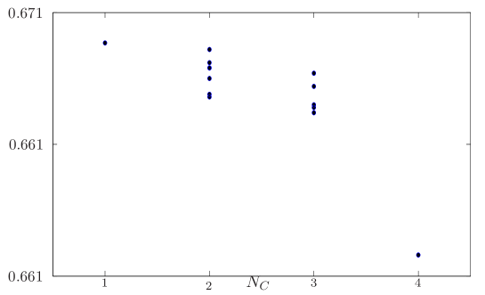
Figure 1: Mean square error $E(\|\tilde{x}_{10}\|^{2})$ versus number of clusters $N_{C}$ for every cluster configuration for the system with data given in (22).

Now let us introduce a more relevant change in one mode by replacing $A_{4}$, $G_{4}$, $L_{4}$ and $H_{4}$ with

$$10A_{4},10G_{4},10L_{4}\text{ and }10H_{4},$$ (23)

respectively. The results are displayed in Figure 2. We now can clearly distinguish two groups of filters, one with average errors around 106 and a second one around 104. In this setup, there is a tendency for better performance when $\theta=4$ is isolated from other states, e.g. with $S_{1}=\{1,2,3\}$ and $S_{2}=\{4\}$ we have $E(\|\tilde{x}_{10}\|^{2})\simeq 7,566.69$, while $S_{1}=\{1,2\}$ and $S_{2}=\{3,4\}$ lead to $E(\|\tilde{x}_{10}\|^{2})\simeq 1,286,306.18$. Moreover, considering that the (hard to implement) Kalman filter yields $E(\|\tilde{x}_{10}\|^{2})\simeq 5,152.95$ we see that the filter with configuration $S_{1}=\{1,2,3\}$ and $S_{2}=\{4\}$ is quite competitive in this scenario.

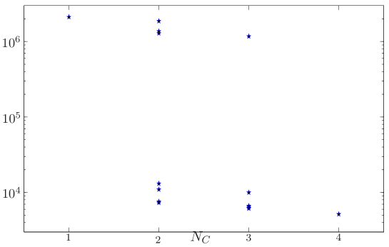
Figure 2: Mean square error $E(\|\tilde{x}_{10}\|^{2})$ versus number of clusters $N_{C}$ for every cluster configuration for the system with data given in (23).

6 Concluding remarks

We have explored the Markov state information structure in MJLS leading to new filters whose estimation error and complexity lie in the between the standard Kalman filter and the LMMSE, and establish a trade-off between performance and computational burden. This allows one to explore the computational resources at hands more deeply, seeking for the best possible estimates. As illustrated in the example, the new filters can provide competitive alternatives to the existing ones. We note that, for a given plant, the computational burden depends only on $N_{C}$, see the formulas given in Section 4.1. Then, a relevant question is how to select the Markov states to form each cluster so that the estimation error is minimized, which will be considered in future research.

References

- [1] Anderson, B. D. O., and Moore, J. B. Optimal Filtering, first ed. Prentice-Hall, London, 1979.
- [2] Costa, O. L., and Benites, G. R. Linear minimum mean square filter for discrete-time linear systems with Markov jumps and multiplicative noises. Automatica 47, 3 (2011), 466 – 476.
- [3] Costa, O. L. V. Linear minimum mean square error estimation for discrete-time Markovian jump linear systems. IEEE Transactions on Automatic Control 39, 8 (1994), 1685–1689.
- [4] Costa, O. L. V., Fragoso, M. D., and Marques, R. P. Discrete-Time Markovian Jump Linear Systems. Springer-Verlag, New York, 2005.
- [5] Fioravanti, A. R., Gonçalves, A. P., and Geromel, J. C. H2 filtering of discrete-time Markov jump linear systems through linear matrix inequalities. International Journal of Control 81, 8 (2008), 1221–1231.
- [6] Gonçalves, A. P., Fioravanti, A. R., and Geromel, J. C. Markov jump linear systems and filtering through network transmitted measurements. Signal Processing 90, 10 (2010), 2842 – 2850.
- [7] Miller, B. M., and Runggaldier, W. J. Kalman filtering for linear systems with coefficients driven by a hidden Markov jump process. Systems & Control Letters 31 (1997), 93–102.