Normal and superfluid fractions of inhomogeneous nonequilibrium quantum fluids

Abstract

We present a theoretical analysis of the normal and superfluid fractions of quantum fluids described by a nonequilibrium extension of the Gross-Pitaevskii equation in the presence of an external potential. Both disordered and regular potentials are considered. The normal and superfluid fractions are defined by the response of the nonequilibrium quantum fluid to a vector potential, in analogy with the equilibrium case. We find that the physical meaning of these definitions breaks down out of equilibrium. The normal and superfluid fractions no longer add up to one and for some types of external potentials, they can even become negative.

I Introduction

The hydrodynamic behavior of multimode laser systems has been recognized long ago Brambilla et al. (1991); Staliunas (1993), but it is on the platform of semiconductor exciton-polaritons that a systematic investigation of the hydrodynamics of photonic systems has been performed Carusotto and Ciuti (2013). Microcavity polaritons are hybrid light matter excitations in semiconductor heterostructures consisting of a quantum well embedded inside an optical microcavity Deveaud (2007). When the optical mode is resonant with the quantum well exciton frequency, the quasi-particles are the coherent superpositions of exciton and photon. Thanks to the photonic component, the microcavity polariton is much lighter than the bare exciton, which enhances the coherence properties. Thanks to the excitonic component, polaritons show a significant interaction strength. Being bosonic particles, microcavity polaritons can show long range phase coherence in the quantum degenerate regime, giving rise to superfluid Leggett (1999) properties, such as quantized vortices Lagoudakis et al. (2008).

The photonic component also introduces losses, which makes it so far impossible to achieve fully equilibrated Bose-Einstein condensation. In order to compensate for the finite polariton life time, particles have to be injected. The two main schemes are resonant and nonresonant excitation. In the former regime, the velocity of the polariton fluid can be tuned by varying the angle of the excitation laser. With this pumping scheme, superfluidity according to the Landau criterion (absence of scattering off defects) Amo et al. (2009) and the nucleation of quantized vortices Nardin et al. (2011) as well as solitons Amo et al. (2011) have been experimentally observed. Despite the finite polariton life time, the observed phenomenology in those experiments was close to the equilibrium behavior.

From a conceptual viewpoint, the main disadvantage of resonant excitation is the fact that the pumping laser fixes the phase of the quantum fluid, which excludes the study of superfluidity in the sense of linear response or metastable superflow. It has been argued Carusotto and Ciuti (2013) that the most precise and quantitative definition of superfluid $f_{s}$ and normal $f_{n}$ fractions involves the response of the quantum gas to a weak transverse vector potential ${\bf A}$ as analyzed in Ref. Hohenberg and Martin, 1965. For a spatially homogeneous system of density $n$, the normal fraction $f_{n}$ can be defined as

$$f_{n}=\lim_{q\to 0}\frac{m}{n}\chi_{T}({\bf q}).$$ (1)

Here $m$ is the effective mass and $\chi_{T}({\bf q})$ is the susceptibility tensor relating the average transverse current to the applied vector field in Fourier space.

The major question is here to what extent the nonequilibrium character of polariton condensates affects their superfluid properties. A first theoretical study was performed by Keeling on the superfluid fraction of a homogeneous driven-dissipative polariton condensate with a Keldysh functional integral approach Keeling (2011). Out of equilibrium, a nonvanishing normal component is always present, due to nonequilibrium fluctuations.

The work by Janot et al. Janot et al. (2013) addressed superfluidity in the disordered case. A reduction in superfluid fraction due to disorder is due to the pinning of the fluid in the potential minima and a first theoretical estimate can be obtained at the mean field level Lieb et al. (2002); Fontanesi et al. (2010). In the theoretical study of Ref. Janot et al., 2013, the response was studied to a small twist $\theta$ of the phase between two boundaries of the condensate separated by its size $L$. This is equivalent to the presence of a weak vector potential ${\bf A}={\bf e}_{x}\theta/L$. As argued in Ref. Janot et al., 2013, the superfluid stiffness in this case can be estimated in accordance with the equilibrium definitions Leggett (1970); Fisher et al. (1973) as

$$f_{s}=\frac{\omega(A)-\omega(0)}{A^{2}},$$ (2)

where $\hbar\omega$ is the chemical potential of the condensate.

The weak vector potential ${\bf A}={\bf e}_{x}\theta/L$ corresponds to a slow rotation at a velocity of less than one quantum of circulation $v<2\pi/L$. Due to the phase quantization, the superfluid cannot rotate, so that the current is supported by the normal phase only (Hess-Fairbank effect) Leggett (1999). This allows us to define the normal fraction in terms of the dependence of the current density on the gauge field

$$f_{n}=\frac{\langle j_{x}(A_{x})\rangle}{nA_{x}}.$$ (3)

The application of (synthetic) gauge fields in optical systems has developed into an active field of research Lu et al. (2014), thanks to several experimental breakthroughs Hafezi et al. (2011); Rechtsman et al. (2013a, b) and a wealth of theoretical proposals. Seen from this context, we address the question of the effect of a small gauge field on a the frequency and current in a nonequilibrium condensate.

II Model

We will apply the aforedescribed definitions of $f_{s}$ and $f_{n}$ to the systems described by the generalized Gross-Pitaevskii equation (gGPE) Wouters and Carusotto (2007); Keeling and Berloff (2008), which is taken in the form Carusotto and Ciuti (2013)

$$i\hbar\frac{\partial\psi}{\partial t}= \left[-\frac{\hbar^{2}\nabla^{2}}{2m}+g|\psi|^{2}+V\right.$$ (4)

$$\left.+\frac{i}{2}\left(\frac{P}{1+|\psi|^{2}/n_{s}}-\gamma\right)\right]\psi,$$

with a static potential $V({\bf r})$ and a contact interaction with the strength $g$. The imaginary term in the square brackets on the right hand side describes the saturable pumping (with strength $P$ and saturation density $n_{s}$), that compensates for the losses ($\gamma$). The physical origin of the pumping term for exciton-polariton condensates is an excitonic reservoir that is excited by a nonresonant laser.

In general, the pumping intensity $P$ is coordinate dependent and can be represented as $P({\bf r})=P_{0}p({\bf r})$, with $P_{0}=\max{P({\bf r})}$. Assuming that the interaction strength is positive, $g>0$, it is convenient to rewrite Eq. (4) in a dimensionless form, by expressing the particle density $|\psi|^{2}$ in units of $n_{0}\equiv n_{s}(P_{0}/\gamma-1)$, time in units of $\hbar/(gn_{0})$, and length in units of $\hbar/\sqrt{2mgn_{0}}$:

$$i\frac{\partial\psi}{\partial t}= \left[-\nabla^{2}+|\psi|^{2}+V_{0}v\phantom{\frac{\psi^{2}}{\psi^{2}}}\right.$$ (5)

$$\left.+ic\frac{1-|\psi|^{2}+(1+\nu^{-1})(p-1)}{1+\nu|\psi|^{2}}\right]\psi.$$

Equation (5) contains three dimensionless scalar parameters: $V_{0}=\max{|V({\bf r})|}/{gn_{0}}$, $c=\gamma/(2gn_{s})$ and $\nu=n_{0}/n_{s}$. The dimensionless functions $p({\bf r})$ and $v({\bf r})=V({\bf r})/(V_{0}gn_{0})$ describe the spatial distributions of the pumping intensity and static potential, respectively.

Our numerical simulations are performed for a region of sizes $L_{x}\times L_{y}$ with periodic boundary conditions in the $x$ direction and the Neumann boundary conditions at $y=0,L_{y}$. A uniform grid with $N_{x}\times N_{y}$ nodes is used. A vector potential, chosen as ${\bf A}=(A_{x},0,0)$ with constant $A_{x}$, is introduced by replacing $\partial/\partial x$ with $\partial/\partial x-iA_{x}$ in Eq. (5). For electrically charged particles, our configuration would correspond to a 2D cylindrical shell in an axially symmetric magnetic field parallel to the cylinder axis. We should keep in mind that in the case of an inhomogeneous static potential and/or pumping intensity, described by the functions $v({\bf r})$ and $p({\bf r})$, respectively, the average current $\langle j_{x}\rangle$ can be nonzero even at $A=0$. A natural generalization of the expression (3) for $f_{n}$ to this case seems to be

$$f_{n}=\frac{\langle j_{x}(A_{x})\rangle-\langle j_{x}(0)\rangle}{nA_{x}},$$ (6)

where the current density in the units used is given by the expression

$${\bf j}={\rm Im}\left[\psi^{*}\nabla\psi\right].$$ (7)

III Random potentials

Irregular potential landscapes are highly relevant for experimental realisations of polariton condensation because of growth imperfections in the semiconductor heterostructures. At equilibrium, the interplay between Bose-Einstein condensation and disorder gives rise to rich physics, with a zero temperature superfluid to Bose-glass quantum phase transitionFisher et al. (1989).

We consider the case of a uniform pumping intensity ($p({\bf r})=1$) and a static potential, described by a random distribution $v({\bf r})$. Two examples of the used random distributions, $v_{A}(x,y)$ and $v_{B}(x,y)$, with the correlation length $\xi_{v}=5$ and 3, respectively, are shown in Figs. 1a and 1b.

Figure 1: Distributions $v_{A}(x,y)$ (panel a) and $v_{B}(x,y)$ (panel b) for two random potentials with the correlation length $\xi_{v}=5$ and 3, respectively. (c) $f_{s}$ and $f_{n}$, calculated for $v=v_{A}$, $L_{x}=L_{y}=64$, $N_{x}=N_{y}=32$, $A_{x}=0.1$ and for $v=v_{B}$, $L_{x}=L_{y}=64$, $N_{x}=N_{y}=64$, $A_{x}=0.03$, as a function of $V_{0}$. Inset: $f_{s}$ and $f_{n}$, calculated for $v=v_{A}$, $L_{x}=L_{y}=64$, $N_{x}=N_{y}=32$, $V_{0}=0.24$, as a function of $A_{x}$. The calculations are performed for $\nu=1$, $c=1$, $p({\bf r})=1$.

In Fig. 1c we plot the quantities $f_{s}$ and $f_{n}$, corresponding to these potential distributions, as a function of the strength $V_{0}$ of the potential. In a qualitative agreement with the results of Ref. Janot et al., 2013, for both random potentials the function $f_{s}$ decreases with $V_{0}$ and falls to zero at a sufficiently strong potential. At the same time, in the whole range of $V_{0}$ under consideration, the calculated $f_{n}$ remains close to zero or even becomes negative at large $V_{0}$, so that the expected “sum rule” $f_{s}+f_{n}=1$ is obviously violated. At first sight, this violation could be related exclusively to the calculated $f_{n}$ (e.g., to lack of physical meaning of expression (6) or a lack of numerical accuracy in the corresponding estimation). However, a deeper analysis shows that the problem actually has a more general character. Indeed, from the inset to Fig. 1c one can see not only a pronounced asymmetry of $f_{n}(A_{x})$, which further illustrates inconsistencies in treating the found $f_{n}$ as the normal fraction of the condensate, but also the presence of a clear discontinuity of $f_{s}(A_{x})$ at $|A_{x}|\to 0$. The latter allows us to put under question also the possibility to interpret the calculated $f_{s}$ as the superfluid stiffness. In other words, in the presence of a random potential, neither Eq. (2) nor Eq. (6) seem to provide correct estimates for the superfluid and normal fractions of the condensate described by Eq. (5). This fact can be attributed to the existence of non-negligible in-plane currents in the condensates under consideration, even at $A=0$. Below we will illustrate the above statement by few simple examples with regular potentials.

IV Regular potentials

First, let us consider a structure with a partial cut in the direction perpendicular to the vector potential ${\bf e}_{x}A_{x}$. The cut is introduced through the additional condition $\left.\psi\right|_{x=L_{x}/2,y\leq L_{\rm cut}}=0$. An example of the density and current distributions in a system with such a cut, as given in Figs. 2a and 2b, respectively, corresponds to $V_{0}=0$, $p=1$, $c=1$ and $\nu=2$.

Figure 2: Density $|\psi|^{2}$ (panel a) and current $j_{x}$ (panel b) distributions, calculated for a system with $L_{x}=L_{y}=64$, $N_{x}=N_{y}=32$, $L_{\rm cut}=0.4L_{y}$, $V_{0}=0$, $p=1$ and $c=1$ at $\nu=2$, $A_{x}=0$. (c) $f_{s}$ and $f_{n}$, calculated for the same system at $A_{x}=0.05$, as a function of $\nu$.

At those parameter values the contribution of the pumping-loss term to gGPE is relatively large [see Eq. (5)] leading to the appearance of rather strong currents on both sides of the cut (see Fig. 2b). The corresponding values of $f_{s}$ and $f_{n}$ as well as their sum are significantly smaller than one (see Fig. 2c for $\nu\leq 2$). With increasing $\nu$, the role of the pumping-loss term is suppressed, equation (5) approaches the standard Gross-Pitaevskii equation, and the quantities $f_{s}$ and $f_{n}$ gradually restore their physical meaning, so that the sum $f_{s}+f_{n}$ tends to reach 1 at $\nu\sim 10$.

In Fig. 3 we show $f_{s}(V_{0})$ and $f_{n}(V_{0})$ calculated for a system, where the aforementioned cut is replaced with a potential well $V_{0}v(x)$, uniform in the $y$ direction (see the inset to Fig. 3).

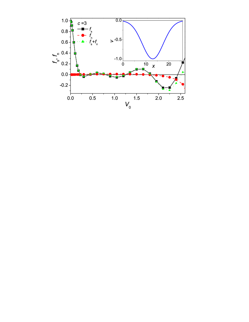
Figure 3: $f_{s}$ and $f_{n}$ as a function of $V_{0}$ for $L_{x}=26$, $N_{x}=128$, $c=3$, $\nu=2$, $p=1$, $A_{x}=0.04$. Inset: shape $v(x)$ of the static potential (solid line) and density distribution $|\psi(x)|^{2}$ at $V_{0}=0.45$ (dashed line).

Figure 3 corresponds to a relatively large value of the parameter $c$ ($c=3$). In this case, the behaviour of $f_{n}(V_{0})$ closely resembles that in the presence of a random static potential (Fig. 1c). The quantity $f_{s}(V_{0})$, shown in Fig. 3, first manifests a decrease, qualitatively similar to that in Fig. 1c. At larger $V_{0}$, this decrease is overridden by oscillations of $f_{s}(V_{0})$. Here, the definition (1) clearly loses its physical meaning of normal fraction.

The equality $f_{s}+f_{n}=1$ is seen to be satisfied only at $V_{0}\to 0$. Like in our previous example, when suppressing the pumping-loss term (in the present case this is realised by decreasing the parameter $c$) so that the system approaches an equilibrium regime, the behaviour of $f_{s}(V_{0})$ and $f_{n}(V_{0})$ becomes more reasonable (see Fig. 4). In particular, as seen from the inset to Fig. 4, the range of potential strengths $V_{0}$, where the condition $f_{s}+f_{n}=1$ is obeyed, increases clearly with decreasing $c$, so that at $c=0.03$ this range includes $V_{0}\sim 1$.

Figure 4: $f_{s}$ (panel a) and $f_{n}$ (panel b) as a function of $V_{0}$ for $L_{x}=26$, $N_{x}=128$, $\nu=2$, $p=1$, $A_{x}=0.04$ and different $c$. Inset: $f_{s}+f_{n}$ as a function of $V_{0}$.

In our last example we consider a system where a strong asymmetry is induced by an inhomogeneous pumping with the intensity maximum shifted with respect to the extrema of the potential $V_{0}v(x)$ (see Fig. 5a). The system is uniform in the $y$ direction. As displayed in Fig. 5b, the combined effect of the potential barrier and inhomogeneous pumping leads to a very non-uniform density distribution with strong currents, mainly in the positive $x$ direction. In Fig. 5c, at relatively small $V_{0}$, reasonable, nearly zero values of $f_{s}$ are accompanied by a counterintuitive decrease of $f_{n}$ with increasing the height $V_{0}$ of the potential barrier. At larger $V_{0}$, both $f_{s}(V_{0})$ and $f_{n}(V_{0})$ demonstrate some oscillatory behaviour, which can hardly have any physical meaning. One can also notice that the condition $f_{s}+f_{n}=1$ is not fully satisfied even at $V_{0}=0$.

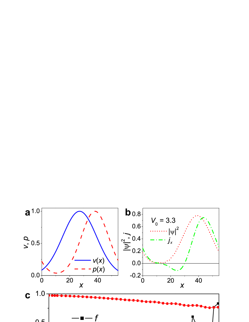
Figure 5: (a) Functions $v(x)$ (solid line) and $p(x)$ (dashed line), which determine the spatial distributions of the static potential and the pumping intensity, respectively, in a periodic system with $L_{x}=55$, $N_{x}=128$. (b) Distributions of the density $|\psi|^{2}$ (dotted line) and current density $j_{x}$ (dash-dotted line) at $\nu=3$, $c=4$, and $V_{0}=3.3$. (c) $f_{s}$ and $f_{n}$, calculated for $\nu=3$, $c=4$, $A_{x}=0.035$, as a function of $V_{0}$. Panels d and e show $f_{s}$ and $f_{n}$, respectively, as a function of $A_{x}$ for $\nu=3$, $c=4$ and three different $V_{0}$.

As seen from Fig. 5d, at sufficiently large $V_{0}$, the calculated function of $f_{s}(A_{x})$ can have a pronounced discontinuity at $|A_{x}|\to 0$, which is similar to that shown in the inset to Fig. 1c for the case of a random static potential. The origin of this discontinuity can be qualitatively understood by associating the presence of a nonzero average current in the system at $A_{x}=0$ with an effective vector potential $A_{0x}\neq 0$. Then, assuming like before that the chemical potential of the superfluid is proportional to the vector potential squared, $\omega(A)=\alpha A^{2}$, one obtains from Eq. (2) the expression $f_{s}=(1+2A_{0x}/A_{x})\alpha$, which obviously diverges at $|A_{x}|\to 0$. The existence of a nonzero average current in the absence of an externally applied vector potential seems to be responsible also for the asymmetry of the calculated function $f_{n}(A_{x})$ at large $V_{0}$, both in the present example (see Fig. 5e) and in the case of a random potential (see the inset in Fig. 1c).

V Conclusions

Summarising our numerical findings, we can conclude that the definitions (1) and (2) lose their physical interpretation in terms of normal and superfluid fractions in the presence of driving and decay. For what concerns the definition of the superfluid fraction (2), this may not be that surprising, since the stationary state is no longer the one with minimal (free) energy. For the case of a disordered potential, however, the superfluid fraction shows an expected behavior as a function of disorder strength, starting from one at zero disorder and falling to zero for stronger disorder.

For other potential profiles however, such as a single potential dip, the equilibrium definition of the superfluid fraction becomes problematic. It becomes negative for certain values of the potential. This means the frequency of the condensate shows a decrease instead of an increase under the application of a phase twist in the boundary condition. In equilibrium, this is forbidden, since time reversal invariance guarantees that the condensate wave function in the ground state is real. Out of equilibrium, where time reversal invariance is broken, the steady state also has currents for periodic boundary conditions. The interplay between this existing current and the applied phase twist can then lead to a lower frequency. In the case of a spatially inhomogeneous pump, the behavior of the superfluid fraction even differs more dramatically from the equilibrium one, showing large oscillations as function of the external potential strength (see Fig. 5c).

At first, the definition of the normal fraction, based on the current response of the system, could be thought to be more robust with respect to the nonequilibrium condition. Our numerical analysis however strongly contradicts this. Already in the case of the disordered potential, where the superfluid fraction behaves reasonably, the normal fraction does not show the expected behavior. We also attribute the failure of the equilibrium definition of the superfluid fraction to the presence of currents in the steady state. These currents invalidate the physical picture that the current response is due to a limited stiffness of the condensate phase. When currents are present in the steady state, also a redistribution of the density will contribute to the current response. The interplay between the density redistribution and the steady state currents can then even lead to negative normal fraction, as we observed in the case of the disordered potential landscape (Fig. 1c). The conclusion of our numerical findings is negative: the equilibrium definitions for superfluid and normal fractions no longer give meaningful results out of equilibrium in the presence of external potentials that induce currents.

It will be of interest to include the effect of fluctuations in the calculation of the superfluid and normal fractions. Within the classical field formalism, this could be done in the truncated Wigner approximation Wouters and Savona (2009). Of specific interest are the superfluid and normal fraction close to the phase transition. At equilibrium, it is of the BKT type in two dimensions, with a characteristic jump in the superfluid fraction. Indications that the BKT character of the phase transition is preserved out of equilibrium were found recently in numerical simulations in the parametric oscillation regime Dagvadorj et al. (2015), but the behavior of the normal and superfluid fractions has not been addressed yet.

References

- Brambilla et al. (1991) M. Brambilla, L. A. Lugiato, V. Penna, F. Prati, C. Tamm, and C. O. Weiss, Phys. Rev. A 43, 5114 (1991).
- Staliunas (1993) K. Staliunas, Phys. Rev. A 48, 1573 (1993).
- Carusotto and Ciuti (2013) I. Carusotto and C. Ciuti, Rev. Mod. Phys. 85, 299 (2013).
- Deveaud (2007) B. Deveaud, The physics of semiconductor microcavities (John Wiley & Sons, 2007).
- Leggett (1999) A. J. Leggett, Rev. Mod. Phys. 71, S318 (1999).
- Lagoudakis et al. (2008) K. G. Lagoudakis, M. Wouters, M. Richard, A. Baas, I. Carusotto, R. André, L. S. Dang, and B. Deveaud-Plédran, Nature Physics 4, 706 (2008).
- Amo et al. (2009) A. Amo, J. Lefrère, S. Pigeon, C. Adrados, C. Ciuti, I. Carusotto, R. Houdré, E. Giacobino, and A. Bramati, Nature Physics 5, 805 (2009).
- Nardin et al. (2011) G. Nardin, G. Grosso, Y. Léger, B. Piȩtka, F. Morier-Genoud, and B. Deveaud-Plédran, Nature Physics 7, 635 (2011).
- Amo et al. (2011) A. Amo, S. Pigeon, D. Sanvitto, V. Sala, R. Hivet, I. Carusotto, F. Pisanello, G. Leménager, R. Houdré, E. Giacobino, et al., Science 332, 1167 (2011).
- Hohenberg and Martin (1965) P. Hohenberg and P. Martin, Annals of Physics 34, 291 (1965).
- Keeling (2011) J. Keeling, Phys. Rev. Lett. 107, 080402 (2011).
- Janot et al. (2013) A. Janot, T. Hyart, P. R. Eastham, and B. Rosenow, Phys. Rev. Lett. 111, 230403 (2013).
- Lieb et al. (2002) E. H. Lieb, R. Seiringer, and J. Yngvason, Phys. Rev. B 66, 134529 (2002).
- Fontanesi et al. (2010) L. Fontanesi, M. Wouters, and V. Savona, Phys. Rev. A 81, 053603 (2010).
- Leggett (1970) A. J. Leggett, Phys. Rev. Lett. 25, 1543 (1970).
- Fisher et al. (1973) M. E. Fisher, M. N. Barber, and D. Jasnow, Phys. Rev. A 8, 1111 (1973).
- Lu et al. (2014) L. Lu, J. D. Joannopoulos, and M. Soljačić, Nature Photonics (2014).
- Hafezi et al. (2011) M. Hafezi, E. A. Demler, M. D. Lukin, and J. M. Taylor, Nature Physics 7, 907 (2011).
- Rechtsman et al. (2013a) M. C. Rechtsman, J. M. Zeuner, A. Tünnermann, S. Nolte, M. Segev, and A. Szameit, Nature Photonics 7, 153 (2013a).
- Rechtsman et al. (2013b) M. C. Rechtsman, J. M. Zeuner, Y. Plotnik, Y. Lumer, D. Podolsky, F. Dreisow, S. Nolte, M. Segev, and A. Szameit, Nature 496, 196 (2013b).
- Wouters and Carusotto (2007) M. Wouters and I. Carusotto, Phys. Rev. Lett. 99, 140402 (2007).
- Keeling and Berloff (2008) J. Keeling and N. G. Berloff, Phys. Rev. Lett. 100, 250401 (2008).
- Fisher et al. (1989) M. P. A. Fisher, P. B. Weichman, G. Grinstein, and D. S. Fisher, Phys. Rev. B 40, 546 (1989).
- Wouters and Savona (2009) M. Wouters and V. Savona, Phys. Rev. B 79, 165302 (2009).
- Dagvadorj et al. (2015) G. Dagvadorj, J. M. Fellows, S. Matyjaśkiewicz, F. M. Marchetti, I. Carusotto, and M. H. Szymańska, Phys. Rev. X 5, 041028 (2015).