Test particles in a magnetized conformastatic spacetime

Abstract

A class of exact conformastatic solutions of the Einstein-Maxwell field equations is presented in which the gravitational and electromagnetic potentials are completely determined by a harmonic function. We derive the equations of motion for neutral and charged particles in a spacetime background characterized by this class of solutions. As an example, we focus on the analysis of a particular harmonic function, which generates a singularity-free and asymptotically flat spacetime that describes the gravitational field of a punctual mass endowed with a magnetic field. In this particular case, we investigate the main physical properties of equatorial circular orbits. We show that due to the electromagnetic interaction, it is possible to have charged test particles which stay at rest with respect to a static observer located at infinity. Additionally, we obtain an analytic expression for the perihelion advance of test particles, and the corresponding explicit value in the case of a punctual magnetic mass. We show that the analytical expressions obtained from our analysis are sufficient for being confronted with observations, in order to establish whether such objects can exist in Nature.

I Introduction

In recent years, the interest in studying magnetic fields has increased in both astrophysics and cosmology. In astrophysical dynamics, the study of disk sources for stationary axially symmetric spacetimes with magnetic fields is of special relevance mainly on the investigation of neutron stars, white dwarfs, and galaxy formation. In this context, usually, it is believed that electric fields do not have a clear astrophysical importance; nevertheless, there is a possibility that some galaxies are positively charged González et al. (2008); Bally and Harrison (1978). On the other hand, magnetic fields are very common in astrophysical objects, and can drastically affect other physical properties (e.g, H-alpha emission, density mass, local shocks, etc.). For instance, magnetic fields in a galaxy can be measured from the non-thermal radio emission under the assumption of equipartition between the energies of the magnetic field and the relativistic particles (the so-called energy equipartition); this interaction can play an important role on the formation of arms in spiral galaxies (Uyaniker et al., 2004). For nearby galaxies, one can use other effects such as optical polarization, polarized emission of clouds and dust grains, maser emissions, diffuse radio polarized emission and rotation measures of background polarization sources as well. In the case of the Milky Way, e.g., the magnetic field has been actively studied in its three main regions (central bulge, halo and disk). Moreover, magnetic fields seem to play an important role on the formation of jets (resulting from collimated bipolar out flows of relativistic particles) and accretion disks near black holes and neutron stars (Zamaninasab et al., 2014).

It is important to stress that magnetic fields are found mainly on interstellar medium, remarkably, in spiral galaxies (Han, 2012) which can be described with a good approximation by means of thin disks. The magnetic and gravitational field of such objects can reach very high values. In a series of recent works (Gutiérrez-Piñeres, 2015; Guti rrez-Pi eres and Capistrano, 2015; Gutiérrez-Piñeres et al., 2015), several classes of static and stationary axisymmetric exact solutions of the Einstein-Maxwell equations were derived, which can be interpreted as describing the gravitational and magnetic fields of static and rotating thin disks. Although these solutions satisfy the main theoretical conditions to be considered as physically meaningful, additional tests are necessary in order to establish their applicability in realistic scenarios. For instance, the study of the motion of test particles and the comparison of the resulting theoretical predictions with observations are essential to understand the physical properties of the solutions and the free parameters entering them. This is the main goal of the present work.

To investigate the gravitational field of isolated non-spherical bodies, axial symmetry is usually assumed. This is a very reasonable and physically meaningful assumption. Nevertheless, it is clear that Nature does not choose a particular symmetry, but, instead, we assume symmetries in order to simplify the mathematical difficulties that are normally found when trying to find exact solutions for the description of gravitational fields. To investigate the possibility of having conformally symmetric compact objects in Nature, we explore in this work one of the simplest conformsymmetric solutions for an isolated body endowed with a magnetic field. We will see, in fact, that the resulting effects are enough to determine whether an isolated body belongs to the general class of axisymmetric compact objects or to its subclass of conformsymmetric objects.

In this work, we follow the original terminology introduced by Synge (Synge, 1960), according to which conformastationary spacetimes are stationary spacetimes with a conformally flat space of orbits, and conformastatic spacetimes comprises the static subset. In a previous work (Gutiérrez-Piñeres and Capistrano, 2015), a static conformastatic solution of Einstein-Maxwell equations was presented and, in particular, the corresponding geodesic equations were derived explicitly. In the present work, we perform a detailed analysis of the equations of motion of test particles moving in a conformastatic spacetime, which describes the gravitational and magnetic fields of a punctual source. In particular, we analyze the physical properties of circular orbits on the equatorial plane of the gravitational source. Additionally, we find an expression for the perihelion advance in a general magnetized conformastatic spacetime.

This work is inspired by the approach presented in references (Pugliese et al., 2011a) and (Pugliese et al., 2011b). The analysis presented here serves as a “proof-of-principle" that gives a solid footing for a fuller study of particles motion in the field of relativistic disks and for a later study in even more realistic astrophysical context.

This work is organized as follows. In Section II, we present the general line element for conformastatic gravitational fields which is a particular case of the general axisymmetric static line element. The Einstein-Maxwell equations are calculated explicitly and we show that there exists a class of solutions generated by harmonic functions. Moreover, we derive the complete set of differential equations and first integrals that govern the dynamics of charged test particles moving in a conformastatic spacetime. In addition, we show that, due to the spacetime symmetries, the geodesic equations on the equatorial plane can be reduced to one single ordinary differential equation, describing the motion of a particle in an effective potential, which depends on the radial coordinate only. In Section III, we derive the explicit expressions for the energy and angular momentum of a particle moving along a circular orbit. In Section IV, we focus on the particular case of a punctual source. We analyze all the physical and stability properties of circular orbits along which charged test particles are moving. In Section V, we obtain an expression for the perihelion advance of a charged test particle in a generic conformastatic spacetime in the presence of a magnetic field. In this section, we also consider the particular case of a punctual source to obtain concrete results that are confronted with the ones obtained in Einstein gravity alone. Finally, in Section VI, we present the conclusions.

II Basic framework

In Einstein-Maxwell gravity theory, a particular class of a gravitational fields can be described by the conformastatic metric in cylindrical coordinates (Gutiérrez-Piñeres et al., 2013)

$$ds^{2}=-c^{2}e^{2\phi}dt^{2}+e^{-2\phi}(dr^{2}+dz^{2}+r^{2}d\varphi^{2}),$$ (1)

where $c$ is the speed of light in vacuum and the metric potential $\phi$ depends only on the variables $r$ and $z$. This represents a subclass of the axisymmetric static Weyl class of gravitational fields. The field equations are the Einstein-Maxwell equations

$$R_{\alpha\beta}-\frac{1}{2}g_{\alpha\beta}R=k_{{}_{0}}E_{\alpha\beta},\quad\nabla_{\beta}F^{\alpha\beta}=0,$$ (2)

where $k_{{}_{0}}=8\pi\$G c^-4 . The energy-momentum tensor $E_{\alpha\beta}$ is given by

$$E_{\alpha\beta}=\frac{1}{4\pi}\left\{F_{\alpha\gamma}F_{\beta}^{\;\;\gamma}-\frac{1}{4}g_{\alpha\beta}F_{\gamma\delta}F^{\gamma\delta}\right\},$$

where the electromagnetic tensor is denoted by $F_{\alpha\beta}=A_{\beta,\alpha}-A_{\alpha\beta}$, being $A_{\alpha}=(A_{t},\mathbf{A})$ the electromagnetic four-potential. The components of the electromagnetic four-potential depend on $r$ and $z$ only.

For the sake of simplicity, we suppose that the only nonzero component of the four-potential is $A_{\varphi}$. From a physical point of view, this means that we will limit ourselves to the analysis of magnetic fields only; electric fields are supposed to be negligible. This is also in accordance with the general believe that electric fields are not of importance in astrophysics, as mentioned in the Introduction. In general, electrovacuum axisymmetric static spacetimes are considered either with electric, magnetic or both fields Stephani et al. (2009); no restriction needs to be imposed in this case. In the subclass of conformastatic fields, it is also possible to consider electric and magnetic fields simultaneously (Gutiérrez-Piñeres et al., 2015); nevertheless, the physical interpretation of the solutions in this case is more involved. In reference (Guti rrez-Pi eres and Capistrano, 2015), for instance, this kind of solutions has been interpreted in terms of magnetized halos around thin disks. As we will see below, the restriction to only the magnetic component of the four-potential allows us to describe the gravitational field of compact objects endowed with magnetic fields.

In fact, the assumption that only $A_{\varphi}$ is non-vanishing drastically reduces the complexity of the Einstein-Maxwell equations (2), which can be equivalently written as

$$\nabla^{2}\phi=\nabla\phi\cdot\nabla\phi,$$ (3)

$$\phi_{,r}^{\,2}=\frac{G}{c^{4}r^{2}}e^{2\phi}A_{\varphi,z}^{2},$$ (4)

$$\phi_{,z}^{\,2}=\frac{G}{c^{4}r^{2}}e^{2\phi}A_{\varphi,r}^{2},$$ (5)

$$\phi_{,r}\phi_{,z}=-\frac{G}{c^{4}r^{2}}e^{2\phi}A_{\varphi,r}A_{\varphi,z},$$ (6)

$$\nabla\cdot(r^{-2}e^{2\phi}\nabla{A_{\varphi}})=0,$$ (7)

where $\nabla$ denotes the usual gradient operator in cylindrical coordinates, and a comma indicates partial differentiation with respect to the corresponding variable. The symmetry properties of the above differential equations allows us to reduce them to a single equation. In fact, by supposing a solution in the functional form $\phi=\phi[U(r,z)]$, where $U(r,z)$ is an arbitrary harmonic function restricted by the condition $U<1$ for all $r$ and $z$ (Gutiérrez-Piñeres et al. (2013), Gutiérrez-Piñeres (2015)), it is not difficult to prove that

$$\phi=-\ln{(1-U)},\quad A_{\varphi}(r,z)=\frac{c^{2}}{G^{1/2}}{\int_{0}^{r}{\tilde{r}U({\tilde{r},z}}})d\tilde{r},$$ (8)

represent a solution of the system (3).

The electromagnetic field is pure magnetic. This can be demonstrated by analyzing the electromagnetic invariant ${\cal F}=F^{\alpha\beta}F_{\alpha\beta}$, which in this case has the form

$${\cal F}\equiv F^{\alpha\beta}F_{\alpha\beta}=\frac{2c^{4}(U^{2}_{,r}+U^{2}_{,z})}{G(1-U)^{4}}\geq 0.$$ (9)

In fact, the nonzero components of the electromagnetic field are

$$B_{r}=\frac{c^{2}}{G^{1/2}}rU_{,r}\quad\text{and}\quad B_{z}=\frac{c^{2}}{G^{1/2}}rU_{,z}\ .$$ (10)

We conclude that any harmonic function $U(r,z)<1$ can be used to construct an exact conformastatic solution of the Einstein-Maxwell equations. This is an interesting result which allows us to investigate the physical properties of concrete conformastatic spacetimes. Indeed, in the sections below we will investigate, as a particular example, one of the simplest harmonic solutions which turns out to describe the gravitational field of a punctual mass.

We now analyze the geodesic equations for a general case. The motion of a test particle of mass $m$ and charge $q$ moving in a conformastatic spacetime given by the line element (1) is described by the Lagrangian

$${\cal L}=\frac{1}{2}mg_{\alpha\beta}\dot{x}^{\alpha}\dot{x}^{\beta}+\frac{q}{c}A_{\alpha}\dot{x}^{\alpha},$$ (11)

where a dot represents differentiation with respect to the proper time. The equations of motion of the test particle can be derived from the Lagrangian (11) by using the Hamilton equations

$$\dot{p}_{\alpha}=-\frac{\partial\cal{H}}{\partial{x}^{\alpha}},\quad\dot{x}_{\alpha}=\frac{\partial\cal{H}}{\partial{p}^{\alpha}},$$

$${\cal H}=\dot{x}^{\alpha}p_{\alpha}-{\cal L}\ ,\quad p_{\alpha}=\frac{\partial\cal{L}}{\partial\dot{x}^{\alpha}},$$ (12)

where $p_{\alpha}$ and $\cal H$ are the momentum and Hamiltonian of the particle, respectively. The coupled differential equations (12) for the Lagrangian (11) are very difficult to solve directly by using an analytic approach. However, we can use the symmetry properties of the conformastatic field to find first integrals of the motion equations which reduce the number of independent equations. This is the approach we will use below.

Since the Lagrangian (11) does not depend explicitly on the variables $t$ and $\varphi$, one can obtain the following two conserved quantities

$$p_{t}=-mce^{2\phi}\dot{t}\equiv-\frac{E}{c},$$ (13)

and

$$p_{\varphi}=mr^{2}e^{-2\phi}\dot{\varphi}+\frac{q}{c}{}A_{\varphi}\equiv L,$$ (14)

where $E$ and $L$ are, respectively, the energy and the angular momentum of the particle as measured by an observer at rest at infinity. Furthermore, the momentum $p_{\alpha}$ of the particle can be normalized so that $g_{\alpha\beta}\dot{x}^{\alpha}\dot{x}^{\beta}=-\Sigma$. Accordingly, for the metric (1) we have

$$-{c^{2}e^{2\phi}\dot{t}^{2}}+e^{-2\phi}(\dot{r}^{2}+\dot{z}^{2}+r^{2}\dot{\varphi}^{2})=-\Sigma,$$ (15)

where $\Sigma=0,c^{2},-c^{2}$ for null, time-like and space-like curves, respectively.

The relations (13), (14) and (15) give us three linear differential equations, involving the four unknowns $\dot{x}^{\alpha}$. It is possible to study the motion of test particles with only these relations, if we limit ourselves to the particular case of equatorial trajectories, i. e. $z=0$. Indeed, since the gravitational configuration is symmetric with respect to the equatorial plane, a particle with initial state $z=0$ and $\dot{z}=0$ will remain confined to the equatorial plane which is, therefore, a geodesic plane. Substituting the conserved quantities (13) and (14) into Eq.(15), we find

$$\dot{r}^{2}+\Phi=\frac{E^{2}}{m^{2}c^{2}},$$ (16)

where

$$\Phi(r)\equiv\frac{L^{2}}{m^{2}r^{2}}\left(1-\frac{qA_{\varphi}}{Lc}\right)^{2}e^{4\phi}+\Sigma e^{2\phi}$$ (17)

is an effective potential.

III Circular orbits

The motion of charged test particles is governed by the behavior of the effective potential (17). The radius of circular orbits and the corresponding values of the energy $E$ and angular momentum $L$ are given by the extrema of the function $\Phi$. Therefore, the conditions for the occurrence of circular orbits are

$$\frac{d\Phi}{dr}=0,\quad\Phi=\frac{E^{2}}{m^{2}c^{2}}.$$ (18)

We assume the convention that the positive value of the energy corresponds to the positivity of the solution $E_{\pm}=\pm mc\Phi^{1/2}$. Consequently, $E_{+}=-E_{-}=mc\Phi^{1/2}$.

Calculating the condition (18) for the effective potential (17), we find the angular momentum of the particle in circular motion

$$L_{c\pm}=\frac{qA_{\varphi}}{c}+\frac{qrA_{\varphi,r}e^{\phi}\pm\sqrt{\left(qrA_{\varphi,r}e^{\phi}\right)^{2}-4\Sigma c^{2}m^{2}r^{3}\phi_{,r}\left(2r\phi_{,r}-1\right)}}{2ce^{\phi}\left(2r\phi_{,r}-1\right)}.$$ (19)

Conventionally, we can associate the plus and minus signs in the subscript of the notation $L_{c\pm}$ to dextrorotation and levorotation, respectively.

Furthermore, by inserting the value of the angular momentum (19) into the second equation of Eq.(18), we obtain the energy $E_{\quad c\pm}^{(\pm)}$ of the particle in a circular orbit as

$$E_{\quad c\pm}^{(\pm)}=\pm\,mce^{\phi}\left(\Sigma+\xi^{(\pm)}_{\quad c}\right)^{1/2},$$ (20)

where

$$\xi^{(\pm)}_{\quad c}=\frac{\left[qrA_{\varphi,r}e^{\phi}\pm\sqrt{\left(qrA_{\varphi,r}e^{\phi}\right)^{2}-4\Sigma c^{2}m^{2}r^{3}\phi_{,r}\left(2r\phi_{,r}-1\right)}\right]^{2}}{4m^{2}c^{2}r^{2}\left(2r\phi_{,r}-1\right)^{2}}.$$ (21)

Therefore, each sign of the value of the energy corresponds to two kinds of motion (dextrorotation and levorotation) indicated in (20) and (21) by the superscripts $(\pm)$.

An interesting particular orbit is that one in which the particle is located at rest $(r_{r})$ as seen by an observer at infinity, i.e. $L=0$. These orbits are therefore characterized by the conditions

$$L=0,\quad\frac{d\Phi}{dr}=0.$$ (22)

For the metric (1) these conditions give us the following equation

$$\frac{2e^{2\phi}}{m^{2}c^{2}r^{3}}\left[q^{2}A_{\varphi}\left(2rA_{\varphi}\phi_{,r}+rA_{\varphi,r}-A_{\varphi}\right)e^{2\phi}+\Sigma m^{2}c^{2}r^{3}\phi_{,r}\right]=0\ .$$ (23)

To find the value of the rest radius $r_{r}$, we must solve Eq.(23).

Notice that from Eqs. (23) and (20) it follows that if $e^{2\phi}=0$ for an orbit with a rest radius $r=r_{r}$, the energy of the particle is $E_{r}=0$. In the case $e^{2\phi}\neq 0$, we have

$$E_{\quad r\pm}^{(\pm)}=\pm mce^{\phi}\left(\Sigma+\xi^{(\pm)}_{r}\right)^{1/2},$$ (24)

where

$$\xi^{(\pm)}_{\quad r}=\frac{q^{2}e^{2\phi}\left[rA_{\varphi,r}\pm\left(rA_{\varphi,r}+2A_{\varphi}\left(2r\phi_{,r}-1\right)\right)\right]^{2}}{4m^{2}c^{2}r^{2}\left(2r\phi_{,r}-1\right)^{2}}.$$ (25)

This analysis indicates that it is possible to have a test particle at rest with zero angular momentum ($L=0)$ and non-zero energy $(E_{r}\neq 0)$. This is a non-trivial effect that in the case of vanishing magnetic field has been associated with the existence of repulsive gravitational effects in Einstein gravity (Pugliese et al., 2011a).

The minimum radius for a stable circular orbit corresponds to an inflection point of the effective potential function. Thus, we must solve the equation

$$\frac{d^{2}\Phi}{dr^{2}}=0,$$ (26)

under the condition that the angular momentum is given by Eq.(19). From Eqs.(18) and (26), we find that the radius and angular momentum of the last stable circular orbit are related by the following equations

$$\frac{2e^{4\phi}}{m^{2}c^{2}r^{4}}\Big{[}(Lc-qA_{\varphi})^{2}\left(8r^{2}\phi_{,r}^{2}+2r^{2}\phi_{,rr}-8r\phi_{,r}+3\right)$$

$$+(Lc-qA_{\varphi})\left(-8qr^{2}A_{\varphi,r}\phi_{,r}-qr^{2}A_{\varphi,rr}+4qrA_{\varphi,r}\right)$$

$$+q^{2}r^{2}A_{\varphi,r}^{2}e^{2\phi}+2c^{2}\Sigma m^{2}r^{4}\phi_{,r}^{2}+c^{2}\Sigma m^{2}r^{4}\phi_{,rr}\Big{]}=0,$$ (27)

and

$$\frac{2e^{2\phi}}{m^{2}c^{2}r^{3}}\Big{[}e^{2\phi}(Lc-qA_{\varphi})\Big{(}(Lc-qA_{\varphi})(2r\phi_{,r}-1)-qrA_{\varphi,r}\Big{)}$$

$$+\;\Sigma m^{2}c^{2}r^{3}\phi_{,r}\Big{]}=0.$$ (28)

It is possible to solve Eq.(28) with respect to the stable circular orbit radius which then becomes a function of the free parameter $L$. Alternatively, from Eq. (27 ) we find the expression

$$L^{\pm}_{lsco} = \frac{qA_{\varphi}}{c}+\Bigg{\{}qe^{\phi}\left(8r^{2}A_{\varphi,r}\phi_{,r}^{2}+r^{2}A_{\varphi,rr}-4rA_{\varphi,r}\right)$$ (29)

$$\pm\Bigg{[}q^{2}e^{2\phi}\left(8r^{2}A_{\varphi,r}\phi_{,r}^{2}+r^{2}A_{\varphi,rr}-4rA_{\varphi,r}\right)^{2}$$

$$-4(q^{2}r^{2}A_{\varphi,r}^{2}e^{2\phi}+2c^{2}\Sigma m^{2}r^{4}\phi_{,r}^{2}+c^{2}\Sigma m^{2}r^{4}\phi_{,rr})$$

$$\times(8r^{2}\phi_{,r}^{2}+2r^{2}\phi_{,rr}-8r\phi_{,r}+3)\Bigg{]}^{1/2}\Bigg{\}}$$

$$\times\left[2ce^{\phi}(8r^{2}\phi_{,r}^{2}+2r^{2}\phi_{,rr}-8r\phi_{,r}+3)\right]^{-1}$$

for the angular momentum of the last stable circular orbit. Equation (29) can then be substituted in Eq. (28) to find the radius of the last stable circular orbit.

In this section, we found the expressions for the physical quantities which characterize the behavior of a charged test particle, moving along a circular trajectory in the gravitational field of a conformastatic mass distribution endowed with a magnetic field. These results are completely general, and can be applied to any solution of the corresponding Einstein-Maxwell equations.

IV The field of a punctual mass in Einstein-Maxwell gravity

We now illustrate the results obtained in the precedent section, focusing on the main physical properties of test particles moving along circular orbits. As shown before, the class of harmonic conformastatic solutions is of particular interest, because all the metric components and the magnetic field are defined in terms of a single harmonic function. Let us consider one of the simplest harmonic functions which in Newtonian gravity would describe the gravitational field of a punctual mass, namely,

$$U(r,z)=-\frac{GM}{c^{2}R},\quad R^{2}=r^{2}+z^{2}\ ,$$ (30)

where $M$ is a real constant. According to Eq.(8), for the metric and electromagnetic potentials we have

$$\phi(r,z)=-\ln{\left(1+\frac{GM}{c^{2}R}\right)}\ ,$$ (31)

and

$$A_{\varphi}(r,z)=\sqrt{G}M\left(1-\frac{z}{R}\right)\ ,$$ (32)

respectively. At spatial infinity, the magnetic potential is non-zero and constant, except at the symmetry axis where it vanishes. Notice also that on the equatorial plane the magnetic potential is constant everywhere. As for the metric potential, its physical significance can be investigated by considering the asymptotic behavior of the metric component $g_{tt}$ for which we obtain

$$\lim_{R\to\infty}g_{tt}(r,z)\approx-1+\frac{2GM}{c^{2}R}-\frac{3G^{2}M^{2}}{c^{4}R^{2}}+{\cal O}\left(\frac{1}{R^{3}}\right)\ .$$ (33)

Accordingly, this particular solution can be interpreted as describing the gravitational field of a punctual mass on the background of a magnetic field. In the limiting case $M\rightarrow 0$, we obtain the Minkowski spacetime, indicating that $M$ is the source of the gravitational and the magnetic field as well. This result can be corroborated by analyzing the Kretschmann scalar ${\cal K}=R_{\alpha\beta\gamma\delta}R^{\alpha\beta\gamma\delta}$ and the electromagnetic invariant $\cal F$ (see Eq.(9)) which in this case have the following expressions

$${\cal K}=\frac{8M^{2}c^{8}G^{2}(G^{2}M^{2}+6c^{4}R^{2})}{(c^{2}R+GM)^{8}},$$ (34)

and

$${\cal F}=\frac{2GM^{2}c^{8}}{(c^{2}R+GM)^{4}},$$ (35)

respectively. In addition, from the expressions (33), ( 34) and (35), we conclude that the gravitational field is asymptotically Schwarzschild-like and singularity-free.

The field lines of the magnetic field are given by the ordinary differential equation ${dr}{B_{z}}={dz}{B_{r}}.$ Moreover, the nonzero components of the magnetic field are $B_{r}=G^{1/2}Mr^{2}R^{-3}$ and $B_{z}=G^{1/2}MrzR^{-3}$ . Thus, we see that the equation

$$z^{2}=\frac{\left(1-\gamma\right)^{2}}{\gamma(2-\gamma)}r^{2}\ ,$$ (36)

where $0<\gamma<2$, represents the lines of force of the magnetic field. The components of the magnetic field vanish at spatial infinity, and diverge at the origin $R=0$. This, however, is not a true singularity as can be seen from the expression for the electromagnetic invariant (35). In Fig.1, we illustrate the spatial behavior of the lines of force of this magnetic configuration. It shows that the source of the magnetic field coincides with the punctual mass, in accordance with the analytic expressions for the gravitational and magnetic potentials.

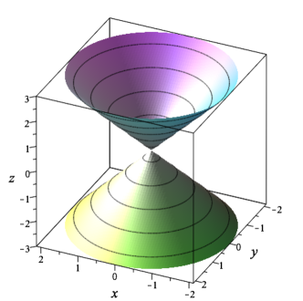
Figure 1: Illustration of the spatial distribution of the magnetic lines of force of a punctual conformastatic source located at the origin of coordinates.

IV.1 Circular motion of a charged test particle

Consider the case of a charged particle moving in the conformastatic field of a punctual mass given by Eqs. (31) and (32). This means that we are considering the motion described by the following effective potential

$$\Phi(r)=\frac{c^{6}r^{2}(Lc-q\sqrt{G}M)^{2}}{m^{2}(c^{2}r+GM)^{4}}+\frac{\Sigma c^{4}r^{2}}{(c^{2}r+GM)^{2}}.$$ (37)

We note that

$$e^{\phi(r)}=\frac{c^{2}r}{c^{2}r+GM}$$ (38)

on the equatorial plane.

According to the general results of the previous section, the angular momentum and the energy for a circular orbit with radius $r_{c}$ are given by

$$L_{c\;\pm}=\frac{q\sqrt{G}M}{c}\mp\frac{(c^{2}r_{c}+GM)m}{c^{2}}\sqrt{\frac{\Sigma GM}{c^{2}r_{c}-GM}}$$ (39)

and

$$E_{c\;\pm}=\pm\frac{mc^{4}}{\left(c^{2}r_{c}+GM\right)}\sqrt{\frac{\Sigma r_{c}^{3}}{{c^{2}}r_{c}-{GM}}}$$ (40)

respectively. From Eqs.(39) and (40), we conclude that in order to have a time-like circular orbit the charged particle must be placed at a radius $r_{c}>GM/c^{2}$. In Fig.2, we illustrate the behavior of the angular momentum for the particular case of a neutral $(q=0)$ particle. We see that $L_{c+}$ ($L_{c-}$) is always negative (positive) for all allowed values $r_{c}>GM/c^{2}$, and diverges in the limiting case $r_{c}=GM/c^{2}$. Since the charge $q$ enters the angular momentum (39) as an additive constant, it does not affect the essential behavior of $L_{c\pm}$, but it only moves the curve along the vertical axis. However, the value of the effective charge $q/m$ can always be chosen in such a way that either $L_{c+}$ or $L_{c-}$ become zero at a particular radius $r_{r}$. For instance, for $L_{c+}$ to become zero, the charge $q$ must be positive and greater than a certain value. This is the first indication that a circular orbit with zero angular momentum occurs as the result of the electromagnetic interaction between the particle electric charge and the magnetic field of the punctual source.

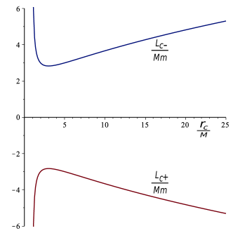
Figure 2: Angular momentum of a neutral test particle in terms of the radius orbit $r_{c}/M$.

As for the energy of circular orbits, we see from Eq.(40) that it does not depend explicitly on the value of the charge, but only on the radial distance from the central punctual mass. This, however, does not mean that the energy does not depend on the charge at all. Indeed, from Eq.(39) we see that, for a given angular momentum, the charge $q$ influences the value of the circular orbit radius which, in turn, enters the expression for the energy. The behavior of the energy in terms of the radial distance is depicted in Fig.3.

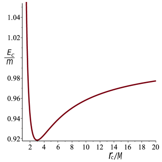
Figure 3: Energy of a charged test particle in terms of the radius orbit $r_{c}/M$.

As the radius approaches the limiting value $r_{c}/M=G/c^{2}=0.774\times 10^{-28}$ cm g^-1, the energy diverges indicating that a test particle cannot be situated on the minimum radius. The energy has an extremal located at the radius $r_{c}/M=3G/c^{2}=2.227\times 10^{-28}$ cm g^-1. We will see below that it corresponds to a particular orbit at which the particle stays at rest. At spatial infinity, we see that $E_{c+}\rightarrow mc^{2}$ which corresponds to the rest energy of the particle outside the influence of the magnetic and gravitational fields.

Let us now consider the conditions under which the particle can remain at rest $(L=0)$ with respect to an observer at infinity. From Eq.(23) for $q\neq 0$ we find the trivial rest radius $r_{r}=0$ for which the energy of the particle is $E_{r}=0$. In addition, the non-trivial solution is given by the rest radii

$$\frac{r_{r\;\pm}}{M}=\frac{c^{2}q^{2}-2\Sigma Gm^{2}\pm\sqrt{c^{2}q^{2}\left(c^{2}q^{2}-8\Sigma Gm^{2}\right)}}{2\Sigma m^{2}c^{2}}.$$ (41)

The behavior of these radii is depicted in Fig. 4. We can see that these solutions are physically realizable in the sense that the radii are always positive for all values of $q/m$ that satisfy the condition $q^{2}\geq 8m^{2}G$. Indeed, the existence of a rest radius is restricted by the discriminant $q^{2}-8m^{2}G$ in Eq.(41). For time-like test particles with $q^{2}/m^{2}>8G$, there exist an inner radius $r_{r-}$ and an outer radius $r_{r+}$ at which the particle can remain at rest. For the limiting value $q^{2}/m^{2}=8G$, the two radii coincide with $r_{r+}=r_{r-}=3GM/c^{2}$. Instead, if $q^{2}/m^{2}<8G$, no radius exists at which the particle could stay at rest. Clearly, the existence of a rest radius is determined by the value of the test particle effective charge, indicating that a zero angular momentum orbit is the consequence of an electromagnetic effect due to the interaction of the test charge and the magnetic background.

For the outer radius $r_{r\,+}$ we have two possible positive values of the corresponding energy, namely,

$$E_{r+}^{(\pm)}=+\frac{mc^{2}\sqrt{2q^{2}\left[q^{2}-2Gm^{2}\pm\sqrt{q^{2}(q^{2}-8Gm^{2})^{2}}\right]^{3}}}{\left[q^{2}\pm\sqrt{q^{2}(q^{2}-8Gm^{2})^{2}}\right]^{2}},$$ (42)

whereas for the inner radius $r_{r\,-}$, the two possible energies are always negative

$$E_{r-}^{(\pm)}=-E_{r+}^{(\pm)}\ .$$ (43)

In Fig. 5, we show the behavior of the energy at the outer rest radius. The minimum value of $\pm(3\sqrt{6}/8)mc^{2}$ is reached for $q^{2}=8Gm^{2}$, i.e., when the inner and outer radii coincide.

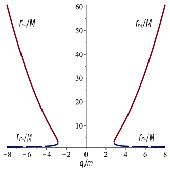
Figure 4: Radii of the time-like orbits characterized by the conditions $L=0$ and $d\Phi/dr=0$ (see Eq.41). In this graphic the radii $r_{r+}/M$ (solid curve) and $r_{r-}/M$ (dashed curve) are plotted as functions of $q/m$.

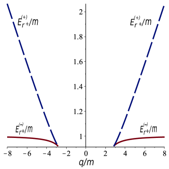
Figure 5: Energy of the charged particles for the time-like orbits characterized by the conditions $L=0$ and $d\Phi/dr=0$ (see Eqs.(42) and (43)). In this graphic the energy $E_{r+}/m$ for the radius $r_{r+}$(solid curve) and $E_{r+}/m$ for the radius $r_{r-}$(dashed curve) are plotted as functions of $q/m$.

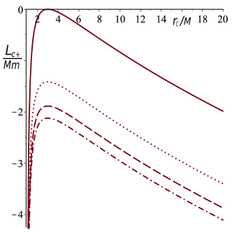
Figure 6: Angular momentum of charged particles in a time-like circular orbit (see Eq. (39)). In this graphic the angular momentum $L_{c}^{+}/Mm$ is plotted as a function of the radius $r_{c}/M$ for some values of $q/m$. The continuous curve corresponds to the value $q/m=2\sqrt{2}$.

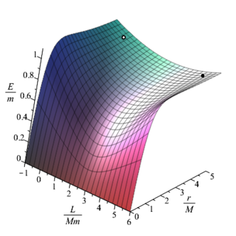
Figure 7: The energy of a particle with charge-to-mass-ratio $q/m=2\sqrt{2}$ is plotted as a function of $r/M$ and the angular momentum $L/Mm$. Time-like circular orbits exist for $r/M>1$. The last stable circular orbit is represented by a black point ($r/M=3,L_{lsco+}=4\sqrt{2}Mm$). The orbit with the same radius ($r/M=3$), but zero angular momentum ($L_{lsco-}=0$) is represented by a white point.

We now investigate the properties of the last stable circular orbit. According to Eq.(29), the angular momentum for this particular orbit must satisfy the relationship

$$L_{lsco\;\pm}=\frac{q\sqrt{G}M}{c}\pm\frac{(c^{2}r+GM)m}{c^{2}}\sqrt{\frac{\Sigma GM(2c^{2}r-GM)}{G^{2}M^{2}-6c^{2}GMr+3c^{4}r^{2}}}.$$ (44)

On the other hand, the angular momentum for any circular orbit is given by Eq.(39). Then, the comparison of Eqs.(44) and (39) yields the condition $r(c^{2}r-3GM)=0$. Therefore, the radius of the last stable circular orbit is given by

$$r_{lsco}=\frac{3GM}{c^{2}}\ ,$$ (45)

which, remarkably, does not depend on the value of the charge $q$. The corresponding angular momentum can be expressed as

$$L_{lsco\;\pm}=\frac{q\sqrt{G}M}{c}\pm\frac{2\sqrt{2\Sigma}GMm}{c^{2}},$$ (46)

and the energy reduces to

$$E_{lsco\;\pm}=\pm\frac{3}{4}\sqrt{\frac{3\Sigma}{2}}mc\ .$$ (47)

As we can see, the angular momentum depends explicitly on the value of the mass $m$ and charge $q$ of the test particle. Additionally, for space-like curves the angular momentum of the last stable circular orbit is not defined, whereas for a null curve it is $L_{lsco\;\pm}={q\sqrt{G}M}/{c}$, and for a time-like particle it is $L_{lsco\;\pm}=(q\sqrt{G}\pm 2\sqrt{2}Gm)M/c$. Accordingly, if the charge of the particle is $q=2\sqrt{2G}m$, then $L_{lsco-}=L_{c+}=L_{r}=0$. Analogously, if $q=-2\sqrt{2G}m$, then $L_{lsco+}=L_{c-}=L_{r}=0$.

Thus, we conclude that the last stable circular orbit occurs at the radius $r=3GM/c^{2}$, independently of the value of the charge. Moreover, on the last stable orbit the particle is at rest, if the value of the charge is $q=\pm 2\sqrt{2G}m$ (see Fig. 6).

In Fig. 7, we present the general behavior of the energy function $E=\pm mc\sqrt{\Phi}$ in terms of the effective potential $\Phi$ given by Eq.(37). The branch corresponding to the positive energy of a particle with charge-to-mass-ratio $q/m=2\sqrt{2G}$ is plotted as a function of $r/M$ and the angular momentum $L/Mm$. We see that the effective potential (energy) tends to a constant at infinity. Since the radius for the last stable circular orbit is $r_{lsco}=3GM/c^{2}$, for a particle with charge $q/m=2\sqrt{2G}$ it is possible to stay at rest with $L_{lsco-}=0$ (white point in Fig.7) or with angular momentum $L_{lsco+}=4\sqrt{2}GMm/c$ (black point in Fig.7). A similar result is obtained if the charge is negative, corresponding to the angular momentum $-4\sqrt{2}G/c$, which indicates rotation in the counterclockwise direction.

It is worth noticing that a neutral particle cannot stay at rest with zero angular momentum. This can be deduced by replacing $q=0$ in Eqs.(41), (42) and (43). In fact, with a zero value of $q$ we obtain a negative rest radius. Finally, from Eqs.(45) and (46) we see that the last time-like stable circular orbit for neutral test particles can be placed at $r=3GM/c^{2}$ with angular momentum $L_{lsco\;\pm}={\pm 2\sqrt{2}GMm}/{c}$. Moreover, a neutral massless test particle can get $L=0$ only at $r=0$, as expected.

We conclude that from an observational point of view the most important characteristic of a conformastatic punctual mass is the radius of the last stable circular orbit $r_{lsco}=3GM/c^{2}$, which does not depend on the value of the test charge $q$. For simplicity, consider the case $q=0$. We should compare this value of $r_{lsco}$ with the corresponding one in the case of axisymmetric fields. The Reissner-Nordström (RN) metric with charge $Q$ would be the obvious candidate to perform the comparison. It is well-known that the magnetic RN metric can easily be obtained by changing $Q^{2}\rightarrow P^{2}$, where $P$ is the magnetic charge, in all the components of the metric. If we then suppose that $P$ is proportional to $M$, we would obtain the corresponding metric for an axisymmetric punctual mass with a magnetic field. In fact, this metric becomes spherically symmetric as a result of the symmetry properties of the field equations. The motion of a neutral test particle in the RN field was investigated in detail in (Pugliese et al., 2011a), where it was shown that $r_{lsco}^{{}_{RN}}\in[3/2,6)GM/c^{2}$ for all the relevant values of $Q/M$. This interval includes the value $3GM/c^{2}$ that corresponds to the conformastatic case. This implies that by only measuring the radius of the last stable circular orbit, it is not possible to differentiate between axial and conformal symmetry. We will therefore consider a different test particle motion in the next section.

V Perihelion advance in a conformastatic magnetized spacetime

One of the most important tests of general relativity and modified theories of gravitation in astrophysical scale is the perihelion advance of celestial objects. In this section, we present the analytic expressions which determine the perihelion advance of charged test particles, moving in a conformastatic spacetime under the presence of a magnetic field. Starting from the first integral (15), we restrict the analysis to the motion of a particle on the plane with $z=0$. Then, we have

$$\Bigg{(}\frac{dr}{d\varphi}\Bigg{)}^{2}=-r^{2}\Bigg{[}1+\frac{m^{2}r^{2}}{\big{(}L-\frac{q}{c}A_{\varphi}\big{)}^{2}}\Bigg{(}\Sigma(1-U)^{2}-\frac{E^{2}}{m^{2}c^{2}}(1-U)^{4}\Bigg{)}\Bigg{]},$$ (48)

where all the quantities are evaluated at $z=0$ and we have used the expressions for the energy and angular momentum of the particle given by Eqs.(13) and (14), respectively. This expression for the perihelion advance is valid for any harmonic function $U=U(r,z=0)$.

To evaluate the perihelion advance in a concrete example, we consider the punctual solution with $U=\frac{GM}{c^{2}r}$ for a neutral test particle ($q=0)$. Then, introducing the auxiliary function $v=1+\frac{GM}{c^{2}r}$, Eq.(48) reduces to

$$\left(\frac{dv}{d\varphi}\right)^{2}+(v-1)^{2}=-\frac{G^{2}m^{2}M^{2}}{c^{4}L^{2}}\left(c^{2}v^{2}-\frac{E^{2}}{m^{2}c^{2}}v^{4}\right)\ .$$ (49)

Calculating the derivative of the above equation, we obtain

$$\frac{d^{2}v}{d\varphi^{2}}+(1+\alpha^{2})v=1+2\beta^{2}v^{3}\ ,\quad\alpha=\frac{GmM}{cL}\ ,\quad\beta=\frac{GME}{c^{3}L}\ .$$ (50)

The analytic solution to this equation can be found by using standard methods of ordinary differential equations. However, it is enough to consider an approximate solution of the form

$$v=v_{c}(1+\omega)\ ,$$ (51)

where $v_{c}=1+\frac{GM}{c^{2}r_{c}}$ is the solution for a circular orbit with radius $r_{c}$. Then, from Eq.(50) we obtain

$$v_{c}\frac{d^{2}\omega}{d\varphi^{2}}+(1+\alpha^{2}-6\beta^{2})v_{c}\omega+(1+\alpha^{2}-2\beta^{2})v_{c}=1\ ,$$ (52)

where we have considered only linear terms in $\omega$. In the limiting case of a circular orbit ($\omega=0)$, the condition $1+\alpha^{2}-2\beta^{2}=\frac{1}{v_{c}}\sim 1-\frac{GM}{c^{2}r_{c}}$ must hold and, consequently, Eq(52) reduces to

$$\frac{d^{2}\omega}{d\varphi^{2}}+\left(1-\frac{GM}{c^{2}r_{c}}-4\beta^{2}\right)\omega=0\ ,$$ (53)

whose solution can be written as

$$\omega=\omega_{0}\cos\left[\left(1-\frac{GM}{c^{2}r_{c}}-4\beta^{2}\right)\varphi\right]\ .$$ (54)

The perihelion shift can be calculated at the maximum value of the solution, i.e., when $\left(1-\frac{GM}{c^{2}r_{c}}-4\beta^{2}\right)\varphi=2\pi$, which can be written as $\phi=2\pi+\Delta\varphi$, with $\Delta\varphi=\pi\left(\frac{GM}{c^{2}r_{c}}+4\beta^{2}\right)$. A straightforward computation by using Eqs.(50), (39) and (40), to the first order in $1/r_{c}$, leads to

$$\Delta\varphi=\frac{5\pi GM}{c^{2}r_{c}}\ .$$ (55)

This is the final value of the perihelion advance for a neutral test mass in the gravitational field of a punctual mass, endowed with a magnetic field. This compares with the value obtained for the Schwarzschild spacetime $\Delta\varphi=\frac{6\pi GM}{c^{2}r_{c}}$. The perihelion advance around a punctual magnetic mass is therefore always smaller than the value obtained in Einstein gravity alone. We conclude that the perihelion advance permits us to differentiate between a spherically symmetric mass and a conformally symetric punctual magnetic mass.

VI Conclusions

In this work, we have shortly shown the characteristics of the motion of a charged particle along circular orbits in a spacetime described by a conformastatic solution of the Einstein-Maxwell equations, which is also a solution of the general axisymmetric static electrovacuum Weyl class.

As a particular example we have considered the case of a charged particle moving in the gravitational field of a punctual source placed at the origin of coordinates. Our analysis is based on the study of the behavior of an effective potential that determines the position and stability properties of circular orbits. We have found that a classical radius $r=3GM/c^{2}$ of circular orbits exists with zero angular momentum. This phenomenon is interpreted as a consequence of the repulsive electric force that exists between the charge distribution and the charged test particle. Interestingly, we have found this effect in a singularity-free spacetime, implying that it is not exclusive to the case of naked singularities. Indeed, other configurations show a similar behavior even in the case of non-test particles; for instance, the the Majumdar-Papapetrou system (Majumdar, 1947; Papapetrou, 1945), which is the subset of the Einstein-Maxwell-charged dust matter theory with the peculiar characteristic that the charge of each particle is equal to its mass.

Moreover, we have obtained a region of stability determined by the angular momentum $L_{lsco}^{\pm}/Mm=q\sqrt{G}/(mc)+2\sqrt{2}G/c$ and the radius $r=3GM/c^{2}$. It is worth noticing that a neutral particle can not be located at rest with angular momentum zero. We also notice that the last time-like stable circular orbit for neutral test particles with $m\neq 0$ can be placed at $r=3GM/c^{2}$ with angular momentum $L_{lsco\;\pm}={\pm 2\sqrt{2}GMm}/{c}$, and that neutral massless particles can get $L=0$ only when they are placed at $r=0$, as expected.

In addition, we have also calculated an expression for the perihelion advance of a test particle in a general magnetized conformastatic spacetime. In the particular case of a punctual magnetic mass, we found the explicit value of the perihelion advance, which turns out to be $5/6$ of the Schwarzschild value.

Our results can be used to test the possibility that conformally symetric mass distributions exist in Nature. Suppose that some observations show that the radius of the last stable circular orbit around a static compact object of mass $M$ is $r_{lsco}={3GM/c^{2}}$. Since this value is predicted for the punctual magnetic mass as well as for a Reissner-Nordström source, it is not possible to determine the symmetry of the source. Nevertheless, if observations show that the perihelion shift around a compact object is $\Delta\varphi=\frac{5\pi GM}{c^{2}r_{c}}$, then the compact object could be identified as a conformally symmetric punctual magnetic mass.

References

- González et al. (2008) G. A. González, A. C. Gutiérrez-Piñeres, and P. A. Ospina, Physical Review D 78, 064058 (2008).
- Bally and Harrison (1978) J. Bally and E. Harrison, The Astrophysical Journal 220, 743 (1978).
- Uyaniker et al. (2004) B. Uyaniker, W. Reich, and R. Wielebinski, in The Magnetized Interstellar Medium (2004).
- Zamaninasab et al. (2014) M. Zamaninasab, E. Clausen-Brown, T. Savolainen, and A. Tchekhovskoy, Nature 510, 126 (2014).
- Han (2012) J. Han, Proceedings of the International Astronomical Union 8, 213 (2012).
- Gutiérrez-Piñeres (2015) A. C. Gutiérrez-Piñeres, General Relativity and Gravitation 47, 54 (2015), 10.1007/s10714-015-1898-0.
- Guti rrez-Pi eres and Capistrano (2015) A. C. Gutiérrez-Piñeres and A. J. S. Capistrano, Adv. Math. Phys. 2015, 916026 (2015), arXiv:1504.01138 [gr-qc] .
- Gutiérrez-Piñeres et al. (2015) A. C. Gutiérrez-Piñeres, C. S. Lopez-Monsalvo, and H. Quevedo, General Relativity and Gravitation 47, 1 (2015).
- Synge (1960) J. Synge, Relativity: the general theory (North-Holland Pub. Co.; Interscience Publishers, Amsterdam; New York, 1960).
- Gutiérrez-Piñeres and Capistrano (2015) A. C. Gutiérrez-Piñeres and A. J. Capistrano, arXiv preprint arXiv:1510.05400 (2015).
- Pugliese et al. (2011a) D. Pugliese, H. Quevedo, and R. Ruffini, Phys. Rev. D 83, 104052 (2011a).
- Pugliese et al. (2011b) D. Pugliese, H. Quevedo, and R. Ruffini, Phys. Rev. D 83, 024021 (2011b).
- Gutiérrez-Piñeres et al. (2013) A. C. Gutiérrez-Piñeres, G. A. González, and H. Quevedo, Phys. Rev. D 87, 044010 (2013).
- Stephani et al. (2009) H. Stephani, D. Kramer, M. MacCallum, C. Hoenselaers, and E. Herlt, Exact solutions of Einstein’s field equations (Cambridge University Press, 2009).
- Majumdar (1947) S. D. Majumdar, Physical Review 72, 390 (1947).
- Papapetrou (1945) A. Papapetrou, in Proceedings of the Royal Irish Academy. Section A: Mathematical and Physical Sciences, Vol. 51 (JSTOR, 1945) pp. 191–204.