Learning Preferences for Manipulation Tasks
from Online Coactive Feedback

Abstract

We consider the problem of learning preferences over trajectories for mobile manipulators such as personal robots and assembly line robots. The preferences we learn are more intricate than simple geometric constraints on trajectories; they are rather governed by the surrounding context of various objects and human interactions in the environment. We propose a coactive online learning framework for teaching preferences in contextually rich environments. The key novelty of our approach lies in the type of feedback expected from the user: the human user does not need to demonstrate optimal trajectories as training data, but merely needs to iteratively provide trajectories that slightly improve over the trajectory currently proposed by the system. We argue that this coactive preference feedback can be more easily elicited than demonstrations of optimal trajectories. Nevertheless, theoretical regret bounds of our algorithm match the asymptotic rates of optimal trajectory algorithms.

We implement our algorithm on two high degree-of-freedom robots, PR2 and Baxter, and present three intuitive mechanisms for providing such incremental feedback. In our experimental evaluation we consider two context rich settings – household chores and grocery store checkout – and show that users are able to train the robot with just a few feedbacks (taking only a few minutes).

I Introduction

Recent advances in robotics have resulted in mobile manipulators with high degree of freedom (DoF) arms. However, the use of high DoF arms has so far been largely successful only in structured environments such as manufacturing scenarios, where they perform repetitive motions (e.g., recent deployment of Baxter on assembly lines). One challenge in the deployment of these robots in unstructured environments (such as a grocery checkout counter or at our homes) is their lack of understanding of user preferences and thereby not producing desirable motions. In this work we address the problem of learning preferences over trajectories for high DoF robots such as Baxter or PR2. We consider a variety of household chores for PR2 and grocery checkout tasks for Baxter.

A key problem for high DoF manipulators lies in identifying an appropriate trajectory for a task. An appropriate trajectory not only needs to be valid from a geometric point (i.e., feasible and obstacle-free, the criteria that most path planners focus on), but it also needs to satisfy the user’s preferences. Such users’ preferences over trajectories can be common across users or they may vary between users, between tasks, and between the environments the trajectory is performed in. For example, a household robot should move a glass of water in an upright position without jerks while maintaining a safe distance from nearby electronic devices. In another example, a robot checking out a knife at a grocery store should strictly move it at a safe distance from nearby humans. Furthermore, straight-line trajectories in Euclidean space may no longer be the preferred ones. For example, trajectories of heavy items should not pass over fragile items but rather move around them. These preferences are often hard to describe and anticipate without knowing where and how the robot is deployed. This makes it infeasible to manually encode them in existing path planners (e.g., Zucker et al. [63], Sucan et al. [57], Schulman et al. [50]) a priori.

In this work we propose an algorithm for learning user preferences over trajectories through interactive feedback from the user in a coactive learning setting [51]. In this setting the robot learns through iterations of user feedback. At each iteration robot receives a task and it predicts a trajectory. The user responds by slightly improving the trajectory but not necessarily revealing the optimal trajectory. The robot use this feedback from user to improve its predictions for future iterations. Unlike in other learning settings, where a human first demonstrates optimal trajectories for a task to the robot [4], our learning model does not rely on the user’s ability to demonstrate optimal trajectories a priori. Instead, our learning algorithm explicitly guides the learning process and merely requires the user to incrementally improve the robot’s trajectories, thereby learning preferences of user and not the expert. From these interactive improvements the robot learns a general model of the user’s preferences in an online fashion. We realize this learning algorithm on PR2 and Baxter robots, and also leverage robot-specific design to allow users to easily give preference feedback.

Our experiments show that a robot trained using this approach can autonomously perform new tasks and if need be, only a small number of interactions are sufficient to tune the robot to the new task. Since the user does not have to demonstrate a (near) optimal trajectory to the robot, the feedback is easier to provide and more widely applicable. Nevertheless, it leads to an online learning algorithm with provable regret bounds that decay at the same rate as for optimal demonstration algorithms (eg. Ratliff et al. [45]).

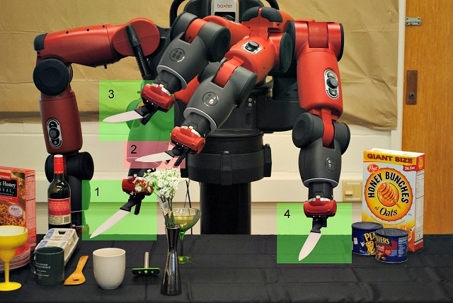
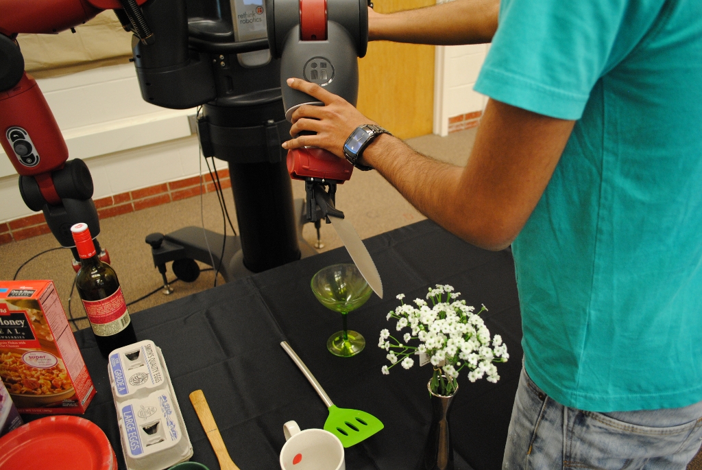
Figure 1: Zero-G feedback: Learning trajectory preferences from suboptimal zero-G feedback. (Left) Robot plans a bad trajectory (waypoints 1-2-4) with knife close to flower. As feedback, user corrects waypoint 2 and moves it to waypoint 3. (Right) User providing zero-G feedback on waypoint 2.

In our empirical evaluation we learn preferences for two high DoF robots, PR2 and Baxter, on a variety of household and grocery checkout tasks respectively. We design expressive trajectory features and show how our algorithm learns preferences from online user feedback on a broad range of tasks for which object properties are of particular importance (e.g., manipulating sharp objects with humans in the vicinity). We extensively evaluate our approach on a set of 35 household and 16 grocery checkout tasks, both in batch experiments as well as through robotic experiments wherein users provide their preferences to the robot. Our results show that our system not only quickly learns good trajectories on individual tasks, but also generalizes well to tasks that the algorithm has not seen before. In summary, our key contributions are:

1. We present an approach for teaching robots which does not rely on experts’ demonstrations but nevertheless gives strong theoretical guarantees.

2. We design a robotic system with multiple easy to elicit feedback mechanisms to improve the current trajectory.

3. We implement our algorithm on two robotic platforms, PR2 and Baxter, and support it with a user study.

4. We consider preferences that go beyond simple geometric criteria to capture object and human interactions.

5. We design expressive trajectory features to capture contextual information. These features might also find use in other robotic applications.

In the following section we discuss related works. In section III we describe our system and feedback mechanisms. Our learning algorithm and trajectory features are discussed in sections IV and IV, respectively. Section VI gives our experiments and results. We discuss future research directions and conclude in section VII.

II Related Work

Path planning is one of the key problems in robotics. Here, the objective is to find a collision free path from a start to goal location. Over the last decade many planning algorithms have been proposed, such as sampling based planners by Lavalle and Kuffner [33], and Karaman and Frazzoli [26], search based planners by Cohen et al. [10], trajectory optimizers by Schulman et al. [50], and Zucker et al. [63] and many more [27]. However, given the large space of possible trajectories in most robotic applications simply a collision free trajectory might not suffice, instead the trajectory should satisfy certain constraints and obey the end user preferences. Such preferences are often encoded as a cost which planners optimize [26, 50, 63]. We address the problem of learning a cost over trajectories for context-rich environments, and from sub-optimal feedback elicited from non-expert users. We now describe related work in various aspects of this problem.

Learning from Demonstration (LfD): Teaching a robot to produce desired motions has been a long standing goal and several approaches have been studied. In LfD an expert provides demonstrations of optimal trajectories and the robot tries to mimic the expert. Examples of LfD includes, autonomous helicopter flights [1], ball-in-a-cup game [30], planning 2-D paths [43, 44], etc. Such settings assume that kinesthetic demonstrations are intuitive to an end-user and it is clear to an expert what constitutes a good trajectory. In many scenarios, especially involving high DoF manipulators, this is extremely challenging to do [2]. This is because the users have to give not only the end-effector’s location at each time-step, but also the full configuration of the arm in a spatially and temporally consistent manner. In Ratliff et al. [45] the robot observes optimal user feedback but performs approximate inference. On the other hand, in our setting, the user never discloses the optimal trajectory or feedback, but instead, the robot learns preferences from sub-optimal suggestions for how the trajectory can be improved.
 
  Noisy demonstrations and other forms of user feedback: Some later works in LfD provided ways for handling noisy demonstrations, under the assumption that demonstrations are either near optimal, as in Ziebart et al. [62], or locally optimal, as in Levine et al. [36]. Providing noisy demonstrations is different from providing relative preferences, which are biased and can be far from optimal. We compare with an algorithm for noisy LfD learning in our experiments. Wilson et al. [60] proposed a Bayesian framework for learning rewards of a Markov decision process via trajectory preference queries. Our approach advances over [60] and Calinon et. al. [9] in that we model user as a utility maximizing agent. Further, our score function theoretically converges to user’s hidden function despite recieving sub-optimal feedback.

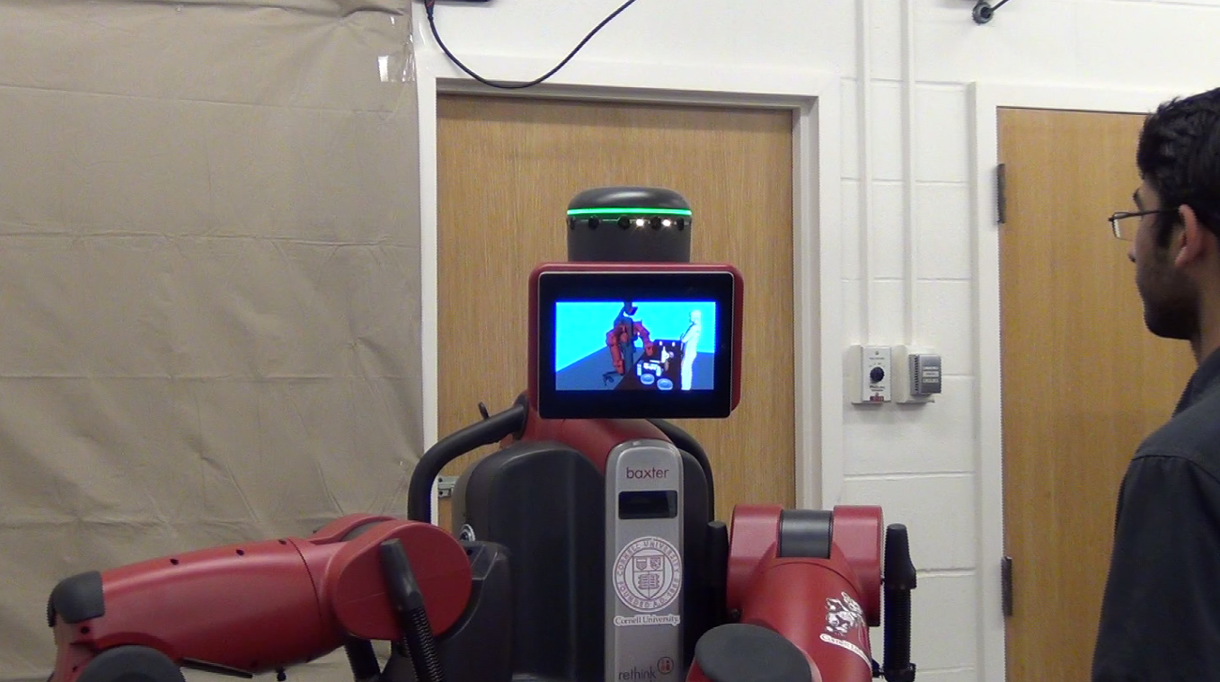
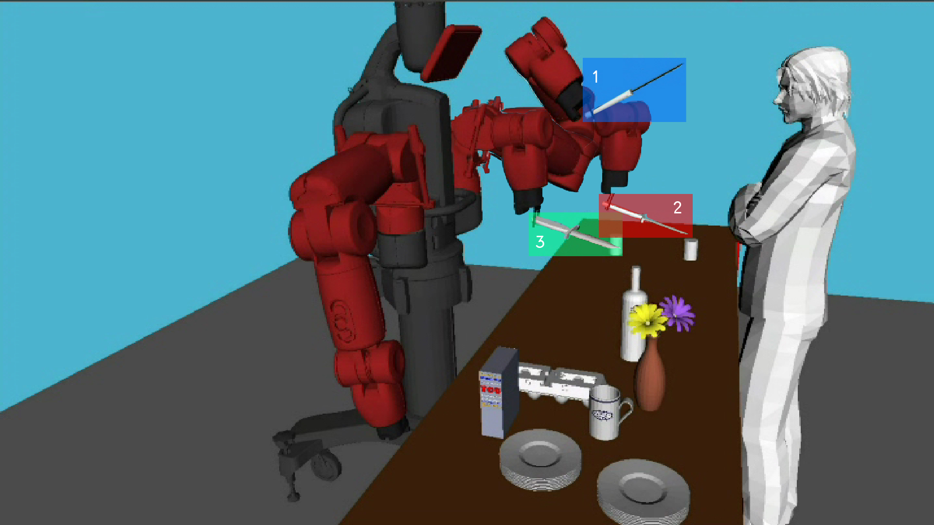
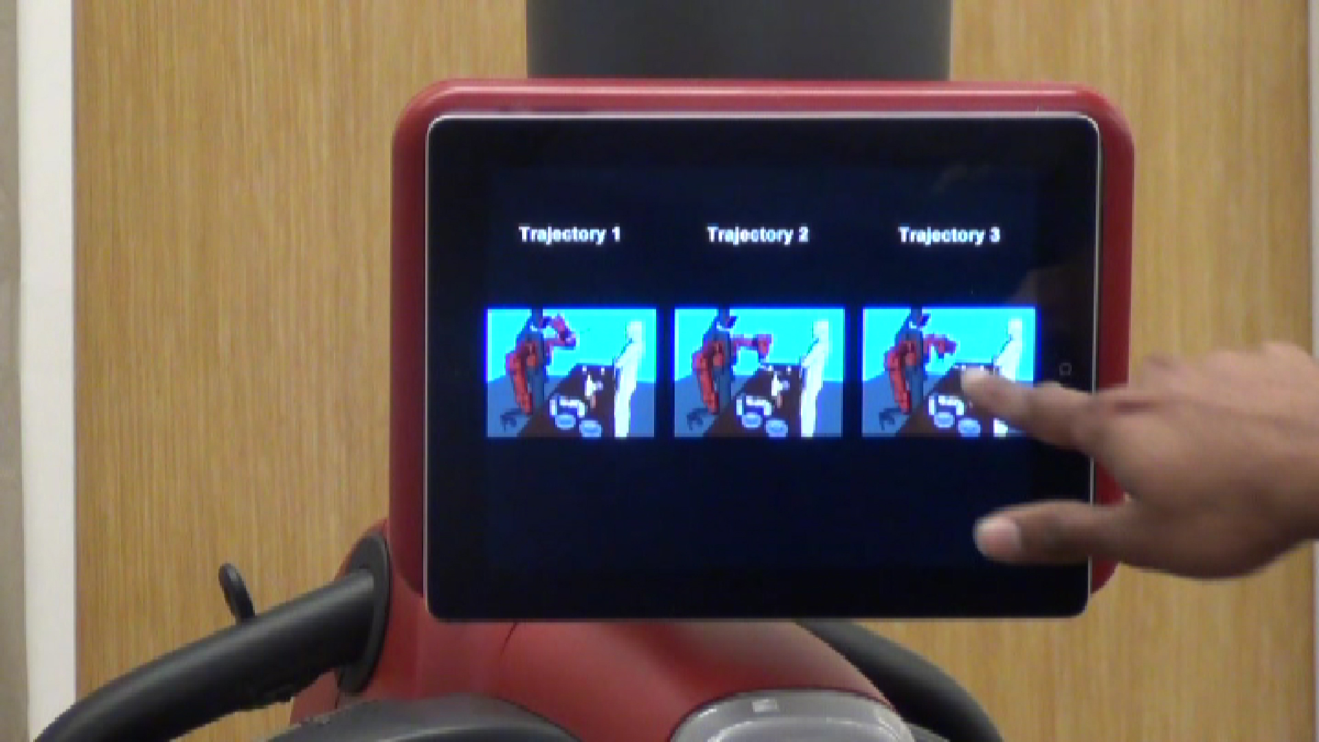
Figure 2: Re-rank feedback mechanism: (Left) Robot ranks trajectories using the score function and (Middle) displays top three trajectories on a touch screen device (iPad here). (Right) As feedback, the user improves the ranking by selecting the third trajectory.

In the past, various interactive methods (e.g. human gestures) [8, 56] have been employed to teach assembly line robots. However, these methods required the user to interactively show the complete sequence of actions, which the robot then remembered for future use. Recent works by Nikolaidis et al. [39, 40] in human-robot collaboration learns human preferences over a sequence of sub-tasks in assembly line manufacturing. However, these works are agnostic to the user preferences over robot’s trajectories. Our work could complement theirs to achieve better human-robot collaboration.
 
  Learning preferences over trajectories: User preferences over robot’s trajectories have been studied in human-robot interaction. Sisbot et. al. [55, 54] and Mainprice et. al. [37] planned trajectories satisfying user specified preferences in form of constraints on the distance of the robot from the user, the visibility of the robot and the user’s arm comfort. Dragan et. al. [14] used functional gradients [47] to optimize for legibility of robot trajectories. We differ from these in that we take a data driven approach and learn score functions reflecting user preferences from sub-optimal feedback.
 
  Planning from a cost function: In many applications, the goal is to find a trajectory that optimizes a cost function. Several works build upon the sampling-based planner RRT [33] to optimize various cost heuristics [17, 11, 20]. Additive cost functions with Lipschitz continuity can be optimized using optimal planners such as RRT* [26]. Some approaches introduce sampling bias [35] to guide the sampling based planner. Recent trajectory optimizers such as CHOMP [47] and TrajOpt [50] provide optimization based approaches to finding optimal trajectory. Our work is complementary to these in that we learn a cost function while the above approaches optimize a cost.

Our work is also complementary to few works in path planning. Berenson et al. [5] and Phillips et al. [41] consider the problem of trajectories for high-dimensional manipulators. For computational reasons they create a database of prior trajectories, which we could leverage to train our system. Other recent works consider generating human-like trajectories [15, 14, 58]. Humans-robot interaction is an important aspect and our approach could incorporate similar ideas.
 
  Application domain: In addition to above mentioned differences we also differ in the applications we address. We capture the necessary contextual information for household and grocery store robots, while such context is absent in previous works. Our application scenario of learning trajectories for high DoF manipulations performing tasks in presence of different objects and environmental constraints goes beyond the application scenarios that previous works have considered. Some works in mobile robotics learn context-rich perception-driven cost functions, such as Silver et al. [53], Kretzschmar et al. [32] and Kitani et al. [28]. In this work we use features that consider robot configurations, object-object relations, and temporal behavior, and use them to learn a score function representing the preferences over trajectories.

III Coactive learning with incremental feedback

We first give an overview of our robot learning setup and then describe in detail three mechanisms of user feedback.

III-A Robot learning setup

We propose an online algorithm for learning preferences in trajectories from sub-optimal user feedback. At each step the robot receives a task as input and outputs a trajectory that maximizes its current estimate of some score function. It then observes user feedback – an improved trajectory – and updates the score function to better match the user preferences. This procedure of learning via iterative improvement is known as coactive learning. We implement the algorithm on PR2 and Baxter robots, both having two 7 DoF arms. In the process of training, the initial trajectory proposed by the robot can be far-off the desired behavior. Therefore, instead of directly executing trajectories in human environments, users first visualize them in the OpenRAVE simulator [13] and then decide the kind of feedback they would like to provide.

III-B Feedback mechanisms

Our goal is to learn even from feedback given by non-expert users. We therefore require the feedback only to be incrementally better (as compared to being close to optimal) in expectation, and will show that such feedback is sufficient for the algorithm’s convergence. This stands in contrast to learning from demonstration (LfD) methods [1, 30, 43, 44] which require (near) optimal demonstrations of the complete trajectory. Such demonstrations can be extremely challenging and non-intuitive to provide for many high DoF manipulators [2]. Instead, we found [21, 22] that it is more intuitive for users to give incremental feedback on high DoF arms by improving upon a proposed trajectory. We now summarize three feedback mechanisms that enable the user to iteratively provide improved trajectories.
 
  (a) Re-ranking: We display the ranking of trajectories using OpenRAVE [13] on a touch screen device and ask the user to identify whether any of the lower-ranked trajectories is better than the top-ranked one. The user sequentially observes the trajectories in order of their current predicted scores and clicks on the first trajectory which is better than the top ranked trajectory. Figure 2 shows three trajectories for moving a knife. As feedback, the user moves the trajectory at rank 3 to the top position. Likewise, Figure 3 shows three trajectories for moving an egg carton. Using the current estimate of score function robot ranks them as red ($1^{st}$), green ($2^{nd}$) and blue ($3^{rd}$). Since eggs are fragile the user selects the green trajectory.
 

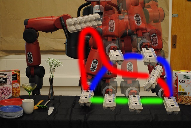
Figure 3: Re-ranking feedback: Shows three trajectories for moving egg carton from left to right. Using the current estimate of score function robot ranks them as red, green and blue. As feedback user clicks the green trajectory. Preference: Eggs are fragile. They should be kept upright and near the supporting surface.

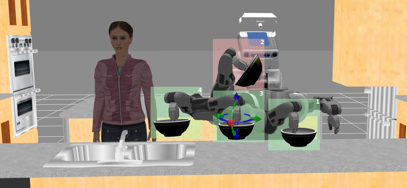
Figure 4: Interactive feedback. Task here is to move a bowl filled with water. The robot presents a bad trajectory with waypoints 1-2-4 to the user. As feedback user moves waypoint 2 (red) to waypoint 3 (green) using Rviz interactive markers. The interactive markers guides the user to correct the waypoint.

(b) Zero-G: This is a kinesthetic feedback. It allows the user to correct trajectory waypoints by physically changing the robot’s arm configuration as shown in Figure 1. High DoF arms such as the Barrett WAM and Baxter have zero-force gravity-compensation (zero-G) mode, under which the robot’s arms become light and the users can effortlessly steer them to a desired configuration. On Baxter, this zero-G mode is automatically activated when a user holds the robot’s wrist (see Figure 1, right). We use this zero-G mode as a feedback method for incrementally improving the trajectory by correcting a waypoint. This feedback is useful (i) for bootstrapping the robot, (ii) for avoiding local maxima where the top trajectories in the ranked list are all bad but ordered correctly, and (iii) when the user is satisfied with the top ranked trajectory except for minor errors.
 
  (c) Interactive: For the robots whose hardware does not permit zero-G feedback, such as PR2, we built an alternative interactive Rviz-ROS [18] interface for allowing the users to improve the trajectories by waypoint correction. Figure 4 shows a robot moving a bowl with one bad waypoint (in red), and the user provides a feedback by correcting it. This feedback serves the same purpose as zero-G.
 
  Note that, in all three kinds of feedback the user never reveals the optimal trajectory to the algorithm, but only provides a slightly improved trajectory (in expectation).

IV Learning and Feedback Model

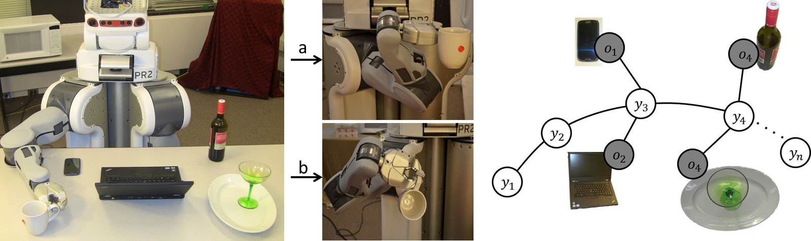
Figure 5: (Left) An environment with a few objects where the robot was asked to move the cup on the left to the right. (Middle) There are two ways of moving it, ‘a’ and ‘b’, both are suboptimal in that the arm is contorted in ‘a’ but it tilts the cup in ‘b’. Given such constrained scenarios, we need to reason about such subtle preferences. (Right) We encode preferences concerned with object-object interactions in a score function expressed over a graph. Here $y_{1},\ldots,y_{n}$ are different waypoints in a trajectory. The shaded nodes corresponds to environment (table node not shown here). Edges denotes interaction between nodes.

We model the learning problem in the following way. For a given task, the robot is given a context $x$ that describes the environment, the objects, and any other input relevant to the problem. The robot has to figure out what is a good trajectory $y$ for this context. Formally, we assume that the user has a scoring function $s^{*}(x,y)$ that reflects how much he values each trajectory $y$ for context $x$. The higher the score, the better the trajectory. Note that this scoring function cannot be observed directly, nor do we assume that the user can actually provide cardinal valuations according to this function. Instead, we merely assume that the user can provide us with preferences that reflect this scoring function. The robot’s goal is to learn a function $s(x,y;w)$ (where $w$ are the parameters to be learned) that approximates the user’s true scoring function $s^{*}(x,y)$ as closely as possible.
 
  Interaction Model. The learning process proceeds through the following repeated cycle of interactions.

• Step 1: The robot receives a context $x$ and uses a planner to sample a set of trajectories, and ranks them according to its current approximate scoring function $s(x,y;w)$.

• Step 2: The user either lets the robot execute the top-ranked trajectory, or corrects the robot by providing an improved trajectory $\bar{y}$. This provides feedback indicating that $s^{*}(x,\bar{y})>s^{*}(x,y)$.

• Step 3: The robot now updates the parameter $w$ of $s(x,y;w)$ based on this preference feedback and returns to step 1.

Regret. The robot’s performance will be measured in terms of regret, $REG_{T}=\frac{1}{T}\sum_{t=1}^{T}[s^{*}(x_{t},{y}^{*}_{t})-s^{*}(x_{t},{y}_{t})]$, which compares the robot’s trajectory ${y}_{t}$ at each time step $t$ against the optimal trajectory ${y}_{t}^{*}$ maximizing the user’s unknown scoring function $s^{*}(x,{y})$, ${y}_{t}^{*}=argmax_{y}s^{*}(x_{t},{y})$. Note that the regret is expressed in terms of the user’s true scoring function $s^{*}$, even though this function is never observed. Regret characterizes the performance of the robot over its whole lifetime, therefore reflecting how well it performs throughout the learning process. We will employ learning algorithms with theoretical bounds on the regret for scoring functions that are linear in their parameters, making only minimal assumptions about the difference in score between $s^{*}(x,\bar{y})$ and $s^{*}(x,y)$ in Step 2 of the learning process.
  Expert Vs Non-expert user. We refer to an expert user as someone who can demonstrate the optimal trajectory $y^{*}$ to the robot. For example, robotics experts such as, the pilot demonstrating helicopter maneuver in Abbeel et al. [1]. On the other hand, our non-expert users never demonstrate $y^{*}$. They can only provide feedback $\bar{y}$ indicating $s^{*}(x,\bar{y})>s^{*}(x,y)$. For example, users working with assistive robots on assembly lines.

V Learning Algorithm

For each task, we model the user’s scoring function $s^{*}(x,y)$ with the following parametrized family of functions.

$$s(x,y;w)=w\cdot\phi(x,y)$$ (1)

$w$ is a weight vector that needs to be learned, and $\phi(\cdot)$ are features describing trajectory $y$ for context $x$. Such linear representation of score functions have been previously used for generating desired robot behaviors [1, 44, 62].

We further decompose the score function in two parts, one only concerned with the objects the trajectory is interacting with, and the other with the object being manipulated and the environment

$$s(x,y;w_{O},w_{E}) =s_{O}(x,y;w_{O})+s_{E}(x,y;w_{E})$$

$$=w_{O}\cdot\phi_{O}(x,y)+w_{E}\cdot\phi_{E}(x,y)$$ (2)

We now describe the features for the two terms, $\phi_{O}(\cdot)$ and $\phi_{E}(\cdot)$ in the following.

V-A Features Describing Object-Object Interactions

This feature captures the interaction between objects in the environment with the object being manipulated. We enumerate waypoints of trajectory $y$ as $y_{1},..,y_{N}$ and objects in the environment as $\mathcal{O}=\{o_{1},..,o_{K}\}$. The robot manipulates the object $\bar{o}\in\mathcal{O}$. A few of the trajectory waypoints would be affected by the other objects in the environment. For example in Figure 5, $o_{1}$ and $o_{2}$ affect the waypoint $y_{3}$ because of proximity. Specifically, we connect an object $o_{k}$ to a trajectory waypoint if the minimum distance to collision is less than a threshold or if $o_{k}$ lies below $\bar{o}$. The edge connecting $y_{j}$ and $o_{k}$ is denoted as $(y_{j},o_{k})\in\mathcal{E}$.

Since it is the attributes [31] of the object that really matter in determining the trajectory quality, we represent each object with its attributes. Specifically, for every object $o_{k}$, we consider a vector of $M$ binary variables [$l_{k}^{1},..,l_{k}^{M}$], with each $l_{k}^{m}=\{0,1\}$ indicating whether object $o_{k}$ possesses property $m$ or not. For example, if the set of possible properties are {heavy, fragile, sharp, hot, liquid, electronic}, then a laptop and a glass table can have labels [$0,1,0,0,0,1$] and [$0,1,0,0,0,0$] respectively. The binary variables $l_{k}^{p}$ and $l^{q}$ indicates whether $o_{k}$ and $\bar{o}$ possess property $p$ and $q$ respectively. Then, for every ($y_{j},o_{k}$) edge, we extract following four features $\phi_{oo}(y_{j},o_{k})$: projection of minimum distance to collision along x, y and z (vertical) axis and a binary variable, that is 1, if $o_{k}$ lies vertically below $\bar{o}$, 0 otherwise.

We now define the score $s_{O}(\cdot)$ over this graph as follows:

$$s_{O}(x,y;w_{O})=\sum_{(y_{j},o_{k})\in\mathcal{E}}\sum_{p,q=1}^{M}l_{k}^{p}l^{q}[w_{pq}\cdot\phi_{oo}(y_{j},o_{k})]$$ (3)

Here, the weight vector $w_{pq}$ captures interaction between objects with properties $p$ and $q$. We obtain $w_{O}$ in eq. (V) by concatenating vectors $w_{pq}$. More formally, if the vector at position $i$ of $w_{O}$ is $w_{uv}$ then the vector corresponding to position $i$ of $\phi_{O}(x,y)$ will be $\sum_{(y_{j},o_{k})\in\mathcal{E}}l_{k}^{u}l^{v}[\phi_{oo}(y_{j},o_{k})]$.

V-B Trajectory Features

We now describe features, $\phi_{E}(x,y)$, obtained by performing operations on a set of waypoints. They comprise the following three types of the features:

V-B1 Robot Arm Configurations

While a robot can reach the same operational space configuration for its wrist with different configurations of the arm, not all of them are preferred [61]. For example, the contorted way of holding the cup shown in Figure 5 may be fine at that time instant, but would present problems if our goal is to perform an activity with it, e.g. doing the pouring activity. Furthermore, humans like to anticipate robots move and to gain users’ confidence, robot should produce predictable and legible robotic motions [14].

We compute features capturing robot’s arm configuration using the location of its elbow and wrist, w.r.t. to its shoulder, in cylindrical coordinate system, $(r,\theta,z)$. We divide a trajectory into three parts in time and compute 9 features for each of the parts. These features encode the maximum and minimum $r$, $\theta$ and $z$ values for wrist and elbow in that part of the trajectory, giving us 6 features. Since at the limits of the manipulator configuration, joint locks may happen, therefore we also add 3 features for the location of robot’s elbow whenever the end-effector attains its maximum $r$, $\theta$ and $z$ values respectively. Thus obtaining $\phi_{robot}(\cdot)\in\mathbb{R}^{9}$ (3+3+3=9) features for each one-third part and $\phi_{robot}(\cdot)\in\mathbb{R}^{27}$ for the complete trajectory.

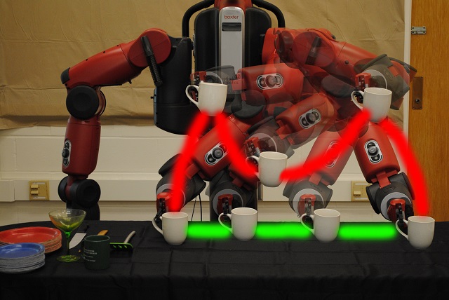
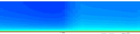
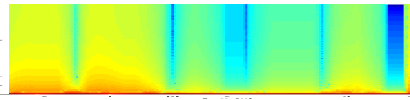
Figure 6: (Top) A good and bad trajectory for moving a mug. The bad trajectory undergoes ups-and-downs. (Bottom) Spectrograms for movement in z-direction: (Left) Good trajectory, (Right) Bad trajectory.

V-B2 Orientation and Temporal Behaviour of the Object to be Manipulated

Object orientation during the trajectory is crucial in deciding its quality. For some tasks, the orientation must be strictly maintained (e.g., moving a cup full of coffee); and for some others, it may be necessary to change it in a particular fashion (e.g., pouring activity). Different parts of the trajectory may have different requirements over time. For example, in the placing task, we may need to bring the object closer to obstacles and be more careful.

We therefore divide trajectory into three parts in time. For each part we store the cosine of the object’s maximum deviation, along the vertical axis, from its final orientation at the goal location. To capture object’s oscillation along trajectory, we obtain a spectrogram for each one-third part for the movement of the object in $x$, $y$, $z$ directions as well as for the deviation along vertical axis (e.g. Figure 6). We then compute the average power spectral density in the low and high frequency part as eight additional features for each. This gives us 9 (=1+4*2) features for each one-third part. Together with one additional feature of object’s maximum deviation along the whole trajectory, we get $\phi_{obj}(\cdot)\in\mathbb{R}^{28}$ (=9*3+1).

V-B3 Object-Environment Interactions

This feature captures temporal variation of vertical and horizontal distances of the object $\bar{o}$ from its surrounding surfaces. In detail, we divide the trajectory into three equal parts, and for each part we compute object’s: (i) minimum vertical distance from the nearest surface below it. (ii) minimum horizontal distance from the surrounding surfaces; and (iii) minimum distance from the table, on which the task is being performed, and (iv) minimum distance from the goal location. We also take an average, over all the waypoints, of the horizontal and vertical distances between the object and the nearest surfaces around it. To capture temporal variation of object’s distance from its surrounding we plot a time-frequency spectrogram of the object’s vertical distance from the nearest surface below it, from which we extract six features by dividing it into grids. This feature is expressive enough to differentiate whether an object just grazes over table’s edge (steep change in vertical distance) versus, it first goes up and over the table and then moves down (relatively smoother change). Thus, the features obtained from object-environment interaction are $\phi_{obj-env}(\cdot)\in\mathbb{R}^{20}$ (3*4+2+6=20).

Final feature vector is obtained by concatenating $\phi_{obj-env}$, $\phi_{obj}$ and $\phi_{robot}$, giving us $\phi_{E}(\cdot)\in\mathbb{R}^{75}$.

Figure 7: Shows our system design, for grocery store settings, which provides users with three choices for iteratively improving trajectories. In one type of feedback (zero-G or interactive feedback in case of PR2) user corrects a trajectory waypoint directly on the robot while in the second (re-rank) user chooses the top trajectory out of 5 shown on the simulator.

V-C Computing Trajectory Rankings

For obtaining the top trajectory (or a top few) for a given task with context $x$, we would like to maximize the current scoring function $s(x,y;w_{O},w_{E})$.

$$y^{*}=\arg\max_{y}s(x,{y};w_{O},w_{E}).$$ (4)

Second, for a given set $\{y^{(1)},\ldots,y^{(n)}\}$ of discrete trajectories, we need to compute (4). Fortunately, the latter problem is easy to solve and simply amounts to sorting the trajectories by their trajectory scores $s(x,y^{(i)};w_{O},w_{E})$. Two effective ways of solving the former problem are either discretizing the state space [3, 7, 59] or directly sampling trajectories from the continuous space [6, 12]. Previously, both approaches have been studied. However, for high DoF manipulators the sampling based approach [6, 12] maintains tractability of the problem, hence we take this approach. More precisely, similar to Berg et al. [6], we sample trajectories using rapidly-exploring random trees (RRT) [33]. However, naively sampling trajectories could return many similar trajectories. To get diverse samples of trajectories we use various diversity introducing methods. For example, we introduce obstacles in the environment which forces the planner to sample different trajectories. Our methods also introduce randomness in planning by initizaling goal-sample bias of RRT planner randomly. To avoid sampling similar trajectories multiple times, one of our diversity method introduce obstacles to block waypoints of already sampled trajectories. Recent work by Ross et al. [48] propose the use of sub-modularity to achieve diversity. For more details on sampling trajectories we refer interested readers to the work by Erickson and LaValle [16], and Green and Kelly [19]. Since our primary goal is to learn a score function on trajectories we now describe our learning algorithm.

V-D Learning the Scoring Function

The goal is to learn the parameters $w_{O}$ and $w_{E}$ of the scoring function $s(x,y;w_{O},w_{E})$ so that it can be used to rank trajectories according to the user’s preferences. To do so, we adapt the Preference Perceptron algorithm [51] as detailed in Algorithm LABEL:alg:coactive, and we call it the Trajectory Preference Perceptron (TPP). Given a context $x_{t}$, the top-ranked trajectory $y_{t}$ under the current parameters $w_{O}$ and $w_{E}$, and the user’s feedback trajectory $\bar{y}_{t}$, the TPP updates the weights in the direction ${\phi}_{O}(x_{t},\bar{y}_{t})-{\phi}_{O}(x_{t},{y}_{t})$ and ${\phi}_{E}(x_{t},\bar{y}_{t})-{\phi}_{E}(x_{t},{y_{t}})$ respectively. Our update equation resembles to the weights update equation in Ratliff et al. [44]. However, our update does not depends on the availability of optimal demonstraions. Figure 7 shows an overview of our system design.

Despite its simplicity and even though the algorithm typically does not receive the optimal trajectory $y_{t}^{*}=\arg\max_{y}s^{*}(x_{t},y)$ as feedback, the TPP enjoys guarantees on the regret [51]. We merely need to characterize by how much the feedback improves on the presented ranking using the following definition of expected $\alpha$-informative feedback:

$$E_{t}[s^{*}(x_{t},\bar{y}_{t})]\geq s^{*}(x_{t},y_{t})+\alpha(s^{*}(x_{t},y^{*}_{t})-s^{*}(x_{t},y_{t}))-\xi_{t}$$

This definition states that the user feedback should have a score of ${\bar{y}}_{t}$ that is – in expectation over the users choices – higher than that of ${y}_{t}$ by a fraction $\alpha\in(0,1]$ of the maximum possible range $s^{*}(x_{t},{\bar{y}}_{t})-s^{*}(x_{t},{y}_{t})$. It is important to note that this condition only needs to be met in expectation and not deterministically. This leaves room for noisy and imperfect user feedback. If this condition is not fulfilled due to bias in the feedback, the slack variable $\xi_{t}$ captures the amount of violation. In this way any feedback can be described by an appropriate combination of $\alpha$ and $\xi_{t}$. Using these two parameters, the proof by Shivaswamy and Joachims [51] can be adapted (for proof see Appendix A & B) to show that average regret of TPP is upper bounded by:

$$E[REG_{T}]\leq\mathcal{O}(\frac{1}{\alpha\sqrt{T}}+\frac{1}{\alpha T}\sum_{t=1}^{T}\xi_{t})$$

In practice, over feedback iterations the quality of trajectory $y$ proposed by robot improves. The $\alpha$-informative criterion only requires the user to improve $y$ to $\bar{y}$ in expectation.

VI Experiments and Results

We first describe our experimental setup, then present quantitative results (Section VI-B) , and then present robotic experiments on PR2 and Baxter (Section VI-D).

VI-A Experimental Setup

Task and Activity Set for Evaluation. We evaluate our approach on 35 robotic tasks in a household setting and 16 pick-and-place tasks in a grocery store checkout setting. For household activities we use PR2, and for the grocery store setting we use Baxter. To assess the generalizability of our approach, for each task we train and test on scenarios with different objects being manipulated and/or with a different environment. We evaluate the quality of trajectories after the robot has grasped the item in question and while the robot moves it for task completion. Our work complements previous works on grasping items [49, 34], pick and place tasks [23], and detecting bar codes for grocery checkout [29]. We consider the following three most commonly occurring activities in household and grocery stores:

Manipulation centric	Environment centric	Human centric
Baxter in a grocery store setting.
PR2 in a household setting.

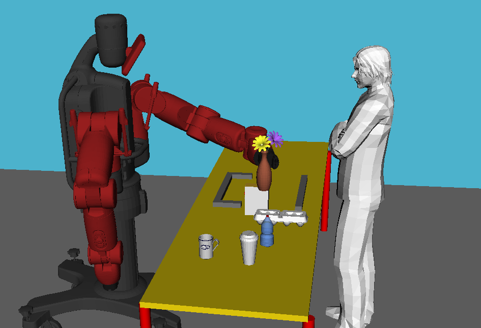
(a) Moving flower vase

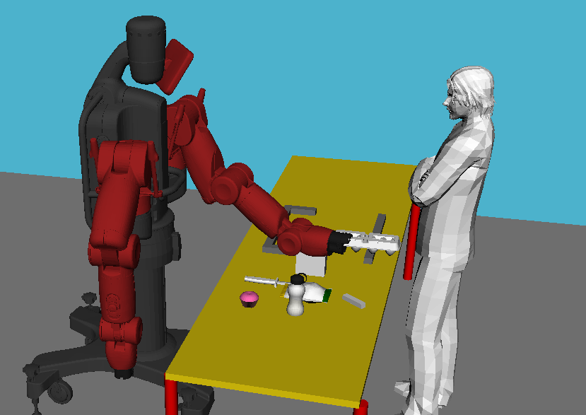
(b) Checking out eggs

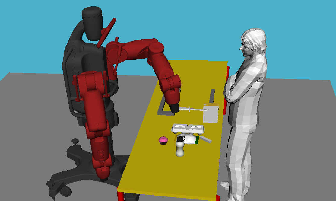
(c) Manipulating knife

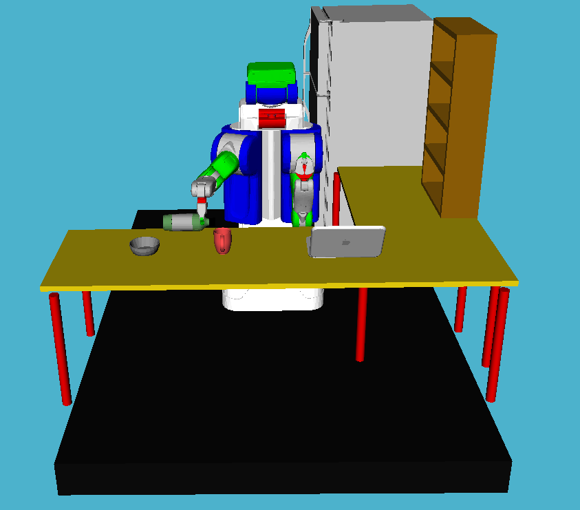
(a) Pouring water

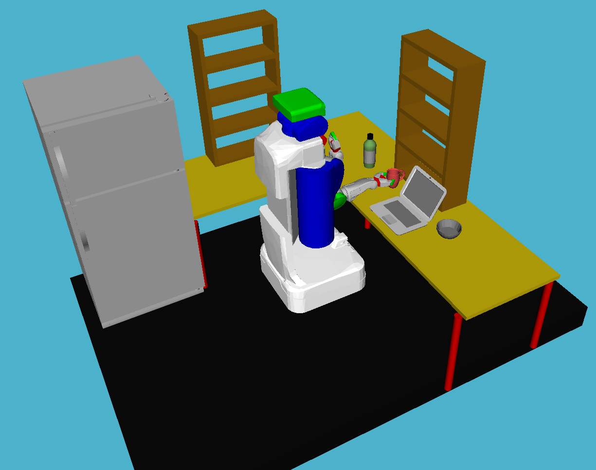
(b) Moving liquid near laptop

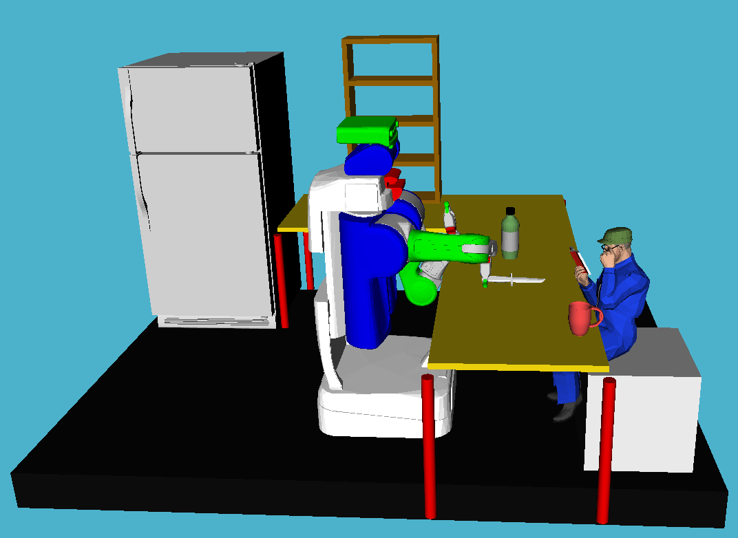
(c) Manipulating sharp object

Figure 8: Robot demonstrating different grocery store and household activities with various objects (Left) Manipulation centric: while pouring water the tilt angle of bottle must change in a particular manner, similarly a flower vase should be kept upright. (Middle) Environment centric: laptop is an electronic device so robot must carefully move water near it, similarly eggs are fragile and should not be lifted too high. (Right) Human centric: knife is sharp and interacts with nearby soft items and humans. It should strictly be kept at a safe distance from humans. (Best viewed in color)

1. Manipulation centric: These activities are primarily concerned with the object being manipulated. Hence the object’s properties and the way the robot moves it in the environment are more relevant. Examples of such household activities are pouring water into a cup or inserting pen into a pen holder, as in Figure 8 (Left). While in a grocery store, such activities could include moving a flower vase or moving fruits and vegetables, which could be damaged when dropped or pushed into other items. We consider pick-and-place, pouring and inserting activities with following objects: cup, bowl, bottle, pen, cereal box, flower vase, and tomato. Further, in every environment we place many objects, along with the object to be manipulated, to restrict simple straight line trajectories.

2. Environment centric: These activities are also concerned with the interactions of the object being manipulated with the surrounding objects. Our object-object interaction features (Section V-A) allow the algorithm to learn preferences on trajectories for moving fragile objects like egg cartons or moving liquid near electronic devices, as in Figure 8 (Middle). We consider moving fragile items like egg carton, heavy metal boxes near a glass table, water near laptop and other electronic devices.

3. Human centric: Sudden movements by the robot put the human in danger of getting hurt. We consider activities where a robot manipulates sharp objects such as knife, as in Figure 8 (Right), moves a hot coffee cup or a bowl of water with a human in vicinity.

Experiment setting. Through experiments we will study:

• Generalization: Performance of robot on tasks that it has not seen before.

• No demonstrations: Comparison of TPP to algorithms that also learn in absence of expert’s demonstrations.

• Feedback: Effectiveness of different kinds of user feedback in absence of expert’s demonstrations.

	Same environment, different object.	New Environment, same object.	New Environment, different object.
nDCG@3

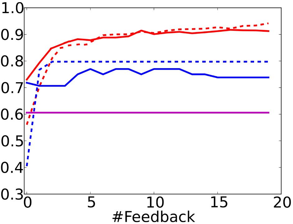
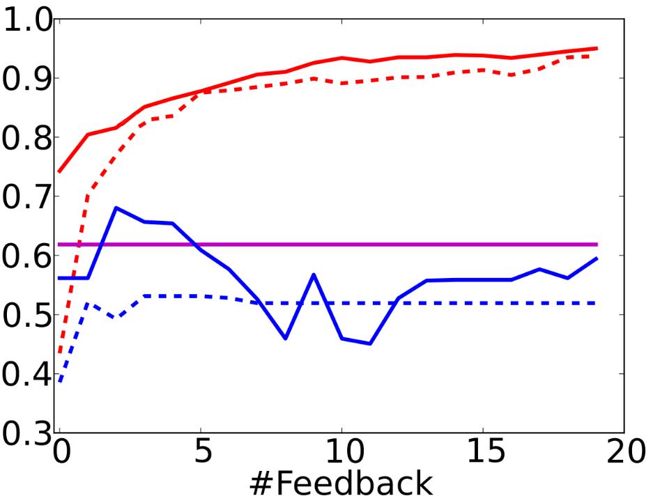
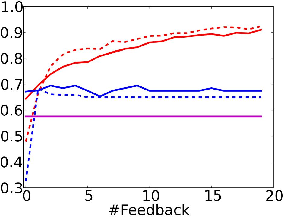
Results on Baxter in grocery store setting.

nDCG@3

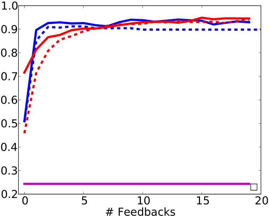
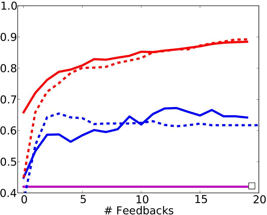
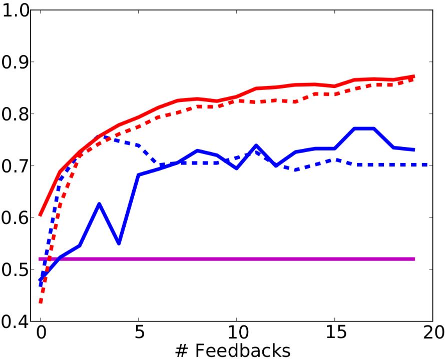
Results on PR2 in household setting.

Figure 9: Study of generalization with change in object, environment and both. Manual, Pre-trained MMP-online (—), Untrained MMP-online (– –), Pre-trained TPP (—), Untrained TPP (– –).

Baseline algorithms. We evaluate algorithms that learn preferences from online feedback under two settings: (a) untrained, where the algorithms learn preferences for a new task from scratch without observing any previous feedback; (b) pre-trained, where the algorithms are pre-trained on other similar tasks, and then adapt to a new task. We compare the following algorithms:

• Geometric: The robot plans a path, independent of the task, using a Bi-directional RRT (BiRRT) [33] planner.

• Manual: The robot plans a path following certain manually coded preferences.

• TPP: Our algorithm, evaluated under both untrained and pre-trained settings.

• MMP-online: This is an online implementation of the Maximum Margin Planning (MMP) [44, 46] algorithm. MMP attempts to make an expert’s trajectory better than any other trajectory by a margin. It can be interpreted as a special case of our algorithm with 1-informative i.e. optimal feedback. However, directly adapting MMP [44] to our experiments poses two challenges: (i) we do not have knowledge of the optimal trajectory; and (ii) the state space of the manipulator we consider is too large, discretizing which makes intractable to train MMP.

  To ensure a fair comparison, we follow the MMP algorithm from [44, 46] and train it under similar settings as TPP. Algorithm 2 shows our implementation of MMP-online. It is very similar to TPP (Algorithm LABEL:alg:coactive) but with a different parameter update step. Since both algorithms only observe user feedback and not demonstrations, MMP-online treats each feedback as a proxy for optimal demonstration. At every iteration MMP-online trains a structural support vector machine (SSVM) [25] using all previous feedback as training examples, and use the learned weights to predict trajectory scores in the next iteration. Since the argmax operation is performed on a set of trajectories it remains tractable. We quantify closeness of trajectories by the $L_{2}-$norm of the difference in their feature representations, and choose the regularization parameter $C$ for training SSVM in hindsight, giving an unfair advantage to MMP-online.

Algorithm 2 MMP-online

  Initialize ${w}_{O}^{(1)}\leftarrow 0$, ${w}_{E}^{(1)}\leftarrow 0,\mathcal{T}=\{\}$

  for $t=1\;\text{to}\;T$ do

     Sample trajectories $\{y^{(1)},...,y^{(n)}\}$

     ${y}_{t}=argmax_{{y}}s(x_{t},{y};w_{O}^{(t)},w_{E}^{(t)})$

     Obtain user feedback $\bar{{y}}_{t}$

     $\mathcal{T}=\mathcal{T}\cup\{(x_{t},\bar{y}_{t})\}$

     $w_{O}^{(t+1)},w_{E}^{(t+1)}=\text{Train-SSVM}(\mathcal{T})$ (Joachims et al. [25])

  end for

Evaluation metrics. In addition to performing a user study (Section VI-D), we also designed two datasets to quantitatively evaluate the performance of our online algorithm. We obtained experts labels on 1300 trajectories in a grocery setting and 2100 trajectories in a household setting. Labels were on the basis of subjective human preferences on a Likert scale of 1-5 (where 5 is the best). Note that these absolute ratings are never provided to our algorithms and are only used for the quantitative evaluation of different algorithms.

We evaluate performance of algorithms by measuring how well they rank trajectories, that is, trajectories with higher Likert score should be ranked higher. To quantify the quality of a ranked list of trajectories we report normalized discounted cumulative gain (nDCG) [38] — criterion popularly used in Information Retrieval for document ranking. In particular we report nDCG at positions 1 and 3, equation (6). While nDCG@1 is a suitable metric for autonomous robots that execute the top ranked trajectory (e.g., grocery checkout), nDCG@3 is suitable for scenarios where the robot is supervised by humans, (e.g., assembly lines). For a given ranked list of items (trajectories here) nDCG at position $k$ is defined as:

$$DCG@k =\sum_{i=1}^{k}\frac{l_{i}}{\log_{2}(i+1)}$$ (5)

$$nDCG@k =\frac{DCG@k}{IDCG@k},$$ (6)

where $l_{i}$ is the Likert score of the item at position $i$ in the ranked list. $IDCG$ is the $DCG$ value of the best possible ranking of items. It is obtained by ranking items in decreasing order of their Likert score.

VI-B Results and Discussion

We now present quantitative results where we compare TPP against the baseline algorithms on our data set of labeled trajectories.
 
  How well does TPP generalize to new tasks? To study generalization of preference feedback we evaluate performance of TPP-pre-trained (i.e., TPP algorithm under pre-trained setting) on a set of tasks the algorithm has not seen before. We study generalization when: (a) only the object being manipulated changes, e.g., a bowl replaced by a cup or an egg carton replaced by tomatoes, (b) only the surrounding environment changes, e.g., rearranging objects in the environment or changing the start location of tasks, and (c) when both change. Figure 9 shows nDCG@3 plots averaged over tasks for all types of activities for both household and grocery store settings. TPP-pre-trained starts-off with higher nDCG@3 values than TPP-untrained in all three cases. However, as more feedback is provided, the performance of both algorithms improves, and they eventually give identical performance. We further observe that generalizing to tasks with both new environment and object is harder than when only one of them changes.
 
  How does TPP compare to MMP-online? MMP-online while training assumes all user feedback is optimal, and hence over time it accumulates many contradictory/sub-optimal training examples. We empirically observe that MMP-online generalizes better in grocery store setting than the household setting (Figure 9), however under both settings its performance remains much lower than TPP. This also highlights the sensitivity of MMP to sub-optimal demonstrations.
 
  How does TPP compare to Manual? For the manual baseline we encode some preferences into the planners, e.g., keep a glass of water upright. However, some preferences are difficult to specify, e.g., not to move heavy objects over fragile items. We empirically found (Figure 9) that the resultant manual algorithm produces poor trajectories in comparison with TPP, with an average nDCG@3 of 0.44 over all types of household activities. Table I reports nDCG values averaged over 20 feedback iterations in untrained setting. For both household and grocery activities, TPP performs better than other baseline algorithms.
 

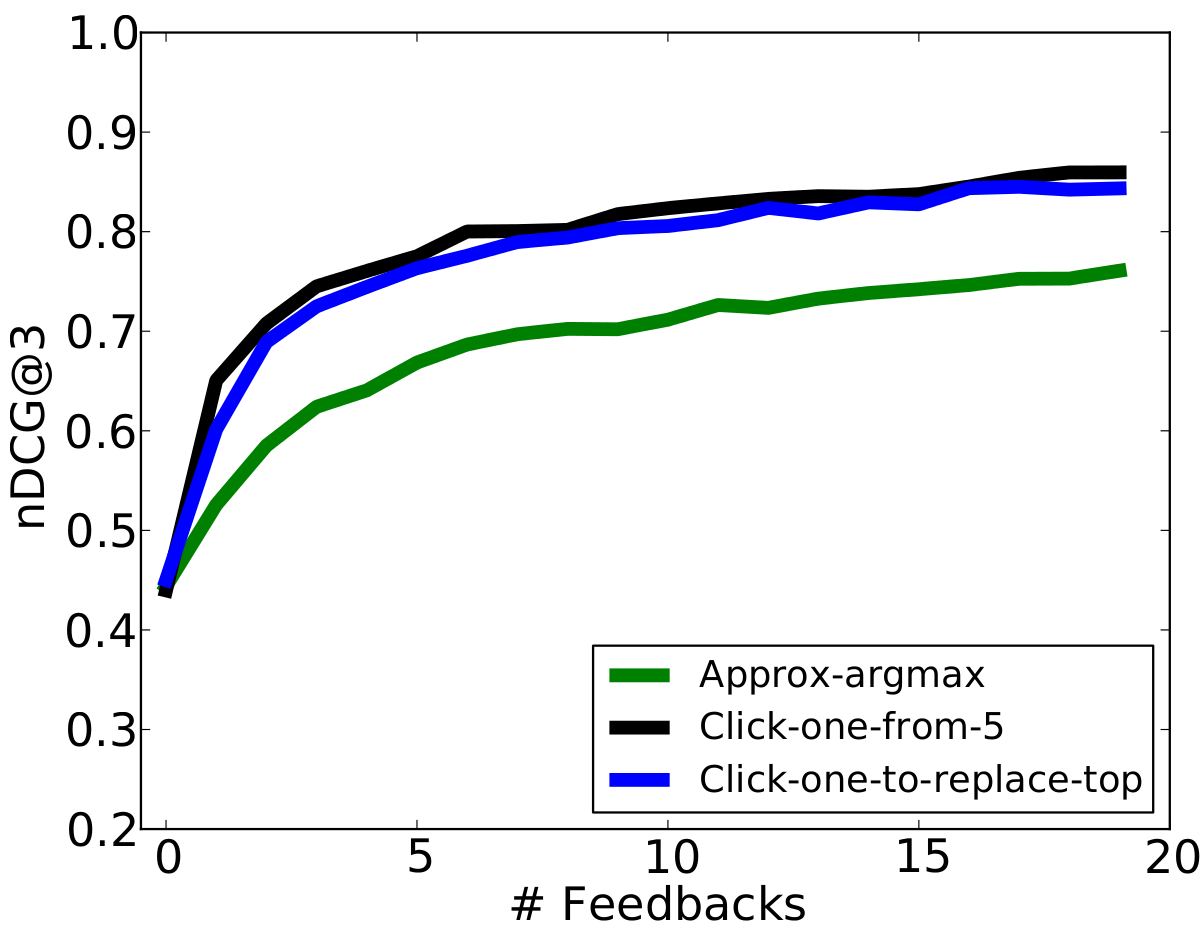
Figure 10: Study of re-rank feedback on Baxter for grocery store setting.

How does TPP perform with weaker feedback? To study the robustness of TPP to less informative feedback we consider the following variants of re-rank feedback:

• Click-one-to-replace-top: User observes the trajectories sequentially in order of their current predicted scores and clicks on the first trajectory which is better than the top ranked trajectory.

• Click-one-from-5: Top $5$ trajectories are shown and user clicks on the one he thinks is the best after watching all $5$ of them.

• Approximate-argmax: This is a weaker feedback, here instead of presenting top ranked trajectories, five random trajectories are selected as candidate. The user selects the best trajectory among these 5 candidates. This simulates a situation when computing an argmax over trajectories is prohibitive and therefore approximated.

		Grocery store setting on Baxter.				Household setting on PR2.
	Algorithms	Manip.	Environ.	Human	Mean	Manip.	Environ.	Human	Mean
		centric	centric	centric		centric	centric	centric
	Geometric	.46 (.48)	.45 (.39)	.31 (.30)	.40 (.39)	.36 (.54)	.43 (.38)	.36 (.27)	.38 (.40)
	Manual	.61 (.62)	.77 (.77)	.33 (.31)	.57 (.57)	.53 (.55)	.39 (.53)	.40 (.37)	.44 (.48)
	MMP-online	.47 (.50)	.54 (.56)	.33 (.30)	.45 (.46)	.83 (.82)	.42 (.51)	.36 (.33)	.54 (.55)
	TPP	.88 (.84)	.90 (.85)	.90 (.80)	.89 (.83)	.93 (.92)	.85 (.75)	.78 (.66)	.85 (.78)

Table I: Comparison of different algorithms in untrained setting. Table contains nDCG@1(nDCG@3) values averaged over 20 feedbacks.

Figure 10 shows the performance of TPP-untrained receiving different kinds of feedback and averaged over three types of activities in grocery store setting. When feedback is more $\alpha$-informative the algorithm requires fewer iterations to learn preferences. In particular, click-one-to-replace-top and click-one-from-5 are more informative than approximate-argmax and therefore require less feedback to reach a given nDCG@1 value. Approximate-argmax improves slowly since it is least informative. In all three cases the feedback is $\alpha$-informative, for some $\alpha>0$, therefore TPP-untrained eventually learns the user’s preferences.

VI-C Comparison with fully-supervised algorithms

The algorithms discussed so far only observes ordinal feedback where the users iteratively improves upon the proposed trajectory. In this section we compare TPP to a fully-supervised algorithm that observes expert’s labels while training. Eliciting such expert labels on the large space of trajectories is not realizable in practice. However, empirically it nonetheless provides an upper-bound on the generalization to new tasks. We refer to this algorithm as Oracle-svm and it learns to rank trajectories using SVM-rank [24]. Since expert labels are not available while prediction, on test set Oracle-svm predicts once and does not learn from user feedback.

Figure 11 compares TPP and Oracle-svm on new tasks. Without observing any feedback on new tasks Oracle-svm performs better than TPP. However, after few feedback iterations TPP improves over Oracle-svm, which is not updated since it requires expert’s labels on test set. On average, we observe, it takes 5 feedback iterations for TPP to improve over Oracle-svm. Furthermore, learning from demonstration (LfD) can be seen as a special case of Oracle-svm where, instead of providing an expert label for every sampled trajectory, the expert directly demonstrates the optimal trajectory.

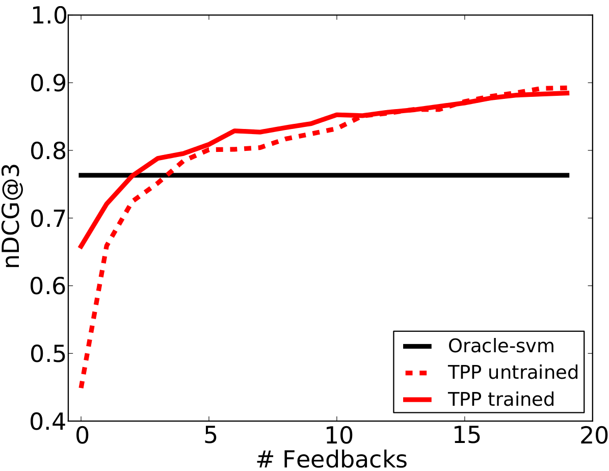
Figure 11: Comparision with fully-supervised Oracle-svm on Baxter for grocery store setting.

VI-D Robotic Experiment: User Study in learning trajectories

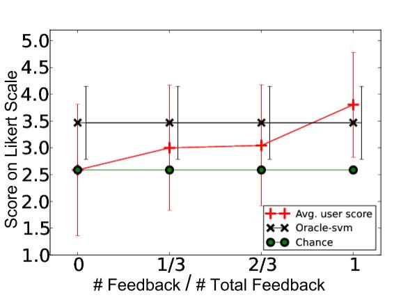
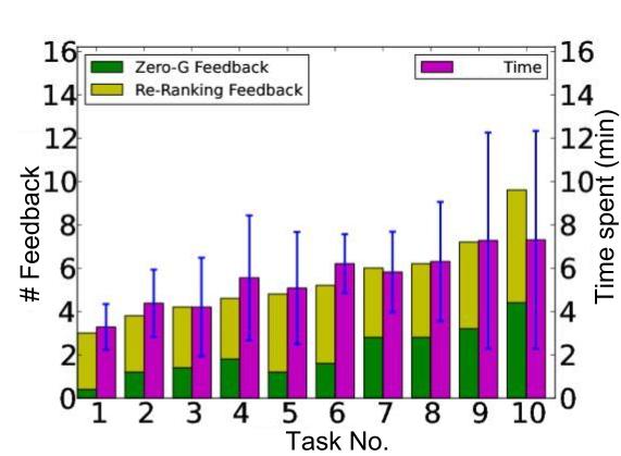
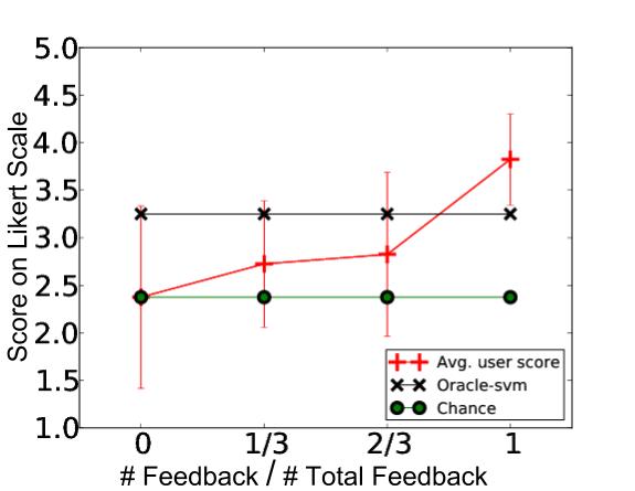
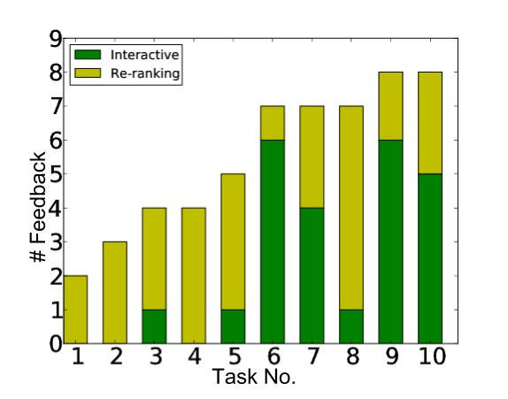
Grocery store setting on Baxter.

Household setting on PR2.

Figure 12: (Left) Average quality of the learned trajectory after every one-third of total feedback. (Right) Bar chart showing the average number of feedback (re-ranking and zero-G) and time required (only for grocery store setting) for each task. Task difficulty increases from 1 to 10.

We perform a user study of our system on Baxter and PR2 on a variety of tasks of varying difficulties in grocery store and household settings, respectively. Thereby we show a proof-of-concept of our approach in real world robotic scenarios, and that the combination of re-ranking and zero-G/interactive feedback allows users to train the robot in few feedback iterations.
 
  Experiment setup: In this study, users not associated with this work, used our system to train PR2 and Baxter on household and grocery checkout tasks, respectively. Five users independently trained Baxter, by providing zero-G feedback kinesthetically on the robot, and re-rank feedback in a simulator. Two users participated in the study on PR2. On PR2, in place of zero-G, users provided interactive waypoint correction feedback in the Rviz simulator. The users were undergraduate students. Further, both users training PR2 on household tasks were familiar with Rviz-ROS. A set of 10 tasks of varying difficulty level was presented to users one at a time, and they were instructed to provide feedback until they were satisfied with the top ranked trajectory. To quantify the quality of learning each user evaluated their own trajectories (self score), the trajectories learned by the other users (cross score), and those predicted by Oracle-svm, on a Likert scale of 1-5. We also recorded the total time a user spent on each task – from start of training till the user was satisfied with the top ranked trajectory. This includes time taken for both re-rank and zero-G feedback.
 

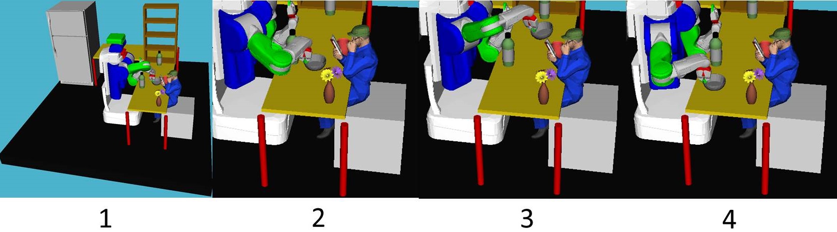
Figure 13: Shows trajectories for moving a bowl of water in presence of human. Without learning robot plans an undesirable trajectory and moves bowl over the human (waypoints 1-3-4). After six user feedback robot learns the desirable trajectory (waypoints 1-2-4).

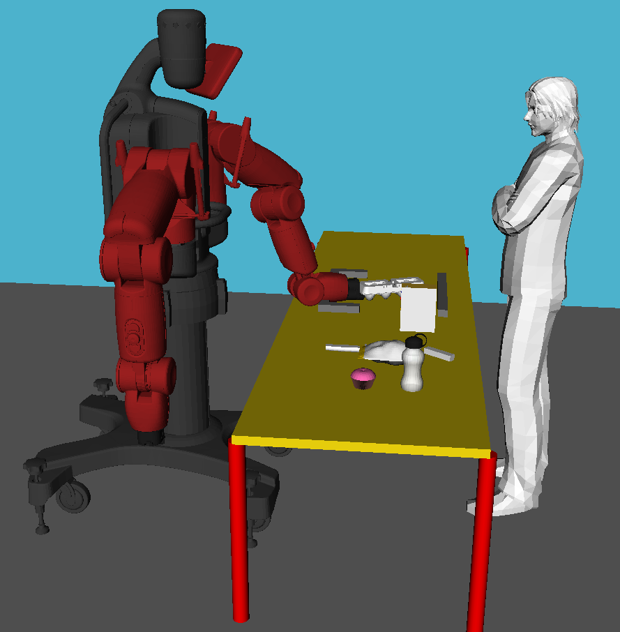
Figure 14: Shows the learned trajectory for moving an egg carton. Since eggs are fragile robot moves the carton near the table surface. (Left) Start of trajectory. (Middle) Intermediate waypoint with egg close to the table surface. (Right) End of trajectory.

Is re-rank feedback easier to elicit from users than zero-G or interactive? In our user study, on average a user took 3 re-rank and 2 zero-G feedback per task to train a robot (Table II). From this we conjecture, that for high DoF manipulators re-rank feedback is easier to provide than zero-G – which requires modifying the manipulator joint angles. However, an increase in the count of zero-G (interactive) feedback with task difficulty suggests (Figure 12 (Right)), users rely more on zero-G feedback for difficult tasks since it allows precisely rectifying erroneous waypoints. Figure 13 and Figure 14 show two example trajectories learned by a user.
 
  How many feedback iterations a user takes to improve over Oracle-svm? Figure 12 (Left) shows that the quality of trajectory improves with feedback. On average, a user took 5 feedback to improve over Oracle-svm, which is also consistent with our quantitative analysis (Section VI-C). In grocery setting, users 4 and 5 were critical towards trajectories learned by Oracle-svm and gave them low scores. This indicates a possible mismatch in preferences between our expert (on whose labels Oracle-svm was trained) and users 4 and 5.

User	# Re-ranking	# Zero-G	Average	Trajectory-Quality
	feedback	feedback	time (min.)	self	cross
1	5.4 (4.1)	3.3 (3.4)	7.8 (4.9)	3.8 (0.6)	4.0 (1.4)
2	1.8 (1.0)	1.7 (1.3)	4.6 (1.7)	4.3 (1.2)	3.6 (1.2)
3	2.9 (0.8)	2.0 (2.0)	5.0 (2.9)	4.4 (0.7)	3.2 (1.2)
4	3.2 (2.0)	1.5 (0.9)	5.3 (1.9)	3.0 (1.2)	3.7 (1.0)
5	3.6 (1.0)	1.9 (2.1)	5.0 (2.3)	3.5 (1.3)	3.3 (0.6)

User	# Re-ranking	# Interactive	Trajectory-Quality
	feedbacks	feedbacks	self	cross
1	3.1 (1.3)	2.4 (2.4)	3.5 (1.1)	3.6 (0.8)
2	2.3 (1.1)	1.8 (2.7)	4.1 (0.7)	4.1 (0.5)

Table II: Shows learning statistics for each user. Self and cross scores of the final learned trajectories. The number inside bracket is standard deviation. (Top) Results for grocery store on Baxter. (Bottom) Household setting on PR2.

How do users’ unobserved score functions vary? An average difference of 0.6 between users’ self and cross score (Table II) in the grocery checkout setting suggests preferences varied across users, but only marginally. In situations where this difference is significant and a system is desired for a user population, a future work might explore coactive learning for satisfying user population, similar to Raman and Joachims [42]. For household setting, the sample size is small to draw a similar conclusion.
 
  How long does it take for users to train a robot? We report training time for only the grocery store setting, because the interactive feedback in the household setting requires users with experience in Rviz-ROS. Further, we observed that users found it difficult to modify the robot’s joint angles in a simulator to their desired configuration. In the grocery checkout setting, among all the users, user 1 had the strictest preferences and also experienced some early difficulties in using the system and therefore took longer than others. On an average, a user took 5.5 minutes per task, which we believe is acceptable for most applications. Future research in human-computer interaction, visualization and better user interfaces [52] could further reduce this time. For example, simultaneous visualization of top ranked trajectories instead of sequentially showing them to users (the scheme we currently adopt) could bring down the time for re-rank feedback. Despite its limited size, through our user study we show that our algorithm is realizable in practice on high DoF manipulators. We hope this motivates researchers to build robotic systems capable of learning from non-expert users. For more details, videos and code, visit:

http://pr.cs.cornell.edu/coactive/

VII Conclusion and Future work

When manipulating objects in human environments, it is important for robots to plan motions that follow users’ preferences. In this work, we considered preferences that go beyond simple geometric constraints and that considered surrounding context of various objects and humans in the environment. We presented a coactive learning approach for teaching robots these preferences through iterative improvements from non-expert users. Unlike in standard learning from demonstration approaches, our approach does not require the user to provide optimal trajectories as training data. We evaluated our approach on various household (with PR2) and grocery store checkout (with Baxter) settings. Our experiments suggest that it is indeed possible to train robots within a few minutes with just a few incremental feedbacks from non-expert users.

Future research could extend coactive learning to situations with uncertainty in object pose and attributes. Under uncertainty the trajectory preference perceptron will admit a belief space update form, and theoretical guarantees will also be different. Coactive feedback might also find use in other interesting robotic applications such as assistive cars, where a car learns from humans steering actions. Scaling up coactive feedback by crowd-sourcing and exploring other forms of easy-to-elicit learning signals are also potential future directions.

Appendix A Proof for Average Regret

This proof builds upon Shivaswamy & Joachims [51].

We assume the user hidden score function $s^{*}(x,{y})$ is contained in the family of scoring functions $s(x,{y};w_{O}^{*},w_{E}^{*})$ for some unknown $w_{O}^{*}$ and $w_{E}^{*}$. Average regret for TPP over $T$ rounds of interactions can be written as:

$$REG_{T} =\frac{1}{T}\sum_{t=1}^{T}({s}^{*}(x_{t},{{y}}_{t}^{*})-{s}^{*}(x_{t},{{y}}_{t}))$$

$$=\frac{1}{T}\sum_{t=1}^{T}({s}(x_{t},{{y}}_{t}^{*};w_{O}^{*},w_{E}^{*})-{s}(x_{t},{{y}}_{t};w_{O}^{*},w_{E}^{*}))$$

We further assume the feedback provided by the user is strictly $\alpha$-informative and satisfy following inequality:

$$s(x_{t},\bar{y}_{t};w_{O}^{*},w_{E}^{*})\geq s(x_{t},y_{t};w_{O}^{*},w_{E}^{*})+\alpha[{s}(x_{t},{{y}}_{t}^{*};w_{O}^{*},w_{E}^{*})$$

$$-{s}(x_{t},{{y}}_{t};w_{O}^{*},w_{E}^{*})]-\xi_{t}$$ (7)

Later we relax this constraint and requires it to hold only in expectation.

This definition states that the user feedback should have a score of $\bar{y}_{t}$ that is higher than that of $y_{t}$ by a fraction $\alpha\in(0,1]$ of the maximum possible range $s(x_{t},y_{t}^{*};w_{O}^{*},w_{E}^{*})-s(x_{t},y_{t};w_{O}^{*},w_{E}^{*})$.
 

Theorem 1

The average regret of trajectory preference perceptron receiving strictly $\alpha$-informative feedback can be upper bounded for any $[{w}_{O}^{*};{w}_{E}^{*}]$ as follows:

$$REG_{T}\leq\frac{2C\left\|[{w}_{O}^{*};{w}_{E}^{*}]\right\|}{\alpha\sqrt{T}}+\frac{1}{\alpha T}\sum_{t=1}^{T}\xi_{t}$$ (8)

where C is constant such that $\left\|\left[\phi_{O}(x,{y});\phi_{E}(x,{y})\right]\right\|_{2}\leq C$.

Proof: After $T$ rounds of feedback, using weight update equations of $w_{E}$ and $w_{O}$ we can write:

$${w}_{O}^{*}\cdot{w}_{O}^{(T+1)} ={w}_{O}^{*}\cdot{w}_{O}^{(T)}+{w}_{O}^{*}\cdot({\phi_{O}}(x_{T},{\bar{{y}}_{T}})-{\phi_{O}}(x_{T},{{y}_{T}}))$$

$${w}_{E}^{*}\cdot{w}_{E}^{(T+1)} ={w}_{E}^{*}\cdot{w}_{E}^{(T)}+{w}_{E}^{*}\cdot({\phi_{E}}(x_{T},{\bar{{y}}_{T}})-{\phi_{E}}(x_{T},{{y}_{T}}))$$

Adding the two equations and recursively reducing the right gives:

$${w}_{O}^{*}\cdot{w}_{O}^{(T+1)}+{w}_{E}^{*}\cdot{w}_{E}^{(T+1)}= \sum_{t=1}^{T}({s}(x_{t},{\bar{y}}_{t};w_{O}^{*},w_{E}^{*})$$

$$-{s}(x_{t},{{y}}_{t};w_{O}^{*},w_{E}^{*}))$$ (9)

Using Cauchy-Schwarz inequality the left hand side of equation (A) can be bounded as:

$${w}_{O}^{*}\cdot{w}_{O}^{(T+1)}+{w}_{E}^{*}\cdot{w}_{E}^{(T+1)}\leq\left\|[{w}_{O}^{*};{w}_{E}^{*}]\right\|\left\|[{w}_{O}^{(T+1)};{w}_{E}^{(T+1)}]\right\|\\$$ (10)

$\left\|[{w}_{O}^{(T+1)};{w}_{E}^{(T+1)}]\right\|$ can be bounded by using weight update equations:

$${w}_{O}^{(T+1)}\cdot{w}_{O}^{(T+1)}+{w}_{E}^{(T+1)}\cdot{w}_{E}^{(T+1)}={w}_{O}^{(T)}\cdot{w}_{O}^{(T)}+{w}_{E}^{(T)}\cdot{w}_{E}^{(T)}$$

$$+2{w}_{O}^{(T)}\cdot({\phi_{O}}(x_{T},{\bar{{y}}_{T}})-{\phi_{O}}(x_{T},{{y}_{T}}))$$

$$+2{w}_{E}^{(T)}\cdot({\phi_{E}}(x_{T},{\bar{{y}}_{T}})-{\phi_{E}}(x_{T},{{y}_{T}}))$$

$$+({\phi_{O}}(x_{T},{\bar{{y}}_{T}})-{\phi_{O}}(x_{T},{{y}_{T}}))\cdot({\phi_{O}}(x_{T},{\bar{{y}}_{T}})-{\phi_{O}}(x_{T},{{y}_{T}}))$$

$$+({\phi_{E}}(x_{T},{\bar{{y}}_{T}})-{\phi_{E}}(x_{T},{{y}_{T}}))\cdot({\phi_{E}}(x_{T},{\bar{{y}}_{T}})-{\phi_{E}}(x_{T},{{y}_{T}}))$$

$$\leq{w}_{O}^{(T)}\cdot{w}_{O}^{(T)}+{w}_{E}^{(T)}\cdot{w}_{E}^{(T)}+4C^{2}\leq 4C^{2}T$$ (11)

$$\therefore\left\|[{w}_{O}^{(T+1)};{w}_{E}^{(T+1)}]\right\|\leq 2C\sqrt{T}$$ (12)

Eq. (11) follows from the fact that $s(x_{T},{{y}}_{T};w_{O}^{(T)},w_{E}^{(T)})>s(x_{T},\bar{{y}}_{T};w_{O}^{(T)},w_{E}^{(T)})$ and $\left\|\left[\phi_{O}(x,{y});\phi_{E}(x,{y})\right]\right\|_{2}\leq C$. Using equations (10) and (12) gives following bound on (A):

$$\sum_{t=1}^{T}({s}(x_{t},{\bar{y}}_{t};w_{O}^{*},w_{E}^{*})-{s}( x_{t},{{y}}_{t};w_{O}^{*},w_{E}^{*}))$$

$$\leq 2C\sqrt{T}\left\|[{w}_{O}^{*};{w}_{E}^{*}]\right\|$$ (13)

Assuming strictly $\alpha$-informative feedback and re-writing equation (A) as:

$$s(x_{t},{y}_{t}^{*};w_{O}^{*},w_{E}^{*})-s(x_{t},y_{t};w_{O}^{*},w_{E}^{*})$$

$$\leq\frac{1}{\alpha}(({s}(x_{t},{\bar{y}}_{t};w_{O}^{*},w_{E}^{*})-{s}(x_{t},{{y}}_{t};w_{O}^{*},w_{E}^{*}))-\xi_{t})$$ (14)

Combining equations (A) and (A) gives the bound on average regret (8).

Appendix B Proof for Expected Regret

We now show the regret bounds for TPP under a weaker feedback assumption – expected $\alpha$-informative feedback:

$$E_{t}[s(x_{t},\bar{y}_{t}; w_{O}^{*},w_{E}^{*})]\geq s(x_{t},y_{t};w_{O}^{*},w_{E}^{*})$$

$$+\alpha[{s}(x_{t},{{y}}_{t}^{*};w_{O}^{*},w_{E}^{*})-{s}(x_{t},{{y}}_{t};w_{O}^{*},w_{E}^{*})]-\xi_{t}$$

where the expectation is under choices $\bar{y}_{t}$ when $y_{t}$ and $x_{t}$ are known.

Corollary 2

The expected regret of trajectory preference perceptron receiving expected $\alpha$-informative feedback can be upper bounded for any $[{w}_{O}^{*};{w}_{E}^{*}]$ as follows:

$$E[REG_{T}]\leq\frac{2C\left\|[{w}_{G}^{*};{w}_{O}^{*}]\right\|}{\alpha\sqrt{T}}+\frac{1}{\alpha T}\sum_{t=1}^{T}\bar{\xi}_{t}$$ (15)

Proof: Taking expectation on both sides of equation (A), (10) and (11) yields following equations respectively:

$$E[{w}_{O}^{*}\cdot{w}_{O}^{(T+1)}+{w}_{E}^{*}\cdot{w}_{E}^{(T+1)}] =\sum_{t=1}^{T}E[({s}(x_{t},{\bar{y}}_{t};w_{O}^{*},w_{E}^{*})$$

$$-{s}(x_{t},{{y}}_{t};w_{O}^{*},w_{E}^{*}))]$$ (16)

$$E[{w}_{O}^{*}\cdot{w}_{O}^{(T+1)}+ {w}_{E}^{*}\cdot{w}_{E}^{(T+1)}]$$

$$\leq\left\|[{w}_{O}^{*};{w}_{E}^{*}]\right\|E\left[\left\|[{w}_{O}^{(T+1)};{w}_{E}^{(T+1)}]\right\|\right]$$

$$E[{w}_{O}^{(T+1)}\cdot{w}_{O}^{(T+1)}+{w}_{E}^{(T+1)}\cdot{w}_{E}^{(T+1)}]\leq 4C^{2}T$$

Applying Jensen’s inequality on the concave function $\sqrt{\cdot}$ we get:

$$E[{w}_{O}^{*}\cdot{w}_{O}^{(T+1)}+{w}_{E}^{*}\cdot{w}_{E}^{(T+1)}]$$

$$\leq\left\|[{w}_{O}^{*};{w}_{E}^{*}]\right\|E\left[\left\|[{w}_{O}^{(T+1)};{w}_{E}^{(T+1)}]\right\|\right]$$

$$\leq\left\|[{w}_{O}^{*};{w}_{E}^{*}]\right\|\sqrt{E[{w}_{O}^{(T+1)}\cdot{w}_{O}^{(T+1)}+{w}_{E}^{(T+1)}\cdot{w}_{E}^{(T+1)}]}$$

Using (B) gives the following bound:

$$\sum_{t=1}^{T}E[{s}(x_{t},{\bar{y}}_{t};w_{O}^{*},w_{E}^{*}) -{s}(x_{t},{{y}}_{t};w_{O}^{*},w_{E}^{*})]$$

$$\leq 2C\sqrt{T}\left\|[{w}_{O}^{*};{w}_{E}^{*}]\right\|$$

Now using the fact that the user feedback is expected $\alpha$-informative gives the regret bound (15).

References

- Abbeel et al. [2010] P. Abbeel, A. Coates, and A. Y. Ng. Autonomous helicopter aerobatics through apprenticeship learning. International Journal of Robotics Research, 29(13), 2010.
- Akgun et al. [2012] B. Akgun, M. Cakmak, K. Jiang, and A. L. Thomaz. Keyframe-based learning from demonstration. International Journal of Social Robotics, 4(4):343–355, 2012.
- Alterovitz et al. [2007] R. Alterovitz, T. Siméon, and K. Goldberg. The stochastic motion roadmap: A sampling framework for planning with markov motion uncertainty. In Proceedings of Robotics: Science and Systems, 2007.
- Argall et al. [2009] B. D. Argall, S. Chernova, M. Veloso, and B. Browning. A survey of robot learning from demonstration. Robotics and Autonomous Systems, 57(5):469–483, 2009.
- Berenson et al. [2012] D. Berenson, P. Abbeel, and K. Goldberg. A robot path planning framework that learns from experience. In Proceedings of the International Conference on Robotics and Automation, 2012.
- Berg et al. [2010] J. V. D. Berg, P. Abbeel, and K. Goldberg. Lqg-mp: Optimized path planning for robots with motion uncertainty and imperfect state information. In Proceedings of Robotics: Science and Systems, June 2010.
- Bhattacharya et al. [2011] S. Bhattacharya, M. Likhachev, and V. Kumar. Identification and representation of homotopy classes of trajectories for search-based path planning in 3d. In Proceedings of Robotics: Science and Systems, 2011.
- Bischoff et al. [2002] R. Bischoff, A. Kazi, and M. Seyfarth. The morpha style guide for icon-based programming. In Proceedings. 11th IEEE International Workshop on RHIC., 2002.
- Calinon et al. [2007] S. Calinon, F. Guenter, and A. Billard. On learning, representing, and generalizing a task in a humanoid robot. Sys., Man, and Cybernetics, Part B: Cybernetics, IEEE Trans. on, 2007.
- Cohen et al. [2010] B. J. Cohen, S. Chitta, and M. Likhachev. Search-based planning for manipulation with motion primitives. In Proceedings of the International Conference on Robotics and Automation, pages 2902–2908, 2010.
- D. Ferguson and Stentz [2006] Dave D. Ferguson and A. Stentz. Anytime rrts. In Proceedings of the IEEE/RSJ Conference on Intelligent Robots and Systems, 2006.
- Dey et al. [2012] D. Dey, T. Y. Liu, M. Hebert, and J. A. Bagnell. Contextual sequence prediction with application to control library optimization. In Proceedings of Robotics: Science and Systems, 2012.
- Diankov [2010] R. Diankov. Automated Construction of Robotic Manipulation Programs. PhD thesis, CMU, RI, August 2010.
- Dragan and Srinivasa [2013] A. Dragan and S. Srinivasa. Generating legible motion. In Proceedings of Robotics: Science and Systems, 2013.
- Dragan et al. [2013] A. Dragan, K. Lee, and S. Srinivasa. Legibility and predictability of robot motion. In Human Robot Interaction, 2013.
- Erickson and LaValle [2009] L. H. Erickson and S. M. LaValle. Survivability: Measuring and ensuring path diversity. In Proceedings of the International Conference on Robotics and Automation, 2009.
- Ettlin and Bleuler [2006] A. Ettlin and H. Bleuler. Randomised rough-terrain robot motion planning. In Proceedings of the IEEE/RSJ Conference on Intelligent Robots and Systems, 2006.
- Gossow et al. [2011] D. Gossow, A. Leeperand D. Hershberger, and M. Ciocarlie. Interactive markers: 3-d user interfaces for ros applications [ros topics]. Robotics & Automation Magazine, IEEE, 18(4):14–15, 2011.
- Green and Kelly [2011] C. J. Green and A. Kelly. Toward optimal sampling in the space of paths. In Robotics Research. 2011.
- Jaillet et al. [2010] L. Jaillet, J. Cortés, and T. Siméon. Sampling-based path planning on configuration-space costmaps. 26(4), 2010.
- Jain et al. [2013a] A. Jain, S. Sharma, and A. Saxena. Beyond geometric path planning: Learning context-driven user preferences via sub-optimal feedback. In Proceedings of the International Symposium on Robotics Research, 2013a.
- Jain et al. [2013b] A. Jain, B. Wojcik, T. Joachims, and A. Saxena. Learning trajectory preferences for manipulators via iterative improvement. In Advances in Neural Information Processing Systems, 2013b.
- Jiang et al. [2012] Y. Jiang, M. Lim, C. Zheng, and A. Saxena. Learning to place new objects in a scene. International Journal of Robotics Research, 31(9):1021–1043, 2012.
- Joachims [2006] T. Joachims. Training linear svms in linear time. In Proceedings of the ACM Special Interest Group on Knowledge Discovery and Data Mining, 2006.
- Joachims et al. [2009] T. Joachims, T. Finley, and C.-N. J. Yu. Cutting-plane training of structural svms. Machine Learning, 77(1):27–59, 2009.
- Karaman and Frazzoli [2010] S. Karaman and E. Frazzoli. Incremental sampling-based algorithms for optimal motion planning. In Proceedings of Robotics: Science and Systems, 2010.
- Karaman and Frazzoli [2011] S. Karaman and E. Frazzoli. Sampling-based algorithms for optimal motion planning. International Journal of Robotics Research, 30(7):846–894, 2011.
- Kitani et al. [2012] K. M. Kitani, B. D. Ziebart, J. A. Bagnell, and M. Hebert. Activity forecasting. In Proceedings of the European Conference on Computer Vision. 2012.
- Klingbeil et al. [2011] E. Klingbeil, D. Rao, B. Carpenter, V. Ganapathi, A. Y. Ng, and O. Khatib. Grasping with application to an autonomous checkout robot. In Proceedings of the International Conference on Robotics and Automation, 2011.
- Kober and Peters [2011] J. Kober and J. Peters. Policy search for motor primitives in robotics. ML, 84(1), 2011.
- Koppula et al. [2011] H.S. Koppula, A. Anand, T. Joachims, and A. Saxena. Semantic labeling of 3d point clouds for indoor scenes. In Advances in Neural Information Processing Systems, 2011.
- Kretzschmar et al. [2014] H. Kretzschmar, M. Kuderer, and W. Burgard. Learning to predict trajectories of cooperatively navigating agents. In Proceedings of the International Conference on Robotics and Automation, 2014.
- LaValle and Kuffner [2001] S. M. LaValle and J. J. Kuffner. Randomized kinodynamic planning. International Journal of Robotics Research, 20(5), May 2001.
- Lenz et al. [2013] I. Lenz, H. Lee, and A. Saxena. Deep learning for detecting robotic grasps. In Proceedings of Robotics: Science and Systems, 2013.
- Leven and Hutchinson [2003] P. Leven and S. Hutchinson. Using manipulability to bias sampling during the construction of probabilistic roadmaps. IEEE Trans. on Robotics and Automation, 19(6), 2003.
- Levine and Koltun [2012] S. Levine and V. Koltun. Continuous inverse optimal control with locally optimal examples. In Proceedings of the International Conference on Machine Learning, 2012.
- Mainprice et al. [2011] J. Mainprice, E. A. Sisbot, L. Jaillet, J. Cortés, R. Alami, and T. Siméon. Planning human-aware motions using a sampling-based costmap planner. In Proceedings of the International Conference on Robotics and Automation, 2011.
- Manning et al. [2008] C. D. Manning, P. Raghavan, and H. Schütze. Introduction to information retrieval, volume 1. Cambridge University Press Cambridge, 2008.
- Nikolaidis and Shah [2012] S. Nikolaidis and J. Shah. Human-robot teaming using shared mental models. In HRI, Workshop on Human-Agent-Robot Teamwork, 2012.
- Nikolaidis and Shah [2013] S. Nikolaidis and J. Shah. Human-robot cross-training: Computational formulation, modeling and evaluation of a human team training strategy. In IEEE/ACM ICHRI, 2013.
- Phillips et al. [2012] M. Phillips, B. Cohen, S. Chitta, and M. Likhachev. E-graphs: Bootstrapping planning with experience graphs. In Proceedings of Robotics: Science and Systems, 2012.
- Raman and Joachims [2013] K. Raman and T. Joachims. Learning socially optimal information systems from egoistic users. In Proceedings of the European Conference on Machine Learning, 2013.
- Ratliff [2009] N. Ratliff. Learning to Search: Structured Prediction Techniques for Imitation Learning. PhD thesis, CMU, RI, 2009.
- Ratliff et al. [2006] N. Ratliff, J. A. Bagnell, and M. Zinkevich. Maximum margin planning. In Proceedings of the International Conference on Machine Learning, 2006.
- Ratliff et al. [2007] N. Ratliff, J. A. Bagnell, and M. Zinkevich. (online) subgradient methods for structured prediction. In Proceedings of the International Conference on Artificial Intelligence and Statistics, 2007.
- Ratliff et al. [2009a] N. Ratliff, D. Silver, and J. A. Bagnell. Learning to search: Functional gradient techniques for imitation learning. Autonomous Robots, 27(1):25–53, 2009a.
- Ratliff et al. [2009b] N. Ratliff, M. Zucker, J. A. Bagnell, and S. Srinivasa. Chomp: Gradient optimization techniques for efficient motion planning. In Proceedings of the International Conference on Robotics and Automation, 2009b.
- Ross et al. [2013] S. Ross, J. Zhou, Y. Yue, D. Dey, and J. A. Bagnell. Learning policies for contextual submodular prediction. Proceedings of the International Conference on Machine Learning, 2013.
- Saxena et al. [2008] A. Saxena, J. Driemeyer, and A. Y. Ng. Robotic grasping of novel objects using vision. International Journal of Robotics Research, 27(2):157–173, 2008.
- Schulman et al. [2013] J. Schulman, J. Ho, A. Lee, I. Awwal, H. Bradlow, and P. Abbeel. Finding locally optimal, collision-free trajectories with sequential convex optimization. In Proceedings of Robotics: Science and Systems, 2013.
- Shivaswamy and Joachims [2012] P. Shivaswamy and T. Joachims. Online structured prediction via coactive learning. In Proceedings of the International Conference on Machine Learning, 2012.
- Shneiderman and Plaisant [2010] B. Shneiderman and C. Plaisant. Designing The User Interface: Strategies for Effective Human-Computer Interaction. Addison-Wesley Publication, 2010.
- Silver et al. [2010] D. Silver, J. A. Bagnell, and A. Stentz. Learning from demonstration for autonomous navigation in complex unstructured terrain. International Journal of Robotics Research, 2010.
- Sisbot et al. [2007a] E. A. Sisbot, L. F. Marin, and R. Alami. Spatial reasoning for human robot interaction. In Proceedings of the IEEE/RSJ Conference on Intelligent Robots and Systems, 2007a.
- Sisbot et al. [2007b] E. A. Sisbot, L. F. Marin-Urias, R. Alami, and T. Simeon. A human aware mobile robot motion planner. IEEE Transactions on Robotics, 2007b.
- Stopp et al. [2001] A. Stopp, S. Horstmann, S. Kristensen, and F. Lohnert. Towards interactive learning for manufacturing assistants. In Proceedings. 10th IEEE International Workshop on RHIC., 2001.
- Sucan et al. [2012] I. A. Sucan, M. Moll, and L. E. Kavraki. The Open Motion Planning Library. IEEE Robotics & Automation Magazine, 19(4):72–82, 2012. http://ompl.kavrakilab.org.
- Tamane et al. [2013] K. Tamane, M. Revfi, and T. Asfour. Synthesizing object receiving motions of humanoid robots with human motion database. In Proceedings of the International Conference on Robotics and Automation, 2013.
- Vernaza and Bagnell [2012] P. Vernaza and J. A. Bagnell. Efficient high dimensional maximum entropy modeling via symmetric partition functions. In Advances in Neural Information Processing Systems, 2012.
- Wilson et al. [2012] A. Wilson, A. Fern, and P. Tadepalli. A bayesian approach for policy learning from trajectory preference queries. In Advances in Neural Information Processing Systems, 2012.
- Zacharias et al. [2011] F. Zacharias, C. Schlette, F. Schmidt, C. Borst, J. Rossmann, and G. Hirzinger. Making planned paths look more human-like in humanoid robot manipulation planning. In Proceedings of the International Conference on Robotics and Automation, 2011.
- Ziebart et al. [2008] B. D. Ziebart, A. Maas, J. A. Bagnell, and A. K. Dey. Maximum entropy inverse reinforcement learning. In AAAI, 2008.
- Zucker et al. [2013] M. Zucker, N. Ratliff, A. D. Dragan, M. Pivtoraiko, M. Klingensmith, C. M. Dellin, J. A. Bagnell, and S. .S. Srinivasa. Chomp: Covariant hamiltonian optimization for motion planning. International Journal of Robotics Research, 32, 2013.