Polynomial convergence to equilibrium for a system of interacting particles

Abstract.

We consider a stochastic particle system in which a finite number of particles interact with one another via a common energy tank. Interaction rate for each particle is proportional to the square root of its kinetic energy, as is consistent with analogous mechanical models. Our main result is that the rate of convergence to equilibrium for such a system is $\sim t^{-2}$, more precisely it is faster than a constant times $t^{-2+\varepsilon}$ for any $\varepsilon>0$. A discussion of exponential vs polynomial convergence for similar particle systems is included.

This paper is about dynamical models of (large numbers of) interacting particles, a topic of fundamental importance in both dynamical systems and statistical mechanics. Our focus is on the speed of convergence to equilibrium, equivalently the rate of decay of time correlations. On a fixed energy surface, Liouville measure, which describes the states of a system in equilibrium, does not depend on the dynamics generated by the Hamiltonian, but once the system is taken out of equilibrium, the speed with which it returns to equilibrium can be affected by dynamical details. One of the purposes of this paper is to call attention to the fact that for particle systems, this convergence can be fast or slow depending on how the particles interact.

While Hamiltonian models are considered to be physically more realistic than stochastic ones, questions of ergodicity and mixing for general Hamiltonian systems are out of reach at the present time, let alone the rate of mixing. Simplifications on the level of modeling are necessary if one is to gain insight into the problem. Since chaotic dynamics are known to produce statistics very similar to those of genuinely random stochastic processes [40, 2, 47, 7, 38], it seems logical to first tackle stochastic models designed to capture similar underlying phenomena.

The following model of binary collisions introduced by Kac [24] half a century ago as an idealization of Boltzmann dynamics was in this spirit. In Kac’s model, the velocities of $N$ particles are described (abstractly) by $N$ real numbers $v_{1},v_{2},\dots,v_{N}$, so that the system has total energy $\sum_{i=1}^{N}v_{i}^{2}=E$. An exponential clock rings with rate $N$. When it rings, a pair of particles, $i$ and $j$, is randomly chosen and assumed to interact, resulting in new velocities, $v^{\prime}_{i}$ and $v^{\prime}_{j}$, given by

$$v^{\prime}_{i} = (\cos\theta)v_{i}-(\sin\theta)v_{j}$$

$$v^{\prime}_{j} = (\sin\theta)v_{i}+(\cos\theta)v_{j}$$

where $\theta\in[0,2\pi)$ is uniformly distributed. This model has been much studied. Among other things, it has been shown that its infinitesimal generator has a spectral gap uniformly bounded away from zero in size for all $N$ [21, 4, 32]. Models with energy-dependent interactions, which are more realistic than the constant rate of interaction in the original model, have also been studied [5] , as have other variants of this model; see e.g. [39, 19] for binary collision processes on lattices and [18] for extensions to quantum N-body problems.

In general, for systems with direct particle-particle interactions and an interaction potential that falls off with distance, it is very difficult to identify a simple stochastic rule that captures faithfully the deterministic dynamics. In this paper, we consider a class of particle systems for which such modeling is more straightforward, namely when the particles do not interact with one another directly but only via their “environment”, or a “hub”. Concrete examples of mechanical models of this type were introduced in [33, 36] and studied later in [10, 30, 29, 11, 12, 13, 44, 25]. In these models, the “environment” is symbolized by the kinetic energy stored in rotating disks placed at various locations in the physical domain. When a particle collides with a disk, energy is exchanged in accordance with a rule consistent with energy and angular momentum conservation; point particles do not “see” each other otherwise. See Fig. 2. The models considered in the present paper are a stochastic version of these mechanical models; details are given in Sects. 1.1 and 1.2.

An example of the type of stochastic modification we make is that we “forget” the precise location of a particle, and replace the time to its next collision by an exponential random variable with mean $\propto\frac{1}{\sqrt{e}}$ where $e$ is the kinetic energy of the particle. This idea was also used in [10], and is consistent with the statistics produced by chaotic dynamical systems. More detailed justification is given in Sect. 1.1.

We prove for our models that the speed of convergence to equilibrium is not exponential but polynomial. More precisely, we show that for any $\gamma>0$, this rate is faster than $\sim t^{\gamma-2}$. Because the rate of interaction is $\propto\sqrt{e}$, it is not hard to see that convergence rate cannot be faster than $\sim t^{-2}$. Thus our results are sharp, and to our knowledge they are new; a literature search has not turned up comparable results involving polynomial rates of convergence. The closest that we are aware of are [46, 45], which showed slower than exponential convergence for certain mechanical models with special properties (e.g. particles interacting only with heat baths, or particle systems on physical domains with special geometry).

The speed of convergence to equilibrium, equivalently the rate of decay of time correlations, impacts the type of probabilistic limit laws obeyed by the system. We do not pursue that here as these questions will take us too far afield, but remark only on some immediate consequences: With polynomial correlation decay, one cannot expect to have a large deviation principle with a reasonable rate function [43, 42, 26, 1]. As a result, Gallavotti-Cohen type fluctuation theorems will not hold [37, 27]. A Markov chain central limit theorem for bounded observables, on the other hand, follows from polynomial ergodicity; see Theorem 5.

The main ideas of our proof are as follows: Since low-energy particles are the source of slow convergence, we call a state of the system, equivalently an energy configuration, “active” if every particle carries an energy above a certain minimum. Starting from the set of active states we prove a Doeblin-type condition, suggesting exponential correlation decay for an induced process. We then return to the full system, and propose to view the dynamics as having been refreshed, or renewed, each time a trajectory returns to the set of active states. This puts us in a framework bearing some resemblance to renewal processes, for which it has been shown that the speed of convergence to equilibrium is determined by the moments of renewal times. Following ideas from renewal theory, we seek to control first passage times to the set of active states. This is done by constructing a suitable Lyapunov function; see Section 2.

Polynomial vs exponential convergence: further examples. The root cause of the slow convergence in our model is that once a particle acquires a low energy in an interaction, it simply stays “frozen” until its clock rings again; there is no way to activate it sooner. This need not be the case in models with direct particle-particle interactions, if another particle can pass by and activate a slow particle. The question of exponential vs polynomial rates of convergence to equilibrium is most transparent in the setting of one particle per site, nearest-neighbor interactions, an example of which is the locally confined disk models introduced in [3] and studied in [16, 15]: A linear chain of cells is connected by openings. Inside each cell is a single finite-size convex body (hard disk), the diameter of which exceeds that of the opening so it is trapped, but adjacent disks can meet and exchange energy; see Fig. 1. For these models, the rate of convergence hinges on whether a disk can be completely out of reach of its neighbors. When the openings are large enough, heuristic argument and numerical simulations both give exponential convergence. On the other hand, if the openings between cells are small enough that a disk can get entirely out of reach of its neighbors, then a phenomenon similar to that in the present paper can occur: it is easy to prove that the rate of mixing cannot be faster than $t^{-2}$; see [28], which contains also a numerical study confirming that the rate of mixing is $\sim t^{-2}$, and the rate of interaction between disks with kinetic energies $e_{i}$ and $e_{i+1}$ can be approximated by $\sim\sqrt{\min\{e_{i},e_{i+1}\}}$.

We comment on related works: In a nonrigorous derivation, [17] argued for the same model that under certain assumptions, the rate of interaction between the $i$th and $(i+1)$st disks is $\sim\sqrt{e_{i}+e_{i+1}}$. Assuming this interaction rate, [39, 19] proved exponential rates of convergence for stochastic versions of these models. To our knowledge, this interaction rate appears in a certain rare interaction limit (when the openings between cells tend to zero), and involves a rescaling of time. In the mechanical model above, without any rescaling of time, it is a simple mathematical fact that correlations cannot decay faster than $t^{-2}$ when the disks can “hide” from their neighbors.

Figure 1. Locally confined hard disks model. Whether the system converges to equilibrium at exponential or polynomial speeds depends on its geometric configuration, specifically whether or not there are positions where a disk (black) can be out of reach of its neighbors.

Organization of this paper: Section 1 contains a precise model description and statement of results. The bulk of the technical work goes into the construction of a Lyapunov function; this is carried out in Section 2. In Section 3, we use this Lyapunov function to deduce the desired results on polynomial convergence to equilibrium.

1. Model and results

As explained in the Introduction, the models considered in this paper are stochastic versions of some known mechanical models. We begin with a review of these mechanical models, followed by a discussion of the rationale for replacing the deterministic dynamics by Markovian dynamics. Sect. 1.2 contains the precise definitions of the models studied in the rest of this paper, and the statement of results are announced in Sect. 1.3.

1.1. Mechanical models with particle-disk interactions

We review here a class of models consisting of a rotating disk and a finite number of particles in a closed domain, energy being exchanged when a particle collides with the disk. The rules of energy exchange are borrowed from [33]; see also [36]. These models, both in and out of equilibrium, were studied in [10].

A precise model description is as follows: Let $\Gamma\subset\mathbb{R}^{2}$ be a bounded domain with concave piecewise $C^{3}$ boundary; see Fig 2 for an example. In the interior of $\Gamma$ is a rotating disk $D$, nailed down at its center and rotating freely, carrying with it a finite amount of kinetic energy. In the region $\Gamma\setminus D$ are $m$ point particles, each moving with uniform motion until it collides with $\partial\Gamma$ or $D$. Upon collision with $\partial\Gamma$, a particle is reflected elastically. Upon collision with $D$, energy is exchanged according to the following rule: Let $v$ be the velocity of the particle just prior to collision, $v=v_{n}+v_{t}$ its decomposition into components that are normal and tangential to the disk, and let $\omega$ denote the angular velocity of the disk. If $\ {}^{\prime}$ denotes the corresponding velocities following the collision, then from the conservation of energy and angular momentum, one obtains, following [33],

$$v_{n}^{\prime} = -v_{n}$$

$$v_{t}^{\prime} = v_{t}-\frac{2\eta}{1+\eta}(v_{t}-R\omega)$$

$$R\omega^{\prime} = R\omega+\frac{2}{1+\eta}(v_{t}-R\omega)\ .$$

In these formulas, $\bar{m}$ is the mass of the particle, $R$ is the radius of the disk, $\theta$ is the moment of inertia of the disk, and $\eta=\theta/(\bar{m}R^{2})$. This is a complete description of the model.

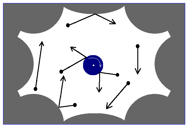
Figure 2. Example of a mechanical system that motivated the present study: Particles in a domain $\Gamma$ (white) are scattered as they are reflected off $\partial\Gamma$, and energy is exchanged when a particle collides with the rotating disk (blue) nailed down at the center of the domain.

Choosing $R=\eta=1$ leads to the especially simple equations

(1.1) $$v_{n}^{\prime}\ =\ -v_{n}\ ,\qquad v_{t}^{\prime}\ =\ \omega\ ,\qquad\omega^{\prime}\ =\ v_{t}\ .$$

For simplicity, we will work with these special parameters, though conceptually it makes no difference in the present study.

Connection to stochastic model

Though easy to describe, an analysis of the mechanical model above is considerably outside of the reach of current dynamical systems techniques. Thus we seek to simplify the model while retaining its essential characteristics, including the way in which energy is transferred among particles. By “forgetting” the precise locations of particles in the cell and their directions of travel, as well as the direction of rotation of the disk, we turn the deterministic dynamical system above into a Markov process. Specifically, the times to energy exchange for a particle are determined by exponential distributions with mean $x^{-1/2}$ where $x$ is the instantaneous kinetic energy of the particle, and the repartitioning of energy at exchanges are as in (1.1) assuming random angles of incidence. Details are given in Sect. 1.2.

We provide below some heuristic justification for the memory loss and interaction rates proposed in the last paragraph:

First we explain the rationale behind neglecting precise locations within a cell. Billard systems on domains with concave boundaries (or scatterers) are well known to exhibit chaotic, or hyperbolic, behavior [40, 6]. Hyperbolicity here refers to exponential divergence of nearby orbits, a property that leads to rapid loss of memory of trajectory history. By taking the rotating disk in our model to be relatively small, between energy exchanges a typical particle trajectory is reflected many times as it bounces off the walls of the domain. (Adding more scatterers in $\Gamma\setminus D$ as was done in [29] will further enhance mixing.) As our system is a hyperbolic billiard between collisions with the rotating disk, the rapid loss of memory gives justification for neglecting precise locations within a cell.

Next we explain the use of exponential random variables to describe the times between collisions. Another well known fact for strongly hyperbolic systems including billiards is that for points randomly distributed in a specific region, return times to this region have exponentially small tails [47]. Thus for particles that emerge from an energy exchange with a fixed energy but randomly distributed otherwise in terms of location and angle, we can expect the times to their next collision with the disk to have an exponentially small tail.

Finally, fixing initial location and direction of travel, the time for a particle to reach a pre-specified region is proportional to its speed; that is the rationale for assuming mean collision time is proportional to $x^{-1/2}$.

For another confirmation of the close connection between the stochastic model in Sect. 1.2 and the mechanical model above, notice that modulo constants their invariant measures coincide; see the remark following Proposition 1.

1.2. Precise description of stochastic model

The stochastic model considered in the rest of this paper is a time-homogeneous Markov jump process $\mathbf{x}_{t},t\geq 0$, with

$$\mathbf{x}_{t}=(x^{1}_{t},\dots,x^{m}_{t},y_{t})\ .$$

Here $m$ is a fixed positive integer, $x^{1}_{t},\dots,x^{m}_{t}$ are the energies of the $m$ particles at time $t$, and $y_{t}$ is the energy of the disk, which we regard from here on as an abstract “energy tank”. As the domain is assumed to be closed, total energy remains constant in time, i.e., there exists a constant $\bar{E}>0$ such that $\sum_{i}x^{i}_{t}+y_{t}=\bar{E}$ for all $t\geq 0$. Thus the state space of $\mathbf{x}_{t}$ is the open $(m+1)$-dimensional simplex

$${\bf\Delta}={\bf\Delta}^{m+1}(\bar{E})=\left\{(x^{1},\cdots,x^{m},y)\in\mathbb{R}^{m+1}_{+}\,|\,y+\sum_{i=1}^{m}x^{i}=\bar{E}\right\}\,.$$

As in the mechanical model in Sect. 1.1, the particles in this system do not interact directly with one another. Instead, they interact via the energy tank, which symbolizes the “environment” within the domain, and it is these particle-tank interactions that give rise to the jumps in the process. The rules of interaction are as follows: Particle $i$ carries a clock that rings at an exponential rate equal to $\sqrt{x^{i}_{t}}$; notice that this rate changes each time the particle acquires a new energy. The clocks carried by different particles are independent of one another and of history. When its clock rings, a particle exchanges energy with the tank according to the following rule: Suppose the clock of particle $i$ rings at time $t$, and let $\mathbf{x}_{t^{+}}=(x^{1}_{t^{+}},x^{2}_{t^{+}},\dots,x^{m}_{t^{+}},y_{t^{+}})$ denote the state immediately following the interaction at time $t$. Then assuming that the angles of incidence are uniformly distributed, the rules for updating, i.e. (1.1), translate into

(1.2) $$x^{i}_{t^{+}}=y_{t}+(1-u^{2})x^{i}_{t},\quad y_{t^{+}}=u^{2}x^{i}_{t},\qquad\mbox{and }\quad x^{j}_{t^{+}}=x^{j}_{t}\quad\mbox{ for }j\neq i\ ,$$

where $u\in(0,1)$ is a uniform random variable. For a detailed calculation, see [29].

The transition probabilities above together with an initial condition $\mathbf{x}_{0}$ defines the Markov process $\mathbf{x}_{t}$. The notation $\mathbf{x}_{t}=(x^{1}_{t},\dots,x^{m}_{t},y_{t})$ is used throughout; in particular, $x^{i}$ is used exclusively to denote the energy of the $i$th particle, not the $i$th power of $x$.

We fix also the following notation: For $t\geq 0$ and $\mathbf{x}\in\mathbf{\Delta}$, let $P^{t}(\mathbf{x},\cdot)$ be the transition probabilities of the process $\mathbf{x}_{t}$. That is to say, $P^{t}(\mathbf{x},\cdot)$ is the Borel probability distribution on $\mathbf{\Delta}$ describing the possible states of the system $t$ units of time later given that its initial condition is $\mathbf{x}$. To simplify notation, we use the same notation for the left and right operators generated by $P^{t}$:

$$(P^{t}\xi)(\mathbf{x})=\int_{\mathbf{\Delta}}P^{t}(\mathbf{x},\mathrm{d}\mathbf{y})\xi(\mathbf{y})$$

for a measurable function $\xi$ on $\mathbf{\Delta}$, and

$$(\mu P^{t})(A)=\int_{\mathbf{\Delta}}P^{t}(\mathbf{x},A)\mu(\mathrm{d}\mathbf{x})$$

for a probability measure $\mu$ on $\mathbf{\Delta}$. Finally we say $\mu$ is an invariant measure for the process $\mathbf{x}_{t}$ if $\mu P^{t}=\mu$ for all $t>0$.

1.3. Statement of results

Proposition 1. The probability measure $\pi$ with density

$$\rho(x^{1},\cdots,x^{m},y)=\frac{1}{Z}\ y^{-1/2}$$

where $Z$ is a normalizing constant is an invariant measure for the process $\mathbf{x}_{t}$.

By the change of variables $x=|\mathbf{v}_{i}|^{2}$ and $y=\tilde{\omega}^{2}$, one sees that $\pi$ coincides with Liouville measure on a fixed energy shell for a Hamiltonian system with $H=|\mathbf{v}_{i}|^{2}+\tilde{\omega}^{2}$. Here $\mathbf{v}_{i}$ is the velocity of the $i$th particle, and $\tilde{\omega}$ is the angular velocity of the rotating disk.

Theorem 1 (Uniqueness of invariant measure). The measure $\pi$ in Proposition 1 is the unique invariant probability for $\mathbf{x}_{t}$; hence it is ergodic.

Theorem 2 (Speed of convergence to equilibrium). For every $\mathbf{x}\in\mathbf{\Delta}$ and $\gamma>0$,

$$\lim_{t\rightarrow\infty}\ t^{2-\gamma}\ \|P^{t}(\mathbf{x},\cdot)-\pi\|_{TV}=0$$

where $\|\cdot\|_{TV}$ is the total variational norm.

Theorem 2 is in fact deduced from Theorem 3 below. For ${\delta}>0$, let $\mathcal{M}_{\delta}$ be the collection of probability measures $\mu$ on $\mathbf{\Delta}$ such that

$$\int_{\bf\Delta}\left(\sum_{k=1}^{m}(x^{k})^{2{\delta}-1}+y^{{\delta}-\frac{1}{2}}\right)\mu(\mathrm{d}\mathbf{x})\ <\ \infty\ .$$

Theorem 3 (Polynomial contraction of Markov operator). For any $\gamma>0$ and $\mu,\nu\in\mathcal{M}_{\gamma/8}$,

$$\lim_{t\rightarrow\infty}\ t^{2-\gamma}\ \|\mu P^{t}-\nu P^{t}\|_{TV}=0\,.$$

The following simple argument shows that the bound in Theorem 3 is tight: Consider, for example, two initial distributions $\mu$ and $\nu$ that differ by a positive amount when restricted to the set $B_{\epsilon}:=\{x^{i}<\epsilon\}$ for some fixed $i$. For definiteness, let us assume that for all small enough $\epsilon$, $\mu|_{B_{\epsilon}}\leq c\pi|_{B_{\epsilon}}$ and $\nu|_{B_{\epsilon}}\geq c^{\prime}\pi|_{B_{\epsilon}}$ for some $c<1<c^{\prime}$. Since $\pi(B_{\epsilon})\propto\epsilon$, $x^{i}<\frac{1}{t^{2}}$ implies that the probability with respect to $\pi$ of the $i$th clock ringing before time $t$ is $<1-e^{-1}$. It follows that

$$\|\mu P^{t}-\nu P^{t}\|_{TV}\geq\|(\mu P^{t}-\nu P^{t})|_{\{x^{i}<\frac{1}{t^{2}}\}}\|_{TV}\geq\mbox{ constant}\cdot\frac{1}{t^{2}}\ .$$

Another corollary of Theorem 3 is the rate of decay of time correlations.

Theorem 4 (Polynomial correlation decay). For any $\gamma>0$ and $\mu\in\mathcal{M}_{\gamma/8}$, let $\xi$ and $\zeta\in L^{\infty}(\mathbf{\Delta})$. Then

$$\left|\int_{\mathbf{\Delta}}(P^{t}\zeta)(\mathbf{x})\xi(\mathbf{x})\mu(\mathrm{d}\mathbf{x})-\int_{\mathbf{\Delta}}(P^{t}\zeta)(\mathbf{x})\mu(\mathrm{d}\mathbf{x})\int_{\mathbf{\Delta}}\xi(\mathbf{x})\mu(\mathrm{d}\mathbf{x})\right|\ =\ o\left(\frac{1}{t^{2-\gamma}}\right)$$

as $t\to\infty$.

The next result is another consequence of Theorem 3.

Theorem 5 (Central limit theorem). Let $f:\mathbf{\Delta}\rightarrow\mathbb{R}$ be a Borel function that is uniformly bounded $\pi$-a.s. For any $\delta>0$, let $\{f^{\delta}_{n}\}_{n=1}^{\infty}=\{f(\mathbf{x}_{0}),f(\mathbf{x}_{\delta}),\cdots,f(\mathbf{x}_{n\delta}),\cdots\}$ be a sequence of observables, and define

$$\bar{f}=\frac{1}{n}\sum_{i=0}^{n}f^{\delta}_{n}\,.$$

Then for any initial distribution $\mathbf{x}_{0}$,

$$\sqrt{n}(\bar{f}-\mathbb{E}_{\pi}f)\xrightarrow{d}N(0,\sigma^{2}_{f})\qquad\mbox{ as }n\rightarrow\infty\ ,$$

provided

$$\sigma_{f}^{2}:=\mathrm{var}_{\pi}\{f(\mathbf{x}_{0})\}+2\sum_{i=1}^{\infty}\mathrm{cov}\{f(\mathbf{x}_{0}),f(\mathbf{x}_{i\delta})\}<\infty\,.$$

2. Construction of Lyapunov function

Let $\mathbf{\Delta}$ be as in Sect. 1.2. For $\alpha<\frac{1}{2}$, we define $V=V_{\alpha}:\mathbf{\Delta}\to\mathbb{R}^{+}$ by

$$V(\mathbf{x})=V_{\alpha}(\mathbf{x})=\sum_{i=1}^{m}(x^{i})^{-2\alpha}+y^{-\alpha}\ .$$

Our main technical result is the following:

Theorem 2.1.

For $\alpha<\frac{1}{2}$ close enough to $\frac{1}{2}$ and $h>0$ small enough, there exist $c_{0},M>0$ depending on $\alpha$ and $h$ such that for $V=V_{\alpha}$ and $\beta=1-(4\alpha)^{-1}$,

$$(P^{h}V)(\mathbf{x})-V(\mathbf{x})\leq-c_{0}V(\mathbf{x})^{\beta}$$

for every $\mathbf{x}\in\{V>M\}$.

The motivation for this choice of Lyapunov function is as follows. As noted in the Introduction, low energy particles are our main concern, for they are not expected to interact for a long time, and that slows down the mixing process. For this reason, a desirable Lyapunov function should satisfy $V(\mathbf{x})\rightarrow\infty$ as $\mathbf{x}\rightarrow\partial\mathbf{\Delta}$. We explain heuristically why one may expect something along the lines of $P^{h}V-V\sim-hV^{1/2}$, corresponding to $\alpha,\beta\approx 2$: Assume $x^{1}\ll 1$ is the smallest particle energy. Then $V(\mathbf{x})\sim(x^{1})^{-1}$. If the clock of particle $1$ rings on the time interval $[0,h)$ and $y$ is “large”, then the expected drop of $V(\mathbf{x})$ following an interaction is $\sim(x^{1})^{-1}\sim V(\mathbf{x})$. But the probability that the clock of particle $1$ will ring exactly once before time $h$ is $\sim h\sqrt{x^{1}}$. This means the expected drop of $V(\mathbf{x})$ is $\sim h(x^{1})^{-1/2}\sim hV^{1/2}$.

It is convenient to use the following equivalent description of $\Phi_{t}$: Starting from $t=0$, a clock rings at time $\tau_{1}$ where $\tau_{1}$ is an exponential random variable with mean $(\sum_{i=1}^{m}\sqrt{x^{i}_{0}})^{-1}$. When this clock rings, energy exchange takes place between exactly one particle and the tank, and the probability that particle $i$ is chosen is

$$\frac{\sqrt{x^{i}_{0}}}{\sum_{i=1}^{m}\sqrt{x^{i}_{0}}}\,.$$

The rule of energy redistribution is determined by equation (1.2) as before, and this process is repeated, i.e., at time $\tau_{2}$, an exponential random variable with mean $\left(\sum_{i=1}^{m}\sqrt{x^{i}_{\tau_{1}^{+}}}\right)^{-1}$, the clock rings again, and so on.

We begin with the following technical estimate:

Lemma 2.2.

There exist constants $\epsilon_{0}>0$ and $c^{*}>0$ such that

$$\mathbb{E}[V(\mathbf{x}_{\tau_{1}^{+}})\,|\,\mathbf{x}_{0}]\leq V(\mathbf{x}_{0})-\frac{c^{*}}{\sum_{i=1}^{m}\sqrt{x^{i}_{0}}}V(\mathbf{x}_{0})^{\beta}$$

for every $\mathbf{x}_{0}\in B$, where

$$B=\left\{\mathbf{x}\in\mathbf{\Delta}\,|\,y<\epsilon_{0},\ \mbox{ or }\ x^{i}<4^{-\frac{1}{2\alpha}}\epsilon_{0}\ \mbox{ for some }\ i\in\{1,\dots,m\}\right\}\ .$$

Proof.

By definition,

$$\mathbb{E}[V(\mathbf{x}_{\tau_{1}^{+}})\,|\,\mathbf{x}_{0}]\ =\ V(\mathbf{x}_{0})+\frac{1}{\sum_{i=1}^{m}\sqrt{x^{i}_{0}}}\sum_{i=1}^{m}Q_{i}$$

where

$$Q_{i}\ =\ \sqrt{x^{i}_{0}}\left\{\int_{0}^{1}\left[(x_{0}^{i}(1-u^{2})+y_{0})^{-2\alpha}+(x_{0}^{i}u^{2})^{-\alpha}\right]\mathrm{d}u-\left[(x_{0}^{i})^{-2\alpha}+y_{0}^{-\alpha}\right]\right\}\ ,$$

i.e., we need to show $\sum Q_{i}\leq-c^{*}V(\mathbf{x}_{0})^{\beta}$ for some $c^{*}>0$. In the rest of the proof, we will omit the subscript $0$ in $\mathbf{x}_{0},\ x^{i}_{0}$ and $y_{0}$, and write

$$C_{1}=\int_{0}^{1}(1-u^{2})^{-2\alpha}\mathrm{d}u\qquad\mbox{ and }\qquad C_{2}=\int_{0}^{1}u^{-2\alpha}\mathrm{d}u,$$

noting that $C_{1},C_{2}<\infty$ for $\alpha<\frac{1}{2}$. We will use many times the bound

(2.1) $$Q_{i}\ \leq\ \sqrt{x^{i}}\left\{\min\{C_{1}(x^{i})^{-2\alpha},y^{-2\alpha}\}+C_{2}(x^{i})^{-\alpha}-(x^{i})^{-2\alpha}-y^{-\alpha}\right\}\ .$$

Without loss of generality assume

$$x^{1}=\min_{1\leq i\leq m}x^{i}\ .$$

Let $0<\epsilon_{0}\ll\epsilon_{1}\ll\bar{E}$ be two small numbers to be determined. We decompose $B$, the neighborhood of $\partial{\bf\Delta}$ in the statement of the lemma, into three regions (see Fig 3) and analyze each one as follows:

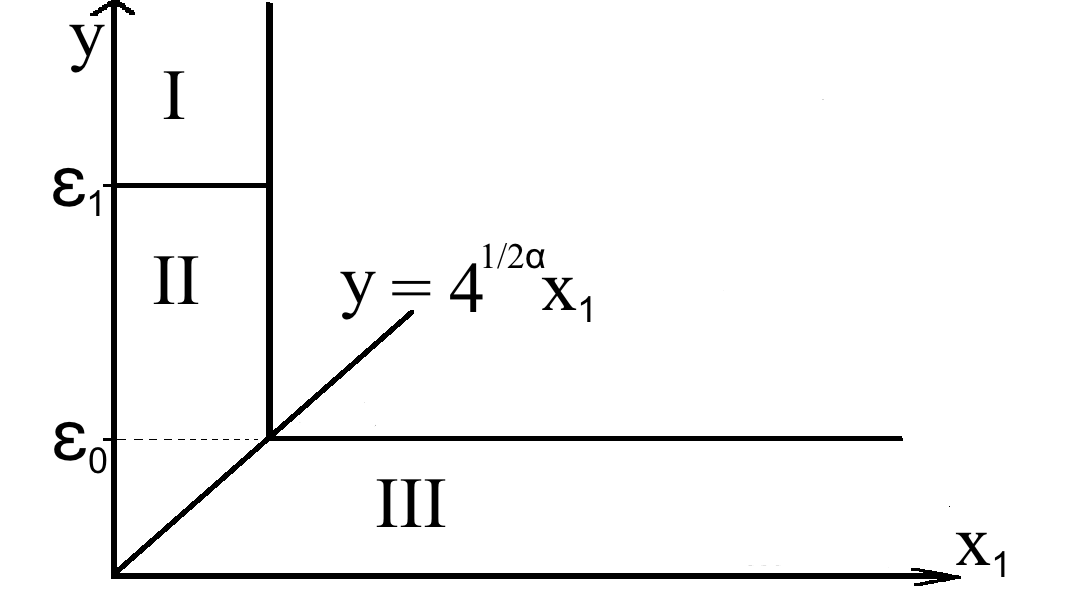
Figure 3. Decomposition of neighborhood of $\partial\mathbf{\Delta}$

Region I.  $4^{\frac{1}{2\alpha}}x^{1}<\epsilon_{0},\ y\geq\epsilon_{1}$

With regard to lowering $V$, we clearly have the most to gain if particle 1 interacts with the tank: Applying (2.1) to $x^{1}$ and substituting in $y\geq\epsilon_{1}$, we obtain

$$Q_{1} \leq \sqrt{x^{1}}\cdot\left\{(\epsilon_{1})^{-2\alpha}+C_{2}(x^{1})^{-\alpha}-(x^{1})^{-2\alpha}\right\}\ .$$

Using $4^{\frac{1}{2\alpha}}x^{1}<\epsilon_{0}\ll\epsilon_{1}$, we see that the third term dominates. Hence

$$Q_{1}\leq-\frac{1}{2}(x^{1})^{-2\alpha+\frac{1}{2}}\ .$$

For $i\neq 1$, we consider separately the following two cases: For $x^{i}<\frac{1}{2}\epsilon_{1}<\frac{1}{2}y$, we have

(2.2) $$Q_{i}\ \leq\ \sqrt{x^{i}}\left\{(2x^{i})^{-2\alpha}+C_{2}(x^{i})^{-\alpha}-(x^{i})^{-2\alpha}\right\}\ ,$$

which is $<0$ since the last term dominates. If $x^{i}\geq\frac{1}{2}\epsilon_{1}$, then from (2.1) we obtain

$$Q_{i}\ \leq\ \sqrt{x^{i}}\{C_{1}(x^{i})^{-2\alpha}+C_{2}(x^{i})^{-\alpha}\}\leq C^{\prime}(\epsilon_{1})^{-2\alpha+\frac{1}{2}}$$

for some $C^{\prime}$ independent of $\epsilon_{0}$ or $\epsilon_{1}$. Notice that we have used $\frac{1}{2}-2\alpha<0$, or $\alpha>\frac{1}{4}$.

Altogether, we have shown, using $\epsilon_{0}\ll\epsilon_{1}\ll 1$, that

$$\sum_{i=1}^{m}Q_{i} \leq -\frac{1}{2}(x^{1})^{-2\alpha+\frac{1}{2}}+(m-1)C^{\prime}(\epsilon_{1})^{-2\alpha+\frac{1}{2}}\leq-\frac{1}{3}(x^{1})^{-2\alpha+\frac{1}{2}}\ .$$

It follows from $V(\mathbf{x})\leq(m+1)(x^{1})^{-2\alpha}$ that this is $\leq-\frac{1}{3(m+1)}V(\mathbf{x})^{\beta}$.

Region II.  $4^{\frac{1}{2\alpha}}x^{1}<\epsilon_{0},\ 4^{\frac{1}{2\alpha}}x^{1}<y<\epsilon_{1}$

For $i=1$, applying (2.1) and using $y>4^{\frac{1}{2\alpha}}x^{1}$, we obtain

$$Q_{1} \leq \sqrt{x^{1}}\left\{(4^{\frac{1}{2\alpha}}x^{1})^{-2\alpha}+C_{2}(x^{1})^{-\alpha}-(x^{1})^{-2\alpha}\right\}\leq-\frac{1}{2}(x^{1})^{-2\alpha+\frac{1}{2}}\ .$$

For $i\neq 1$, if $x^{i}<\frac{1}{2}y$, then the situation is as in (2.2), and $Q_{i}<0$. The case where $x^{i}\geq\frac{1}{2}y$ is one of the more delicate: Applying (2.1), we obtain

$$Q_{i}\ \leq\ C^{\prime\prime}x^{-2\alpha+\frac{1}{2}}-\sqrt{x}y^{-\alpha}\ \leq C^{\prime\prime\prime}y^{-2\alpha+\frac{1}{2}}-\sqrt{x}y^{-\alpha}\ .$$

Without loss of generality, assume $x^{2},\cdots,x^{k}\geq\frac{1}{2}y$, and $x^{j}<\frac{1}{2}y$ for all $j>k$. Then $\max\{x^{2},\dots,x^{k}\}>\frac{\bar{E}}{2m}$. Therefore

$$\sum_{i=2}^{k}Q_{i} \leq (k-1)C^{\prime\prime\prime}y^{-2\alpha+\frac{1}{2}}-\left(\sum_{i=2}^{k}\sqrt{x^{i}}\right)y^{-\alpha}$$

$$\leq y^{-\alpha}\left[mC^{\prime\prime\prime}y^{-\alpha+\frac{1}{2}}-\sqrt{\frac{\bar{E}}{2m}}\right]\ .$$

As $y<\epsilon_{1}$ and $\alpha<\frac{1}{2}$, the quantity in square brackets is $<0$ provided $\epsilon_{1}$ is sufficiently small.

Thus arguing as in Region I, we have shown that

$$\sum_{i=1}^{m}Q_{i}\ \leq\ -\frac{1}{2}(x^{1})^{-2\alpha+\frac{1}{2}}\ <\ -\frac{1}{2(m+1)}V(\mathbf{x})^{\beta}\ .$$

Region III.  $4^{\frac{1}{2\alpha}}x^{1}\geq y,\ y<\epsilon_{0}$

Since $x^{i}\geq x^{1}\geq 4^{-\frac{1}{2\alpha}}y$ for all $i$, a calculation analogous to that in Region II gives

$$\sum_{i=1}^{m}Q_{i}\ \leq\ y^{-\alpha}\left[mC^{\prime\prime\prime\prime}y^{-\alpha+\frac{1}{2}}-\sqrt{\frac{\bar{E}}{2m}}\right]\ <\ -\frac{1}{2}\sqrt{\frac{\bar{E}}{2m}}\ y^{-\alpha}$$

provided $\epsilon_{0}$ is small enough. Since $V(\mathbf{x})\leq m(x^{1})^{-2\alpha}+y^{-\alpha}\leq(4m+1)y^{-2\alpha}$, it follows that

$$\sum_{i=1}^{m}Q_{i}\leq-\frac{1}{2}\sqrt{\frac{\bar{E}}{2m}}\cdot\frac{1}{\sqrt{4m+1}}V(\mathbf{x})^{\frac{1}{2}}\leq-\frac{1}{2}\sqrt{\frac{\bar{E}}{2m}}\cdot\frac{1}{\sqrt{4m+1}}V(\mathbf{x})^{\beta}$$

since $\beta<\frac{1}{2}$.

The assertion is proved since it holds for $\mathbf{x}_{0}$ in all three regions of $B$. ∎

Proof of Theorem 2.1.

Let $\tau_{1}<\tau_{2}<\dots$ be the times of clock rings as defined in the paragraph preceding the statement of Lemma 2.2, and let $B$ be the neighborhood of $\partial\bf\Delta$ in Lemma 2.2. Letting $\tau_{0}=0$, we have shown that for any $n\geq 0$, if $\mathbf{x}_{\tau_{n}^{+}}\in B$, then

(2.3) $$\mathbb{E}[V(\mathbf{x}_{\tau_{n+1}^{+}})\,|\,\mathbf{x}_{\tau_{n}^{+}}]\ \leq\ V(\mathbf{x}_{\tau_{n}^{+}})\ -\ \frac{c^{*}}{\sum_{i=1}^{m}\sqrt{x^{i}_{\tau_{n}^{+}}}}\ V(\mathbf{x}_{\tau_{n}^{+}})^{\beta}\ .$$

For $\mathbf{x}_{\tau_{n}^{+}}\not\in B$, we will use the bound

(2.4) $$\mathbb{E}[V(\mathbf{x}_{\tau_{n+1}^{+}})\,|\,\mathbf{x}_{\tau_{n}^{+}}]\ \leq\ M_{0}+M_{1}$$

where

$$M_{0}=\sup_{\mathbf{x}\in{\bf\Delta}\setminus B}V(\mathbf{x})\quad\mbox{ and }\quad M_{1}=\sup_{\mathbf{x}\in{\bf\Delta}\setminus B}\frac{1}{\sum_{i=1}^{m}\sqrt{x^{i}}}\sum_{i=1}^{m}Q_{i}(\mathbf{x})\ .$$

It is easy to check that $M_{0},M_{1}<\infty$.

We now use these estimates to deduce a bound for $P^{h}V$ for fixed $h>0$. Let $S=\inf\{n,\tau_{n}>h\}$, and define $\hat{\tau}_{n}=\min\{\tau_{n},\tau_{S-1}\}$. Then

$$P^{h}V(\mathbf{x})=\lim_{n\to\infty}\mathbb{E}[V(\mathbf{x}_{\hat{\tau}_{n}^{+}}){\bf 1}_{S\leq n+1}\,|\,\mathbf{x}_{0}=\mathbf{x}]\leq\lim_{n\to\infty}\mathbb{E}[V(\mathbf{x}_{\hat{\tau}_{n}^{+}})\,|\,\mathbf{x}_{0}=\mathbf{x}]\ .$$

We will prove a uniform bound for $\mathbb{E}[V(\mathbf{x}_{\hat{\tau}_{n}^{+}})\,|\,\mathbf{x}_{0}=\mathbf{x}]$ for all $n\geq 1$.

First, assuming the worse of (2.3) and (2.4), we have

(2.5) $$\mathbb{E}[V(\mathbf{x}_{\tau_{n+1}^{+}})\,|\,\tau_{n+1}\leq h]\ \leq\ E[V(\mathbf{x}_{\tau_{n}^{+}})\,|\,\tau_{n+1}\leq h]+M_{0}+M_{1}$$

for every $n\geq 0$. Notice that conditioning on $\tau_{n+1}\leq h$ does not affect the bounds in (2.3) and (2.4) because given $\mathbf{x}_{\tau_{n}^{+}}$, $\mathbf{x}_{\tau_{n+1}^{+}}$ is independent of $\tau_{n+1}-\tau_{n}$. Second, as $\sum_{i=1}^{m}\sqrt{x^{i}}\leq\sqrt{m\bar{E}}$ for all $\mathbf{x}\in\bf\Delta$, we have, for every $\mathbf{x}_{\tau_{n}^{+}}\in\bf\Delta$,

$$\mathbb{P}[\tau_{n+1}\leq h\,|\,\mathbf{x}_{\tau_{n}^{+}},\tau_{n}\leq h]\leq\left(1-e^{-h\sqrt{m\bar{E}}}\right)\ \mathbb{P}[\tau_{n}\leq h]\ ,$$

so that inductively,

(2.6) $$\mathbb{P}[\tau_{n+1}\leq h\,|\,\mathbf{x}_{0}]\leq\left(1-e^{-h\sqrt{m\bar{E}}}\right)^{n+1}\qquad\mbox{ for }\quad n\geq 0\ .$$

The estimates (2.5) and (2.6) together imply the following: Given $\mathbf{x}_{0}=\mathbf{x}$,

$$\mathbb{E}[V(\mathbf{x}_{\hat{\tau}_{n+1}^{+}})]$$

$$= \mathbb{E}[V(\mathbf{x}_{\hat{\tau}_{n+1}^{+}})\,|\,\tau_{n+1}>h]\cdot\mathbb{P}[\tau_{n+1}>h]+\mathbb{E}[V(\mathbf{x}_{\hat{\tau}_{n+1}^{+}})\,|\,\tau_{n+1}\leq h]\cdot\mathbb{P}[\tau_{n+1}\leq h]$$

$$\leq \mathbb{E}[V(\mathbf{x}_{\hat{\tau}_{n}^{+}})\,|\,\tau_{n+1}>h]\cdot\mathbb{P}[\tau_{n+1}>h]$$

$$\hskip 28.45274pt+\left(\mathbb{E}[V(\mathbf{x}_{\hat{\tau}_{n}^{+}})\,|\,\tau_{n+1}\leq h]+M_{0}+M_{1}\right)\cdot\mathbb{P}[\tau_{n+1}\leq h]$$

$$\leq \mathbb{E}[V(\mathbf{x}_{\hat{\tau}_{n}^{+}})]+(M_{0}+M_{1})(1-e^{-h\sqrt{m\bar{E}}})^{n+1}\ .$$

Summing over $n$, this gives

$$P^{h}V(\mathbf{x})\leq\mathbb{E}[V(\mathbf{x}_{\hat{\tau}_{1}^{+}})\,|\,\mathbf{x}_{0}=\mathbf{x}]+\frac{M_{0}+M_{1}}{e^{-h\sqrt{m\bar{E}}}}\,.$$

Let $h>0$ be small enough so that for all $\mathbf{x}\in\bf\Delta$,

$$\mathbb{P}[\tau_{1}\leq h\,|\,\mathbf{x}_{0}=\mathbf{x}]=1-e^{-h\sum_{i=1}^{m}\sqrt{x^{i}}}>\frac{h}{2}\sum_{i=1}^{m}\sqrt{x^{i}}\ .$$

This is the only condition we impose on $h$.

We choose $M^{\prime}$ large enough so that $\{V>M^{\prime}\}\subset B$, and consider $\mathbf{x}_{0}\in\{V>M^{\prime}\}$. Noting again that $\mathbb{E}[V(\mathbf{x}_{{\tau}_{1}^{+}})]$ is independent of $\tau_{1}$, we have, by Lemma 2.2,

$$\mathbb{E}[V(\mathbf{x}_{\hat{\tau}_{1}^{+}})] = \mathbb{E}[V(\mathbf{x}_{\tau_{1}^{+}})\,|\,\tau_{1}\leq h]\cdot\mathbb{P}[\tau_{1}\leq h]+V(\mathbf{x}_{0})\cdot\mathbb{P}[\tau_{1}>h]$$

$$\leq \left(V(\mathbf{x}_{0})-\frac{c^{*}}{\sum\sqrt{x^{i}}}V(\mathbf{x}_{0})^{\beta}\right)\cdot\mathbb{P}[\tau_{1}\leq h]+V(\mathbf{x}_{0})\cdot\mathbb{P}[\tau_{1}>h]$$

$$\leq V(\mathbf{x}_{0})-c^{*}\frac{h}{2}V(\mathbf{x}_{0})^{\beta}\ .$$

This gives

$$P^{h}V(\mathbf{x})\leq V(\mathbf{x})-c^{*}\frac{h}{2}V(\mathbf{x})^{\beta}+(M_{0}+M_{1})e^{h\sqrt{m\bar{E}}}\ .$$

To complete the proof of Theorem 2.1, it suffices to replace $M^{\prime}$ by a large enough number $M$ so that for $\mathbf{x}\in\{V>M\}$, the constant $(M_{0}+M_{1})e^{h\sqrt{m\bar{E}}}$ is absorbed into $c_{0}V(\mathbf{x})^{\beta}$ for $c_{0}=c^{*}\frac{h}{4}$. ∎

We record for later use the following fact that follows from the proof above:

Corollary 2.3.

$$\sup_{\mathbf{x}\not\in B}P^{h}V(\mathbf{x})\ <\ \infty$$

3. Completing the proofs

After some preliminaries in Sect. 3.1, we proceed to the main task of this section, the deduction of Theorem 3 from the Lyapunov function introduced. Two proofs are given, one in Sects. 3.2 and 3.3 and the other in Sect. 3.4. Proofs of Theorems 2, 4 and 5 follow quickly once Theorem 3 is proved.

3.1. Existence and uniqueness of invariant measure

Proof of Proposition 1.

Let $\pi$ be the probability measure with density $\rho(x^{1},\dots,x^{m},y)$ $=\frac{1}{Z}y^{-1/2}$. To prove $\pi=\pi P^{\xi}$ for $\xi\ll 1$, it suffices to fix an arbitrary state $\mathbf{\bar{x}}=(\bar{x}^{1},\cdots,\bar{x}^{m},\bar{y})\in\mathbf{\Delta}$, let

$$D=D(\mathbf{\bar{x}},\epsilon)=\{\mathbf{x}\in\mathbf{\Delta}\,|\,|x^{i}-\bar{x}^{i}|,|y-\bar{y}|<\epsilon\ \forall i\}$$

for $\epsilon>0$ arbitrarily small, and show that

$$\mathbb{P}_{\pi}[\mathbf{x}_{0}\in D,E]=\mathbb{P}_{\pi}[\mathbf{x}_{\xi}\in D,E]+O(\xi^{2})$$

where $E$ is the event that exactly one interaction takes place on the interval $(0,\xi)$. Clearly,

$$\mathbb{P}_{\pi}[\mathbf{x}_{0}\in{D},E]=\xi(2\epsilon)^{m}\left(\sum_{i=1}^{m}\sqrt{\bar{x}^{i}}\right)\cdot Z^{-1}\bar{y}^{-1/2}+O(\xi^{2}\epsilon^{m}+\xi\epsilon^{m+1})\,.$$

The estimation of $\mathbb{P}_{\pi}[\mathbf{x}_{\xi}\in D,E]$ requires a straightforward computation identical to that in Lemma 6.6 of [29]. ∎

To prove uniqueness, we prove Doeblin’s condition on a subset of $\bf\Delta$, which for convenience we take to be a set of “active states” of the form

$$A_{\epsilon}:=\{\mathbf{x}\in\mathbf{\Delta}\,|\,x^{i},y\geq\epsilon\}$$

for some $\epsilon>0$. For $S\subset\bf\Delta$, let $U_{S}$ denote the uniform probability measure on $S$.

Proposition 3.1.

For any $t>0$ and $\epsilon>0$, there exists a constant $\eta=\eta(\epsilon,t)$ such that for every $\mathbf{x}\in A=A_{\epsilon}$,

$$P^{t}(\mathbf{x},\cdot)\geq\eta U_{A}(\cdot)\ .$$

Proof.

We cover $A$ with finitely many sets of the form $D=D(\mathbf{\bar{x}},\xi)$ where $D(\mathbf{\bar{x}},\xi)$ is as defined in the proof of Proposition 1 with the property that dist$(D,\partial{\bf\Delta})>\frac{4\epsilon}{5}$. It suffices to show that given any $t>0$, there exists $\eta>0$ such that for every $\mathbf{x}\in A$, $P^{t}(\mathbf{x},\cdot)\geq\eta U_{D}(\cdot)$ for all the $D$ in this cover. There are many ways to arrive at this outcome; below we describe one possible scenario.

Let $\mathbf{x}$ and $D$ be fixed. There will be two rounds of interactions. The first round, which takes place on the time interval $(0,\frac{t}{2})$, will result in most of the energy collecting in the tank; and in the second round, which takes place on $(\frac{t}{2},t)$, energy is redistributed according to $D$. In more detail, starting from $\mathbf{x}$, the first round consists of particle 1 interacting twice with the tank in quick succession, followed by particle 2, and so on through particle $m$, with no other interactions besides these. For each $i$, the goal of the second interaction is to result in $x^{i}_{\frac{t}{2}}\in(\frac{2\epsilon}{5},\frac{3\epsilon}{5})$. This requires two interactions to achieve because after the first interaction, $x^{i}_{s^{+}}\geq y_{s}$ (see (1.2)), and tank energy prior to interaction with each particle is $\geq\epsilon$. In the second round, each particle interacts twice with the tank as before, resulting in $x^{i}_{t}\in[\bar{x}^{i}-\xi,\bar{x}^{i}+\xi]$ uniformly distributed and independent of $x^{j}_{t}$ for $j=1,2,\dots,i-1$.

We leave it to the reader to check that the scenario above occurs with probability $\eta>0$ independent of $\mathbf{x}$ provided $\mathbf{x}\in A$. ∎

Proof of Theorem 1.

Let $A=A_{\epsilon}$ and $t$ be as above. It is obvious that for any $\mathbf{x}\in{\bf\Delta}$, $P^{t/2}(\mathbf{x},A)>0$. Together with Proposition 3.1, this implies that $P^{t}(\mathbf{x},\cdot)$ has a strictly positive density on all of $A$, and that in turn implies that all $\mathbf{x}\in{\bf\Delta}$ belong in the same ergodic component, equivalently, $\mathbf{x}_{t}$ admits at most one invariant probability measure, which must therefore be $\pi$. ∎

3.2. Review of tools from probability

We recall here some tools that we will use to prove polynomial convergence. As these are very general ideas, we will present them in the context of general Markov chains. Let $\Psi_{n}$ be a (discrete-time) Markov chain on a measurable space $(X,\mathcal{B})$ with transition kernels $\mathcal{P}(x,\cdot)$.

(A) Atoms of Markov chains. A set $\alpha\in\mathcal{B}$ is called an atom if there is a probability measure $\theta$ on $(X,\mathcal{B})$ such that for all $x\in\alpha$, $\mathcal{P}(x,\cdot)=\theta(\cdot)$. Most Markov chains on continuous or uncountable spaces do not possess atoms. We review here a technique introduced in [34] which shows that under quite general conditions for $\Psi_{n}$, one can construct explicitly another chain, $\tilde{\Psi}_{n}$, defined on an enlarged state space $(\tilde{X},\mathcal{\tilde{B}})$, such that $\tilde{\Psi}_{n}$ is an extension of $\Psi_{n}$ and it has an atom.

The relevant condition for $\Psi_{n}$ is that for some set $A_{0}\in\mathcal{B}$, there exists a probability measure $\theta$ and a number $\eta>0$ such that for every $x\in A_{0}$, $\mathcal{P}(x,\cdot)\geq\eta\theta(\cdot)$. Let us call a set $A_{0}$ with this property a special reference set. Assuming the existence of such an $A_{0}$, the splitting technique of [34] is as follows: Let $\tilde{X}=X\cup A_{1}$ (disjoint union) where $A_{1}$ is an identical copy of $A_{0}$, with the obvious extension $\mathcal{\tilde{B}}$ of $\mathcal{B}$ to $\tilde{X}$. First we define the “lift” of a measure $\mu$ on $(X,\mathcal{B})$ to a measure $\mu^{*}$ on $(\tilde{X},\mathcal{\tilde{B}})$:

$$\left\{\begin{array}[]{ll}&\mu^{*}|_{X}=(1-\eta)\ \mu|_{A_{0}}+\mu|_{X\setminus A_{0}}\\ &\mu^{*}|_{A_{1}}=\eta\ \mu|_{A_{0}}\ ,\quad A_{0}\cong A_{1}\mbox{ via the natural identification }.\end{array}\right.$$

The transition kernels $\mathcal{\tilde{P}}(x,\cdot)$ are then given by

$$\left\{\begin{array}[]{cl}\mathcal{\tilde{P}}(x,\cdot)=(\mathcal{P}(x,\cdot))^{*}&x\in X\setminus A_{0}\\ \mathcal{\tilde{P}}(\mathbf{x},\cdot)=[(\mathcal{P}(x,\cdot))^{*}-\eta{\theta^{*}(\cdot)}]/(1-\eta)&x\in A_{0}\\ \mathcal{\tilde{P}}(x,\cdot)={\theta^{*}}(\cdot)&x\in A_{1}\end{array}\right.$$

It is straightforward to check that the chain $\tilde{\Psi}_{n}$ projects to $\Psi_{n}$, meaning $(\mu\mathcal{P})^{*}=\mu^{*}\mathcal{\tilde{P}}$, so that $\|\mu\mathcal{P}^{n}-\nu\mathcal{P}^{n}\|_{\rm TV}\leq\|\mu^{*}\mathcal{\tilde{P}}^{n}-\nu^{*}\mathcal{\tilde{P}}^{n}\|_{\rm TV}$. Finally, $A_{1}$ is an atom for the chain $\tilde{\Psi}_{n}$ — this is the whole point of the construction.

(B) Connection to renewal processes. For $E\in\mathcal{B}$, we let $\tau_{E}$ denote the first passage time to $E$, i.e.,

$$\tau_{E}=\inf\{n>0|\Psi_{n}\in E\}\ .$$

Suppose the chain $\Psi_{n}$ has an atom $\alpha$, and that $\alpha$ is accessible, i.e., $\mathcal{P}_{x}[\tau_{\alpha}<\infty]=1$ for every $x\in X$. Given two initial distributions $\mu$ and $\nu$ on $X$, we wish to bound the rate at which $\|\mu\mathcal{P}^{n}-\lambda\mathcal{P}^{n}\|_{\rm TV}$ tends to $0$ as $n\to\infty$ where $\|\cdot\|_{\rm TV}$ is the total variational norm. One way to proceed is to run two independent copies of the chain with initial distributions $\mu$ and $\nu$ respectively, and perform a coupling at simultaneous returns to the atom $\alpha$. It is well known that if $T$ is the coupling time, then

(3.1) $$\|\mu\mathcal{P}^{n}-\nu\mathcal{P}^{n}\|_{\rm TV}\leq 2\ \mathbb{P}[T>n]\ .$$

The quantities $\mathbb{P}[T>n]$, on the other hand, can be studied via two associated renewal processes as follows:

Let $Y_{0}$ and $Y^{\prime}_{0}$ be independent $\mathbb{N}$-valued random variables having the distributions of $\tau_{\alpha}$, the first passage time to $\alpha$, starting from $\mu$ and $\nu$ respectively, and let $Y_{1},Y_{2},\dots$ and $Y^{\prime}_{1},Y^{\prime}_{2},\dots$ be i.i.d. random variables the distributions of which are equal to that of $\tau_{\alpha}$ starting from $\alpha$. In addition, we assume the return times to $\alpha$ are aperiodic, i.e., $\mathrm{gcd}\{n\geq 1\,|\,\mathbb{P}[Y_{i}=n]>0\}=1$. Then $S_{n}:=\sum_{i=0}^{n}Y_{i}$ and $S^{\prime}_{n}:=\sum_{i=0}^{n}Y^{\prime}_{i}$, $n=0,1,2,\dots$, are renewal processes, and $T$ above is the first simultaneous renewal time, i.e.

$$T=\inf_{n\geq 0}\{S_{k_{1}}=S^{\prime}_{k_{2}}=n\mbox{ for some }k_{1},k_{2}\}\ .$$

The following known result relates the finiteness of the moments of $T$ to the corresponding moments for the distributions of $Y_{0},Y^{\prime}_{0}$ and $Y_{1}$:

Theorem 3.2.

(Theorem 4.2 of [31]) Let $Y_{i}$ and $Y^{\prime}_{i}$ be as above. Suppose that for some $\beta\geq 1$, we have

(3.2) $$\mathbb{E}[Y_{0}^{\beta}],\quad\mathbb{E}[Y_{0}^{\prime\beta}]\quad\mbox{ and }\quad\mathbb{E}[Y_{1}^{\beta}]<\infty\ .$$

Then $\mathbb{E}[T^{\beta}]$ is also finite.

The discussion above implies the following:

Corollary 3.3.

Let $\Psi_{n}$ be a Markov chain on $(X,\mathcal{B})$ with transition kernel $\mathcal{P}$. Suppose $\Psi_{n}$ has an atom $\alpha$ that is accessible and whose return times are aperiodic. Let $\mu$ and $\nu$ be two probability distributions on $X$, and assume that for some $\beta>1$,

$$\mathbb{E}_{\mu}[\tau^{\beta}_{\alpha}],\ \ \mathbb{E}_{\nu}[\tau^{\beta}_{\alpha}]\ \ \mbox{ and }\ \ \mathbb{E}_{\alpha}[\tau^{\beta}_{\alpha}]\ <\infty.$$

Then

$$\lim_{n\to\infty}n^{\beta}\|\mu\mathcal{P}^{n}-\nu\mathcal{P}^{n}\|_{\rm TV}=0\ .$$

The proof is as discussed, together with the following general relation: Let $Z$ be a random variable taking values in $\mathbb{N}$, and let $\beta>1$. Then

(3.3) $$\mathbb{E}[Z^{\beta}]<\infty\ \implies\ \lim_{n\to\infty}n^{\beta}\mathbb{P}[Z>n]=0\ .$$

(C) Lyapunov function and moments of first passage times. The following result, which is sufficient for our purposes, is a simple version of Theorem 3.6 of [22]:

Theorem 3.4.

(Theorem 3.6 of [22]) Let $\Psi_{n}$ be a Markov chain on $(X,\mathcal{B})$ with transition kernel $\mathcal{P}$. We assume that there exist a function $W:X\rightarrow[1,\infty)$, a set $A\in\mathcal{B}$, constants $b,c>0$ and $0\leq\beta<1$ such that

(3.4) $$\mathcal{P}W-W\leq-cW^{\beta}+b\mathbf{1}_{A}\,.$$

Then there is a constant $\hat{c}$ such that for all $x\in X$,

$$\mathbb{E}_{x}\left[\sum_{k=0}^{\tau_{A}-1}(k+1)^{\hat{\beta}-1}\right]\leq\hat{c}W(x)\ ,\qquad\hat{\beta}=(1-\beta)^{-1}\ .$$

Clearly, $\mathbb{E}_{x}[\tau_{A}^{\hat{\beta}}]$ is bounded above by a constant times the expectation above.

The reader may notice that we have omitted some of the hypotheses in Theorem 3.6 of [22] in the statement of Theorem 3.4 above. This is because they are not needed: here we consider only the first passage time to $A$, which can be thought of as a set of the form $\{W\leq{\rm constant}\}$, while [22] considers first passage times to arbitrary sets. We remark also that [22] does not give the rate of convergence to equilibrium we claim; it shows that in general, convergence rate is bounded by $\sim t^{\hat{\beta}-1}$, but as we will see, additional information for our systems enables us to prove a faster convergence rate $\sim t^{\hat{\beta}-2}$.

Remarks: In (A), (B) and (C) above, we have outlined a general strategy for deducing polynomial rates of convergence or of correlation decay for Markov chains. While we have cited specific references, they are not the only ones that contributed to this general body of ideas [20, 35, 8, 41, 9, 14]. We acknowledge in particular [35], which was proved earlier and which used similar ideas as above though some of the arguments were carried out a little differently. We mention also [48], which models deterministic dynamical systems with chaotic behavior as objects that are slight generalizations of countable state Markov chains. This paper focuses on tails of return times, i.e., $\mathbb{P}[\tau_{\alpha}>n]$, rather than on moments of $\tau_{\alpha}$, to a set $\alpha$ that is effectively a special reference set as defined in (A); tails of first passage times and moments are, as we have noted, essentially equivalent.

3.3. Proofs of Theorems

We first prove Theorem 3. Theorems 2, 4 and 5 follow easily; their proofs are given at the end of the subsection.

Let $h>0$ be small enough for Theorem 2.1 to apply, and let

$$\hat{\mathbf{x}}_{n}=(\hat{x}^{1}_{n},\cdots,\hat{x}^{m}_{n},\hat{y}_{n})=(x^{1}_{nh},\cdots,x^{m}_{nh},y_{nh})\ ,\qquad n=0,1,2,\cdots\ ,$$

be the time-$h$ sampling chain of $\mathbf{x}_{t}$. Letting $\lfloor\frac{t}{h}\rfloor$ denote the largest integer $\leq\frac{t}{h}$, we observe that

$$\|\mu P^{t}-\nu P^{t}\|_{\rm TV}=\|(\mu P^{\lfloor\frac{t}{h}\rfloor h}-\nu P^{\lfloor\frac{t}{h}\rfloor h})P^{(t-\lfloor\frac{t}{h}\rfloor)h}\|_{\rm TV}\leq\|\mu P^{\lfloor\frac{t}{h}\rfloor h}-\nu P^{\lfloor\frac{t}{h}\rfloor h}\|_{\rm TV}\ ,$$

so it suffices to prove the theorem for $\hat{\mathbf{x}}_{n}$ corresponding to a fixed $h$. From here on, $h$ is fixed, and since we will be working exclusively with the discrete-time chain $\hat{\mathbf{x}}_{n}$, the $\hat{\ }$ in $\hat{\mathbf{x}}_{n}$ is dropped for notational simplicity.

Let $\gamma>0$ be small enough that Theorem 2.1 applies with $\alpha=\frac{1}{2}-\frac{\gamma}{8}$. We define

$$\mathcal{A}=\mathcal{A}_{\gamma,h}=\{\mathbf{x}\in\mathbf{\Delta}\,|\,V_{\frac{1}{2}-\frac{\gamma}{8}}(\mathbf{x})\leq M\}$$

where $M=M(\frac{1}{2}-\frac{\gamma}{8},h)$, and let

$${\tau}_{\mathcal{A}}=\inf_{n>0}\{{\mathbf{x}}_{n}\in\mathcal{A}\}$$

be the first passage time to $\mathcal{A}$. We plan to proceed as follows:

(1) First we estimate the moments of ${\tau}_{\mathcal{A}}$ .

(2) Using $\mathcal{A}$ as a special reference set, we split the chain, obtaining an atom $\alpha$ for

the split chain $\tilde{\mathbf{x}}_{n}$.

(3) We deduce from (1) the moments of $\tilde{\tau}_{\alpha}$, the first passage time of $\tilde{\mathbf{x}}_{n}$ to $\alpha$, and

(4) finally, we apply Corollary 3.3 to $\tilde{\tau}_{\alpha}$ to obtain the desired results.

Lemma 3.5.

Given $\gamma$ as above, there exists $C=C(\gamma)$ such that for all $\mathbf{x}\in\mathbf{\Delta}$,

$$\mathbb{E}_{{\mathbf{x}}}[{\tau}_{\mathcal{A}}^{2-\frac{\gamma}{2}}]\leq{C}V_{\frac{1}{2}-\frac{\gamma}{8}}(\mathbf{{x}})\ .$$

Proof.

We apply Theorem 2.1 to $V_{\frac{1}{2}-\frac{\gamma}{8}}$. From Corollary 2.3, it follows that if $W=\max\{V_{\frac{1}{2}-\frac{\gamma}{8}},1\}$, then $b:=\sup_{\mathbf{x}\in\mathcal{A}}\left\{P^{h}W(\mathbf{x})-W(\mathbf{x})\right\}<\infty$, and we have

$$P^{h}W-W\leq-cW^{1-\frac{2}{4-\gamma}}+b\mathbf{1}_{\mathcal{A}}\,.$$

Theorem 3.4 then tells us that there is a constant $\hat{c}$ such that for all $\mathbf{x}$,

$$\mathbb{E}_{{\mathbf{x}}}\left[\sum_{k=0}^{\tau_{\mathcal{A}}-1}(k+1)^{1-\frac{\gamma}{2}}\right]\leq\hat{c}W(\mathbf{{x}})\,.$$

As $W\leq C_{2}V_{\frac{1}{2}-\frac{\gamma}{8}}$ for some constant $C_{2}>0$ that depends only on $\bar{E},m$ and $\gamma$, it follows that

$$\mathbb{E}_{\mathbf{{x}}}\left[\tau_{\mathcal{A}}^{2-\frac{\gamma}{2}}\right]\leq 2\cdot\mathbb{E}_{\mathbf{{x}}}\left[\sum_{k=0}^{\tau_{\mathcal{A}}-1}(k+1)^{1-\frac{\gamma}{2}}\right]\leq 2C_{2}\cdot\hat{c}\cdot V_{\frac{1}{2}-\frac{\gamma}{8}}(\mathbf{{x}})\,.$$

This completes the proof. ∎

Recall that for small $\delta>0$, $\mathcal{M}_{\delta}$ is the set of Borel probability measures $\mu$ on $\mathbf{\Delta}$ such that

$$\int_{\mathbf{\Delta}}\left(\sum_{k=1}^{m}(x^{k})^{2\delta-1}+y^{\delta-\frac{1}{2}}\right)\mu(\mathrm{d\mathbf{x}})\ \equiv\ \int_{\mathbf{\Delta}}V_{\frac{1}{2}-\delta}(\mathbf{x})\mu(\mathrm{d\mathbf{x}})\ <\ \infty\,.$$

Proof of Theorem 3..

Let $\gamma>0$ and $h>0$ be as above, and let $\mu,\nu\in\mathcal{M}_{\gamma/8}$ be given. It follows from Proposition 3.5 that

$$\mathbb{E}_{\mu}[\tau_{\mathcal{A}}^{2-\frac{\gamma}{2}}]\ ,\quad\mathbb{E}_{\nu}[\tau_{\mathcal{A}}^{2-\frac{\gamma}{2}}]<\infty\,.$$

Observe next that $\mathcal{A}$ is a special reference set in the sense of Sect. 3.2(A); this follows from Proposition 3.1, for $\mathcal{A}\subset A_{\epsilon}$ for $\epsilon>0$ small enough. We split the chain as discussed in Sect. 3.2(A), denoting the split chain by $\tilde{\mathbf{x}}_{n}$, and let $\mathcal{A}_{0}$ and $\mathcal{A}_{1}$ be identical copies of $\mathcal{A}$ in $\tilde{\mathbf{\Delta}}$, with $\mathcal{A}_{1}=\alpha$ being an atom.

To apply Corollary 3.3 to the chain $\tilde{\mathbf{x}}_{n}$, we first check that the atom $\alpha$ is accessible: It is easy to see that if $\tilde{\tau}$ is first passage time of $\tilde{\mathbf{x}}_{n}$, then $\tau_{\mathcal{A}}=\tilde{\tau}_{\mathcal{A}_{0}\cup\mathcal{A}_{1}}$, and from Theorem 1, we know that $\mathcal{A}$ is accessible under $\mathbf{x}_{n}$. Moreover, every time $\tilde{\mathbf{x}}_{n}$ returns to $\mathcal{A}_{0}\cup\mathcal{A}_{1}$, it has probability $\eta$ of entering $\alpha$. This guarantees the accessibility of $\alpha$. Aperiodicity of return times to $\alpha$ follows from the fact that for all $\tilde{\mathbf{x}}_{0}$, $\mathbb{P}[\tilde{\mathbf{x}}_{1}\in\alpha]>0$.

It remains to pass the moments of $\tau_{\mathcal{A}}$ to the moments $\tilde{\tau}_{\alpha}$. For a measure $\lambda$ on $\mathbf{\Delta}$, $\tilde{\lambda}$ denotes its lift to $\tilde{\mathbf{\Delta}}$.

Lemma 3.6.

(i) $\mathbb{E}_{\alpha}[\tilde{\tau}_{\alpha}^{2-\gamma}]<\infty$ .

(ii) $\mathbb{E}_{\tilde{\lambda}}[\tilde{\tau}_{\alpha}^{2-\gamma}]<\infty$ for $\lambda$ with $\mathbb{E}_{\lambda}[\tau_{\mathcal{A}}^{2-\frac{\gamma}{2}}]<\infty$ .

This lemma follows from Lemma 3.1 of [35]; we provide an elementary proof below for completeness. Assuming Lemma 3.6, we may now apply Corollary 3.3 to $\tilde{\mathbf{x}}_{n}$ with $\beta=2-\gamma$, giving a convergence rate of $t^{2-\gamma}$. To finish, recall from Sect. 3.2(A) that if $\mathcal{P}$ and $\mathcal{\tilde{P}}$ are the Markov operators for $\mathbf{x}_{n}$ and $\tilde{\mathbf{x}}_{n}$ respectively, then $\|\mu\mathcal{P}^{n}-\nu\mathcal{P}^{n}\|_{\rm TV}\leq\|\tilde{\mu}\mathcal{\tilde{P}}^{n}-\tilde{\nu}\mathcal{\tilde{P}}^{n}\|_{\rm TV}$. ∎

Proof of Lemma 3.6.

To prove (i), it suffices to show that for some $\gamma^{\prime}<\gamma$, there exists $C$ such that

(3.5) $$\mathbb{P}_{\alpha}[\tilde{\tau}_{\alpha}>k]\leq Ck^{\gamma^{\prime}-2}\qquad\mbox{ for all }k\ .$$

Let $\tau_{n},n=1,2\dots$, denote the $n$th entrance time into $\mathcal{A}_{0}\cup\mathcal{A}_{1}$, and let $\mathbf{N}$ be smallest $n$ such that $\tilde{\tau}_{\alpha}=\tau_{n}$. Since at each $\tau_{n}$, the probability of being in $\alpha$ is $\eta$, we have $\mathbb{P}[\mathbf{N}>k]=(1-\eta)^{k}$. Note also that since $\sup_{\mathbf{x}\in\mathcal{A}}\mathbb{E}_{\mathbf{x}}[\tau_{\mathcal{A}}^{2-\frac{\gamma}{2}}]<\infty$ by Proposition 3.5, it follows that

$$\mathbb{P}[\tau_{n+1}-\tau_{n}\geq k\,|\,\mathbf{N}>n,\tilde{\mathbf{x}}_{\tau_{n}}]\leq C^{\prime}k^{-(2-\frac{\gamma}{2})}$$

for some constant $C^{\prime}$.

For any $\delta>0$, we have

$$\{\tau_{\mathbf{N}}>k^{1+\delta}\}\subset\{\mathbf{N}>k^{\delta}\}\cup\bigcup_{n=0}^{\left\lfloor k^{\delta}\right\rfloor}\{\tau_{n+1}-\tau_{n}>k;\mathbf{N}>n\}\,.$$

Thus

$$\mathbb{P}_{\alpha}[\tilde{\tau}_{\alpha}>k^{1+\delta}]$$

$$\leq \mathbb{P}_{\alpha}[\mathbf{N}>k^{\delta}]+\sum_{n=0}^{\left\lfloor k^{\delta}\right\rfloor}\mathbb{P}_{\alpha}[\tau_{n+1}-\tau_{n}>k\,|\,\mathbf{N}>n]$$

$$= \mathbb{P}_{\alpha}[\mathbf{N}>k^{\delta}]+\sum_{n=0}^{\left\lfloor k^{\delta}\right\rfloor}\int\mathbb{P}_{\alpha}[\tau_{n+1}-\tau_{n}>k\,|\,\mathbf{N}>n,\tilde{\mathbf{x}}_{\tau_{n}}=\mathbf{\tilde{x}}]\mathbb{P}_{\alpha}[\tilde{\mathbf{x}}_{\tau_{n}}=\mathrm{d}\mathbf{\tilde{x}},\mathbf{N}>n]$$

$$\leq (1-\eta)^{k^{\delta}}+k^{\delta}C^{\prime}k^{-(2-\frac{\gamma}{2})}\,.$$

Noting that the second term dominates for large $k$, we obtain (3.5) by choosing $\delta$ sufficiently small.

The proof of (ii) follows similar steps and uses the finiteness of $\mathbb{E}_{\mu}[\tau_{\mathcal{A}}^{2-\frac{\gamma}{2}}]$. ∎

Proof of Theorem 2..

A simple computation using the density of $\pi$ shows that $\pi\in\mathcal{M}_{\delta}$ for every $\delta>0$. Also, for every $\mathbf{x}\in{\bf\Delta}$, the point mass $\delta_{\mathbf{x}}$ clearly belongs in $\mathcal{M}_{\delta}$ for all $\delta>0$. Thus Theorem 2 is a special case of Theorem 3, with $\mu=\pi$ and $\nu=\delta_{\mathbf{x}}$. ∎

Proof of Theorem 4..

As a direct consequence of Theorem 3, we have

$$\left|\int(P^{t}\zeta)(\mathbf{x})\xi(\mathbf{x})\mu(\mathrm{d}\mathbf{x})-\int(P^{t}\zeta)(\mathbf{x})\mu(\mathrm{d}\mathbf{x})\int\xi(\mathbf{x})\mu(\mathrm{d}\mathbf{x})\right|$$

$$= \left|\int\xi(\mathbf{x})\left((P^{t}\zeta)(\mathbf{x})-\int(P^{t}\zeta)(\mathbf{z})\mu(\mathrm{d}\mathbf{z})\right)\mu(\mathrm{d}\mathbf{x})\right|$$

$$\leq \|\xi\|_{L^{\infty}}\ \|\zeta\|_{L^{\infty}}\ \int\|\delta_{\mathbf{x}}P^{t}-\mu P^{t}\|_{TV}\ \mu(\mathrm{d}\mathbf{x})\ =\ o\left(\frac{1}{t^{2-\gamma}}\right)\,.$$

∎

Proof of Theorem 5..

Theorem 5 follows in a straightforward way from Theorem 3 and the Markov chain central limit theorem (Corollary 2 of [23]). It is a simple exercise to check that all conditions are satisfied by the time-$\delta$ chain $\{\mathbf{x}_{n\delta}\}_{n=0}^{\infty}$ for any $\delta>0$. ∎

3.4. Alternate proof of Theorem 3

As pointed out by one of our reviewers, Theorem 3 also follows from Theorem 4.1 in [20]. We thank him/her for pointing us to this result. Below we recall the statement of it, and then show how to use it to deduce Theorem 3.

Let $\Psi_{t}$ be a strong Markov chain on a metric space $X$ with infinitesimal generator $\mathcal{L}$ and associated semigroup $\mathcal{P}_{t}$. The following result of sub-geometric rates of convergence holds.

Theorem 3.7 (Theorem 4.1 of [20]).

Assume $\Psi_{t}$ has a cadlag modification and $\mathcal{P}_{t}$ is Feller. Assume furthermore that there exists a continuous function $V:X\mapsto[1,\infty)$ with pre-compact sublevel sets such that

$$\mathcal{L}V\leq K-\phi(V)$$

for some constant $K$ and for some strictly concave function $\phi:\mathbb{R}^{+}\rightarrow\mathbb{R}^{+}$ with $\phi(0)=0$ and increasing to infinity. In addition, we assume that sublevel sets of $V$ are “small” in the sense that for every $C>0$ there exists $\alpha>0$ and $T>0$ such that

$$\|\mathcal{P}_{T}(x,\cdot)-\mathcal{P}_{T}(y,\cdot)\|_{TV}\leq 2(1-\alpha)$$

for every $(x,y)$ such that $V(x)+V(y)\leq C$. Then

• There exists a unique invariant measure $\mu$ for $\Psi_{t}$ and $\mu$ is such that

  $$\int_{X}\phi(V(x))\mu(\mathrm{d}x)\leq K$$

• Let $H_{\phi}$ be the function defined by

  $$H_{\phi}(u)=\int_{1}^{u}\frac{\mathrm{d}s}{\phi(s)}\,.$$

  Then, there exists a constant $C$ such that for every $x,y\in X$, one has the bounds

  $$\|\mathcal{P}_{t}(x,\cdot)-\mathcal{P}_{t}(y,\cdot)\|_{TV}\leq C\frac{V(x)+V(y)}{H^{-1}_{\phi}(t)}\ .$$

The proof of Theorem 4.1 uses a different coupling that bypasses the explicit splitting of the Markov chain, and the Lyapunov function is lifted to $X\times X$. Similar estimates of hitting times as in Lemma 3.5 and 3.6 are also ingredients in this proof.

Proof of Theorem 3 using Theorem 4.1.

It is a simple exercise to check that (1) $\mathbf{x}_{t}$ is a strong Markov process with an infinitesimal generator $\mathcal{G}$, and (2) $\mathbf{x}_{t}$ is a Feller process with cadlag sample paths.

Let $V(\mathbf{x})=V_{\alpha}(\mathbf{x})$ be the same Lyapunov function used before. (One may multiply $V$ by a constant to make its minimum be greater than $1$, if necessary.) We have

$$\mathcal{G}V(\mathbf{x})=\sum_{i=1}^{m}Q_{i}\,,$$

where

$$Q_{i}\ =\ \sqrt{x^{i}_{0}}\left\{\int_{0}^{1}\left[(x_{0}^{i}(1-u^{2})+y_{0})^{-2\alpha}+(x_{0}^{i}u^{2})^{-\alpha}\right]\mathrm{d}u-\left[(x_{0}^{i})^{-2\alpha}+y_{0}^{-\alpha}\right]\right\}\ .$$

Therefore it follows from Lemma 2.2 that there exist constants $\epsilon_{0}>0$ and $c^{*}>0$ such that

$$\mathcal{G}V(\mathbf{x})\leq-c^{*}V^{\beta}(\mathbf{x})$$

for every $\mathbf{x}\in B$, where $\beta=1-(4\alpha)^{-1}$ and

$$B=\left\{\mathbf{x}\in\mathbf{\Delta}\,|\,y<\epsilon_{0},\ \mbox{ or }\ x^{i}<4^{-\frac{1}{2\alpha}}\epsilon_{0}\ \mbox{ for some }\ i\in\{1,\dots,m\}\right\}\ .$$

Let

$$K=\sup_{\mathbf{x}\in\mathbf{\Delta}\setminus B}\sum_{i=1}^{m}Q_{i}(\mathbf{x})\,.$$

It is easy to check that $K<\infty$ and

$$\mathcal{G}V\leq K-c^{*}V^{\beta}\,.$$

It remains to check that the sublevel sets of $V$ are “small”. Let $A=A_{C}$ be the sublevel set $\{V\leq C\}$. By the same proof as in Proposition 3.1, for any $t>0$ and $C>\min V(\mathbf{x})$, there exists a constant $\eta=\eta(C,t)$ such that for every $\mathbf{x}\in A$,

$$P^{t}(\mathbf{x},\cdot)\geq\eta U_{A}(\cdot)\,,$$

where $U_{A}$ is the uniform probability measure on $A$. This implies

$$\|P^{t}(\mathbf{x},\cdot)-P^{t}(\mathbf{y},\cdot)\|_{TV}\leq 2(1-\eta)\,$$

for each $\mathbf{x},\mathbf{y}$ such that $V(\mathbf{x})+V(\mathbf{y})\leq C$.

Therefore, let $\phi(x)=c^{*}x^{\beta}$, by Theorem 4.1, we have

$$\|P^{t}(\mathbf{x},\cdot)-P^{t}(\mathbf{y},\cdot)\|_{TV}\leq C_{0}\frac{V(\mathbf{x})+V(\mathbf{y})}{\left(c^{*}\int_{1}^{t}s^{(4\alpha)^{-1}-1}\mathrm{d}s\right)^{-1}}=C^{\prime}_{0}(V(\mathbf{x})+V(\mathbf{y}))t^{-4\alpha}\,.$$

for some constants $C_{0}$ and $C_{0}^{\prime}$. The proof of Theorem 3 is completed by letting $\alpha=\frac{1}{2}-\gamma/4$. ∎

References

[1]
Srinivasan Balaji and Sean P Meyn.
Multiplicative ergodicity and large deviations for an irreducible
markov chain.
Stochastic processes and their applications, 90(1):123–144,
2000.
[2]
Rufus Bowen and Jean-René Chazottes.
Equilibrium states and the ergodic theory of Anosov
diffeomorphisms, volume 470.
Springer, 1975.
[3]
Leonid Bunimovich, Carlangelo Liverani, Alessandro Pellegrinotti, and Yurii
Suhov.
Ergodic systems of n balls in a billiard table.
Communications in mathematical physics, 146(2):357–396, 1992.
[4]
Eric A Carlen, Maria C Carvalho, and Michael Loss.
Determination of the spectral gap for kac’s master equation and
related stochastic evolution.
Acta mathematica, 191(1):1–54, 2003.
[5]
Eric A Carlen, Maria C Carvalho, and Michael Loss.
Spectral gap for the kac model with hard sphere collisions.
Journal of Functional Analysis, 266(3):1787–1832, 2014.
[6]
Nikolai Chernov and Roberto Markarian.
Chaotic billiards.
Number 127. American Mathematical Soc., 2006.
[7]
Nikolai Chernov and Lai-Sang Young.
Decay of correlations for lorentz gases and hard balls.
In Hard ball systems and the Lorentz gas, pages 89–120.
Springer, 2000.
[8]
Randal Douc, Gersende Fort, and Arnaud Guillin.
Subgeometric rates of convergence of f-ergodic strong markov
processes.
Stochastic processes and their applications, 119(3):897–923,
2009.
[9]
Randal Douc, Gersende Fort, Eric Moulines, and Philippe Soulier.
Practical drift conditions for subgeometric rates of convergence.
Annals of Applied Probability, pages 1353–1377, 2004.
[10]
J-P Eckmann and L-S Young.
Nonequilibrium energy profiles for a class of 1-d models.
Communications in Mathematical Physics, 262(1):237–267, 2006.
[11]
Jean-Pierre Eckmann and Philippe Jacquet.
Controllability for chains of dynamical scatterers.
Nonlinearity, 20(7):1601, 2007.
[12]
Jean-Pierre Eckmann and Carlos Mejía-Monasterio.
Thermal rectification in billiardlike systems.
Physical review letters, 97(9):094301, 2006.
[13]
Jean-Pierre Eckmann, Carlos Mejía-Monasterio, and Emmanuel Zabey.
Memory effects in nonequilibrium transport for deterministic
hamiltonian systems.
Journal of statistical physics, 123(6):1339–1360, 2006.
[14]
G Fort, GO Roberts, et al.
Subgeometric ergodicity of strong markov processes.
The Annals of Applied Probability, 15(2):1565–1589, 2005.
[15]
Pierre Gaspard and Thomas Gilbert.
Heat conduction and fourier’s law in a class of many particle
dispersing billiards.
New Journal of Physics, 10(10):103004, 2008.
[16]
Pierre Gaspard and Thomas Gilbert.
Heat conduction and fourier’s law by consecutive local mixing and
thermalization.
Physical review letters, 101(2):020601, 2008.
[17]
Pierre Gaspard and Thomas Gilbert.
On the derivation of fourier’s law in stochastic energy exchange
systems.
Journal of Statistical Mechanics: Theory and Experiment,
2008(11):P11021, 2008.
[18]
Bernard Gaveau and Mark Kac.
A probabilistic formula for the quantum n-body problem and the
non-linear schrödinger equation in operator algebra.
Journal of functional analysis, 66(3):308–322, 1986.
[19]
Alexander Grigo, Konstantin Khanin, and Domokos Szasz.
Mixing rates of particle systems with energy exchange.
Nonlinearity, 25(8):2349, 2012.
[20]
Martin Hairer.
Convergence of markov processes.
lecture notes, 2010.
[21]
Elise Janvresse et al.
Spectral gap for kac’s model of boltzmann equation.
The Annals of Probability, 29(1):288–304, 2001.
[22]
Søren F Jarner, Gareth O Roberts, et al.