Multistage Portfolio Optimization: A Duality Result in Conic Market Models

Abstract

We prove a general duality result for multi-stage portfolio optimization problems in markets with proportional transaction costs. The financial market is described by Kabanov’s model of foreign exchange markets over a finite probability space and finite-horizon discrete time steps. This framework allows us to compare vector-valued portfolios under a partial ordering, so that our model does not require liquidation into some numeraire at terminal time.

We embed the vector-valued portfolio problem into the set-optimization framework, and generate a problem dual to portfolio optimization. Using recent results in the development of set optimization, we then show that a strong duality relationship holds between the problems.

1 Introduction

Portfolio optimization problems have a long and rich history. Traditionally, portfolio optimization took place in models without transaction costs, as in [11]. Portfolio optimization problems in financial market models which include proportional transaction costs first appeared in the work of Magill and Constantinides [10]. The two asset model was solved rigorously and improved upon shortly thereafter [1] [15]. Since then, much more focus has been placed on deriving results in markets with transaction costs, as researchers tried to develop results analogous to the classical case.

In this paper, we consider the conic market model initially developed by Kabanov [7] for modeling foreign transaction market. The conic market model expresses portfolios in terms of the number of physical assets they contain, as opposed to their values. This allows the formulation of wealth processes without the explicit use of stochastic integration. Though this quality may be seem surprising to portfolio optimization veterans, it is attractive in terms of its simplicity and intuitive nature. In order to compare portfolios, we consider them as assets of vectors under a partial ordering, and invoke the theory of set optimization to formulate the portfolio problem.

Set optimization is primarily motivated by the desire to optimize with respect to a non-total order relation. Vector-valued optimization fits directly into this framework, with component-wise comparison. However, we prefer to work in a set-optimization framework as opposed to the less general vector-optimization because of its succinct theory [3]. Following the work of [4], we introduce an ordering of sets which generates a complete lattice. This allows us to define corresponding notion of infimums and supremums of sets–a fundamental step in the formulation of the portfolio optimization problem. We then use the tools in [5] to formulate a set-valued dual to the portfolio optimization problem. Because we consider the multistage problem, our results are generalize those in [16].

Constructing a primal-dual pair of problems for set-valued portfolio optimization provides insight into the relationship between traditional portfolio optimization theory and the proportional transaction cost case. But it is also our hope that the results contained here would be of more than just theoretical interest. Recent work [9] [6] has been investigating computational techniques for solving set-valued optimization problems. In particular, [9] uses both the primal and dual formulation of a set optimization problem to work towards computing a solution. In this sense, the results in this paper provide a valuable relationship which will help bring the portfolio optimization problem considered closer practioners, as computational techniques progress.

The rest of this paper is organized as follows. In the first section, we introduce the material which we use to formulate the set-valued portfolio optimization problem. This includes a review of the conic market model in addition to a summary of the set-optimization tools and techniques the we will use in our problem formulation. The next section explicitly formulates the multi-period utility maximization problem. In the third section, we discuss duality in the set optimization framework. The fourth section is devoted to our main results, the formulation of a dual problem and a proof that a strong duality relationship holds. The last section applies the main results to an example utility maximization problem.

Acknowledgment: The paper was initiated while the authors attended the workshop Mathematics Research Communities 2015 at Snowbird. The authors thank Birgit Rudloff and Zach Feinstein for their encouragement and guidance into the subject. Part of the paper was completed when the second author was in residence at the Mathematical Sciences Research Institute in Berkeley, during which he was supported by the National Science Foundation under Grant No. DMS-1440140.

2 Preliminaries

2.1 Conical Market Model

In this section, we recall the framework of the conic market model with transaction costs introduced in [7], though we primarily follow the development in [14].

Consider a financial market which consists of $d$ traded assets. In classical models, we assume that at some terminal time $T$ all assets are liquidated, i.e. converted to some numeraire. In certain applications, this is unrealistic. For example, an agent with a portfolio consisting of assets in both US and European markets should not need to choose between liquidation into Euro or USD to establish its relative value. For this reason, we use a numeraire-free approach by considering vector-valued portfolios. In particular, we express portfolios in terms of the number of physical units of each asset, instead of the value of those assets with respect to a numeraire. This approach is especially interesting when liquidation into some numeraire has an associated transaction cost. In this case conversion to a unified currency is irreversible, and different choices of numeraire could result in different relative values of portfolios.

We consider a market in which transaction costs are proportional to the number of units exhanged. To model these costs, we introduce the notion of a bid-ask matrix.

Definition 2.1.

A bid-ask matrix is a $d\times d$ matrix $\Pi$ such that its entries $\pi^{ij}$ satisfy

1. $\pi^{ij}>0$, for $1\leq i,j\leq d$

2. $\pi^{ii}=1$, for $1\leq i\leq d$.

3. $\pi^{ij}\leq\pi^{ik}\pi^{kj}$, for $i\leq i,j,k\leq d$.

The terms of trade in the market are given by the bid-ask matrix, in the sense that the entry $\pi^{ij}$ gives the number of units of asset $i$ which can be exchanged to one unit of asset $j$. Thus the pair $\{\frac{1}{\pi^{ji}},\pi^{ij}\}$ denotes the bid and ask prices of the asset $j$ in terms of the asset $i$. A financial interpretation of the first and second properties of a bid-ask matrix is straightforward, with the third condition ensuring that an agent cannot achieve a better exchange rate through a series of exchanges than exchanging directly.

Next, we consider the notions of solvency and available portfolios. Recall that, given a set $C\subseteq{\mathbb{R}}^{d}$, the convex cone generated by $C$ is the set

$$\text{cone}(C)=\{\sum_{i=1}^{n}\lambda_{i}y_{i}:y_{i}\in C,\lambda_{i}\geq 0,1\leq i\leq n,n\in\mathbb{N}\}.$$

Definition 2.2.

For a given bid-ask matrix $\Pi$, the solvency cone $K(\Pi)$ is the convex cone in ${\mathbb{R}}^{d}$ generated by the unit vectors $e^{i}$ and $\pi^{ij}e^{i}-e^{j}$, $1\leq i,j\leq d.$

Solvent positions in vector valued portfolios are those which can be traded to the zero portfolio. The vector $\pi^{ij}e^{i}-e^{j}$, which consists of $\pi^{ij}$ long position in asset $i$ and one short in asset $j$, is solvent because the terms of trade given by $\Pi$ allow exchanging $\pi^{ij}e^{i}$ to $e^{j}$. It follows that any non-negative linear combination of $\pi^{ij}e^{i}-e^{j}$ is also solvent. We also allow an agent to discard non-negative quantities of an asset in order to trade to the zero portfolio, which justifies including the $e^{i}$ vectors in the solvency cone definition.

What is that set of portfolios that can be obtained from the zero portfolio, according to the terms of trade governed by $\Pi$? Similar to the definition of the solvency cone, it consists of vectors $e^{j}-\pi^{ij}e^{i}$, which correspond to trades at the exchange rate given by $\Pi$. Again permitting trades where agents discard resources, we see that the set of portfolios available at price zero is the cone $-K(\Pi)$.

Given a cone $K\subseteq{\mathbb{R}}^{d}$, we denote by $K^{+}$ the positive polar cone of $K$, i.e.,

$$K^{+}=\{w\in\mathbb{R}^{d}:\langle v,w\rangle\geq 0\text{ for }v\in K(\Pi)\}.$$

Recall that the interior of $K^{*}$ is the set

$${\mathrm{int}\,}K^{*}=\{w:\langle w,x\rangle>0,\forall x\in K,x\neq 0\}.$$

Definition 2.3.

A nonzero element $w\in\mathbb{R}^{d}$ is a consistent price system for the bid-ask matrix $\Pi$ if $w$ is in the positive polar cone of $K(\Pi)$, so that

$$w\in K^{+}(\Pi)=\{w\in\mathbb{R}^{d}:\langle v,w\rangle\geq 0\text{ for }v\in K(\Pi)\}.$$

The set of all consistent price systems for a bid-ask matrix is then simply $K^{+}(\Pi)\setminus\{0\}$.

The notion of a consistent price system has an important financial interpretation. A price system $w$ gives a non-negative price $w^{i}$ for each asset $i$. One interpretation of the definition of a consistent pricing system is that, if we fix some numeraire asset $i$, then $w$ satisfies the condition that the frictionless exchange rate $\frac{w^{j}}{w^{i}}$ for asset $j$ is less than $\pi^{ij}$. Allowing for arbitrary choice of numeraire $i$ and asset $j$, this is equivalent to

$$\{w\in\mathbb{R}^{d}_{+}\setminus\{0\}:\frac{w^{j}}{w^{j}}\geq\pi^{ij}\text{ for }1\leq i,j\leq d\}.$$

One can easily show that this set is in fact equal to $K^{+}(\Pi)\setminus\{0\}$, the set of all price systems consistent with $\Pi$.

Fixing a filtered probability space $(\Omega,({\mathcal{F}})_{t=0}^{T},\mathbb{P})$, we model a financial market by $(\Pi_{t})_{t=0}^{T}$, an ${\mathcal{F}}$ adapted process taking values in the set of bid-ask matrices. Such a process will be called a bid-ask process. We make the following simplifying assumptions.

Assumption 2.4.

$(\Omega,({\mathcal{F}})_{t=0}^{T},\mathbb{P})$ satisfies

• $\mathcal{F}_{0}=\{\emptyset,\Omega\}$ is trivial.

• The model is in discrete time with $t=0,...,T$

• The probability space $\Omega$ is finite, with $|\Omega|=N$

• Each element in $\Omega$ has nonzero probability, i.e. $\mathbb{P}[\omega_{n}]=p_{n}>0$, where $\Omega=\{\omega_{1},\omega_{2},...,\omega_{N}\}$ and $n=1,..,N$.

The assumption that $\Omega$ is finite means that we can identify the space of all $d$-dimensional random variables with ${\mathbb{R}}^{d\times N}$ and inner product $\mathbb{E}\langle x,y\rangle$, where $x$ and $y$ are random vectors. As a result, the different topologies $L^{\infty}(\Omega,\mathcal{F},\mathbb{P})$, $L^{1}(\Omega,\mathcal{F},\mathbb{P})$, $L^{0}(\Omega,\mathcal{F},\mathbb{P})$, etc. on the set of all $\mathbb{R}^{d}$-valued random variables $X:\Omega\to\mathbb{R}^{d}$ are isomorphic. We will refer to this topology simply as $L^{p}(\Omega,\mathcal{F},\mathbb{P})$ for some $p\in(1,\infty)$, in order to make clear when we are referring to the dual space $L^{q}(\Omega,\mathcal{F},\mathbb{P})$ where $\frac{1}{p}+\frac{1}{q}=1$. For ease of notation, we will denote these spaces $L^{p}(\mathcal{F};\mathbb{R}^{d})$ and $L^{q}(\mathcal{F};\mathbb{R}^{d})$. For the sake of notation, we will denote the components of a vector $x\in{\mathbb{R}}^{d\times N}$ by $x_{i}(\omega)$ for $\omega\in\Omega$, $1\leq i\leq N.$

Again exploiting the finiteness of $\Omega$, we know that any cone in $L^{p}({\mathcal{F}}_{t},{\mathbb{R}}^{d})$ generated by a finite set of random vectors $\{x_{i}\}_{i=1}^{m}$ is generated by $\{x_{i}\mathbbm{1}_{\Gamma_{j}}\}$ in ${\mathbb{R}}^{d\times N}$, where $\{\Gamma_{j}\}_{j\in J}$ is the set of atoms of ${\mathcal{F}}_{t}$.

Let $(\Pi_{t})_{t=0}^{T}$ be a bid-ask process. This generates a cone-valued process $(K_{t})_{t=0}^{T}$ where each $K_{t}$ is an associated solvency cone. We denote by $L^{p}(\mathcal{F}_{t},K_{t})$ the set

$$\{X\in L^{p}(\mathcal{F}_{t};\mathbb{R}^{d}):X_{t}(\omega)\in K_{t}(\omega)\}.$$

for each $\omega\in\Omega$.

We can now define the notion of a self-financing portfolio.

Definition 2.5.

An ${\mathbb{R}}^{d}$-valued adapted process $\vartheta=(\vartheta_{t})_{t=0}^{T}$ is called a self-financing portfolio process if the increments

$$\xi_{t}(\omega):=\vartheta_{t}(\omega)-\vartheta_{t-1}(\omega)$$

belong to the cone $-K_{t}(\omega)$ of portfolios available at price zero, for all time $t=0,\dots,T$. We also put $\vartheta_{-1}=0$ by convention.

For each $t=0,\dots,T$, we denote by $A_{t}$ the convex cone in $L^{p}({\mathcal{F}}_{t};{\mathbb{R}}^{d})$ formed by the random variables $\vartheta_{t}$, where $\vartheta=(\vartheta_{i})^{T}_{i=0}$ runs through the self-financing portfolio processes. We always assume that the initial portfolio $\vartheta_{0}$ is deterministic. $A_{T}$ may be then interpreted as the set of positions available at time $T$ from an initial endowment $0\in{\mathbb{R}}^{d}$. More precisely, if we denote by $\mathbbm{1}\in L^{p}(\mathcal{F}_{0},\mathbb{R}^{d})$ the constant random variable that assumes the value $1$, we have the following result:

Proposition 2.6.

For each $t=1,...,T$,

$$A_{t}=-K_{0}\mathbbm{1}-L^{p}({\mathcal{F}}_{1};K_{1})-\cdots-L^{p}({\mathcal{F}}_{t};K_{t})\,.$$

Proof.

Assume $x\in A_{t}$. Then $x$ is a convex combination of random variables

$$x=\sum_{j=1}^{n}\lambda^{j}\vartheta^{j}_{t}$$

where for each $j$, $(\vartheta_{i}^{j})_{i=0}^{T}$ is a self-financing portfolio and $\lambda^{j}\geq 0$. We rewrite $x$ as

$$x=\sum_{j=1}^{n}\lambda^{j}\left(\vartheta^{j}_{t}-\vartheta^{j}_{t-1}+\vartheta^{j}_{t-1}-...-\vartheta^{j}_{0}+\vartheta^{j}_{0}\right).$$

Expanding this sum, each $\sum_{j=1}^{n}\lambda^{j}(\vartheta^{j}_{i}-\vartheta^{j}_{i-i})\in-K(\Pi_{i})$ since $-K(\Pi_{i})$ is a cone and $\vartheta^{j}_{i}-\vartheta^{j}_{i-1}\in-K(\Pi_{i})$ for every $j$. We have established that

$$A_{t}\subseteq-K_{0}\mathbbm{1}-L^{p}({\mathcal{F}}_{1};K_{1})-\cdots-L^{p}({\mathcal{F}}_{t};K_{t})\,.$$

The reverse containment follows by a symmetric argument and is omitted. ∎

Similarly, if one starts with an initial endowment $x_{0}\in{\mathbb{R}}^{d}$, then the collection of all random portfolios available at time $T$ is given by $A_{T}(x_{0})=x_{0}\mathbbm{1}+A_{T}$. Explicitly, we have

$$A_{T}(x_{0})=x_{0}\mathbbm{1}-K_{0}\mathbbm{1}-L^{p}({\mathcal{F}}_{1};K_{1})-\cdots-L^{p}({\mathcal{F}}_{T};K_{T})\,,$$ (1)

with convention $A_{T}(0)=A_{T}$.

Another important concept in a financial market model is the concept of arbitrage. In the conic market model framework, the bid-ask process $(\Pi_{t})_{t=0}^{T}$ is said to satisfy the no arbitrage property if

$$A_{T}\bigcap L^{p}({\mathcal{F}}_{T};{\mathbb{R}}^{d}_{+})=\{0\}\,.$$ (2)

We will assume that our market model satisfies the no arbitrage property.

In classical financial market models, no arbitrage is intimately connected to the existence of an equivalent martingale measure. The corresponding notion in the conic market model is a consistent pricing process.

Definition 2.7.

An adapted ${\mathbb{R}}^{d}_{+}$-valued process $(Z_{t})_{t=0}^{T}$ is called a consistent pricing process for the bid-ask process $(\Pi_{t})_{t=0}^{T}$ if $Z$ is martingale and $Z_{t}(\omega)$ lies in $K_{t}(\omega)^{+}\setminus\{0\}$ for each $t=0,\dots,T$.

The following extension of the Fundamental Theorem on Asset Pricing, due to Kabanov and Stricker, [8], establishes the connection between no arbitrage and consistent pricing processes.

Theorem 2.8.

Let $\Omega$ be finite. The bid-ask process $(\Pi_{t})_{t=0}^{T}$ satisfies the no arbitrage condition if and only if there is a consistent pricing system $Z=(Z_{t})^{T}_{t=0}$ for $(\Pi_{t})_{t=0}^{T}$.

This theorem is a fundamental component in the proof of our main duality result, Theorem 5.2.

We will make use of this result in the form of the following lemma

Lemma 2.9.

A bid-ask process satisfies the no arbitrage condition if and only if

$$(-A_{T}^{+})\bigcap{\mathrm{int}\,}(L^{q}({\mathcal{F}}_{T},{\mathbb{R}}^{d}_{+}))\neq\emptyset.$$

Proof.

For the forward direction, assume a bid-ask process satisfies the no arbitrage condition. Then

$$A_{T}\cap L^{p}({\mathcal{F}}_{T},{\mathbb{R}}_{+}^{d})=\{0\}.$$

Since $\Omega$ is finite, $A_{T}$ is the sum of finitely generated closed convex cones, so it is a finitely generated convex cone, and hence closed. Let $C:={\mathrm{conv}\,}(\{e(\omega)_{i},1\leq i\leq d,\omega\in\Omega\})$, where each $\{e(\omega)_{i}$ is a unit vector in ${\mathbb{R}}^{d\times N}$. Since $C$ is the convex hull of a finite set of points in $L^{p}({\mathcal{F}}_{T},{\mathbb{R}}_{+}^{d})$, it is compact. Obviously $0\not\in C$. By the separation theorem (in the case that one set is closed and the other compact) there is a nonzero $z\in{\mathbb{R}}^{n}$ that strictly separates $C$ and $A_{T}$. That is,

$$\sup_{x\in A_{T}}\langle z,x\rangle<\inf_{y\in C}\langle z,y\rangle.$$

$C$ is compact, so the expression on the right-hand side of the inequality is finite. Since $A_{T}$ is a cone, the left-hand side of the inequality must then be zero, so $z\in-A_{T}^{+}$. Furthermore, $\langle z,y\rangle>0$ for each $y\in C$, so that $\langle z,\lambda y\rangle>0$ for all $y\in C$ and $\lambda\neq 0$. Since $C$ generates $L^{p}({\mathcal{F}}_{T})$, we have that $\langle z,\lambda y\rangle>0$ for all $y\in L^{p}({\mathcal{F}}_{T},{\mathbb{R}}_{+}^{d})$ with $y\neq 0$. It follows that

$$z\in{\mathrm{int}\,}\left((L^{p}({\mathcal{F}}_{T},{\mathbb{R}}_{+}^{d}))^{+}\right)={\mathrm{int}\,}\left(L^{q}({\mathcal{F}}_{T},{\mathbb{R}}_{+}^{d})\right).$$

For the reverse direction, assume that

$$(-A_{T}^{*})\cap{\mathrm{int}\,}(L^{q}({\mathcal{F}}_{T},{\mathbb{R}}^{d}_{+}))\neq\emptyset.$$

Then there is a $z$ such that

$$\langle z,x\rangle\leq 0\text{ for }x\in A_{T}\text{ and }\langle z,y\rangle>0\text{ for }y\in K\setminus\{0\}.$$

This obviously implies that $A_{T}$ and $K\setminus\{0\}$ are disjoint. ∎

2.2 Set Optimization

In this section, we review the components of set-valued optimization that will be necessary to introduce the portfolio optimization problem. For a more detailed exposition of the set-valued optimization framework and the corresponding duality theory, see [3, 4, 5].

We begin by constructing a suitable notion of “order” for sets. Let $Z$ be a non-trivial real linear space. Given a convex cone $C\subsetneq Z$ with $0\in C$, we have a preordering of $Z$, denoted by $\leq_{C}$, which is defined as

$$z_{1}\leq_{C}z_{2}\iff z_{2}-z_{1}\in C$$

for any $z_{1},z_{2}\in Z$. The following are equivalent to $z_{1}\leq_{C}z_{2}$,

$$z_{1}\leq_{C}z_{2}\iff z_{2}-z_{1}\in C\iff z_{2}\in z_{1}+C\iff z_{1}\in z_{2}-C.$$

These last two expressions can be used to extend $\leq_{C}$ from $Z$ to ${\mathcal{P}}(Z)$, the power set of $Z$. Given $A,B\in{\mathcal{P}}(Z)$, we define two possible extensions.

$$A\preccurlyeq_{C}B\iff B\subseteq A+C$$

$$A\curlyeqprec_{C}B\iff A\subseteq B-C.$$

We use $+$ to denote Minkowski addition of sets, with set convention that $A+\emptyset=\emptyset+A=\emptyset$ for all $A\in{\mathcal{P}}(Z)$.

In what follows we will exclusively discuss the relation $\preccurlyeq_{C}$, which is appropriate for set-valued minimization. Each of the results we include has a corresponding result for $\curlyeqprec_{C}$ in the maximization context, which we omit. For further details see [3].

In addition, we assume that $Z$ is equipped with a Hausdorff, locally convex topology. We consider the space

$${\mathcal{G}}(Z,C)=\{A\subseteq Z:A={\mathrm{cl}\,}{\mathrm{conv}\,}(A+C)\}$$

where ${\mathrm{cl}\,}{\mathrm{conv}\,}$ is the closure of the convex hull. We abbreviate ${\mathcal{G}}(Z,C)$ to ${\mathcal{G}}(C)$, when $Z$ is clear from the context. We define an associative and commutive binary operation $\oplus:{\mathcal{G}}(C)\times{\mathcal{G}}(C)\to{\mathcal{G}}(C)$ by

$$A\oplus B={\mathrm{cl}\,}(A+B)$$

Observe that in ${\mathcal{G}}(C)$, the relation $\preccurlyeq_{C}$ reduces to containment. For any $A,B\in{\mathcal{G}}(C)$,

$$A\preccurlyeq_{C}B\iff A\subseteq B.$$

As shown in [4], the pair $({\mathcal{G}}(C),\supseteq)$ is a complete lattice, meaning that $\supseteq$ yields a partial order on ${\mathcal{G}}(C)$, and that each subset of ${\mathcal{G}}(C)$ has an infimum and supremmum with respect to $\supseteq$ in ${\mathcal{G}}(C)$. Given $\emptyset\neq{\mathcal{A}}\subseteq{\mathcal{G}}(C)$, the infimal and supremal elements in ${\mathcal{G}}(C)$ are

$$\inf_{({\mathcal{G}}(C),\supseteq)}{\mathcal{A}}={\mathrm{cl}\,}{\mathrm{conv}\,}\bigcup_{A\in{\mathcal{A}}}A,\;\;\;\sup_{({\mathcal{G}}(C),\supseteq)}{\mathcal{A}}=\bigcap_{A\in{\mathcal{A}}}A.$$ (3)

In order to preserve intuition, it is useful to recall how this framework relates to the familiar complete lattice of the extended real numbers ${\mathbb{R}}\cup\{\pm\infty\}$ with the $\leq$ order. The extended real-numbers translate into the set-valued framework described above by using the ordering cone $C={\mathbb{R}}_{+}$ and identifying each point $z\in{\mathbb{R}}$ with the set $\{z\}+{\mathbb{R}}_{+}$ in $({\mathcal{G}}({\mathbb{R}},{\mathbb{R}}_{+}),\supseteq)$. Moreover, $+\infty$ and $-\infty$ in the usual framework are replaced by $\emptyset$ and ${\mathbb{R}}$, repectively, in the set-valued case.

Next, assume that $X,Y$ are two locally convex spaces, and that $D\subseteq Y$ is a convex cone with $0\in D$. Let $f:X\to{\mathcal{G}}(C)$ and $g:X\to{\mathcal{G}}(D)$ be two set-valued functions. We consider optimization problems of the form

$$\min_{x\in X}f(x)\text{ subject to }0\in g(x).$$

Where the minimum refers to the set-valued ordering previously discussed. In other words, we want to find the set

$$\inf_{({\mathcal{G}}(C),\supseteq)}\{f(x)|x\in X,0\in g(x)\}={\mathrm{cl}\,}{\mathrm{conv}\,}\bigcup\{f(x)|x\in X,0\in g(x)\}.$$

This is the minimum of our optimization problem.

Extending the notion of a minimizer to the set-valued case is slightly more subtle. Given $f:X\to{\mathcal{G}}(C)$ and $M\subseteq X$, we denote the set of all values of $f$ on $M$ by

$$f[M]=\{f(x)|x\in M\}.$$

The minimal elements of $f[M]$ are defined by

$$\text{Min }f[M]:=\{f(x)|f(x)\in f[M]\text{ and }\forall f(y)\in f[M]\text{ with }f(y)\supseteq f(x),f(y)=f(x)\}.$$

Similarly, an element $\overline{x}$ is a minimizer of $f$ on $M$ if $f(\overline{x})\in\text{Min }f[M]$.

In addition to a minimality condition, we also expect a solution to attain the infimum of a problem. We say that the infimum of a problem

$$\min f(x)\text{ subject to }x\in X$$

is attained at a set $\overline{X}\subseteq X$ if

$$\inf_{x\in\overline{X}}f(x)=\inf_{x\in X}f(X).$$

As per the definition of infimimum in (3), this means that

$${\mathrm{cl}\,}{\mathrm{conv}\,}\bigcup_{x\in\overline{X}}f(x)={\mathrm{cl}\,}{\mathrm{conv}\,}\bigcup_{x\in X}f(x).$$

Alternatively, we say that the set $\overline{X}$ is an infimizer of the problem. Combining both of these requirements, we arrive at an appropriate notion of a solution to a set optimization problem.

Definition 2.10.

Given $f:X\to{\mathcal{G}}(C)$, an infimizer $\overline{X}\subseteq X$ is called a solution to the problem

$$\min f(x)\text{ subject to }x\in X$$

if $\overline{X}\subseteq\text{Min }f[X].$ Similarly, we call an infimizer $\overline{X}\subseteq X$ a full solution to the problem if $\overline{X}=\text{Min }f[X]$.

In the typical optimization framework of the extended real numbers, the notion of an infimizer and minimizer coincide because the search for infimizers can be reduced to singleton sets. In the set-optimization setting, this is not the case, which warrants the above definition. The infimum of a problem is, in general, the closure of the union of function values, which is not necessarily a function value itself. Further details and a more in depth review of this issue can be found in [5].

We next review some important convex-analytic type properties for set-valued functions.

Definition 2.11.

A set valued function $f:X\to({\mathcal{G}}(C),\supseteq)$ is said to be convex if for every pair $x_{1}$, $x_{2}\in X$ and every $t\in(0,1)$

$$f(tx_{1}+(1-t)x_{2})\supseteq tf(x_{1})+(1-t)f(x_{2}).$$

It is straight-forward to show that convexity of $f$ is equivalent to convexity of the graph of $f$, where

$$\text{graph }f:=\{(x,z)\in X\times Z|z\in f(x)\}\subseteq X\times Z.$$

We end this section with the following results, found in [5], which use convexity to simplify the computation of infimums and Minkowski sums.

Proposition 2.12.

If $f:X\to{\mathcal{P}}(Z)$ is convex and

$$f(x)={\mathrm{cl}\,}(f(x)+C),$$

then $f(x)\in{\mathcal{G}}(C)$

Proof.

We want to show that for each $x\in X$, $f(x)={\mathrm{cl}\,}{\mathrm{conv}\,}(f(x)+C)$, given that $f$ is convex and $f(x)={\mathrm{cl}\,}(f(x)+C)$. It suffices to show that $f(x)+C$ is convex, which will follow if $f(x)$ is convex because the Minkowksi sum of two convex sets is convex [12]. But $f(x)$ is convex for every $x$, since for arbitrary $z_{1},z_{2}\in f(x)$, $t\in(0,1)$, we have

$$tz_{1}+(1-t)z_{2}\in tf(x)+(1-t)f(x)\subseteq f(tx+(1-t)x)=f(x)$$

where the last containment comes from the convexity of $f$. ∎

Proposition 2.13.

If $f:X\to{\mathcal{G}}(C)$ and $g:X\to{\mathcal{G}}(D)$ are convex, then

$$\inf_{({\mathcal{G}}(C),\subseteq)}\{f(x)|x\in X,0\in g(x)\}={\mathrm{cl}\,}\bigcup\{f(x)|x\in X,0\in g(x)\},$$

so that the convex hull can be removed from the definition of infimum.

Proof.

We want to show that

$$\bigcup\{f(x)|x\in X,0\in g(x)\}$$

is convex. We begin by showing that $\{x\in X|0\in g(x)\}$ is convex. If $0$ is contained in both $g(x_{1})$ and $g(x_{2})$, then for any $t\in(0,1)$,

$$0\in tg(x_{1})+(1-t)g(x_{2})\subseteq g(tx_{1}+(1-t)x_{2}),$$

so that $\{x\in X|0\in g(x)\}$ is convex.

Next, assume that $z_{1},z_{2}\in\bigcup\{f(x)|x\in X,0\in g(x)\}$. Then there are $x_{1},x_{2}$ such that $z_{1}\in f(x_{1})$ and $z_{2}\in f(x_{2})$, with $0\in g(x_{1})\cap g(x_{2})$. Thus for any $t\in(0,1)$

$$tz_{1}+(1-t)z_{2}\in tf(x_{1})+(1-t)f(x_{2})\subseteq f(tx_{1}+(1-t)x_{2}).$$

Our initial claim gives that $0\in g(tx_{1}+(1-t)x_{2})$, so that $\bigcup\{f(x)|x\in X,0\in g(x)$ is convex and we have our result. ∎

3 Problem Formulation

In this section, we explicitly formulate the multi-period utility maximization problem.

We consider a function $U(x):\mathbb{R}^{d}\to\mathbb{R}^{d}$ which models the utility of an agent’s assets $x$ at the terminal time $T$. We make the following assumptions on $U$.

1. $U$ is a vector valued component-wise function

   $$U(x)=(u_{1}(x_{1}),u_{2}(x_{2}),...,u_{d}(x_{d})),\;\;x=(x_{1},x_{2},...,x_{d})\in\mathbb{R}^{d}$$

   where each $u_{i}:\mathbb{R}\to\mathbb{R}$. Note each $u_{i}$ is real-valued, as opposed to extended real valued. Thus $U$ is defined even in the case of negative wealth.

2. Each $u_{i}$ is strictly concave, stricly increasing, and differentiable.

3. Marginal utility tends to zero when wealth tends to infinity, so that

   $$\lim_{x_{i}\to\infty}u^{\prime}_{i}(x_{i})=0.$$

4. $u_{i}$ satisfies the Inada condition, so that the marginal utility tends to infinity when $x_{i}$ tends to the infimum of the domain of $u_{i}$. In other words,

   $$\lim_{x_{i}\to-\infty}u_{i}^{\prime}(x)=\infty.$$

These assumptions are standard in the context of utility maximization problems [2].

Let the ordering cone $C=\mathbb{R}_{+}^{d}$. We define the objective function $F:L^{p}({\mathcal{F}}_{T},{\mathbb{R}}^{d})\to{\mathcal{G}}(C)$ to be the expected utility of a random portfolio at terminal time.

$$F(x)=\mathbb{E}[-U(x)]+\mathbb{R}_{+}^{d}.$$

The expectation is taken with respect to the probability space $(\Omega,{\mathcal{F}}_{T},\mathbb{P})$.

Note that in the definition of $F$, we have recast the utility maximization problem into a minimization framework. This is to establish more consistency with the set-valued optimization tools developed in [3], [4], and [5], which cast their results in the traditional minimization framework of convex analysis. Of course, one could consider the maximization form of the problem without any loss of generality.

The portfolio optimization problem then takes the form

$$\text{minimize }F(x)$$

subject to the constraint that the portfolio $x$ is the terminal result of a self-financing portfolio with initial endowment $x_{0}$. In other words, we have the problem

minimize $$F(x) \mathcal{P}$$ ()

subject to $$x\in A_{T}(x_{0})$$

4 Duality in Set Optimization

In this section we recall the necessary results from set-valued duality [5] which we will use to prove our main result. ($\mathcal{P}$).

Set-valued Lagrange duality follows a similar theme to the real-valued case. Given convex cones $C\subseteq Z$ and $D\subseteq Y$, and convex functions $f:X\to{\mathcal{G}}(C)\subseteq\mathcal{P}(Z)$ and $g:X\to{\mathcal{G}}(D)\subseteq\mathcal{P}(Y)$, we are interested in the primal problem

$$\text{minimize }f(x)\text{ subject to }0\in g(x). \mathcal{P}_{e}$$ ()

i.e. we search for a set $\bar{p}\subseteq Z$ where

$$\overline{p}:=\inf_{({\mathcal{G}}(C),\supseteq)}\{f(x)|x\in X,0\in g(x)\}={\mathrm{cl}\,}{\mathrm{conv}\,}\bigcup\{f(x)|x\in X,0\in g(x)\}.$$

The first step is to define a set-valued Lagrangian function which recovers the objective, in the sense that the function $f(x)$ is the supremum of the Lagrangian over the set of dual variables.

For $y^{*}\in Y^{*}$ and $z^{*}\in Z^{*}$, where $Y^{*}$ and $Z^{*}$ denote the topological dual spaces of $Y$ and $Z$, respectively, define the set-valued function $S_{(Y^{*},Z^{*})}:Y\to\mathcal{P}(Z)$ by

$$S_{(y^{*},z^{*})}(y)=\{z\in Z|\;y^{*}(y)\leq z^{*}(z)\}.$$

We use these functions to formulate a Lagrangian function.

Definition 4.1.

We define the Lagrangian $l:X\times Y^{*}\times C^{+}\setminus\{0\}\to\mathcal{G}(C)$ of the problem ($\mathcal{P}_{e}$) by

$$l(x,y^{*},z^{*})=f(x)\oplus\bigcup_{y\in g(x)}S_{(y^{*},z^{*})}(y)=f(x)\oplus\inf\{S_{(y^{*},z^{*})}(y)|y\in g(x)\}.$$

We can recover the primal objective from the Lagrangian.

Theorem 4.2.

[5][Prop 2.1] If $f(x)\neq Z$ for each $x\in X$, then

$$\sup_{(y^{*},z^{*})\in Y^{*}\times C^{+}\setminus\{0\}}l(x,y^{*},z^{*})=\bigcap_{(y^{*},z^{*})\in Y^{*}\times C^{+}\setminus\{0\}}l(x,y^{*},z^{*})=\left\{\begin{array}[]{cc}f(x):&0\in g(x)\\ \emptyset:&\text{ otherwise}\end{array}\right.$$

Under the condition in Theorem 4.2, we can formulate the problem ($\mathcal{P}_{e}$) as

$$\inf_{x\in X}\sup_{(y^{*},z^{*})\in Y^{*}\times C^{+}\setminus\{0\}}l(x,y^{*},z^{*}).$$

We define the dual problem

$$\sup_{(y^{*},z^{*})\in Y^{*}\times C^{+}\setminus\{0\}}\inf_{x\in X}l(x,y^{*},z^{*}). \mathcal{D}_{e}$$ ()

We denote by $h:Y^{*}\times C^{+}\setminus\{0\}\to G(C)$ the dual objective

$$h(y^{*},z^{*}):=\inf_{x\in X}l(x,y^{*},z^{*})$$ (4)

and define $\overline{d}$ to be the set

$$\overline{d}:=\sup_{(y^{*},z^{*})\in Y^{*}\times C^{+}\setminus\{0\}}h(y^{*},z^{*}).$$

We have the following weak duality results for the problems ($\mathcal{P}_{e}$) and ($\mathcal{D}_{e}$).

Proposition 4.3.

[5, Prop 6.2] Weak duality always holds for the problems ($\mathcal{P}_{e}$) and ($\mathcal{D}_{e}$). That is,

$$\overline{d}=\sup\left\{h(y^{*},z^{*})|y^{*}\in Y^{*},z^{*}\in C^{+}\setminus\{0\}\right\}\supseteq\inf\left\{f(x)|x\in X,0\in g(x)\right\}=\overline{p}.$$

Strong duality, on the other hand, requires a constraint qualification. The problem ($\mathcal{P}_{e}$) is said to satisfy the Slater condition if

$$\exists\overline{x}\in\text{ dom }f:\;\;g(\overline{x})\cap{\mathrm{int}\,}(-D)\neq\emptyset.$$

Slater’s condition is sufficient for strong dualilty between ($\mathcal{P}_{e}$) and ($\mathcal{D}_{e}$).

Theorem 4.4.

[5, Theorem 6.1] Assume $p\neq Z$. If $f:X\to{\mathcal{G}}(C)$ and $g:X\to{\mathcal{G}}(D)$ are convex and the Slater condition for problem ($\mathcal{P}_{e}$) is satisfied, then strong duality holds for ($\mathcal{P}_{e}$). That is,

$$\overline{p}=\inf\left\{f(x)|0\in g(x)\right\}=\sup\left\{h(y^{*},z^{*})|y^{*}\in Y^{*},z^{*}\in C^{+}\setminus\{0\}\right\}=\overline{d}.$$

Lastly, we introduce the notion of a set-valued Fenchel conjugate.

Definition 4.5.

The (negative) Fenchel conjugate of a function $f:X\to\mathcal{P}(Z)$ is the function $-f^{*}:X^{*}\times(C^{+}\setminus\{0\})\to\mathcal{G}(C)$ defined by

$$-f^{*}(x^{*},z^{*})={\mathrm{cl}\,}\bigcup_{x\in X}\left[f(x)+S_{(x^{*},z^{*})}(-x)\right].$$

Motivation for this definition and further details about the nature of the set-valued Fenchel conjugate can be found in [4].

5 Duality in Portfolio Optimization

In this section we apply the tools introduced in the previous section for dualizing set-valued optimization problems to the portfolio optimization problem ($\mathcal{P}$).

We begin by showing that ($\mathcal{P}$) is well-defined.

Lemma 5.1.

The functions $F:L^{P}({\mathcal{F}}_{T},\mathbb{R}^{d})\to{\mathcal{G}}(\mathbb{R}^{d},\mathbb{R}_{+}^{d})$, $F(x)=\mathbb{E}[-U(x)]+\mathbb{R}^{d}_{+}$ and $g:L^{P}({\mathcal{F}}_{T},\mathbb{R}^{d})\to{\mathcal{G}}(L^{p}({\mathcal{F}}_{T},{\mathbb{R}}^{d}),L^{p}({\mathcal{F}}_{T},{\mathbb{R}}^{d}_{+}))$, $g(x)=x-A_{T}(x_{0})$ are well-defined and convex.

Proof.

We begin with the function $F$. $F$ clearly maps to ${\mathcal{G}}(\mathbb{R}^{d},\mathbb{R}_{+}^{d})$ because

$$F(x)+{\mathbb{R}}^{d}_{+}=\mathbb{E}[-U(x)]+{\mathbb{R}}^{d}_{+}$$

is a polyhedral convex cone, and hence is a closed convex cone. We claim that $F$ is also a convex map. More precisely, let $x_{1},x_{2}\in{\mathbb{R}}^{d}$, and $t\in(0,1)$. Then

$$tf(x_{1})+(1-t)f(x_{2})$$

$$=t\left(\mathbb{E}[-U(x_{1})]+{\mathbb{R}}_{d}^{+}\right)+(1-t)\left(\mathbb{E}[-U(x_{2})]+\mathbb{R}_{d}^{+}\right)$$

$$=\mathbb{E}\left[t\left(-U(x_{1})\right)+(1-t)\left(-U(x_{2})\right)\right]+\mathbb{R}_{d}^{+}.$$

By the assumptions on our objective function $U$, for each $1\leq i\leq d$, $-u_{i}$ is convex, so that

$$t\left(-u_{i}(x_{1}(\omega))\right)+(1-t)\left(-u_{i}(x_{2}(\omega))\right)\geq-u_{i}\left(tx_{1}(\omega)+(1-t)x_{2}(\omega)\right)$$

for each $\omega\in\Omega$. It follows that

$$\mathbb{E}\left[t\left(-U(x_{1})\right)+(1-t)\left(-U(x_{2})\right)\right]+\mathbb{R}_{d}^{+}\subseteq\mathbb{E}\left[-U(tx_{1}+(1-t)x_{2})\right]+\mathbb{R}_{d}^{+}.$$

We conclude that $F$ is convex by Definition 2.11.

Next we consider the function $g(x)$. We need to show that in $L^{p}({\mathcal{F}}_{T},{\mathbb{R}}^{d})$,

$${\mathrm{cl}\,}{\mathrm{conv}\,}(x-A_{T}(x_{0})+L^{p}({\mathcal{F}}_{T},{\mathbb{R}}^{d}_{+}))=x-A_{T}(x_{0})\,.$$

Observe that $-A_{T}(x_{0})$ and $L^{p}({\mathcal{F}}_{T},{\mathbb{R}}^{d}_{+})$ are convex, so their sum is as well [12, Ch. 3] and the convex hull on the left side can be dropped. In addition, since $K_{T}$ is a solvency cone, the cone $L^{p}({\mathcal{F}}_{T},{\mathbb{R}}^{d}_{+})$ is contained in $L^{p}({\mathcal{F}}_{T},K_{T})$, thus $x-A_{T}(x_{0})+L^{p}({\mathcal{F}}_{T},{\mathbb{R}}^{d}_{+})=x-A_{T}(x_{0})$. Hence, it remains to show that $x-A_{T}(x_{0})$ is closed in $L^{p}({\mathcal{F}}_{T},{\mathbb{R}}^{d})$. By the assumptions (2.4), $\Omega$ is finite, and each element in $\Omega=\omega_{1},\dots,\omega_{N}$ has positive probability. The space of $d$-dimensional random variables can then be associated with Euclidean space of dimension $d\times N$ and inner product $\mathbb{E}\langle x,y\rangle$. Note that if $G=\textit{cone}(\xi_{1},...,\xi_{m})$ is a random convex cone generated by $m$ $\mathcal{F}_{t}$-measurable random variables, then $L^{p}(G,\mathcal{F}_{t})$ is the polyhedral convex cone generated by $\xi_{i}I_{\Gamma_{j}}$ where $\{\Gamma_{j}\}_{j\in J}$ are the atoms of $\mathcal{F}_{t}$. We have established that each of the $L^{p}(\mathcal{F}_{t},K_{t})$ is finitely generated, so by the Farkas-Minkowski-Weyl Theorem, each is polyhedral. Since the finite sum of polyhedral cones is a polyhedral cone, we conclude that $x-A_{T}(x_{0})$ is a polyhedral cone, and hence is closed. ∎

Note that, in the notation of the previous section, we have established that $X=L^{p}({\mathcal{F}}_{T},{\mathbb{R}}^{d})$, $Y=L^{p}({\mathcal{F}}_{T},{\mathbb{R}}^{d})$, $Z={\mathbb{R}}^{d}$, $C={\mathbb{R}}^{d}_{+}$, and $D=L^{p}({\mathcal{F}}_{T},{\mathbb{R}}^{d}_{+})$.

We are now ready to state our main result, which is a formulation of the dual problem to the portfolio optimization problem ($\mathcal{P}$). We then examine the relationship between the primal and dual problems. Namely, we establish that strong duality holds.

Theorem 5.2.

The dual problem to ($\mathcal{P}$) is the problem

$$\sup_{(y^{*},z^{*})\in-A_{T}(x_{0})^{+}\times{\mathbb{R}}_{+}^{d}\setminus\{0\}}h(y^{*},z^{*}) \mathcal{D}$$ ()

where $h:L^{q}({\mathcal{F}}_{T},{\mathbb{R}}^{d})\times{\mathbb{R}}^{d}_{+}\setminus\{0\}\to{\mathcal{G}}({\mathbb{R}}^{d}_{+})$ is defined as

$$h(y^{*},z^{*})=\left\{\begin{array}[]{ll}\{z\in{\mathbb{R}}^{d}|\inf_{x\in L^{p}({\mathcal{F}}_{T},{\mathbb{R}}^{d})}z^{*}({\mathbb{E}}[-U(x)])+y^{*}(x)\leq z^{*}(z)\}&\text{ if }y^{*}\in(-A_{T}(x_{0}))^{+}\\ {\mathbb{R}}^{d}&\text{ otherwise}.\end{array}\right.$$ (5)

When $y^{*}\in-A_{T}(x_{0})^{+}$ and no components of $z^{*}$ are zero, we can write the function $h(y^{*},z^{*})$ as

$$\left\{z\in{\mathbb{R}}^{d}|\mathbb{E}\left[\sum_{i=1}^{d}z_{i}^{*}\mathbbm{1}u_{i}^{*}\left(\frac{y_{i}^{*}}{z_{i}^{*}\mathbbm{1}}\right)\right]\leq z^{*}z\right\}$$ (6)

where $u_{i}^{*}$ denotes the concave conjugate of $u_{i}$ [12].

To prove this result, we require the following lemma

Lemma 5.3.

The lagrangian function for the problem ($\mathcal{P}$) is $l:L^{p}({\mathcal{F}}_{T},{\mathbb{R}}^{d})\times L^{q}({\mathcal{F}}_{T},{\mathbb{R}}^{d})\times({\mathbb{R}}^{d}_{+}\setminus\{0\})\to{\mathcal{G}}({\mathbb{R}}^{d},{\mathbb{R}}^{d}_{+})$ defined by

$$l(x,y^{*},z^{*})=\left\{\begin{array}[]{ll}\{z\in{\mathbb{R}}^{d}\,|\,z^{*}({\mathbb{E}}[-U(x)])+y^{*}(x)\leq z^{*}(z)\}&\text{ if }y^{*}\in-A_{T}(x_{0})^{+}\\ {\mathbb{R}}^{d}&\text{ otherwise}.\end{array}\right.$$ (7)

Proof.

Note that the positive dual cones of $L^{p}({\mathcal{F}}_{T},{\mathbb{R}}^{d}_{+})$ and ${\mathbb{R}}^{d}_{+}$ are $L^{q}({\mathcal{F}}_{T},{\mathbb{R}}^{d}_{+})$ and ${\mathbb{R}}^{d}_{+}$ respectively. Hence the Lagrangian function $l$ has domain on $L^{p}({\mathcal{F}}_{T},{\mathbb{R}}^{d})\times L^{q}({\mathcal{F}}_{T},{\mathbb{R}}^{d})\times({\mathbb{R}}^{d}_{+}\setminus\{0\})$, as per Definition 4.1.

Also from Definition 4.1, we see that

$$l(x,y^{*},z^{*})=F(x)\oplus\bigcup_{y\in x-A_{T}(x_{0})}S_{y^{*},z^{*}}(y)$$ (8)

The union on the right side can be written explicitly

$$\bigcup_{y\in x-A_{T}(x_{0})}\{z\in{\mathbb{R}}^{d}\,|\,y^{*}(y)\leq z^{*}(z)\} =\{z\in{\mathbb{R}}^{d}\,|\,\inf_{y\in x-A_{T}(x_{0})}y^{*}(y)\leq z^{*}(z)\}$$

$$=\{z\in{\mathbb{R}}^{d}\,|\,\inf_{y\in-A_{T}(x_{0})}y^{*}(y)+y^{*}(x)\leq z^{*}(z)\}\,.$$

Note that $A_{T}(x_{0})=x_{0}-K_{0}-L^{p}({\mathcal{F}}_{1},K_{1})-\cdots-L^{p}({\mathcal{F}}_{T},K_{T})$ is a cone in $L^{p}({\mathcal{F}}_{T},K_{T})$. The infimum on the right side is the support function on a cone [12], and can be written

$$\inf_{y\in-A_{T}(x_{0})}y^{*}(y)=-\delta_{-A_{T}(x_{0})^{+}}(y^{*})\,,$$

where $\delta_{-A_{T}(x_{0})^{+}}(y^{*})$ is the indicator function on $-A_{T}(x_{0})^{+}$, equal 0 if $y^{*}$ belongs to $-A_{T}^{+}$ and $\infty$ otherwise. Hence, identity (8) becomes

$$l(x,y^{*},z^{*}) ={\mathbb{E}}[-U(x)]+\{z\in{\mathbb{R}}^{d}\,|\,-\delta_{-A_{T}(x_{0})^{+}}(y^{*})+y^{*}(x)\leq z^{*}(z)\}\oplus{\mathbb{R}}^{d}_{+}$$

$$=\{z\in{\mathbb{R}}^{d}\,|\,-\delta_{-A_{T}(x_{0})^{+}}(y^{*})+z^{*}({\mathbb{E}}[-U(x)])+y^{*}(x)\leq z^{*}(z)\}\oplus{\mathbb{R}}^{d}_{+}$$

Since $z^{*}\in{\mathbb{R}}^{d}_{+}\setminus\{0\}$,

$$\{z\in{\mathbb{R}}^{d}\,|\,a\leq z^{*}(z)\}\oplus{\mathbb{R}}^{d}_{+}=\{z\in{\mathbb{R}}^{d}\,|\,a\leq z^{*}(z)\}$$

for any constant $a$ in ${\mathbb{R}}\cup\{-\infty\}$. It follows that

$$l(x,y^{*},z^{*})=\{z\in{\mathbb{R}}^{d}\,|\,-\delta_{(-A_{T}(x_{0}))^{+}}(y^{*})+z^{*}({\mathbb{E}}[-U(x)])+y^{*}(x)\leq z^{*}(z)\}$$

which deduces identity (7). ∎

Recall that the coordinate functions $u_{i}(x)$ of the utility function $U(x)$ are real-valued for each $x\in\mathbb{R}^{d}$. Combining this with the fact that $\Omega$ is finite (and hence the expectation in the problem formulation is finite) yields the following proposition.

Proposition 5.4.

The objective function of ($\mathcal{P}$) can be recovered from the lagrangian (7). That is,

$$\sup_{(y^{*},z^{*})\in L^{q}({\mathcal{F}}_{T},{\mathbb{R}}^{d})\times{\mathbb{R}}^{d}_{+}\setminus\{0\}}l(x,y^{*},z^{*})=\left\{\begin{array}[]{cc}\mathbb{E}[-U(x)]+\mathbb{R}^{d}_{+}:&0\in x-A_{T}(x_{0})\\ \emptyset:&\text{otherwise}\end{array}\right.$$

Proof.

This follows immediately from the above comments and an application of Theorem 4.2. ∎

Using Lemma 5.3, we complete the proof of Theorem 5.2.

Proof.

From the definition of the dual objective (4)

$$h(y^{*},z^{*})=\inf_{x\in L^{p}({\mathcal{F}}_{T},{\mathbb{R}}^{d})}l(x,y^{*},z^{*}).$$

If $y^{*}\not\in-A_{T}(x_{0})^{+}$, this is ${\mathbb{R}}^{d}$. In the case that $y^{*}\in-A_{T}(x_{0})^{+}$

$$\inf_{x\in L^{p}({\mathcal{F}}_{T},{\mathbb{R}}^{d})}l(x,y^{*},z^{*})$$

$$=\inf_{x\in L^{p}({\mathcal{F}}_{T},{\mathbb{R}}^{d})}\{z\in{\mathbb{R}}^{d}\,|\,-\delta_{(-A_{T}(x_{0}))^{+}}(y^{*})+z^{*}({\mathbb{E}}[-U(x)])+y^{*}(x)\leq z^{*}(z)\}$$

$$={\mathrm{cl}\,}\bigcup_{x\in L^{p}({\mathcal{F}}_{T},{\mathbb{R}}^{d})}\{z|y^{*}(x)+z^{*}({\mathbb{E}}[-U(x)])\leq z^{*}(z)\}$$

$$={\mathrm{cl}\,}\{z|\inf_{x\in L^{p}({\mathcal{F}}_{T},{\mathbb{R}}^{d})}z^{*}({\mathbb{E}}[-U(x)])+y^{*}(x)\leq z^{*}(z)\}.$$

The infimum in the expression above is the Fenchel conjugate of a sum of convex functions. Since the Fenchel conjugate of a proper convex function is proper and lower semicontinuous [13, Theorem 11.1], this infimum is attained, so we can drop the closure from the expression. Thus,

$$=\{z|\inf_{x\in L^{p}({\mathcal{F}}_{T},{\mathbb{R}}^{d})}z^{*}({\mathbb{E}}[-U(x)])+y^{*}(x)\leq z^{*}(z)\}$$

and the result is proven.

The final part of the theorem, in which we reformulate the dual objective in terms of concave conjugates, follows because

$$\inf_{x\in L^{p}({\mathcal{F}}_{T},{\mathbb{R}}^{d})}z^{*}({\mathbb{E}}[-U(x)])+y^{*}(x)$$

$$=\inf_{x\in L^{p}({\mathcal{F}}_{T},{\mathbb{R}}^{d})}{\mathbb{E}}[\langle z^{*}\mathbbm{1},-U(x)\rangle]+y^{*}(x)$$

$$=\inf_{x\in L^{p}({\mathcal{F}}_{T},{\mathbb{R}}^{d})}{\mathbb{E}}[\langle z^{*}\mathbbm{1},-U(x)\rangle+\langle y^{*},x\rangle]$$

$$=\inf_{x\in L^{p}({\mathcal{F}}_{T},{\mathbb{R}}^{d})}{\mathbb{E}}[\sum_{i=1}^{d}-z_{i}^{*}u_{i}(x_{i})+y_{i}^{*}x_{i}]$$

$$=\inf_{x\in L^{p}({\mathcal{F}}_{T},{\mathbb{R}}^{d})}\sum_{\omega\in\Omega}\mathbb{P}[\omega]\left(\sum_{i=1}^{d}-z_{i}^{*}u_{i}(x_{i}(\omega))+y_{i}^{*}(\omega)x_{i}(\omega)\right)$$

Exploiting separability over the sum gives

$$=\sum_{\omega\in\Omega}\mathbb{P}[\omega]\left(\sum_{i=1}^{d}\inf_{x_{i}(\omega)\in{\mathbb{R}}}-z_{i}^{*}u_{i}(x_{i}(\omega))+y_{i}^{*}(\omega)x_{i}(\omega)\right)$$

$$=\mathbb{E}\left[\sum_{i=1}^{d}\inf_{x_{i}\in L^{p}(\mathcal{F},{\mathbb{R}})}y_{i}^{*}(x_{i})-z_{i}^{*}\mathbbm{1}u_{i}(x_{i})\right]$$

from which the result follows immediately. More details can be found in the next section, where we perform the details of this calculation more slowly with an example problem for context.

∎

In the language of set-valued Fenchel conjugates, we have the following easy corollary.

Corollary 5.5.

The objective function of the dual problem is

$$h(y^{*},z^{*})=\left\{\begin{array}[]{ll}-F^{*}(-y^{*},z^{*})&\text{ if }y^{*}\in-A_{T}(x_{0})^{+}\\ {\mathbb{R}}^{d}&\text{ otherwise}.\end{array}\right.$$ (9)

where $F^{*}$ is the Fenchel conjugate of $F$.

Proof.

We compute the Fenchel conjugate of $F$. For every $y^{*}\in L^{q}({\mathcal{F}}_{T},{\mathbb{R}}^{d})$, $z^{*}\in{\mathbb{R}}^{d}_{+}\setminus\{0\}$, it follows from Definition 4.5 that

$$-F^{*}(-y^{*},z^{*}) ={\mathrm{cl}\,}\bigcup_{x\in X}\left(F(x)+S_{(-y^{*},z^{*})}(-x)\right)$$

$$={\mathrm{cl}\,}\bigcup_{x\in L^{p}({\mathcal{F}}_{T},{\mathbb{R}}^{d})}\left({\mathbb{E}}[-U(x)]+{\mathbb{R}}^{d}_{+}+\{z|-y^{*}(-x)\leq z^{*}(z)\}\right)$$

$$={\mathrm{cl}\,}\bigcup_{x\in L^{p}({\mathcal{F}}_{T},{\mathbb{R}}^{d})}\left\{z+\mathbb{E}[-U(x)]+{\mathbb{R}}^{d}_{+}|-y^{*}(-x)\leq z^{*}(z)\right\}$$ (10)

Since $z^{*}\in{\mathbb{R}}^{d}_{+}\setminus\{0\}$, $z^{*}(r)\geq 0$ for each $r\in{\mathbb{R}}^{d}_{+}$, (5) becomes

$$={\mathrm{cl}\,}\bigcup_{x\in L^{p}({\mathcal{F}}_{T},{\mathbb{R}}^{d})}\left\{z|y^{*}(x)\leq z^{*}(z-\mathbb{E}[-U(x)]\right\}$$

$$={\mathrm{cl}\,}\left\{z|\inf_{x\in L^{p}({\mathcal{F}}_{T},{\mathbb{R}}^{d})}y^{*}(x)+z^{*}(\mathbb{E}[-U(x)])\leq z^{*}(z)\right\}$$

$$=\left\{z|\inf_{x\in L^{p}({\mathcal{F}}_{T},{\mathbb{R}}^{d})}y^{*}(x)+z^{*}(\mathbb{E}[-U(x)])\leq z^{*}(z)\right\}.$$

This agrees with (5). ∎

Theorem 5.6.

Strong duality holds between the problems ($\mathcal{P}$) and ($\mathcal{D}$). That is,

$$\overline{p}= \inf F(x)= \sup(y^{*},z^{*})=\overline{d}$$

$$\text{subject to }x\in A_{T}(x_{0}) \text{subject to }y^{*}\in-A_{T}(x_{0})^{+}$$

$$z^{*}\in{\mathbb{R}}^{d}_{+}\setminus\{0\}.$$

Proof.

By Theorem 4.4 and Lemma 5.1, it suffices to show that $\overline{p}=\inf_{x\in A_{T}(x_{0})}F(x)\neq{\mathbb{R}}^{d}$ and that Slater’s condition is satisfied.

For the first part, we use weak duality. By Proposition 4.3, $\overline{p}\subseteq\overline{d}$, so it suffices to show that $\overline{d}\neq{\mathbb{R}}^{d}$. Lemma 2.9 give that $-A_{T}(x_{0})^{+}\cap{\mathrm{int}\,}(L^{P}({\mathcal{F}}_{T},{\mathbb{R}}^{d}_{+})$ is nonempty, so there exists $\tilde{y}^{*}\in-A_{T}(x_{0})^{+}$ with $\tilde{y}^{*}(\omega)_{i}<0$ for each $\omega\in\Omega$, $1\leq i\leq d$. Then

$$\overline{p}\subseteq\sup_{(y^{*},z^{*})\in-A_{T}(x_{0})^{+}\times z^{*}\in{\mathbb{R}}^{d}_{+}\setminus\{0\}}h(y^{*},z^{*})\subseteq\{z|\inf_{x\in L^{p}({\mathcal{F}}_{T},{\mathbb{R}}^{d})}\mathbbm{1}_{d}(\mathbb{E}[-U(x)])+y^{*}_{0}(x)\leq\mathbbm{1}_{d}(z)\}.$$

The last containment follows by taking $y^{*}=\tilde{y}^{*}$ and $z^{*}=\mathbbm{1}_{d}$, the $d$-dimensional vector consisting of all ones. So it suffices to show that

$$\inf_{x\in L^{P}({\mathcal{F}}_{T},{\mathbb{R}}^{d})}\mathbbm{1}_{d}(\mathbb{E}[-U(x)])-\tilde{y}^{*}(x)>-\infty,$$

which is equivalent to

$$\sup_{x\in L^{P}({\mathcal{F}}_{T},{\mathbb{R}}^{d})}\tilde{y}^{*}(x)-\mathbbm{1}_{d}(\mathbb{E}[-U(x)])<\infty.$$

Note that the left hand side of this expression is simply the Fenchel-Conjugate of the function $\mathbbm{1}_{d}(\mathbb{E}[-U(x)])$. We have

$$\sup_{x\in L^{p}({\mathcal{F}}_{T},{\mathbb{R}}^{d})}\tilde{y}^{*}(x)-\mathbbm{1}_{d}(\mathbb{E}[-U(x)])$$

$$=\sup_{x\in L^{p}({\mathcal{F}}_{T},{\mathbb{R}}^{d})}\mathbb{E}[\langle\tilde{y}^{*}(\omega),x(\omega)\rangle]-\mathbb{E}[\langle\mathbbm{1},-U(x(\omega))\rangle]$$

$$=\sup_{x\in L^{p}({\mathcal{F}}_{T},{\mathbb{R}}^{d})}\sum_{\omega=\omega_{1}}^{\omega_{n}}\mathbb{P}[\omega]\left[\sum_{i=1}^{d}\tilde{y}_{i}^{*}(\omega)x_{i}(\omega)-(-u_{i}(x_{i}(\omega)))\right]$$

$$=\sum_{i=1}^{d}\sum_{\omega=\omega_{1}}^{\omega_{n}}\mathbb{P}[\omega]\left[\sup_{x_{i}(\omega)}\tilde{y}^{*}_{i}(\omega)-(-u_{i}(x_{i}(\omega)))\right].$$ (12)

The first equality follows from the definition of the inner product in $L^{p}({\mathcal{F}}_{T},{\mathbb{R}}^{d})$. The second and third come from the finiteness of $\Omega$ and the separability of the expression, respectively.

Since each $u_{i}^{\prime}$ is continuous with range $(-\infty,0)$, and each $\tilde{y}_{i}^{*}(\omega)<0$, the intermediate value theorem gives that, for each $\omega\in\Omega$, $1\leq i\leq d$, there exists $\tilde{x}_{i}(\omega)$ such that $u_{i}^{\prime}(\tilde{x}_{i}(\omega))=\tilde{y}^{*}_{i}(\omega)$. By [12, Theorem 23.5],

$$\sup_{x(\omega)_{i}}\tilde{y}^{*}_{i}(\omega)-(-u_{i}(\tilde{x}_{i}(\omega)))$$

achieves its supremal value at $\tilde{x}_{i}(\omega).$ It follows that (5) is finite, from which we conclude that $\overline{p}\neq{\mathbb{R}}^{d}$.

Next we show that Slater’s condition is satisfied. We want to find an $\overline{x}\in{\mathrm{dom}\,}F$ such that $x-A_{T}(x_{0})\cap{\mathrm{int}\,}(-L^{p}({\mathcal{F}}_{T},{\mathbb{R}}^{d}_{+}))\neq\emptyset$. Recall from the problem formulation that ${\mathrm{dom}\,}F=L^{p}({\mathcal{F}}_{T},{\mathbb{R}}^{d})$, so the first part of Slater’s condition is not a restriction. Note that since

$$A_{T}(x_{0})=x_{0}\mathbbm{1}-K_{0}\mathbbm{1}-L^{p}({\mathcal{F}}_{1},K_{1})-...-L^{p}({\mathcal{F}}_{T},K_{T})$$

where each $K_{t}$ is a solvency cone, $x_{0}\mathbbm{1}\in A_{T}(x_{0})$. Then, choose $\overline{x}$ such that $\overline{x}_{i}(\omega)<(x_{0})_{i}$ for each component $1\leq i\leq d$ and for all $\omega\in\Omega$. We have that $\overline{x}-x_{0}\mathbbm{1}\in x-A_{T}(x_{0})$ and also $\overline{x}-x_{0}\mathbbm{1}\in{\mathrm{int}\,}(-L^{p}({\mathcal{F}}_{T},{\mathbb{R}}_{+}^{d}))$, so Slater’s condition is satisfied. ∎

6 An Example

In this final section, we explore an example which we hope will help to illustrate the theoretical results from previous sections.

We consider a market with 2 assets and 3 time steps, so that the time step $t$ ranges from 0 to $3$. The probability space $\Omega=\bigtimes_{i=1}^{3}\{-1,0,1\}$, with the probability measure $\mathbb{P}$ defined uniformly on this set. In other words, the possible outcomes $\omega$ are defined as a tuple $\omega=(\omega_{1},\omega_{2},\omega_{3})$, $\omega_{1},\omega_{2},\omega_{3}\in\{-1,0,1\}$. From the decision maker’s perspective, we have that at each time step $t$ the random variable taking values $\omega_{t}$ becomes known. Thus the filtration $(\mathcal{(}F_{t})_{t=0}^{3})$ is defined by $\mathcal{F}_{t}=\sigma(\omega_{i}|_{i\leq t})$, the sigma algebra generated by these random variables. We also take $\mathcal{F}=\mathcal{F}_{3}=\sigma(\omega_{1},\omega_{2},\omega_{3})$, the sigma-algebra of full information.

The bid-ask process $(\Pi_{t})_{t=0}^{T}$ is defined as follows:

$$\Pi_{t}(\omega)=\left[\begin{array}[]{cc}1&1\\ 8\cdot 2^{\sum_{i\leq t}\omega_{i}}&1\end{array}\right].$$

This is obviously $(\mathcal{F}_{t})_{t=0}^{3}$ adapted, and one can also easily check that the properties of bid-ask matrix are satisfied for each realization. The solvency cones generated by this process are

$$K_{t}(\omega)=\text{cone}\{(1,-1),(-1,8\cdot 2^{\sum_{i\leq t}\omega_{i}})\}=\{(x,y)|x+y\geq 0,8\cdot 2^{\sum_{i\leq t}\omega_{i}}x+y\geq 0\}.$$

Figure (1) illustrates these cones for various times and realizations of $\omega$.

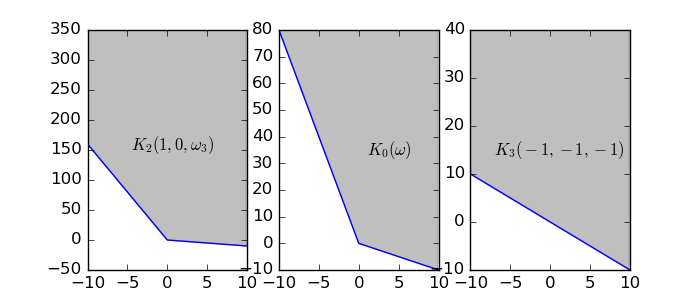
Figure 1: The solvency cones $K_{t}(\omega)$ for various $t$ and $\omega.$

We define our vector-valued objective function to be

$$U(x)=(-e^{-x_{1}},-e^{-x_{2}})^{T}$$

where $x=(x_{1},x_{2})^{T}$ is the quantity of physical assets we have at terminal time. Our set-valued objective function to be minimized is then

$$F(x)=\mathbb{E}\left[\left(e^{-x_{1}},e^{-x_{2}}\right)^{T}\right]+\mathbb{R}_{+}^{2}.$$

We assume that our initial endowment is $(0,0)^{T}$. The set of self-financing portfolios is

$$A_{3}=-K_{0}\mathbbm{1}-L^{p}(\sigma(\omega_{1});K_{1})-L^{p}(\sigma(\omega_{1},\omega_{2}),K_{2})-L^{p}(\sigma(\omega_{1},\omega_{2},\omega_{3}),K_{3})$$

where $K_{t}(\omega)$ are given as above.

We can then formulate the primal portfolio optimization problem as

$$\text{minimize }\mathbb{E}\left[\left(e^{-x_{1}},e^{-x_{2}}\right)^{T}\right]+\mathbb{R}_{+}^{2} \mathcal{P}_{ex}$$ ()

$$\text{subject to }x\in A_{3}$$

According to theorem (5.2), the dual problem is then

$$\sup\{z|\inf_{x\in L^{P}({\mathbb{R}}^{2},\mathcal{F}_{3})}z^{*}(\mathbb{E}\left[\left(-e^{x_{1}},-e^{x_{2}}\right)^{T}\right])+y^{*}(x)\leq z^{*}(z)\} \mathcal{D}_{ex}$$ ()

$$\text{subject to }y^{*}\in-A_{3}^{+}$$

$$z^{*}\in{\mathbb{R}}_{+}^{2}\setminus\{0\}$$

First, we investigate the nature of the set $-A_{3}^{+}$. From [12][Cor 16.4.2],

$$-A_{3}^{+}=(K_{0}\mathbbm{1}+L^{p}(\mathcal{F}_{1},K_{1})+L^{p}(\mathcal{F}_{2},K_{2})+L^{p}(\mathcal{F}_{3},K_{3}))^{+}$$

$$=\bigcap_{i=0}^{3}(L^{p}(\mathcal{F}_{i},K_{i}))^{+}.$$

In other words, $y^{*}\in L^{q}(\mathcal{F},{\mathbb{R}}^{2})$ is in $-A_{3}^{+}$ when $y(\omega)\in K_{t}(\omega)^{+}$ for each $t=0,...,3$.

We can explicitly compute the cones $K_{t}(\omega)^{+}$. We have that

$$K_{t}(\omega)=\text{cone}\left(\text{conv}\left\{\left(\begin{array}[]{c}1\\ -1\end{array}\right),\left(\begin{array}[]{c}-1\\ 8\cdot 2^{\sum_{i\leq t}\omega_{i}}\end{array}\right)\right\}\right)^{+}.$$

Hence the dual cone is

$$K_{t}(\omega)^{+}=\text{cone}\left(\text{conv}\left\{\left(\begin{array}[]{c}-1\\ -1\end{array}\right),\left(\begin{array}[]{c}-8\cdot 2^{\sum_{i\leq t}\omega_{i}}\\ -1\end{array}\right)\right\}\right).$$

Next we take the intersection of these cones to form $A_{3}^{+}(\omega)$. For a fixed $\omega$, let $s(\omega)=\min_{j=0,1,2,3}\sum_{i=1}^{j}\omega_{i}$. Then

$$-A_{3}(\omega)^{+}=\text{cone}\left(\left(\begin{array}[]{c}-1\\ -1\end{array}\right),\left(\begin{array}[]{c}-8\cdot 2^{s(\omega)}\\ -1\end{array}\right)\right).$$

Figure (2) illustrates $K^{+}_{t}(\omega)$ for various times and realizations of $\omega$.

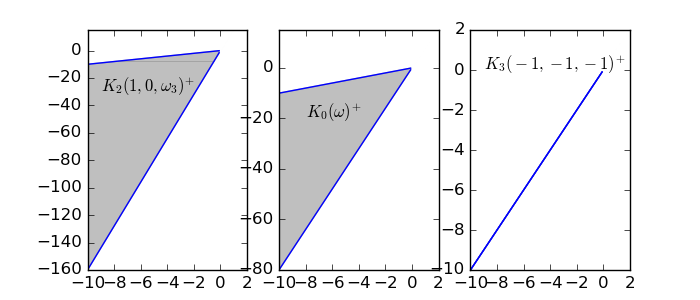
Figure 2: The positive polar cones $K_{t}(\omega)^{+}$ for various $t$ and $\omega.$

Now we work with to simplifiy the dual problem ($\mathcal{D}_{ex}$). The objective function is

$$h(y^{*},z^{*})=\left\{z|\inf_{x\in L^{p}(\mathcal{F},R^{2})}z^{*}(\mathbb{E}\left[(e^{-x_{1}},e^{-x_{2}})^{T}\right])+y^{*}(x)\leq z^{*}(z)\right\}$$

$$=\left\{z|\inf_{x\in L^{p}(\mathcal{F},R^{2})}\mathbb{E}\left[z_{1}^{*}\mathbbm{1}e^{-x_{1}}+z_{2}^{*}\mathbbm{1}e^{-x_{2}}\right]+y^{*}(x)\leq z^{*}(z)\right\}$$

Recall that the nature of linear functionals $y^{*}\in L^{q}(\mathcal{F},\mathbb{R}^{d})$ is $y^{*}(x)=\mathbb{E}\langle y^{*},x\rangle$. Hence the objective becomes

$$\left\{z|\inf_{x\in L^{p}(\mathcal{F},R^{2})}\mathbb{E}\left[z_{1}^{*}\mathbbm{1}e^{-x_{1}}+z_{2}^{*}\mathbbm{1}e^{-x_{2}}+y_{1}^{*}x_{1}+y_{2}^{*}x_{2}\right]\leq z^{*}(z)\right\}$$

Using the fact that our probability space is finite, we expand the expectation

$$\left\{z|\inf_{x\in L^{p}(\mathcal{F},{\mathbb{R}}^{2})}\frac{1}{27}\sum_{\omega\in\Omega}z_{1}^{*}e^{-x_{1}(\omega)}+z_{2}^{*}e^{-x_{2}(\omega)}+y_{1}^{*}(\omega)x_{1}(\omega)+y_{2}^{*}(\omega)x_{2}(\omega)\leq z^{*}(z)\right\}$$

This infimum is separable over the $x_{i}(\omega)$ variables. Hence,

$$=\left\{z|\frac{1}{27}\sum_{\omega\in\Omega}\inf_{x_{1}(\omega)\in{\mathbb{R}}}\{z_{1}^{*}e^{-x_{1}(\omega)}+y_{1}^{*}(\omega)x_{1}(\omega)\}+\inf_{x_{2}(\omega)\in{\mathbb{R}}}z_{2}^{*}e^{-x_{2}(\omega)}+y_{2}^{*}(\omega)x_{2}(\omega)\leq z^{*}(z)\right\}$$

We can compute each of these infimums explicitly. Note that

$$\inf_{x_{1}(\omega)\in{\mathbb{R}}}z_{1}^{*}e^{-x_{1}(\omega)}+y_{1}^{*}(\omega)x_{1}(\omega)=-f^{*}(-y_{1}^{*}(\omega))$$

where $f(x)=z_{1}^{*}e^{-x}$ and $f^{*}$ denotes the convex conjugate of $f$. Recall that for $g:\mathbb{R}\to\mathbb{R}$ and $a\in{\mathbb{R}}$ (See [12])

$$(ag(\cdot))^{*}(x^{*})=ag^{*}(x^{*}/a)$$

$$(g(a\cdot))^{*}(x^{*})=g^{*}(x^{*}/a)$$

$$g^{*}(x^{*}) =\left\{\begin{array}[]{ccc}x^{*}\ln(x^{*})-x^{*}&\text{ if }x^{*}>0\\ 0&\text{ if }x^{*}=0\\ \infty\text{ otherwise}\end{array}\right.\text{ when }g(x)=e^{x}.$$

Hence the objective function becomes

$$\left\{z|\frac{1}{27}\sum_{\omega\in\Omega}y_{1}^{*}(\omega)-y_{1}^{*}(\omega)\ln\left(\frac{y_{1}(\omega)^{*}}{z_{1}^{*}}\right)+y_{2}^{*}(\omega)-y_{2}^{*}(\omega)\ln\left(\frac{y_{2}^{*}(\omega)}{z_{2}^{*}}\right)\leq z^{*}(z)\right\}$$

when $y_{1}(\omega),y_{2}(\omega),z_{1},z_{2}\neq 0$.

Therefore, when $y_{1}(\omega),y_{2}(\omega),z_{1},z_{2}\neq 0$, we have the following formulation of the dual problem: find the supremum of

$$\left\{(z_{1},z_{2})^{T}\left|\frac{1}{27}\sum_{\omega\in\Omega}y_{1}^{*}(\omega)-y_{1}^{*}(\omega)\ln\left(\frac{y_{1}^{*}(\omega)}{z_{1}^{*}}\right)+y_{2}^{*}(\omega)-y_{2}^{*}(\omega)\ln\left(\frac{y_{2}^{*}(\omega)}{z_{2}^{*}}\right)\leq z_{1}^{*}z_{1}+z_{2}^{*}z_{2}\right\}\right.$$

subject to $$\left(\begin{array}[]{c}z^{*}_{1}\\ z^{*}_{2}\end{array}\right)\in{\mathbb{R}}^{2}\setminus\left\{\left(\begin{array}[]{c}0\\ 0\end{array}\right)\right\}$$

$$\left(\begin{array}[]{c}y^{*}_{1}(\omega)\\ y^{*}_{2}(\omega)\end{array}\right)\in A_{3}(\omega)\;\;\forall\omega\in\Omega$$

When either $z_{1}$ or $z_{2}$ equals $0$, we only consider $x_{2}$ or $x_{1}$, respectively, in our objective because the other terms vanish. Likewise, the case that $y_{1}(\omega)=0$ eliminates the expressions with $y_{1}(\omega)$ in the objective, because of the conjugation result on the previous page. The case that $y_{2}(\omega)=0$ is symmetric.

References

- [1] Mark HA Davis and Andrew R Norman “Portfolio selection with transaction costs” In Mathematics of Operations Research 15.4 INFORMS, 1990, pp. 676–713
- [2] F. Delbaen and W. Schachermayer “The Mathematics of Arbitrage”, Springer Finance Springer Berlin Heidelberg, 2006 URL: https://books.google.com/books?id=H3qCqENWeVgC
- [3] A. Hamel et al. “Set Optimization-a rather short introduction” In Set Optimization and Applications in Finance, Springer PROMS series, Forthcoming
- [4] Andreas H. Hamel “A Duality Theory for Set-Valued Functions I: Fenchel Conjugation Theory” In Set-Valued and Variational Analysis, 2009, pp. 153–182
- [5] Andreas H. Hamel and Andreas Löhne “Lagrange duality in set optimization” In J. Optim. Theory Appl. 161.2, 2014, pp. 368–397 DOI: 10.1007/s10957-013-0431-4
- [6] Andreas H Hamel, Andreas Löhne and Birgit Rudloff “Benson type algorithms for linear vector optimization and applications” In Journal of Global Optimization 59.4 Springer, 2014, pp. 811–836
- [7] Y.M. Kabanov “Hedging and liquidation under transaction costs in currency markets” In Finance and Stochastics 3.2 Springer-Verlag, 1999, pp. 237–248 DOI: 10.1007/s007800050061
- [8] Yu M Kabanov and Ch Stricker “The Harrison–Pliska arbitrage pricing theorem under transaction costs” In Journal of Mathematical Economics 35.2 Elsevier, 2001, pp. 185–196
- [9] Andreas Löhne, Birgit Rudloff and Firdevs Ulus “Primal and dual approximation algorithms for convex vector optimization problems” In Journal of Global Optimization 60.4 Springer, 2014, pp. 713–736
- [10] Michael JP Magill and George M Constantinides “Portfolio selection with transactions costs” In Journal of Economic Theory 13.2 Elsevier, 1976, pp. 245–263
- [11] Robert C Merton “Optimum consumption and portfolio rules in a continuous-time model” In Journal of economic theory 3.4 Elsevier, 1971, pp. 373–413
- [12] R.T. Rockafellar “Convex Analysis”, Princeton landmarks in mathematics and physics Princeton University Press, 1997
- [13] R.T. Rockafellar, M. Wets and R.J.B. Wets “Variational Analysis”, Grundlehren der mathematischen Wissenschaften Springer Berlin Heidelberg, 2010 URL: https://books.google.com/books?id=gvGLcgAACAAJ
- [14] Walter Schachermayer “The fundamental theorem of asset pricing under proportional transaction costs in finite discrete time” In Math. Finance 14.1, 2004, pp. 19–48 DOI: 10.1111/j.0960-1627.2004.00180.x
- [15] Steven E Shreve and H Mete Soner “Optimal investment and consumption with transaction costs” In The Annals of Applied Probability JSTOR, 1994, pp. 609–692
- [16] Sophie Wang with contributions from Andreas Hamel and Amit Singer “The Utility Maximization Problem in Markets with Transaction Costs: A Set-Valued Approach” Princeton University Senior Thesis, 2011