Jet Fragmentation via Recombination of Parton Showers

Abstract

We propose to model hadronization of parton showers in QCD jets through a hybrid approach involving quark recombination and string fragmentation. This is achieved by allowing gluons at the end of the perturbative shower evolution to undergo a non-perturbative splitting into quark and antiquark pairs, then applying a Monte-Carlo version of instantaneous quark recombination, and finally subjecting remnant quarks (those which have not found a recombination partner) to Lund string fragmentation. When applied to parton showers from the PYTHIA Monte Carlo event generator, the final hadron spectra from our calculation compare quite well to PYTHIA jets that have been hadronized with the default Lund string fragmentation. Our new approach opens up the possibility to generalize hadronization to jets embedded in a quark gluon plasma.

I Introduction

Hadron production from jets in high-energy collisions of hadrons or nuclei is often parameterized through fragmentation functions, using the universality of the process as given by factorization theorems of quantum chromodynamics (QCD) Collins:1981uw . On a microscopic level, hadron production in jets can be modeled very well through a perturbative evolution of the parton shower inside the jet using DGLAP splitting kernels to some low virtuality cutoff $Q_{0}$, followed by a non-perturbative hadronization model like the Lund string model or cluster hadronization applied to the parton shower. Event generators like PYTHIA Sjostrand:2006za and HERWIG Corcella:2002jc have successfully implemented such strategies to describe high momentum hadron production in $e^{+}+e^{-}$, $p+p$ and other processes.

In collisions of heavy nuclei at high energy, QCD factorization in jet hadronization is broken up to much higher hadron momentum, roughly 6-8 GeV/$c$ at typical collider energies, compared to the situation in elementary $e^{+}+e^{-}$ and $p+p$ collisions. This can be readily seen from the baryon enhancement measured in nuclear collisions both in Au$+$Au collisions at the Relativistic Heavy Ion Collider (RHIC) Adler:2003qi and in Pb$+$Pb collisions at the Large Hadron Collider (LHC) Abelev:2012wca . It has been suggested that hadron production at intermediate momenta, i.e. 2-8 GeV/$c$, can be described through the process of quark recombination or coalescence Greco:2003xt ; Fries:2003vb ; Greco:2003mm ; Fries:2003kq ; Fries:2004ej ; Fries:2008hs . It is an intriguing idea to combine the concepts of quark recombination and parton showers since recombination can be easily generalized to the hadronization of jets in dense environments as found in relativistic heavy ion collisions. In fact, quark recombination was applied to hadronization in jets in the early days of QCD Das:1977cp ; Chang:1980kh ; Migneron:1981cv , and more recently by Hwa and Yang Hwa:2003ic . However, parton showers in those early works were not obtained from the sophisticated parton Monte Carlo generators available today, but rather fitted to data or determined from specific models. In addition, earlier work also used event-averaged spectra, ignoring fluctuations coming from the small number of partons in each jet.

Here we show that essential aspects of hadron production in jet showers can be reproduced if we replace Lund string fragmentation in PYTHIA with an improved recombination model. We work with quarks and gluons at the end of their perturbative shower evolution, then let gluons decay into quark-antiquark pairs, evaluate quark recombination probabilities based on hadron Wigner functions by Monte Carlo sampling, and finally reapply Lund string fragmentation to those quarks which have not found a recombination partner. Finally, we compare our results to full PYTHIA results which simply hadronize entire showers by string fragmentation.

The paper is organized as follows. In the next section we describe how we prepare perturbative parton showers and extract the constituent quark distributions in phase space. In Sec. III, we describe the recombination model used in the present study and our treatment of remnant partons. In Sec. IV, we discuss our results and compare to full PYTHIA with string fragmentation. We conclude in Sec. V. Also included is an Appendix to derive the recurrence relation for the overlap integral between Gaussian wave packets and harmonic oscillator wave functions in the Wigner formalism used in the recombination calculation. Although in this work we deal strictly with jets in the vacuum, our motivation derives from the desire to generalize our approach to jets in a QCD medium later on Han:new .

II Parton Showers

    

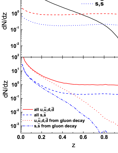
Figure 1: (Color online) Distribution $dN/dz$ of shower partons in terms of the momentum fraction $z$ of the initial jet momentum at the end of the perturbative shower evolution for a jet of 100 GeV before (upper panel) and after forcing gluon decays into quark-antiquark pairs (lower panel).

    

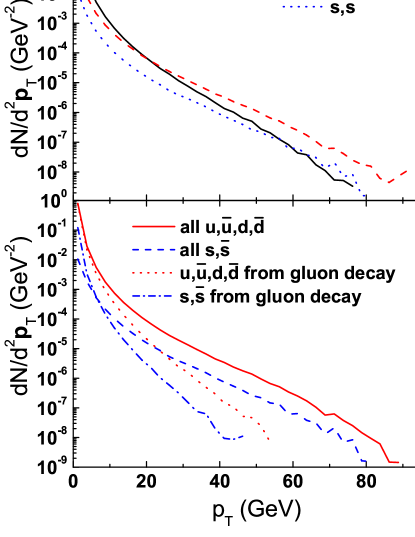
Figure 2: (Color online) Same as Fig. 1 for the shower parton transverse momentum distribution $dN/d^{2}{\bf p}_{T}$.

We are not concerned here with the mechanisms involved in creating parton showers. We use PYTHIA 6.3 Sjostrand:2006za as a tool to create perturbative parton showers as input to our hadronization procedure. PYTHIA 6.3 also serves as our benchmark for hadronization when we run pure Lund string fragmentation on the same ensemble of parton showers. Of course, another event generator that allows the extraction of shower partons from a jet before hadronization would work as well. Unless explicitly stated otherwise, the results presented here use monoenergetic jets of energy 100 GeV which are extracted from $e^{+}+e^{-}$ collisions at a center-of-mass energy of $\sqrt{s}=2E_{\mathrm{jet}}=200$ GeV in PYTHIA 6.3. By setting the cutoff for the perturbative evolution of the jet to $Q_{0}=1$ GeV, we extract the final parton configuration before string breaking. The upper panels of Figs. 1 and 2 show the resulting light quark ($u,d,\bar{u},\bar{d}$), strange quark ($s,\bar{s}$) and gluon ($g$) spectra as functions of their longitudinal momentum fraction $z$ in the jet and as functions of their momentum $p_{T}$ transverse to the jet axis, respectively. More precisely we define

$$z=\frac{\mathbf{p}\cdot\mathbf{P}_{\mathrm{jet}}}{|\mathbf{P}_{\mathrm{jet}}|^{2}},\quad p_{T}=\frac{\sqrt{|\mathbf{p}|^{2}|\mathbf{P}_{\rm jet}|^{2}-({\bf p}\cdot{\bf P}_{\rm jet})^{2}}}{|\mathbf{P}_{\rm jet}|}.$$ (1)

where $\mathbf{p}$ is the 3-momentum of the considered parton and $\mathbf{P}_{\mathrm{jet}}$ is the 3-momentum of the original parton creating the jet. The spectra $dN/dz$ and $dN/d^{2}{\bf p}_{T}$ are for one jet averaged over an ensemble of $10^{6}$ PYTHIA jets with $E_{\mathrm{jet}}=100$ GeV.

Since recombination models are usually built on the premise of dominance of the lowest Fock states in hadron wave functions, similar to hadronization in exclusive processes Lepage:1979zb ; Lepage:1980fj , only quarks and antiquarks are considered (see Ref. Muller:2005pv for a study on higher Fock states). Successful recombination models therefore postulate a (non-perturbative) splitting of gluons into quark-antiquark pairs. Using constituent quarks with masses $m_{u,d}=0.33~{}\rm{GeV}$ for light quarks and $m_{s}=0.5~{}\rm{GeV}$ for strange quarks, consistent with PYTHIA, we thus let gluons at the end of their perturbative evolution decay with their remaining virtualities between $2m_{u,d}$ and $m_{\mathrm{max}}$, where $m_{\mathrm{max}}>2m_{s}$ should be of the order of the scale $Q_{0}$. $m_{\mathrm{max}}$ is in principle a parameter and its value will mostly influence the ratio of strange to non-strange hadrons. We set this parameter to 1.25 GeV throughout this work. We decay gluons isotropically in their rest frame into $q\bar{q}$ pairs. The decay chemistry gives equal weight to $u\bar{u}$ and $d\bar{d}$ pairs for gluon virtualities between $2m_{u,d}$ and $2m_{s}$, while above the strangeness threshold the ratio of light to strange quarks is simply given by phase space and the vector nature of the decay as

$$\frac{\Gamma(g^{*}\to u\bar{u},d\bar{d})}{\Gamma(g^{*}\to s\bar{s})}=2\frac{m^{2}+2m^{2}_{u,d}}{m^{2}+2m^{2}_{s}}\sqrt{\frac{m^{2}-4m^{2}_{u,d}}{m^{2}-4m_{s}^{2}}}.$$ (2)

We do not consider heavy quarks in this study.

In PYTHIA, the final virtuality of shower gluons is forced to zero when the value becomes smaller than $Q_{0}$. While one could in principle undo this step, it turns out to be sufficient to reintroduce the non-perturbative gluon virtuality manually without rebalancing momenta in the last splitting. We find the typical error in total energy of the shower introduced this way is less than 1% for 100 GeV jets. The lower panels of Figs. 1 and 2 show the spectra of light and strange quarks from gluon decays for the same sample of 100 GeV jets used previously, together with the total light and strange quark spectra. The average number of quark and antiquarks in these 100 GeV jet showers after decays is about 13.

In principle, quark recombination could be formulated completely in momentum space (see Ref. Han:2012hp for applications to jet showers). However, for future applications in heavy ion collisions, where thermal partons will have nontrivial space-momentum correlations, we espouse a formulation of quark recombination employing Wigner functions with both momentum and space-time information. We are therefore led to introduce a space-time structure of showers. We do this based on two simple premises: (i) Virtual partons with virtuality $Q$ have an average life time $1/Q$ in their rest frame before splitting. This time is then properly boosted into the lab frame. (ii) The centers of wave-packets representing partons move on free classical trajectories given by the velocity $\mathbf{p}/E$ of the parton in the lab frame, where $E$ is the parton energy.

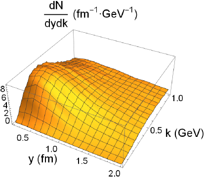
Figure 3: (Color online) Statistical distribution of quark-antiquark pairs in 100 GeV jet parton shower in terms of relative spatial and momentum coordinates $y$ and $k$ of the pair. The coordinates are defined in the common rest frame of the pair at the time the latter parton is created in the shower.

In the jet rest frame the spatial density of its shower partons depends on the time they are produced. However their density in momentum space is about 0.025/GeV³ and significantly smaller than the corresponding value of about 2.5/GeV³ for partons in a quark-gluon plasma at its phase transition temperature. One can analyze this parton initial state for hadronization more quantitatively. As we will discuss in detail in the next section, the decisive physical quantities for recombination between a particular quark and antiquark pair to occur are the relative distances $y$ and $k$ between the partons in space and momentum space measured at a common time in the rest frame of the pair. In Fig. 3 we show the statistical distribution of all quark-antiquark pairs we find in 100 GeV jet parton showers (normalized to one jet) as a function of their distances $y$ and $k$ in their common rest frame at the time when the latter parton of a pair is created. We find that this distribution peaks at $y\sim 0.5$ fm and $k\sim 0.3$ GeV, although large tails exist. This points to the existence of a “bulk” of partons in a jet shower which are quite close in phase space and amenable to recombination, while another, non-negligible fraction of partons will be far removed from other partons in phase space.

III Quark Recombination

Instantaneous quark recombination is most conveniently expressed in terms of an overlap of Wigner functions Fries:2008hs . The momentum distributions of mesons and baryons formed from recombination of quarks are generally given by

$$\frac{dN_{M}}{d^{3}{\mathbf{P}}_{M}} = g_{M}\int d^{3}{\bf x}_{1}d^{3}{\bf p}_{1}d^{3}{\bf x}_{2}d^{3}{\bf p}_{2}f_{q}({\bf x}_{1},{\bf p}_{1})f_{\bar{q}}({\bf x}_{2},{\bf p}_{2})$$ (3)

$$\times W_{M}({\bf y},{\bf k})\delta^{(3)}({\bf P}_{M}-{\bf p}_{1}-{\bf p}_{2})\,,$$

and

$$\frac{dN_{B}}{d^{3}{\bf P}_{B}} = g_{B}\int d^{3}{\bf x}_{1}d^{3}{\bf p}_{1}d^{3}{\bf x}_{2}d^{3}{\bf p}_{2}d^{3}{\bf x}_{3}d^{3}{\bf p}_{3}f_{q_{1}}({\bf x}_{1},{\bf p}_{1})$$ (4)

$$\times f_{q_{2}}({\bf x}_{2},{\bf p}_{2})f_{q_{3}}({\bf x}_{3},{\bf p}_{3})W_{B}({\bf y}_{1},{\bf k}_{1};{\bf y}_{2},{\bf k}_{2})$$

$$\times\delta^{(3)}({\bf P}_{B}-{\bf p}_{1}-{\bf p}_{2}-{\bf p}_{3})\,,$$

respectively. In the above, $f_{q}({\bf x}_{1},{\bf p}_{1})$ and $f_{\bar{q}}({\bf x}_{2},{\bf p}_{2})$ are the phase-space distribution functions of quarks and antiquarks, and they are normalized as $\int d^{3}{\bf x}d^{3}{\bf p}f_{q,\bar{q}}({\bf x},{\bf p})=N_{q,\bar{q}}$, where $N_{q,\bar{q}}$ is the quark or antiquary number. The Wigner functions of the meson and baryon (or antibaryon) are denoted by $W_{M}({\bf y},{\bf k})$ and $W_{B}({\bf y}_{1},{\bf k}_{1};{\bf y}_{2},{\bf k}_{2})$, expressed in terms of the relative coordinates and relative momenta of their valence quarks. For mesons, they are defined as

$${\bf y}={\bf x}_{1}-{\bf x}_{2},\quad{\bf k}=\frac{1}{m_{1}+m_{2}}(m_{2}{\bf p}_{1}-m_{1}{\bf p}_{2}),$$ (5)

where $m_{1}$ and $m_{2}$ are the masses of the quark and antiquark, respectively. For baryons (or antibaryons), while ${\bf y}_{1}$ and ${\bf k}_{1}$ are similarly defined as in Eq.(5), the second relative coordinate ${\bf y}_{2}$ and relative momentum ${\bf k}_{2}$ are given by

$${\bf y}_{2} = \frac{m_{1}{\bf x}_{1}+m_{2}{\bf x}_{2}}{m_{1}+m_{2}}-{\bf x}_{3},$$

$${\bf k}_{2} = \frac{m_{3}({\bf p}_{1}+{\bf p}_{2})-(m_{1}+m_{2}){\bf p}_{3}}{m_{1}+m_{2}+m_{3}},$$ (6)

with $m_{3}$ being the mass of the third quark (or antiquark). The meson and baryon Wigner functions are normalized as $(2\pi)^{-3}\int d^{3}{\bf y}d^{3}{\bf k}f_{M}({\bf y},{\bf k})=1$ and $(2\pi)^{-6}\int d^{3}{\bf y}_{1}d^{3}{\bf k}_{1}d^{3}{\bf y}_{2}d^{3}{\bf k}_{2}f_{B}({\bf y}_{1},{\bf k}_{1};{\bf y}_{2},{\bf k}_{2})=1$. The factor $g_{M}$ in Eq.(5) accounts for the probability for the color triplet, spin-$1/2$ quark and antiquark to form a given color singlet meson, while $g_{B}$ is the corresponding factor for three quarks (antiquarks) to form a given color singlet baryon (antibaryon). In the present study, the phase space functions of quarks and antiquarks will be replaced by the Wigner functions of individual quarks and antiquarks from the Monte Carlo jet shower generator, and we are going to use harmonic oscillator wave functions for hadrons to evaluate the momentum and space-time overlap integrals.

In Ref. Greco:2003xt for recombination of thermal partons among themselves and with jet partons, both the color and spin quantum numbers are treated on a purely statistical basis. The color flow in the parton shower is in principle tractable, although not yet implemented here for simplicity. Since the number of shower partons in a jet is very small, strong color correlations exist and the probability for colored shower partons to form color singlet hadrons is thus much larger than given by a statistical factor for colored thermal partons. For the present study we will neglect the statistical factors due to the color degrees of freedom and only include those due to the spin degrees of freedom. However, we prohibit the quark-antiquark pair from a forced gluon decay to recombine into a color-singlet meson. This approximation can be solidified by either invoking local color neutrality arguments Amati:1978by ; Corcella:2002jc , as also used for cluster hadronization in HERWIG, or a color octet approach, similar to the one used in heavy quarkonium production in nuclear reactions Wong:1999ur where color octet clusters are allowed to exchange soft gluons to convert into color singlets. Of course this could be improved in the future by following color flow in the parton shower simulation.

Because of their large relative momenta, shower partons are quite likely to recombine into excited hadron states. Wigner functions can have negative values, which makes them unsuitable for direct Monte Carlo evaluation. Instead we have to sample the quantum mechanical overlap integrals of the hadron Wigner functions with the Wigner functions representing the wave packets of shower partons, which we take to be Gaussians here. The resulting quantum mechanical overlap integral, which is guaranteed to provide a positive definite probability density that can be sampled, is equivalent to a Gaussian smearing of the Wigner functions in Eqs.(3) and (4), i.e., replacing $W_{M}$ by

$$\overline{W}_{M}({\bf y},{\bf k}) = \int d^{3}{\bf x}_{1}^{\prime}d^{3}{\bf k}_{1}^{\prime}d^{3}{\bf x}_{2}^{\prime}d^{3}{\bf k}_{2}^{\prime}$$ (7)

$$\times W_{q}({\bf x}_{1}^{\prime},{\bf k}_{1}^{\prime})W_{\bar{q}}({\bf x}_{2}^{\prime},{\bf k}_{2}^{\prime})W_{M}({\bf y}^{\prime},{\bf k}^{\prime}).$$

In the above, $W_{q}({\bf x}_{1}^{\prime},{\bf k}_{1}^{\prime})$ and $W_{\bar{q}}({\bf x}_{2}^{\prime},{\bf k}_{2}^{\prime})$ are, respectively, the Wigner functions of the quark and antiquark with their centroids at $({\bf x}_{1},{\bf k}_{1})$ and $({\bf x}_{2},{\bf k}_{2})$, respectively. The formula for baryons is analogous.

We can evaluate Eq.(7) with the help of some mathematics worked out in Appendix A. The result for a meson in the $n$-th excited state in the center of mass frame of the quark-antiquark pair is

$$\overline{W}_{M,n}(\mathbf{y},\mathbf{k})=\frac{v^{n}}{n!}e^{-v}.$$ (8)

with

$$v=\frac{1}{2}\left(\frac{{\bf y}^{2}}{\sigma_{M}^{2}}+{\bf k}^{2}\sigma_{M}^{2}\right).$$ (9)

where $\sigma_{M}$ is the width of the harmonic oscillator wave function for the relative motion of quark antiquark pair.

Similarly, the Gaussian smeared Wigner function for a baryon, with a wave function in the $n_{1}$-th excited state in one relative coordinate and in the $n_{2}$-th excited state in the other relative coordinate, is given by

$$\overline{W}_{B,n_{1},n_{2}}(\mathbf{y}_{1},\mathbf{k}_{1};\mathbf{y}_{2},\mathbf{k}_{2})=\frac{v_{1}^{n_{1}}}{n_{1}!}e^{-v_{1}}\cdot\frac{v_{2}^{n_{2}}}{n_{2}!}e^{-v_{2}},$$ (10)

with

$$v_{i}=\frac{1}{2}\left(\frac{{\bf y}_{i}^{2}}{\sigma_{Bi}^{2}}+{\bf k}_{i}^{2}\sigma_{B_{i}^{2}}\right),\quad i=1,2.$$ (11)

Since the wave functions of quarks and/or antiquarks in a hadron are always given in the rest frame of the hadron, we evaluate the relative coordinates and momenta in Eqs.(5) and (III) using the parton coordinates and momenta given at constant rest frame time Chen:2003ava ; Chen:2006vc in terms of their equal-time coordinates in the hadron rest frame. To this end, for each candidate partons to be treated their phase-space coordinates have to be Lorentz transformed from the lab frame to their common rest frame, and subsequently the partons produced earlier in the parton shower are propagated like free particles to the time at which the last candidate parton is produced and available for hadronization. We have checked that an algorithm that rather takes the distance of closest approach for the candidate partons has not much influence on the results as the parton shower is rapidly expanding.

The two width parameters $\sigma_{B1}$ and $\sigma_{B2}$ in the baryon Wigner function are related to each other by

$$\sigma_{B2}=\sigma_{B1}\left(\frac{\mu_{1}}{\mu_{2}}\right)^{1/2},$$ (12)

where the two reduced masses are defined as Oh:2009zj

$$\mu_{1}=\frac{m_{1}m_{2}}{m_{1}+m_{2}},~{}~{}\mu_{2}=\frac{(m_{1}+m_{2})m_{3}}{m_{1}+m_{2}+m_{3}}.$$ (13)

The width parameters of the harmonic oscillator wave function can be related to the measured size of the formed hadron. More precisely, for a meson consisting of quark and antiquark of masses $m_{1}$ and $m_{2}$ and quark charges $Q_{1}$ and $Q_{2}$, its mean-square charge radius is related to $\sigma_{M}$ by Oh:2009zj

$$\langle r^{2}\rangle_{M} = |\langle Q_{1}({\bf x}_{1}-{\bf X})^{2}+Q_{2}({\bf x}_{2}-{\bf X})^{2}\rangle|$$ (14)

$$= \frac{3}{2}\frac{|Q_{1}m_{2}^{2}+Q_{2}m_{1}^{2}|}{(m_{1}+m_{2})^{2}}\sigma_{M}^{2},$$

where ${\bf X}=(m_{1}{\bf x}_{1}+m_{2}{\bf x}_{2})/(m_{1}+m_{2})$ is the center of mass coordinate.

Similarly, the width parameter $\sigma_{B1}$ in the Wigner function of a baryon consisting of three quarks of masses $m_{1}$, $m_{2}$, and $m_{3}$, and charges $Q_{1}$, $Q_{2}$, and $Q_{3}$ are related to its mean-square charge radius is by Song:2012cd

$$\langle r^{2}\rangle_{B} = |\langle Q_{1}({\bf x}_{1}-{\bf X})^{2}+Q_{2}({\bf x}_{2}-{\bf X})^{2}+Q_{3}({\bf x}_{3}-{\bf X})^{2}\rangle|$$ (15)

$$= \frac{3\sigma_{B1}^{2}}{2(m_{1}+m_{2}+m_{3})}\left[\frac{m_{2}(m_{2}+m_{3})}{m_{1}+m_{2}}Q_{1}+\frac{m_{1}(m_{3}+m_{1})}{m_{1}+m_{2}}Q_{2}+\frac{m_{1}+m_{2}}{m_{3}}Q_{3}\right],$$

where ${\bf X}=(m_{1}{\bf x}_{1}+m_{2}{\bf x}_{2}+m_{3}{\bf x}_{3})/(m_{1}+m_{2}+m_{3})$ denotes the center of mass of the three quarks.

Table 1: Empirical charge radii $R_{c}$ (from Ref. Beringer:1900zz ), width parameters $\sigma_{M}$ or $\sigma_{B1}$, and spin statistical factors $g$ for hadrons used in the calculation.

Hadron	$R_{c}$ [fm]	$\sigma_{M}$ or $\sigma_{B1}$ [fm]	$g$
$\pi$	0.67	1.09	1/4
$\rho$	–	1.09	3/4
$K$	0.56	0.84	1/4
$K^{*}$	–	0.84	3/4
$N$	0.88	1.24	1/4
$N^{*}$	–	1.24	1/4
$\Delta$	–	1.24	1/2
$\Lambda$	–	1.21	1/4

We use measured charge radii for charged pions, protons and charged kaons to determine the width parameters $\sigma_{\pi}$, $\sigma_{K}$ and $\sigma_{N}$ in the pion, kaon and nucleon Wigner functions. The same width parameters are used for their isospin partners and their antiparticles as well as their spin resonances $\rho$, $K^{*}$, $N^{*}$, and $\Delta$. Since $\Lambda$ and $\bar{\Lambda}$ have no charge, their width parameters are determined instead from the matter radius, which is given by an equation similar to Eq. (15) after setting $Q_{1}=Q_{2}=Q_{3}=1/3$, and assuming that their size is the same as that of a proton. Excited states of these hadrons are then accounted for by the excited states of the harmonic oscillator wave functions using the same width parameters. In Table I we summarize the charge radii, width parameters and spin statistical factors for all stable hadrons and resonances included here.

Eqs. (A) and (10) can now be used to determine the recombination probability for a given quark-antiquark pair or a triplet of quarks or antiquarks. For a given shower, the relative coordinates in the common rest frame are evaluated for all possible hadron candidates which are subsequently accepted for recombination, or rejected, by Monte Carlo methods.

Some quarks might have quite small probabilities for recombination with any other parton in the same shower. In that case, there is a large probability that the Monte Carlo algorithm will not find a recombination partner. Such quarks are typically far removed from others in phase space, making all Wigner function overlap integrals small. The reason for this to occur is the lack of confinement in what is essentially a perturbative shower evolution. Of course isolated partons have to be connected by strings to another color charge and Lund string fragmentation can take care of their hadronization. We deal with such partons far removed in phase space by reconnecting them to other partons by QCD strings. This also includes undoing the non-perturbative gluon splitting introduced earlier, if none of the daughter quarks has found a recombination partner. We thus form short strings of the types $(q,\bar{q})$ and $(q,g,g,\ldots,\bar{q})$ and then hand them over to PYTHIA 6.3 for hadronization.

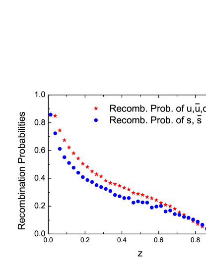
Figure 4: (Color online) Probabilities of light and strange quarks to recombine into hadrons as functions of their momentum fraction $z$ for100 GeV jets.

We end up with the following picture: Final hadron spectra are a mixture of hadrons from recombination (from quarks close in phase space to other quarks) and from string fragmentation (for quarks isolated in phase space or otherwise leftover). Typically, high-$z$ partons are both rare and far removed in phase space. They are unlikely to recombine with other partons in the shower (or partons from a surrounding medium if one would consider such). This can be seen in Fig. 4 where the probability of quarks to find a recombination partner is plotted as a function of parton momentum fraction $z$ for 100 GeV jets. Thus in our model moderate to high-$z$ partons still preferentially hadronize by string breaking. On the other hand, we indeed find the existence of a bulk of jet partons at lower $z$ in which quarks are close enough in phase space so that they prefer recombination. Recall that our main motivation is to establish a hadronization model which naturally generalizes to jets in a medium. It is now straightforward to see how our formalism can be applied to that more general case Han:new .

Excited states will be important channels for recombination. Excited mesons and baryons up to $n=5$ are known experimentally Beringer:1900zz . However, here we include the contributions from excited meson states up to $n=8$ and excited baryon states up to $n_{1}+n_{2}=8$, which can be easily done with harmonic oscillator wave functions. We allow excited states to decay to multiple pions in the case of light quark mesons, to kaon and pion in the case of light and strange mesons, to (anti)nucleon and pion in the case of light flavor (anti)baryons, and to $\Lambda$ and pion in the case of strangeness $\pm 1$ baryons. For decays into multiple pions, we determine their relative probabilities through the available phase space according to Milburn:1955zz

$$P_{l}(M)\sim\left[\frac{1}{6\pi^{2}}\left(\frac{M}{m_{\pi}}\right)^{3}\right]^{l}\frac{(4l-4)!(2l-1)}{(2l-1)!^{2}(3l-4)!}\,.$$ (16)

Here $l$ is the number of pions, $M$ is the mass of the excited state, or the invariant mass of the light quark-antiquark pair. The pion mass $m_{\pi}$ in the above equation comes from taking the radius of the emitting source to be that of the inverse of the pion mass Milburn:1955zz . In the present study, we replace $1/m_{\pi}$ by the distance between the recombined quark and antiquark, and consider its decay to at most four pions. The momentum distribution of these pions is then determined from phase space considerations. An excited nucleon $N^{*}$ or $\Delta$ decays to a nucleon and $l$ pions if its invariant mass is between $m_{N}+lm_{\pi}$ and $m_{N}+(l+1)m_{\pi}$ with $m_{N}$ being the nucleon masses. Again, we include at most four pions in the decay and use phase space considerations to determine their momenta. An excited kaon or $\Lambda$ is assumed to decay to a kaon or $\Lambda$ and multi-pions in a similar way.

IV Results

In the following, we compare results from our hadronization model applied to parton showers from PYTHIA 6.3 to calculations of PYTHIA with string fragmentation applied to the same parton showers.

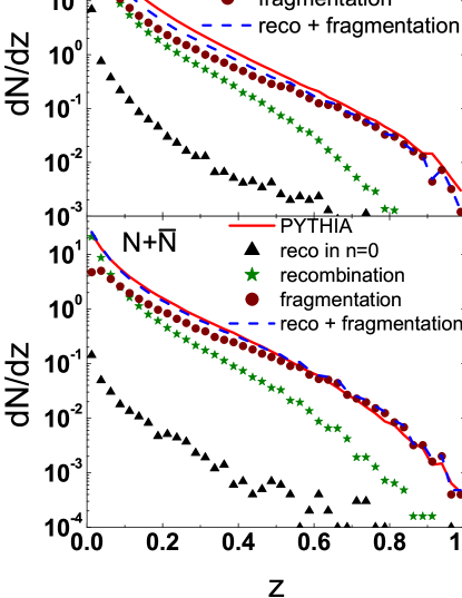
Figure 5: (Color online) Spectrum $dN/dz$ of pions (upper left panel), kaons (upper right panel), nucleons and antinucleons (lower left panel), and $\Lambda$ and $\bar{\Lambda}$ (lower right panel) from our calculation. Shown separately are contributions from the recombination of shower partons (stars) and fragmentation of remnant partons (circles). Also shown are the total contribution (dashed lines) and the results from PYTHIA string fragmentation (solid lines).

First, we test the longitudinal structure of jets by comparing the spectra $dN/dz$ as functions of the momentum fraction $z$ longitudinal to the jet axis for our sample of 100 GeV jets. In Fig. 5, we show the spectra of pions (upper left panel), kaons (upper right panel), nucleons and antinucleons (lower left panel), and $\Lambda$ and $\bar{\Lambda}$ (lower right panel) from 100 GeV quark jets. We show separately hadrons from recombined shower partons (stars), from the fragmentation of remnant hadrons (circles) and their sum (dashed line). The solid line indicates the result from PYTHIA 6.3 string fragmentation applied to the same sample of jet parton showers. We also show the recombination only through the ground state of the harmonic oscillator wave functions ($n=0$). As expected, we see that recombination spectra fall off faster with $z$ than the string fragmentation contribution. String fragmentation dominates at intermediate and high $z$ while recombination becomes the leading channel below $z\sim 0.1$, where the bulk of the hadron production resides.

We also note that recombination proceeds mainly through excited hadron states and not directly into $n=0$ ground state hadrons. The $n=0$ channel includes direct production of pion, kaon, nucleon, and $\Lambda$ as well as production from the the decay of $n=0$ spin-excited states $\rho$, $K^{*}$, $N^{*}$ and $\Delta$. The inclusion of excited states $n>0$ makes the recombination spectra considerably harder. Overall we find that the results from our model are consistent with spectra created by PYTHIA from pure string fragmentation. Note that the comparison to string fragmentation — another model — only makes sense on a qualitative level. Precision tuning of our model would have to involve fits to data which is outside the scope of this work. We compare the transverse momentum spectra of jets in Fig. 6. Again, results obtained from our hybrid recombination and fragmentation model compare well to pure string fragmentation.

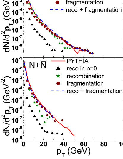
Figure 6: (Color online) Same as Fig. 5 for the transverse momentum spectra.

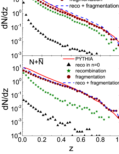
Figure 7: (Color online) Same as Fig. 5 for jets of energy $E_{\mathrm{jet}}=25$ GeV.

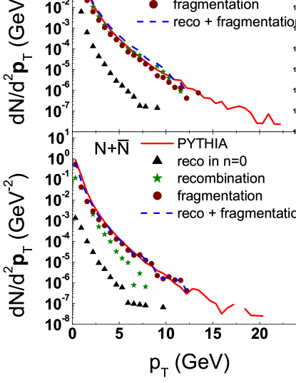
Figure 8: (Color online) Same as Fig. 6 for jets of energy $E_{\mathrm{jet}}=25$ GeV.

Finally we check our approach to hadronization with jets of a smaller jet energy and find again that our results reproduce pure string fragmentation reasonably well. The spectra for $E_{\mathrm{jet}}=25$ GeV jets are shown in Figs. 7 and 8 for the longitudinal and transverse momentum spectra, respectively. The recombination probability depends on the absolute distance of partons in phase space. Hence we expect the range in $z$ in which recombination competes with remnant string fragmentation to decrease with rising $E_{\mathrm{jet}}$. On the other hand, at smaller jet energies recombination stays more competitive out to larger $z$ at least for mesons, while for baryons the reduced number of partons in lower energy jets can lead to the opposite effect.

V Summary and Discussions

We have devised a model to hadronize perturbative parton showers in jets based on a hybrid of quark recombination and string fragmentation. Our algorithm reproduces results from pure string fragmentation and can be easily generalized to include partons from an ambient medium.

We turn perturbative parton showers into showers of constituent quarks and antiquarks by gluon decay. We then apply Monte Carlo methods to recombine quarks and antiquarks using probabilities given by their overlap integrals with respect to meson and baryon Wigner functions. The width parameters in these Wigner functions are fixed by hadron charge radii. Remnant quarks and antiquarks, which are not used for recombination, are connected by strings and subjected to the usual string fragmentation procedure in PYTHIA. We find that decays of excited states from recombination make the most important contributions to spectra of pions, kaons and nucleons.

We have checked that both the longitudinal and transverse momentum structures of hadron showers reproduce the results from PYTHIA string fragmentation. The only adjustable parameter that we have kept is the mass cutoff for gluon decays into quark-antiquark pair which can be set by the strange to non-strange hadron ratio. However, other quantities which are not very well known, like the width parameters in the Wigner functions for excited states of hadrons, can in principle be used as parameters for further fine tuning of results.

Our hybrid approach essentially keeps string dynamics intact for the high-$z$ tail of the jet and replaces string dynamics with recombination for the bulk of the jet where $\mathcal{O}(10)$ quarks with a few GeV/$c$ momentum can be found close enough together in phase space to recombine.

In the presence of a quark-gluon plasma produced in relativistic heavy ion collisions, we suggest that our approach can be generalized by sampling the ambient medium (e.g. provided by a fluid dynamic simulation into which the jet is embedded) for thermal partons. Recombination would be delayed if the ambient temperature is above the critical temperature $T_{c}$. At $T_{c}$ jet partons would be allowed to recombine with thermal partons, and remnant jet partons could also be allowed to connect to thermal partons by strings. This process, like other jet-medium interactions, would allow the exchange of energy and momentum. Details of an in-medium algorithm will be provided in a forthcoming manuscript Han:new .

Appendix A The Overlap of Gaussian Wave Packets with a Harmonic Oscillator

In this Appendix, we discuss details of the calculation of the overlap of harmonic oscillator Wigner functions and Gaussian wave packets. Let us start by noting that both Gaussian wave packets and the harmonic oscillator problem factorize into the three spatial directions. We can thus solve the corresponding one dimensional problem and then readily find the solution in three dimensions.

We start with the well known harmonic oscillator basis in one dimension MerzQM ,

$$\phi_{n}(x)=\left(\frac{m\omega}{\pi\hbar}\right)^{1/4}\frac{1}{\sqrt{2^{n}n!}}H_{n}(\xi)e^{-\xi^{2}/2},$$ (17)

where $\xi=\sqrt{\frac{m\omega}{\hbar}}x$, $H_{n}(\xi)$ are Hermite polynomials and $\omega$ is the oscillator frequency. The Wigner transformation of the harmonic oscillator wave functions, defined by

$$W_{n}(x,k)=\int^{\infty}_{-\infty}d\eta~{}e^{ik\eta}\phi_{n}\left(x+\frac{\eta}{2}\right)\phi_{n}\left(x+\frac{\eta}{2}\right),$$ (18)

leads to Groenewold:1946kp

$$W_{n}(u)=2(-1)^{n}L_{n}(u)e^{-u/2},$$ (19)

where $u=2\left(\frac{x^{2}}{\sigma^{2}}+\sigma^{2}k^{2}\right)$ with the width $\sigma=\left(\frac{\hbar}{m\omega}\right)^{1/2}$, and the $L_{n}$ are Laguerre polynomials.

We would like to calculate the overlap integral

$$\overline{W}_{n}(x,k) = \int dx_{1}^{\prime}dk_{1}^{\prime}dx_{2}^{\prime}dk_{2}^{\prime}$$ (20)

$$\times W(x_{1}^{\prime},k_{1}^{\prime})W(x_{2}^{\prime},k_{2}^{\prime})W_{n}(x,k),$$

of the Wigner function with Gaussian wave packets

$$W(x_{i}^{\prime},k_{i}^{\prime})=\frac{1}{\pi}e^{-(x_{i}^{\prime}-x_{i})^{2}/\delta^{2}}e^{-\delta^{2}(k_{i}^{\prime}-k_{i})^{2}},~{}i=1,2,$$

of width $\delta$ around centroids $x_{i}$ and $k_{i}$ in space and momentum. Here $x=x_{1}-x_{2}$ and $k=(k_{1}-k_{2})/{2}$, and the result will only depend on the relative position of centroids $r=x_{1}-x_{2}$ and $p=(k_{1}-k_{2})/{2}$.

Using the generating function for Laguerre polynomials MathMPhy ,

$$\frac{1}{1-t}e^{-\frac{tx}{1-t}}=\sum^{\infty}_{n=0}t^{n}L_{n}(x),$$ (22)

it is straightforward to see that Eq. (19) leads to the generating function for the oscillator Wigner functions

$$\frac{2}{1+t}\exp\left(-\frac{1-t}{2(1+t)}u\right)=\sum^{\infty}_{n=0}t^{n}W_{n}(u).$$ (23)

Carrying out the integrals from Eq. (20) on both sides of above equation, we obtain the following generating function for the Gaussian smeared Wigner function $\overline{W}_{n}$

$$\frac{2}{(1+t)(1+a\alpha)^{1/2}(1+a\alpha^{-1})^{1/2}}$$

$$\times\exp\left(-\frac{ax^{2}}{(1+a\alpha)\sigma^{2}}-\frac{ak^{2}\sigma^{2}}{1+a\alpha^{-1}}\right)=\sum^{\infty}_{n=0}t^{n}\overline{W}_{n}(x,k),$$

where $a=\frac{1-t}{1+t}$ and $\alpha=2\delta^{2}/\sigma^{2}$. By Taylor expanding the left hand side in $t$ and comparing coefficients of the same powers in $t$ on both sides, we obtain the following recurrence relation for the $\overline{W}_{n}$:

$$\overline{W}_{n+5} = -\frac{1}{\Lambda_{5}}(\Lambda_{4}\overline{W}_{n+4}+\Lambda_{3}\overline{W}_{n+3}+\Lambda_{2}\overline{W}_{n+2}$$ (25)

$$+\Lambda_{1}\overline{W}_{n+1}+\Lambda_{0}\overline{W}_{n}),$$

where $\Lambda_{i}~{}(i=0,1,\ldots,5)$ are given by

$$\Lambda_{0} = -[(1+\alpha)^{2}+n](1-\alpha)^{2},$$

$$\Lambda_{1} = [\alpha(1-\alpha)+2(x/\sigma)^{2}+2\alpha^{2}(k\sigma)^{2}+n+1](1-\alpha)^{2}x$$

$$\Lambda_{2} = [(1-\alpha)(\alpha^{2}+4\alpha+1)-2(x/\sigma)^{2}(3\alpha+1)$$

$$-2\alpha(k\sigma)^{2}(-\alpha^{2}+3\alpha+2)$$

$$-2(n+2)(1+\alpha)^{2}(1-\alpha)](1-\alpha),$$

$$\Lambda_{3} = [\alpha(1-\alpha)^{2}+2(x/\sigma)^{2}(3\alpha^{2}-2\alpha-1)$$

$$+2\alpha(k\sigma)^{2}(\alpha^{3}-3\alpha^{2}+9\alpha-7)$$

$$-2(n+3)(1+\alpha)^{2}(1-\alpha)^{2}],$$

$$\Lambda_{4} = [2(x/\sigma)^{2}+2\alpha^{2}(k\sigma)^{2}-(n+4)(1-\alpha)^{2}](1+\alpha)^{2},$$

$$\Lambda_{5} = -(n+5)(1+\alpha)^{2}.$$ (26)

Taking $\alpha=2\delta^{2}/\sigma^{2}=1$ for simplicity reduces Eq.(25) to

$$\overline{W}_{n+1}=\frac{v}{n+1}\overline{W}_{n},$$ (27)

with

$$\overline{W}_{0}=\exp(-v)~{}~{}{\rm and}~{}~{}v=\frac{1}{2}\left(\frac{x^{2}}{\sigma^{2}}+k^{2}\sigma^{2}\right)$$ (28)

or equivalently

$$\overline{W}_{n}=\frac{v^{n}}{n!}e^{-v}.$$ (29)

The Gaussian smeared $\overline{W}_{n}$ has the form of a Poisson distribution with the normalization

$$\sum^{\infty}_{n=0}\frac{v^{n}}{n!}e^{-v}=1,$$ (30)

which is similar to that of a coherent state sakurai .

In three dimensions, the Gaussian smeared Wigner function is thus given by

$$\overline{W}_{n}(\mathbf{x},\mathbf{k})$$

$$=\sum_{n_{x}+n_{y}+n_{z}=n}\overline{W}_{n_{x}}(x,k_{x})\overline{W}_{n_{y}}(y,k_{y})\overline{W}_{n_{z}}(z,k_{z})$$

$$=\sum_{n_{x}+n_{y}+n_{z}=n}\frac{v_{x}^{n_{x}}}{n_{x}!}e^{-v_{x}}\cdot\frac{v_{y}^{n_{x}}}{n_{y}!}e^{-v_{y}}\cdot\frac{v_{z}^{n_{z}}}{n_{z}!}e^{-v_{z}}$$

$$=\frac{1}{n!}e^{-v}\sum_{n_{x}+n_{y}+n_{z}=n}\frac{n!}{n_{x}!n_{y}!n_{z}!}v_{x}^{n_{x}}v_{y}^{n_{y}}v_{z}^{n_{z}}$$

$$=\frac{v^{n}}{n!}e^{-v},$$ (31)

with

$$v=v_{x}+v_{y}+v_{z}=\frac{1}{2}\left(\frac{{\bf x}^{2}}{\sigma^{2}}+{\bf k}^{2}\sigma^{2}\right).$$ (32)

The fourth equality in Eq.(A) follows from using the trinomial expansion formula

$$\sum_{n_{x}+n_{y}+n_{z}=n} \frac{n!}{n_{x}!n_{y}!n_{z}!}v_{x}^{n_{x}}v_{y}^{n_{y}}v_{z}^{n_{z}}$$ (33)

$$=(v_{x}+v_{y}+v_{z})^{n}=v^{n}.$$

References

- (1) J. C. Collins and D. E. Soper, Nucl. Phys. B 194, 445 (1982).
- (2) T. Sjostrand, S. Mrenna and P. Z. Skands, JHEP 0605, 026 (2006).
- (3) G. Corcella, I. G. Knowles, G. Marchesini, S. Moretti, K. Odagiri, P. Richardson, M. H. Seymour and B. R. Webber, hep-ph/0210213.
- (4) S. S. Adler et al. [PHENIX Collaboration], Phys. Rev. Lett. 91, 072301 (2003)
- (5) B. Abelev et al. [ALICE Collaboration], Phys. Rev. Lett. 109, 252301 (2012)
- (6) V. Greco, C. M. Ko and P. Levai, Phys. Rev. Lett. 90, 202302 (2003).
- (7) R. J. Fries, B. Muller, C. Nonaka and S. A. Bass, Phys. Rev. Lett. 90, 202303 (2003).
- (8) V. Greco, C. M. Ko and P. Levai, Phys. Rev. C 68, 034904 (2003).
- (9) R. J. Fries, B. Muller, C. Nonaka and S. A. Bass, Phys. Rev. C 68, 044902 (2003).
- (10) R. J. Fries, J. Phys. G 30, S853 (2004).
- (11) R. J. Fries, V. Greco and P. Sorensen, Ann. Rev. Nucl. Part. Sci. 58, 177 (2008).
- (12) K. P. Das and R. C. Hwa, Phys. Lett. B 68, 459 (1977) [Erratum-ibid. 73B, 504 (1978)].
- (13) V. Chang and R. C. Hwa, Phys. Rev. D 23, 728 (1981).
- (14) R. Migneron, L. M. Jones and K. E. Lassila, Phys. Rev. D 26, 2235 (1982).
- (15) R. C. Hwa and C. B. Yang, Phys. Rev. C 70, 024904 (2004).
- (16) K. C. Han, R. J. Fries and C. M. Ko, In Preparation.
- (17) G. P. Lepage and S. J. Brodsky, Phys. Lett. B 87, 359 (1979).
- (18) G. P. Lepage and S. J. Brodsky, Phys. Rev. D 22, 2157 (1980).
- (19) B. Muller, R. J. Fries and S. A. Bass, Phys. Lett. B 618, 77 (2005).
- (20) K. C. Han, R. J. Fries and C. M. Ko, J. Phys. Conf. Ser. 420, 012044 (2013).
- (21) D. Amati, R. Petronzio and G. Veneziano, Nucl. Phys. B 146, 29 (1978). doi:10.1016/0550-3213(78)90430-3
- (22) C. Y. Wong, Phys. Rev. D 60, 114025 (1999).
- (23) L. -W. Chen, C. M. Ko and B. -A. Li, Nucl. Phys. A 729, 809 (2003).
- (24) L. -W. Chen and C. M. Ko, Phys. Rev. C 73, 044903 (2006).
- (25) Y. Oh, C. M. Ko, S. H. Lee and S. Yasui, Phys. Rev. C 79, 044905 (2009).
- (26) C. M. Ko, T. Song, F. Li, V. Greco and S. Plumari, Nucl. Phys. A 928, 234 (2014).
- (27) J. Beringer et al. [Particle Data Group Collaboration], Phys. Rev. D 86, 010001 (2012).
- (28) R. H. Milburn, Rev. Mod. Phys. 27, 1 (1955).
- (29) E. Merzbacher, Quantum Mechanics, John Wiley & Sons, INC. (1998).
- (30) H. J. Groenewold, Physica 12, 405 (1946).
- (31) J. Mathews and R. L. Walker, Mathematical Methods of Physics, Addison-Wesley Publishing Company, Inc. (1970).
- (32) J. J. Sakurai, Modern Quantum Mechanics, Addison-Wesley Publishing Company, Inc. (1985).