Reaction diffusion patterns in Pseudoplatystoma fishes

Abstract

This paper studies how patterns derived from a system of reaction-diffusion equations may vary significantly depending on boundary and initial conditions, as well as in the spatial dependence of the coefficients involved. From an extensive numerical study of the BVAM model, we demonstrate that the geometric pattern of a reaction diffusion system is not uniquely determined by the value of the parameters in the equation. From this result, we suggest that the variability of patterns among individuals of the same specie may have its roots in this sensitivity. Furthermore, this study analyzes briefly how the inclusion of the advection and the space dependency in the parameters of the model influences the forms of a specific pattern. The results of this study are compared to the skin patterns that appear in Pseudoplatystoma fishes.

1 Introduction

Teolostei fishes exhibit a great diversity of pigmentation patterns. These patterns depend on the localization of pigmented cells, called chromatophores, which are originated in the neural crestpainter2001models . Those pigmented cells are mainly the xanthophores (of a yellow or orange color), melanophores (black), and iridophores (grey and silver) parichy2003pigment . The pigment cells migrate to the skin as an oscillatory perturbation until they reach their final location. Only when this migration is over, the cells acquire their characteristic pigment. Regions of skin dominated by a specific chromatophore turn into the respective color in such a way that the combination of those different regions forms a pattern Parichy2000 .

The mechanisms that establish the spatio-temporal organization of such patterns in fishes have not been determined conclusively. Kondo and Asai suggested that a reaction-diffusion (RD) mechanism of the Turing-type could explain this process Kondo1995 . The idea was that a RD mechanism provides a chemical pre-pattern between the chomotophores; this pattern is fixed to the skin through some morphogen, and, finally, cellular differentiation between regions of preponderance of one or other chromatophore gives place to the pattern on the skin of the fish. The results of that work, and of subsequent similar works that follow it, were figures that reproduce in good agreement the characteristics and the evolution of several fish patterns, see Refs. meinhardt2003algorithmic ; painter1999stripe ; varea1997confined .

More recently, Barrio and co-workers suggested a possible connection between a RD mechanism, called the BVAM model, and the patterns in the surubi fishes Barrio2009 . They showed that changing a single parameter in the model produce several kind of patterns, such as disordered dots, combinations of lines and dots, stripes and reticulated patterns, see Figure 1. In the same work, it was suggested the possibility of combining these basic forms in order to obtain the more elaborated patterns of the Pseudoplatystoma fishes.

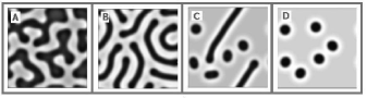
Figure 1: A change in the forms of the pattern of the BVAM model can occur by just changing the parameter $\delta$ in equation (1) : A) $\delta_{1}=$0.0, B) $\delta_{2}=$0.6 C) $\delta_{3}=$0.71 D) $\delta_{4}=$0.72. The other parameters are $\epsilon=0.65$, $\zeta=0.165$, $\gamma=-2.5$, $D_{0}=0.344$ and $\eta=0.15$. The domain is a square of size $L=80$ with zero flux boundary conditions. Taken from Ref. Barrio2009 .

Pseudoplatystoma is a group of neotropical catfishes of the family Pimelodidae which contains three long recognized species and another possible five species recently proposed buitrago2007taxonomy . These catfishes reach sizes that exceed 1.3 m, and live in various habitats such as large rivers, lakes and flooded neotropical forests buitrago2006anatomia . The systematic of this small group is unknown, in part because their species have large geographic variation in morphology and coloration. However, the pigmentation of three species is clearly different: the lateral region of the populations of P. fasciatum has dark vertical bands; P. tigrinum presents reticulated bands and P. coruscans features large dots arranged in rows in the lateral region of the body buitrago2007taxonomy , see Figure 2.

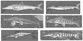
Figure 2: Species of Pseudoplayistoma Bleeker catfish. From top to bottom. Left: P. coruscans, P. fasciatum and P.tigrinum. Right: P. reticulatum, P. orinocoense and P. magdaleniatum. Taken from buitrago2007taxonomy .

Although the patterns obtained by Barrio and collaborators are quite similar to those present in the skin of the catfishes, there are some features that conventional reaction models, including the BVAM model, do not reproduce, for example: 1) the black and silver striped patterns on the fish have different thickness (except in the P coruscans); 2) some fish patterns have a preferred orientation, mainly to the vertical direction; and finally, 3) in some Pseudoplatystoma fishes occur a variation of the geometrical forms in the vertical direction, for example, the specks occurring only at the bottom of the P. oricoense or the reticulated on the top of P. reticulatum; see Figure 2.

We shall call conventional conditions to those that arise when using 1) fixed boundaries (not growing), 2) a closed domain, 3) constant coefficients in the reaction, and 4) random initial conditions around some fixed values (usually around the equilibrium points). Some few examples of those constraints in reaction diffusion models can be found in Refs. dufiet1992numerical ; madzvamuse2006time ; pearson1993complex ; ruuth1995implicit .

In this work, we go beyond previous reaction-diffusion models, formulated with the aim to reproduce skin patterns observed in animals (such as the Pseudoplatystoma catfishes), by analyzing the effect of some external factors that may influence their time evolution and final shapes. Here, by external factors we mean those which are not included in the reaction-diffusion equations. More specifically, we will show that the morphology of the patterns depends crucially on: 1) different boundary and initial conditions; 2) the effect of advection, and 3) space dependent kinetic parameters. These factors are frequently found in real biological conditions and are very important in the spatio-temporal progress of pattern formation. Thus, even though the BVAM model Barrio2009 reproduces the irregular arrangement of stripes and points observed on the catfishes, we will show that changing the values of the parameters of the reaction mechanism is not sufficient to explain the spatial dependence of the shapes and their orientation. On the contrary, we will show that is suffices to consider combinations of the three factors mentioned above to reproduce more readily and accurately the skin patterns observed in the Pseudoplatystoma catfishes.

The organization of this work is the following. In Section 2, we present the BVAM model and the basic patterns derived from it using standard boundary and initial conditions. In Section 3, we introduce different boundary and initial conditions for a reaction scheme with the same configuration at the parameter space, and see how the original patterns are modified. Furthermore, we will explore the effect of advection on the patterns and the spatial dependency of the kinetic parameters of the reaction in the BVAM model. In Section 4 we will compare the patterns obtained in the previous section with those of the Pseudoplatystoma fishes. Finally, in Section 5, we will present the final conclusions of this work.

2 The BVAM reaction diffusion model and its numerical approximation

The interactions among morphogenes within living organisms can be conceptualized as two coupled processes involving chemical reactions and differential diffusion. Thus, reaction diffusion models seem to be appropriate quantitative schemes for reproducing the spatial distribution of these morphogenes previous to their manifestation as a given pattern on, for instance, the skin of organisms. In this context, a very useful model that allows one to obtain a wide variety of patterns is the BVAM model, proposed originally in barrio1999two . In this model, the authors suggested that, near the equilibrium concentration of both morphogenes (located at the origin), the interaction between both components could be sufficiently described as a third order reaction. This reaction scheme, together with an unequal diffusion of both morphogenes, $u$ and $v$, gives place to a reaction-diffusion model which, in its dimensionless form, can be written as Barrio2009 :

$$\frac{\partial u}{\partial t}=D\nabla^{2}u+\eta(u+\alpha v-\delta uv-uv^{2}),$$ (1a)

$$\frac{\partial v}{\partial t}=\nabla^{2}v+\eta(\beta v+\gamma u+\delta uv+uv^{2}).$$ (1b)

The spatial scale was normalized with the characteristic length of the domain whereas time was normalized with a combination of the diffusion coefficient of the morphogen $v$ and the spatial scale Barrio2009 . Thus, $D=D_{u}/D_{v}$ is the ratio of the diffusion coefficients associated to both morphogenes,and $\eta$ provides the characteristic spatio-temporal scale of the pattern formation process. The coefficients $\alpha$, $\beta$, $\delta$ and $\gamma$ are adjustable parameters which determine the appearance and form of the patterns.

The idea of using a third order reaction scheme is that it provides three different fixed points, providing of great richness to the variety of patterns obtainable by the model Barrio2009 . Besides the origin $(u_{0},v_{0})=(0,0)$, the additional two fixed points are $(u_{0},v_{0})=(-\zeta,1)w_{\pm}$, where $w_{\pm}$ is given by:

$$w_{\pm}=\frac{-\delta\pm\sqrt{\delta^{2}+4\epsilon}}{2},$$ (2)

and $\epsilon$ and $\zeta$ are defined as $\epsilon=\beta/\zeta-\gamma$ and $\zeta=(\alpha+\beta)/(1+\gamma)$.

A detailed study of this model can be found in Ref. varea2007soliton . The main conclusion is that the model produces different patterns, ranging from spots to strips, by just changing one single parameter, namely $\delta$, see Figure 1. Furthermore, numerical simulations confirm that a great variety of stationary and transient patterns can be obtained from the BVAM scheme Barrio2009 ; barrio1999two . Of particular interest to our work are the striped-like patterns, and those that contain some disorderly dots, as shown in Figure 1, since they are present in Pseudoplatystoma fishes.

In this study we have developed our own numerical solvers, employing different approximation schemes, mainly based on the finite difference method and on the finite element method thesis . We have been able to reproduce several patterns previously reported in the literature for the BVAM model and others, validating in this way our codes. Due to its better approximation properties and its flexibility to deal with boundary conditions, in the present study we employed a finite element method for space discretization, and a semi-implicit Euler scheme to integrate the discrete models in time. This numerical scheme is implicit for the diffusion term and explicit for the reaction terms. The details can be found in thesis .

In Figure 3, we show a set of patterns extending those shown in Figure 1, by considering a wider range of the parameters $D$, $\eta$, and $\delta$ in equations (1). We have confirmed the appearance of dots, stripes and reticulated patterns for the BVAM model for conventional conditions, i.e., zero flux boundary conditions, random initial conditions near the equilibrium point (0,0), and constant kinetic parameters along the entire domain.

However, it is convenient to emphasize that those computed patterns do not exhibit the preferential orientation present in some of the Pseudoplatystoma fishes. In the next section, we will focus our attention in the mechanisms inducing changes in a pattern obtained with some specific set of parameters. In particular, we will analyze the problem of how these changes could contribute to the orientation of the basic geometrical forms of a pattern.

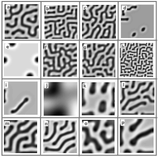
Figure 3: Patterns (not necessarily stationary) of the BVAM model in a square domain of size $L=80$, after a time of T=750. Initial conditions are given by both concentrations near the equilibrium value $(0,0)$, with a random addition of maximum amplitude $0.05$. Furthermore, we use zero flux boundary conditions at the four boundaries. The value of the parameters $\epsilon,\zeta$ and $\gamma$ are the same as the previous figure. The triad of parameters $(D,\delta,\eta)$ are given as: a(0.344; 0.72; 0.225), b(0.172; 2.0; 0.1), c(0.172; 0.8; 0.15), d(0.344; 1.5; 0.3), e(0.516; 0.72; 0.15), f(0.172; 0.00; 0.15), g(0.172; 0.72; 0.15), h(0.172; 3.5; 0.15), i(0.344; 1.55; 0.15), j(0.344; 1.7; 0.15), k(0.344; 0.72; 0.075), l(0.344; 0.0; 0.225), m(0.344; 0.0; 0.15), n(0.344; 1.4; 0.15), o(0.516; 0.0; 0.15), p(0.516;0.36; 0.15). Numerical simulations were made using Finite Element method with a mesh of 3200 triangles and a step size of $\Delta t=5\times 10^{-2}$. The detail of the numerical method used in reaction-diffusion systems could be found in thesis .

3 Patterns under non-conventional conditions

3.1 Initial conditions

It is noteworthy that, despite the great attention that reaction diffusion systems have had in recent years in the study of pattern formation, little has been studied about the influence of initial and boundary conditions in the solution of the problem, although they are factors that complement the mathematical model and may play an important role in the type of solutions obtained arcuri1986pattern . Our interest in this section is to examine how these two factors could produce a vertical orientation on the stripes, and to show how the variation of initial conditions could produce very different patterns, in spite of using the same parameter set.

The initial conditions more often used in these types of problems are obtained by adding a random contribution to both concentrations placed at their equilibrium values (see for example barrio1999two ; dufiet1992numerical ). In that case, the orientation of the striped-like patterns can occur in at least two ways: 1) using boundary conditions of the Neumann type that aligns the stripes parallel or perpendicular to the boundaries, or 2) adding some preferential direction to the initial conditions dufiet1992numerical ; madzvamuse2006time ; ruuth1995implicit .

The influence of the initial conditions on the solutions obtained with the BVAM model of equations (1) is shown in Figure 4. In this figure, the temporal evolution of the pattern is tracked from the initial condition (at the left of each row), until the stationary pattern (at the right), with three intermediate states. We emphasize that all other data in the model were maintained fixed, like the size of the domain, the boundary conditions (Neumann, zero flux) and the set of parameters. The specific information about the initial conditions used in each case is the following:

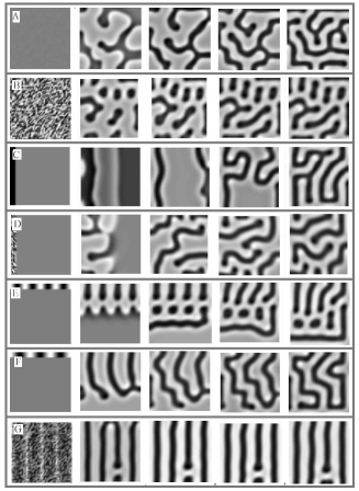
Figure 4: Different patterns obtained varying only the initial conditions. The left column shows the initial condition; the intermediate columns show three intermediate states, and on the right the stationary pattern obtained after a time $T$, given in each case by: A) 875 B) 875 C) 5000 D) 875 E) 5000 , F) 4000, G) 500. The domain is also a square of side 80 and the reaction parameters were the same as Figure 1.B for all cases.

1. .- We first compare the rows 4.A and 4.B where we have used conventional random initial conditions, with the only difference that the noise intensity is different in each case. In Figure 4.A, the initial values $u$ and $v$ are between $\pm 0.001$, whereas in 4.B are between $\pm 0.1$. The results show that the obtained stripes are (on average) longer in the former case than in the latter, where some spots look more like dots than as stripes.

2. .- Now, we compare the rows 4.C and 4.D. In both cases, the concentrations of the two morphogenes are zero except in a small strip on the left side of the square. In the first case, the initial condition is a left vertical stripe with $u=-0.1$ and $v$ randomly distributed, while in the second case, both concentrations are random with a maximum amplitude of $0.05$. In both cases, the disturbance spreads to the other side of the domain. However, the wave front in 4.C proceeds as a vertical strip, which is duplicated and bounces off at the right vertical boundary to form a labyrinth type form. In the second case, 4.D, the disturbance advances in disorder, even with a slight preference for the horizontal direction, giving, at the end, a similar pattern to 4.B, but more disorganized.

3. .- Next, we compare Figures 4.E and 4.F. In this case, the initial concentration of both morphogenes is zero almost everywhere, except for a stripe at the top of the domain. In the first case, this strip consists of four cosine oscillations of $u$ while the other has only three. The amplitude of the oscillations is $0.05$. The variable $v$ is randomly distributed in this strip and zero outside. In the case of 4.E, stripes and spots move downward preserving the same arrangement of columns, whereas in the case 4.F the strips disperse and form a pattern similar to that in 4.C. Other choices of the number of initial oscillations leads to results similar to those of 4.F.

4. .- Finally, we present an initial pattern with four stripes completely ordered, as shown in Figure 4.G. These initial conditions consist of four vertical oscillations, plus random noise for both variables. These oscillations are taken with a maximum amplitude of 0.05. The almost perfect vertical orientation vanishes when the number of initial oscillations is different to four. In this case, the stripes fade, forming a pattern rather similar to that in Figure 4.D, without any preferential orientation.

The previous results allow us to conclude that: 1) Neumann boundary conditions tend to align the patterns with the edges; 2) the forms of the pattern may travel as a perturbation and stay or fade depending upon the initial condition; and finally, 3) the results obtained in 4.E and 4.G suggest that only specific initial conditions (an ordered chemical pre-pattern) of the morphogenes can yield specific orientations of the stripes, like those observed in live organisms. This suggests, in turn, that a previous chemical reaction diffusion mechanism may be necessary to establish an ordered chemical pattern. In this form, the development of a complex organ, like the skin, occurs as a series of stages that involve different time scales and activation/deactivation subprocesses.

3.2 Boundary conditions

Another aspect to consider is the type of boundary conditions used. Conventionally, either zero flow or periodic boundary conditions have been imposed on all the boundaries of the domain to demonstrate the existence of patterns dufiet1992numerical ; madzvamuse2006time . In our case, considering the form of Pseudoplatystoma fish, we may assume that a combination of both types of boundary conditions could model better the spatial disposition of the resulting patterns along the body of the fish. Because the pattern in the fishes are spatially repeated from the end of the head (operculum) to the root of the tail (caudal fin), see Figure 2, we propose a domain with no flow through the horizontal boundaries (top and bottom), and periodic conditions on the vertical edges.

However, as we show in Figure 5, the election of the boundary conditions not necessarily affects the type of pattern obtained. For the results shown in this figure, we have employed four combinations of boundary conditions without any significant alteration of the geometrical form (stripes) obtained in Figure 1.B. The same statement is also true for the other three kind of patterns of the Figure 1. Therefore, we conclude that the election of boundary conditions does not significantly affect the formation and appearance of the pattern, at least for the cases we have studied here.

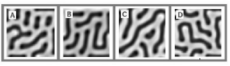
Figure 5: Patterns obtained by varying only the boundary conditions. In each case, these are given by: A) Neumann, zero flux, B) Neumann, with a current source 0.05 in the upper border, C) periodic, and D) Left and right edges are periodic, and zero flux up and down. Patterns are taken after a time T = 350. The parameters are the same as in Figure 1.B.

3.3 Space dependent coefficients

In this section, we will explore the spatial variation of the parameters of the chemical reaction of the BVAM model. The aim is to create combinations of the basic patterns of the BVAM model, which are sown in Figure 1, in order to obtain the complex patterns appearing in the Pseudoplatystoma fishes shown in Fig. 2.

To achieve this objective, we have varied the coefficients $\eta$ and $\delta$ spatially. We select these parameters because it is well known how the shape of the patterns changes with their variation. We want to make clear that we will not consider a spatial variation of the diffusion coefficient $D$. Nevertheless, in previous works it has been proven that an anisotropic diffusion can generate orientated patterns sanderson2006advanced ; shoji2002directionality . Those models assume that each of the substances have a preferential direction to spread.

To construct a spatial variation of $\delta$, we consider the four different patterns that arise with the BVAM model when different constant values of this parameter are imposed Barrio2009 . Those patterns are 1) reticulated, 2) stripes, 3) dots and stripes, and 4) disordered dots, and they are obtained at specific values that we have labeled as $\delta_{1}$, $\delta_{2}$, $\delta_{3}$, $\delta_{4}$, respectively, as shown in Figure 1. The idea in this section is that the transition between a specific kind of pattern and other in the same figure could be obtained by changing the value of the parameter $\delta$ spatially.

On the other hand, to construct a spacial variation of $\eta$, we have to take into account that, in the dimensionless form of a reaction diffusion system, like that of equations (1), the value $\eta$ provides a spatio temporal scale proportional to $L^{2}/t$, in such a way that, if the size of the domain $L$ is fixed, increasing $\eta$ represents a decrease in the size of the pattern shape and an increase in the reaction rate Murray2003 .

The results of our numerical experiments, when spatial variation is incorporated to $\eta$ and $\delta$, are summarized in Figure 6, which we proceed to explain row by row:

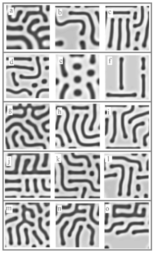
Figure 6: Patterns with spatial dependence in the parameters $\eta$ and $\delta$. The other parameters are the same as Figure 1. See text for details.

1. .- The first row of Figure 6 presents the results obtained when $\eta$ increases linearly according to

   $$\eta(y)=0.15+(0.40-0.15)\frac{y}{L}.$$ (3)

   The other parameters are the same as those used to obtain the results shown in Figures 1.A, 1.B and 1.D, respectively, where $\eta$ had the fixed value of 0.35. It is clear that an increase of $\eta$ causes a change in the size of the spots (Figure 6.a) and stripes (Figure 6.b) without a significant change in form. However, in the case of dots, the gradient of $\eta$ causes that they become stripes (Figure 6.c).

2. .- In the second row of Figure 6, we show results obtained when parameter $\delta$ oscillates around two typical values for which stripes and dots are obtained with the BVAM model, (i.e., around $\delta_{3}=0.71$ and $\delta_{5}=0.80$, respectively). These oscillations are imposed in the horizontal direction in the form:

   $$\delta(x)=\delta_{3}+(\delta_{5}-\delta_{3})\sin^{2}{\left(\frac{\pi mx}{L}\right)},$$ (4)

   where $m=2,3,4$ determines the number of oscillations of $\delta$ for Figures 6.d, 6.e, and 6.f, respectively. It is noted that the vertical orientation is retained only for the cases 6.e and 6.f, while in Figure 6.d, the spots and stripes are intermingled haphazardly.

3. .- In the third row of Figure 6, we present results that show the effect of decreasing $\delta$ linearly between two different typical values where a pattern change occurs, see Figure 1. A spatial variation of $\delta$ in the vertical direction is given by

   $$\delta(y)=\delta_{n+1}+(\delta_{n}-\delta_{n+1})\frac{y}{L},$$ (5)

   with $n=1,2,3$ for Figures 6.g, 6.h, and 6.i respectively. We expected to obtain the following transitions: from spots to stripes, from stripes to stripes and dots, and finally, the transition from stripes to just dots, respectively. However, this did not occur due to the fact that the gradient of $\delta(y)$ tends to elongate all the forms into stripes.

4. .- The fourth row is the same as above, except that now the variation of $\delta$ in the vertical direction is given by a jump at $y=L/2$. More specifically:

   $$\delta(y)=\begin{cases}\delta_{n}&\mbox{if }y\geq L/2,\\ \delta_{n+1}&\mbox{if }y<L/2.\end{cases}$$ (6)

   with $n=1,2,3$ for Figures 6.j, 6.k, and 6.l respectively. This particular form of the parameter $\delta$ causes the overlapping of shapes and the distortion of the dots, except in Figure 6.j where there are two distinct regions. This is because the difference between $\delta_{1}$ and $\delta_{2}$ is much grater (in absolute value) than in the other cases.

5. .- Finally, in the last row of Figure 6, we present combinations of the previous cases.

   In Figure 6.m, we present the result obtained with a linear change of $\delta$, which includes the values covering the entire range from spots to dots:

   $$\delta(y)=\delta_{4}+(\delta_{1}-\delta_{4})\frac{y}{L}.$$ (7)

   In Figure 6.n we present the result obtained with a variation of $\delta$, combining oscillations in the horizontal direction (like those of Fig. 6.e), and a linear decrease in the vertical direction (like that of Fig. 6.g). For this last case, the spatial variation of $\delta$ is given by

   $$\delta(x,y)=\left[(\delta_{4}-\delta_{1})-(\delta_{4}-\delta_{2})\cos^{2}{\left(\frac{3\pi x}{L}\right)}\right]\frac{y}{L}.$$ (8)

   Figure 6.o is similar to Figure 6.m but now the spatial variation of $\delta$ in the vertical direction is a piecewise constant function defined by:

   $$\delta(y)=\begin{cases}\delta_{1}&\mbox{if }y\geq 2L/3,\\ \delta_{2}&\mbox{if }2L/3>y>L/3.\\ \delta_{4}&\mbox{if }y\leq L/3.\end{cases}.$$ (9)

   In these last three cases, we obtained the combination of different forms in the same pattern, and is noteworthy that the change is more marked when the coefficients are discontinuous.

From the results of this part of the section, we can conclude that the spatial variation of the kinetic parameters allows us to obtain a somewhat larger combination of patterns. However, the occurrence of stripes with dots in the same pattern is very difficult to obtain by following this strategy. One of the reasons is that the gradient of one parameter ($\delta$ or $\eta$ in our case) tends to elongate the dots and turn them into stripes. Therefore, in the next section, we will consider another possibility for obtaining the combination of stripes and dots, and a preferential orientation in a pattern.

3.4 Effect of advection

In general, the information that exists about the mechanisms that lead to the formation of the patterns of the Pseudoplatystoma and their diversity is very scarce. For example, it is known that the pigmentation begins to show at nine days of age. This pigmentation appears, first, in the head part, until it is clearly defined in the body at the tenth day, see Figure 7. It is also believed that the initial peculiar pattern of post-larvae is kept for two and a half months until it takes its final form. This pattern serves to camouflage the fish as a defense when they are dragged into the flooded river banks, where the vegetation provides ideal sites for concealment perez2001reproduccion .

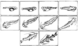
Figure 7: Stages of larval development. It is up to the ninth day that the pigmentation start to be noticed, mainly in the head. Taken from Ref. perez2001reproduccion

The fact that the coloration appears first in the head, and then is dispersed along the entire skin, suggests the possibility of an underlying transport process besides the reaction diffusion interaction. In this section, we explore the possibility that the interaction between both morphogenes may be influenced by an advective sub-process along the fish skin. Specifically, we will show that the advection could be seen as a possible origin of the preferential orientation of some fish patterns.

In view of these considerations, we add an advective term to the original reaction diffusion system described in equations (1), obtaining as a result a reaction convection system for the BVAM model of the form galeano2013formacion :

$$\frac{\partial u}{\partial t}+\mathbf{z}\cdot\nabla u=D\nabla^{2}u+\eta(u+\alpha v-\delta uv-uv^{2}),$$ (10a)

$$\frac{\partial v}{\partial t}+\mathbf{z}\cdot\nabla v=\nabla^{2}v+\eta(\beta v+\gamma u+\delta uv+uv^{2}).$$ (10b)

We are particularly interested in a vertical advective flux through the term $\mathbf{z}=z\hat{e_{y}}$, with $z$ a constant parameter for the volumetric velocity of both morphogenes, and $\hat{e}_{y}$ the unitary vector in the vertical direction.

In Figure 8, we show the results obtained by adding the effect of advection to the original patterns of Figure 1. As it is shown, advection in the vertical direction introduces not only the desired orientation on the patterns, but also the combinations of dots and stripes, as we have previously searched for some of the Pseudoplatystoma fishes.

We can see that, for all cases, the orientation of the pattern tends to align along the direction in which advection takes place. Also, in the same figure, it can be observed that dots are present in the final pattern, at the end of the lines, as long as somehow they are present in the parameter set chosen.

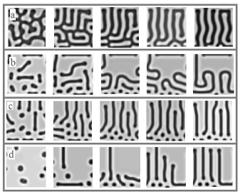
Figure 8: Results obtained with the same four set of parameters of Figure 1, but with the effect of advection in the vertical direction. For these simulations, we used $\mathbf{z}=0.02\hat{e}_{y}$ in equations (10). At the beginning (left column), the pattern resembles the reaction diffusion pattern of Fig. 1, but as time goes, the advection aligns the forms (right column). The simulations use zero flux boundaries conditions at the top and bottom boundaries, and periodic boundary conditions at both vertical sides.

4 Comparison with patterns in Pseudoplatystoma fishes

In this section we compare the lateral region of the Pseudoplatystoma fishes with some of the most similar patterns obtained previously with numerical solutions of the BVAM model, see Figure 9:

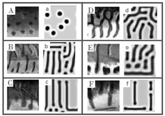
Figure 9: Comparison between the pattern in the skin of the Pseudoplatystoma fishes (capital letters) and some of the patterns derived from numerical simulation of the BVAM model (lower case letter). See text for details.

1. .- In the case of P. coruscans (Figure 9.A), the pattern presents semicircular spots horizontally staggered, with some elongated spots on the top. This suggests that these patterns can be obtained with the conditions of Figure 1.D, but with some kind of horizontal dependency in the parameters to give regularity in the horizontal direction.

2. .- In the case of P. reticulatum (Figure 9.B), the pattern is a reticulated on top, switching to vertical lines at the bottom. These patterns could be reproduced with a vertical dependence in parameter $\delta$ as that of Figure 6.n, or a combination of a spot pattern with advection as in Figure 8.a.

3. .- In the case of P. tigrinum (Figure 9.C), the pattern includes interlaced vertical lines and dots. This pattern could be formed by initial dots and stripes in the presence of advection as those of Figures 8.c or 8.d

4. .- In cases of P. oriconoense in Figures 9.D, the pattern consist of reticulated spots at the top with vertical stripes at the bottom. Here, a vertical dependence in the parameter $\delta$ as in Figure 6.n could be used.

5. .- In the case of P. fasciatum in Figure 9.E, the patterns consist of stripes and large dots at the bottom. These patterns can be obtained from a stripe pattern with special initial conditions, as the one in Figure 4.E.

6. .- In the case of P. magdalenatium in Figure 9.F, the pattern consists of horizontal and vertical lines. We have achieved this particular configuration with a horizontal dependence of $\delta$ as in Figure 6.f.

The previous results allows us to conclude that the origin of the different patterns observed in fishes cannot necessarily be reproduced only by changing the parameters in the reaction diffusion scheme. In other words, the genetic aspects associated to the differentiation of patterns are not totally summarized in the specific value of the kinetic parameters of the reaction-diffusion system.

This study permit us to suggest two hypothesis: 1) some morphological aspects that affect the size, the type and the condition of skin development, for different species, could influence its pattern formation; those aspects, whichever they are, not necessarily are implicitly contained in the reaction-diffusion scheme but can be incorporated through the initial and boundary conditions, as well as with the advective effects and the spatial dependence of the parameters. 2) Different patterns between individuals of the same species could be related to minor skin differences, associated to its genesis and development; these aspects depend on the particularity of each individual.

It is important to mention that, besides the factors considered in this work, we believe that considering a growing domain may also be a determining factor in the form and specificity of the pattern of each animal. This because the formation of patterns in the skin occurs at the same time that its growth, and it is well known that the resulting pattern in a reaction diffusion system depends upon the size of the domain crampin1999reaction ; madzvamuse2005moving ; painter1999stripe

5 Conclusions

In this work, we have shown that reaction diffusion models for the interaction of morphogenes may reproduce more readily and accurately the skin patterns observed in animals (such as the Pseudoplatystoma catfishes) when some factors, usually not included in the reaction-diffusion equations, are considered. We have showed that boundary and initial conditions, spatial dependency of the parameters and the effect of the advection, could be very important factors in the determination of the mechanism of pattern formation.

This work compel us to investigate not just the set of parameters that reproduce some specific pattern, but also other possible sub-processes present in the morphogenesis, for instance, factors that affect the biophysical domain where the process takes place madzvamuse2006time ; madzvamuse2005moving . More important seem to be the specific conditions at which initiates the process of interaction between those morphogenes and its surroundings Kondo1995 .

Given the variety of models which have been introduced to investigate pattern formation, this work emphasizes that the choice of one model should be based not only on their ability to reproduce a specific pattern, but also the evolution of the pattern throughout the differentiation process. Also, the election may take into account the ability of the model to reproduce the differences between organisms of the same species, study that requires a quantitative analysis of sensitivity to initial parameters and geometric conditions in a bidimensional system arcuri1986pattern .

However, the achievement of this goal requires not only the help of computer simulations, but more importantly, it depends upon obtaining enough biological data that allow us, firstly, to track the morphogenes involved in the differentiation process, and then, the spatio-temporal evolution of the patterns on a specific organism. Without this experimental information, direct comparison of the biological patterns with those obtained with a specific reaction diffusion system, cannot be justified on terms other than mere coincidence.

- (1) Arcuri, P., Murray, J.: Pattern sensitivity to boundary and initial conditions in reaction-diffusion models. Journal of Mathematical Biology 24(2), 141–165 (1986)
- (2) Barrio, R., Baker, R., Vaughan, B., Tribuzy, K., de Carvalho, M., Bassanezi, R., Maini, P.: Modeling the skin pattern of fishes. Physical Review E 79(3), 031,908 (2009)
- (3) Barrio, R., Varea, C., Aragón, J., Maini, P.: A two-dimensional numerical study of spatial pattern formation in interacting Turing systems. Bulletin of Mathematical Biology 61(3), 483–505 (1999)
- (4) Buitrago-Suárez, U.: Anatomía comparada y evolución de las especies de pseudoplatystoma bleeker 1862 (siluriformes: Pimelodidae). Revista de la Academia Colombiana de Ciencias 30, 117–141 (2006)
- (5) Buitrago-Suarez, U.A., Burr, B.M.: Taxonomy of the catfish genus pseudoplatystoma bleeker (siluriformes: Pimelodidae) with recognition of eight species. Zootaxa 1512(1), 1–38 (2007)
- (6) Crampin, E.J., Gaffney, E.A., Maini, P.K.: Reaction and diffusion on growing domains: scenarios for robust pattern formation. Bulletin of mathematical biology 61(6), 1093–1120 (1999)
- (7) Dufiet, V., Boissonade, J.: Numerical studies of Turing patterns selection in a two-dimensional system. Physica A: Statistical Mechanics and its Applications 188(1), 158–171 (1992)
- (8) Galeano, C.H., Garzón, D.A., Mantilla, J.M.: Formación de patrones de Turing para sistemas de reacción-convección-difusión en dominios fijos sometidos a campos de velocidad toroidal. Revista Facultad de Ingeniería (53), 75–87 (2013)
- (9) Kondo, S., Asai, R.: A reaction-diffusion wave on the skin of the marine angelfish Pomacanthus. Nature 376(6543), 765–768 (1995)
- (10) Ledesma, A.: Patrones de Turing en sistemas biológicos. Master’s thesis, UAM-I (2012)
- (11) Madzvamuse, A.: Time-stepping schemes for moving grid finite elements applied to reaction–diffusion systems on fixed and growing domains. Journal of Computational Physics 214(1), 239–263 (2006)
- (12) Madzvamuse, A., Maini, P.K., Wathen, A.J.: A moving grid finite element method for the simulation of pattern generation by Turing models on growing domains. Journal of Scientific Computing 24(2), 247–262 (2005)
- (13) Meinhardt, H.: The algorithmic beauty of sea shells. Springer (2003)
- (14) Murray, J.D.: Mathematical Biology II: Spatial Models and Biomedical Applications. Springer Science & Business Media (2003)
- (15) Painter, K.: Models for pigment pattern formation in the skin of fishes. In: Mathematical Models for Biological Pattern Formation, pp. 59–81. Springer (2001)
- (16) Painter, K., Maini, P., Othmer, H.: Stripe formation in juvenile Pomacanthus explained by a generalized Turing mechanism with chemotaxis. Proceedings of the National Academy of Sciences 96(10), 5549–5554 (1999)
- (17) Parichy, D.M.: Pigment patterns: fish in stripes and spots. Current Biology 13(24), R947–R950 (2003)
- (18) Parichy, D.M., Mellgren, E.M., Rawls, J.F., Lopes, S.S., Kelsh, R.N., Johnson, S.L.: Mutational analysis of endothelin receptor b1 (rose) during neural crest and pigment pattern development in the zebrafish Danio rerio. Developmental Biology 227(2), 294–306 (2000)
- (19) Pearson, J.E.: Complex patterns in a simple system. Science 261(5118), 189–192 (1993)
- (20) Pérez, P.P.P., Bocanegra, F.A., Orbe, R.I.: Reproducción inducida de la doncella pseudoplatystoma fasciatum y desarrollo embrionario-larval. Folia Amazonica 12, 141 (2001)
- (21) Ruuth, S.J.: Implicit-explicit methods for reaction-diffusion problems in pattern formation. Journal of Mathematical Biology 34(2), 148–176 (1995)
- (22) Sanderson, A.R., Kirby, R.M., Johnson, C.R., Yang, L.: Advanced reaction-diffusion models for texture synthesis. Journal of Graphics, GPU, and Game Tools 11(3), 47–71 (2006)
- (23) Shoji, H., Iwasa, Y., Mochizuki, A., Kondo, S.: Directionality of stripes formed by anisotropic reaction–diffusion models. Journal of Theoretical Biology 214(4), 549–561 (2002)
- (24) Varea, C., Aragón, J., Barrio, R.: Confined Turing patterns in growing systems. Physical Review E 56(1), 1250 (1997)
- (25) Varea, C., Hernández, D., Barrio, R.: Soliton behaviour in a bistable reaction diffusion model. Journal of Mathematical Biology 54(6), 797–813 (2007)