TU-1013

KANAZAWA-16-01

$WW$ scattering in a radiative electroweak symmetry breaking scenario

Kazuhiro Endo^(a), Koji Ishiwata^(b), Yukinari Sumino^(a)

^(a)Department of Physics, Tohoku University, Sendai 980-8578, Japan

^(b)Institute for Theoretical Physics, Kanazawa University, Kanazawa 920-1192, Japan

1 Introduction

One of the main targets of the experiments in the second run of the Large Hadron Collider (LHC) is the weak boson scattering processes in the TeV energy region, in the hope of finding new physics signals hidden in the electroweak symmetry breaking sector. In other words experimental reach extends to investigating properties of an “off-shell Higgs boson” through these processes, while thus far our main focus has been in the investigation of properties of the “on-shell Higgs boson,” where no significant deviations from the standard model (SM) predictions have been detected.

On the theoretical side there are models with various non-standard electroweak symmetry breaking mechanisms. Among them a class of models with classical scale invariance with extended Higgs sector  [1, 2, 3, 4, 5, 6, 7] are particularly simple and interesting, in which electroweak symmetry breakdown is realized via the Coleman-Weinberg mechanism [8, 9] at the electroweak scale. Due to non-analyticity of the effective potential at the origin, the vacuum structure of these models is qualitatively different from that of the SM. As discussed in ref. [7], this is an interesting possibility given the current status of measurements of the Higgs couplings at the LHC experiments. Non-analyticity of the Higgs potential generally leads to a unique feature different from what one expects from an effective field theory picture (which assumes expandability of the potential about the origin). As a consequence, large deviations of the Higgs self-couplings from the SM values are predicted, while the Higgs couplings with other SM particles are barely changed. In these models the Higgs cubic coupling is predicted to be larger than the SM values by a factor 1.6–1.8 and the Higgs quartic coupling by a factor 2.8–4.5 [4, 7], which has recently been confirmed in ref. [10]. These models are perturbatively renormalizable and characterized by a large portal coupling of the Higgs boson to a non-SM sector. The size of the portal coupling is still within the range where perturbative analysis is valid around the electroweak scale. Nevertheless, the existence of the Landau pole in the region of several TeV to a few tens of TeV necessitates an UV completion of the models at an energy scale not very far from the electroweak scale. A possible scenario of UV completion has also been proposed in ref. [4].

Furthermore, non-SM particles in these models can be part of dark matter. In a minimal model detectability of such particles in experiments of direct detection of dark matter has been studied [11]. It shows that the model has a parameter region consistent with the current experimental bounds, which can be tested in future experiments.

On the other hand, anomalously large self-interactions of the Higgs boson in this class of models may be detectable in $W$ boson scattering processes at the LHC experiments. A rationale is the equivalence theorem [12, 13, 14], which states that scattering cross sections of the longitudinal $W$ bosons $W_{L}W_{L}\to W_{L}W_{L}$ approach those of the Nambu-Goldstone (NG) bosons $GG\to GG$ at high energies. Since the Higgs boson and NG bosons compose an $SU(2)_{L}$ doublet, self-interactions of NG bosons are also enhanced.

As a first step of an analysis in this direction, in this paper we take up a minimal model analyzed in ref. [7] and compute $W$ boson scattering cross sections. One of our motivations is to investigate this model as a calculable example of models with a non-analytic singularity at the origin of the Higgs effective potential. We set up a theoretical framework to compute $W$ scattering cross sections at the leading order (LO) of perturbative expansion. Due to radiative symmetry breaking, there are non-trivial theoretical aspects, e.g., certain loop corrections need to be computed in addition to tree-level contributions. For the computation a specific order counting needs to be employed as pointed out in ref. [7]. In contrast to the effective potential approach of ref. [7], we compute by expanding field components around the vacuum expectation values (VEVs). In this way we can compute reliably Feynman amplitudes with non-zero external momenta. The explicit calculation of the Feynman amplitudes makes it possible to discuss details of the kinematics of $W$ boson scatterings. As examples, we compute on-shell $WW\to WW$ scattering amplitudes and cross sections in two channels. We also check consistency with the equivalence theorem.

At this stage our computation is somewhat academic since on-shell $WW$ scattering cross sections are difficult to measure realistically. Our ultimate goal is to perform a feasibility study for testing the model at the LHC experiments. For this purpose we need to be able to implement model predictions to Monte Carlo event generators. It is not trivial since the order counting in the Feynman rules is different from the usual ones and certain loop corrections need to be incorporated. In this paper we set a basis for this procedure and clarify how to implement the model predictions. Besides we compare the results with the SM computation referring to the past works [15, 16, 17].

The paper is organized as follows. In Sec. 2 we set up necessary theoretical basis. Then we compute amplitudes and cross sections for $WW\to WW$ scattering in Sec. 3. Sec. 4 presents conclusions and discussion. Details of the argument and formulas are collected in Appendices.

2 Setup

First we present the Lagrangian of the model which we analyze. The Higgs potential of the SM is also given, to be used for comparison in our later discussion (Sec. 2.1). Then we explain the order counting used in the perturbative analysis of the model (Sec. 2.2). Finally we derive basic relations between the parameters of the Lagrangian and physical observables, which are needed for $W$ boson scattering amplitudes (Sec. 2.3). Consequently the model parameters needed for our analysis are fixed.

2.1 Lagrangian

We consider a model, which has an extended Higgs sector with classical scale invariance (CSI). Throughout the paper we adopt the Landau gauge and dimensional regularization with $D=4-2\epsilon$ space-time dimensions.

The bare Lagrangian of the CSI model is given by

$${\cal L}^{\rm CSI}= \,\left[{\cal L}^{\text{SM}}\right]_{\mu_{\text{H}}\rightarrow 0}+\frac{1}{2}(\partial_{\mu}{\vec{S}_{B}})^{2}-{\lambda^{(B)}_{\text{HS}}}\,(H_{B}^{\dagger}H_{B})(\vec{S}_{B}\cdot\vec{S}_{B})-\frac{\lambda_{S}^{(B)}}{4}(\vec{S}_{B}\cdot\vec{S}_{B})^{2}\,.$$ (2.1)

A new real scalar field $\vec{S}=(S_{1},\cdots,S_{N})^{T}$ is introduced, which is a SM singlet and belongs to the $N$ representation of a global $O(N)$ symmetry. The above Lagrangian is invariant under the SM gauge symmetry and the $O(N)$ symmetry. The singlet field couples to the Higgs field $H=(H^{+},H^{0})^{T}$. Subscripts or superscripts “$B$” in eq. (2.1) show that the corresponding fields or couplings are the bare quantities. The part of the Lagrangian relevant for the analysis in this paper stems from the Higgs interaction terms given by

$${\cal L}^{\rm CSI}_{\text{H--int}} =-\mu^{2\epsilon}(\lambda_{\rm H}+\delta\lambda_{\rm H})(H^{\dagger}H)^{2}-\mu^{2\epsilon}(\lambda_{\rm HS}+\delta\lambda_{\rm HS})H^{\dagger}H\,S_{i}S_{i}\,.$$ (2.2)

Here we have re-expressed the interaction terms by renormalized quantities and counterterms: $H$ and $S_{i}$ denote the renormalized fields; $\lambda_{\rm H}$ and $\lambda_{\rm HS}$ represent the renormalized coupling constants; the terms proportional to $\delta\lambda_{\rm H}$ and $\delta\lambda_{\rm HS}$ represent the counterterms; $\mu$ denotes the renormalization scale.

As shown in ref. [7], the Higgs field acquires a non-zero VEV via the Coleman-Weinberg mechanism, whereas the singlet field does not. We expand the Higgs field about the VEV as $H=(G^{+},(v\mu^{-\epsilon}+h+iG^{0})/\sqrt{2})^{T}$ and set $S_{i}=s_{i}$, where $h$, $G^{0}$ and $G^{+}$ represent the physical Higgs, neutral- and charged-NG bosons, respectively; $v$ denotes the Higgs VEV. Substituting them into eq. (2.2), one may readily obtain the Feynman rules for the CSI model. The tree-level masses of the NG bosons, Higgs boson and singlet scalar bosons read from the Feynman rules are given by

$$m_{G^{+},{\rm tree}}^{2}=m_{G^{0},{\rm tree}}^{2}=\lambda_{\rm H}v^{2}\,,$$ (2.3)

$$m_{h,{\rm tree}}^{2}=3\lambda_{\rm H}v^{2}\,,$$ (2.4)

$$m_{s,{\rm tree}}^{2}=\lambda_{\rm HS}v^{2}\,.$$ (2.5)

As already noted, certain one-loop corrections can contribute at the same order as tree-level contributions. We will see that singlet loop should be taken into account for determination of the masses of the Higgs and NG bosons since they contribute at the same order as $\lambda_{\rm H}$. Consequently the NG bosons become massless as they should. In contrast, the tree-level mass of the singlet scalar bosons given above corresponds to the physical mass $m_{s}$ at the leading order. These will be shown below, which are also consistent with the analysis of ref. [7].

For comparison, the Higgs interaction terms in the SM are given by

$${\cal L}^{\rm SM}_{\text{H--int}} =(\mu_{\rm H}^{2}+\delta\mu_{\rm H}^{2})H^{\dagger}H-\mu^{2\epsilon}(\lambda_{\rm H}^{\rm SM}+\delta\lambda_{\rm H}^{\rm SM})(H^{\dagger}H)^{2}\,.$$ (2.6)

Note that at tree level $\mu_{H}^{2}=\lambda_{\rm H}^{\rm SM}v^{2}$, and the tree-level Higgs mass is given by

$$(m_{h,\text{tree}}^{\rm SM})^{2}=2\lambda_{\rm H}^{\rm SM}v^{2}\,.$$ (2.7)

The roles of the Higgs quartic couplings turn out to be quite different between the CSI model and the SM, hence we distinguish them as $\lambda_{\rm H}$ and $\lambda_{\rm H}^{\rm SM}$ throughout the paper.

2.2 Order counting of parameters

To start our discussion, an important point is that the relation

$$\lambda_{\rm H}\sim\frac{N\lambda_{\rm HS}^{2}}{(4\pi)^{2}}\ll 1$$ (2.8)

needs to be satisfied for the electroweak symmetry breaking to be realized via the Coleman-Weinberg mechanism in the perturbative regime, since tree-level and one-loop effects should balance [7]. Therefore, it is necessary to assign specific order counting to the parameters of the CSI model within legitimate perturbation theory. We clarify the order counting in this model. At the same time we assign similar specific order counting to the SM so that we can make clear comparison between the two models. We introduce an auxiliary expansion parameter $\xi$ and rescale the parameters of the models as follows:

$$\lambda_{\rm HS}\rightarrow\xi\,\lambda_{\rm HS}\,,~{}~{}~{}\lambda_{\rm H}\rightarrow\xi^{2}\,\lambda_{\rm H}\,,~{}~{}~{}\lambda_{\rm H}^{\rm SM}\rightarrow\xi^{2}\,\lambda_{\rm H}^{\rm SM}\,,~{}~{}~{}\mu_{\rm H}\rightarrow\xi\,\mu_{\rm H},~{}~{}~{}y_{t}\rightarrow\xi^{1/2}\,y_{t},$$ (2.9)

where $y_{t}$ denotes the top-quark Yukawa coupling. $\lambda_{\rm HS}\to\xi\,\lambda_{\rm HS}$ is our starting point. $\lambda_{\rm H}\to\xi^{2}\,\lambda_{\rm H}$ and $y_{t}\to\xi^{1/2}\,y_{t}$ follow from the fact that $\lambda_{\rm H}\sim\lambda_{\rm HS}^{2}/(4\pi)^{2}\sim y_{t}^{4}/(4\pi)^{2}$ is required for the radiative electroweak symmetry breaking in this model, as in eq. (2.8). For later discussion we have also added $\lambda_{\rm H}^{\rm SM}\to\xi^{2}\,\lambda_{\rm H}^{\rm SM}$ and $\mu_{H}\to\xi\mu_{H}$ to compare the CSI model with the SM. Then we expand each physical observable in series expansion in $\xi$, and in the end we set $\xi=1$. Hence, if an observable is given as $A(\xi)=\xi^{n}(a_{0}+a_{1}\xi+a_{2}\xi^{2}+\dots)$, we define the LO term of $A$ as $a_{0}$, the next-to-leading order (NLO) term of $A$ as $a_{1}$, etc. One may confirm that in this way the effective expansion parameter becomes

$$\xi\sim\frac{\lambda_{\rm HS}}{(4\pi)^{2}}\sim\frac{y_{t}^{2}}{(4\pi)^{2}}\sim\left[\frac{\lambda_{\rm H}}{(4\pi)^{2}}\right]^{1/2}\sim\left[\frac{\lambda_{\rm H}^{\text{SM}}}{(4\pi)^{2}}\right]^{1/2},$$ (2.10)

including the loop factor $1/(4\pi)^{2}$. (See App. A for details.) In particular, since $\lambda_{\rm HS}\lesssim 5$, $|\lambda_{\rm H}|\lesssim 0.1$, $\lambda_{\rm H}^{\text{SM}}\approx 0.13$, $y_{t}\approx 1$, the effective expansion parameter is sufficiently small to ensure validity of perturbative expansion [7]. In this first analysis, we compute all the physical quantities at the LO of the series expansion in $\xi$.

For demonstration, we explicitly write the auxiliary parameter $\xi$ in the following subsection. It is often useful to note the orders of the mass parameters in the computation. We list the orders in $\xi$ of the relevant parameters in Tab. 1, where $m_{X}$ denotes the physical (on-shell) mass of particle $X$. The listed orders follow from the assignment eq. (2.9) and the tree-level masses eqs. (2.4), (2.5), (2.7), provided that loop corrections do not change the orders of the tree-level masses. (Indeed this condition holds except for the masses of the NG bosons.) We explain computation of the physical masses in the next subsection.

CSI                                              SM

Order	Parameters
$\xi^{1}$	$\lambda_{\rm HS}$, $y_{t}^{2}$	$m_{s}^{2}$, $m_{t}^{2}$
$\xi^{2}$	$\lambda_{\rm HS}^{2}$, $y_{t}^{4}$, $\lambda_{\rm H}$	$m_{h}^{2}$

Order	Parameters
$\xi^{1}$	$y_{t}^{2}$	$m_{t}^{2}$
$\xi^{2}$	$y_{t}^{4}$, $\lambda_{\rm H}^{\rm SM}$, $\mu_{\rm H}^{2}$	${(m_{h,\text{tree}}^{\rm SM})}^{2}$, $m_{h}^{2}$

Table 1: Orders of the parameters in the CSI model (left) and in the SM (right).

2.3 Physical parameters of the Higgs sector

The crucial difference between the CSI model and the SM resides in the Higgs sector. The Higgs sector of each model determines two dimensionful parameters, the Higgs VEV and the (on-shell) Higgs mass. They can be identified as physical parameters and are determined by the parameters of the bare Lagrangian. The relations can be obtained by calculating the Higgs tadpole diagrams and Higgs self-energy diagrams.

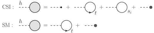
Figure 1: Higgs tadpole diagrams in the CSI model and the SM. A blob in the CSI model represents the tree-level vertex, while a vertex with cross represents the counterterms. (The counterterms in the CSI model and the SM are different. See text.)

In the CSI model, there is a tree-level Higgs tadpole diagram, which contributes $-\xi^{2}\lambda_{\rm H}\mu^{-\epsilon}v^{3}h$, and the singlet and top-quark one-loop diagrams contribute at the same order. To cancel the UV divergence, the counterterm is also needed. In the SM, on the other hand, the tree-level tadpole contributions cancel (since we set $\mu_{H}^{2}=\lambda_{\rm H}^{\rm SM}v^{2}$) at ${\cal O}(\xi^{2})$ and only the counterterms and loop diagrams remain. The corresponding diagrams are shown in Fig. 1. Thus, the conditions for vanishing tadpole contributions read, respectively, as

$${\rm CSI}:~{}~{}\xi^{2}\lambda_{\rm H}+\delta\lambda_{\rm H}=\xi^{2}\frac{N\lambda_{\rm HS}^{2}}{(4\pi)^{2}}\tilde{A}_{0}(\xi m_{s}^{2})-\xi^{2}\frac{N_{c}y_{t}^{4}}{(4\pi)^{2}}\tilde{A}_{0}(\xi m_{t}^{2})\,,$$ (2.11)

$${\rm SM:}~{}~{}-\delta\mu_{\rm H}^{2}/v^{2}+\delta\lambda_{\rm H}^{\rm SM}=-\xi^{2}\frac{N_{c}y_{t}^{4}}{(4\pi)^{2}}\tilde{A}_{0}(\xi m_{t}^{2})\,,$$ (2.12)

at ${\cal O}(\xi^{2})$. Here, the top-quark mass is given by $m_{t}=y_{t}v/\sqrt{2}$, the number of colors $N_{c}=3$, and $\tilde{A}_{0}(m^{2})$ denotes the loop function defined in App. B. Eq. (2.11) coincides with eq. (3.11) of ref. [7] in the case that $\mu=v$ and the counterterm is defined in the $\overline{\rm MS}$ scheme.

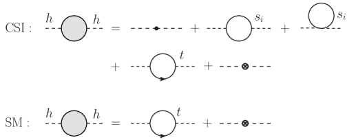
Figure 2: Higgs self-energy diagrams in the CSI model and the SM. Similarly to Fig. 1, a blob and a vertex with a cross represent the tree-level vertex and counterterm, respectively.

We can compute the Higgs self-energy in a similar manner. The corresponding diagrams are shown in Fig. 2, and the results are given by

$${\rm CSI}:~{}~{}$$

$$-\Sigma_{h}(p^{2})=-3(\xi^{2}\lambda_{\rm H}+\delta\lambda_{\rm H})v^{2}+\delta Z_{h}p^{2}+\xi^{2}\frac{N\lambda^{2}_{\rm HS}v^{2}}{(4\pi)^{2}}\left[2B_{0}(p^{2};\xi m_{s}^{2})+\tilde{A}_{0}(\xi m_{s}^{2})\right]$$

$$~{}~{}~{}~{}~{}~{}~{}~{}~{}~{}~{}~{}~{}~{}~{}~{}-\xi^{2}\frac{2N_{c}y_{t}^{2}}{(4\pi)^{2}}\left[\frac{p^{2}}{\xi}B_{1}(p^{2};\xi m_{t}^{2})+2m_{t}^{2}B_{0}(p^{2};\xi m_{t}^{2})+m_{t}^{2}\tilde{A}_{0}(\xi m_{t}^{2})\right]+{\cal O}(\xi^{3})\,,$$ (2.13)

$${\rm SM:}~{}~{}$$

$$-\Sigma_{h}^{\rm SM}(p^{2})=\delta\mu_{\rm H}^{2}-3\delta\lambda_{\rm H}^{\rm SM}v^{2}+\delta Z_{h}^{\rm SM}p^{2}$$

$$~{}~{}~{}~{}~{}~{}~{}~{}~{}~{}~{}~{}~{}~{}~{}~{}~{}-\xi^{2}\frac{2N_{c}y_{t}^{2}}{(4\pi)^{2}}\left[\frac{p^{2}}{\xi}B_{1}(p^{2};\xi m_{t}^{2})+2m_{t}^{2}B_{0}(p^{2};\xi m_{t}^{2})+m_{t}^{2}\tilde{A}_{0}(\xi m_{t}^{2})\right]+{\cal O}(\xi^{3})\,.$$ (2.14)

Here, $B_{i}(p^{2};m^{2})\equiv B_{i}(p^{2};m^{2},m^{2})$ denote the loop functions defined in App. B. We have included the counterterms for the wave function renormalization $\delta Z_{h}p^{2}$, $\delta Z_{h}^{\rm SM}p^{2}$. After the divergence in $B_{1}(p^{2};\xi m_{t}^{2})$ is subtracted by $\delta Z_{h}$, $p^{2}\log(p^{2})$ remains in the self-energy. However, this term is canceled by top-bottom loop in $WWh$ coupling. Taking the $WWh$ correction into account, some finite pieces give corrections to the Higgs propagator. However, they are $O(\xi^{3})$, which is beyond the order of our interest in the following discussion. Hence we neglect them hereafter.

Using the self-energy, the on-shell Higgs mass $m_{h}$ is defined in each model as

$${\rm CSI}:~{}~{}\xi^{2}m_{h}^{2}=\Sigma_{h}(\xi^{2}m_{h}^{2})\,,$$ (2.15)

$${\rm SM}:~{}~{}\xi^{2}m_{h}^{2}=(\xi\,{m_{h,\text{tree}}^{\rm SM}})^{2}+\Sigma_{h}^{\rm SM}(\xi^{2}m_{h}^{2})\,.$$ (2.16)

The tree-level SM Higgs mass $m_{h,\text{tree}}^{\rm SM}$ is defined in eq. (2.7).

For later convenience, we reduce the difference of the Higgs inverse propagators of the two models to a simple form. Combining eqs. (2.11)–(2.16), we obtain

$$-\Delta\Sigma_{h}(p^{2})\equiv ~{}\Bigl{[}p^{2}-\Sigma_{h}(p^{2})\Bigr{]}-\Bigl{[}p^{2}-{(\xi\,{m^{\rm SM}_{h,\text{tree}}})}^{2}-\Sigma_{h}^{\rm SM}(p^{2})\Bigr{]}$$

$$= ~{}\xi^{2}\frac{2N\lambda_{\rm HS}^{2}v^{2}}{(4\pi)^{2}}\left[B_{0}(p^{2};\xi m_{s}^{2})-B_{0}(\xi^{2}m_{h}^{2};\xi m_{s}^{2})\right]\,.$$ (2.17)

Note that the top-loop contributions as well as contributions of the Higgs quartic couplings have dropped from this expression.

Let us focus on the CSI model and examine relations between the parameters of the Lagrangian and physical observables. Substituting eqs. (2.13) and (2.11) into eq. (2.15), we obtain a simple expression for the on-shell Higgs mass as

$$\xi^{2}m_{h}^{2}= -\xi^{2}\frac{2N\lambda^{2}_{\rm HS}v^{2}}{(4\pi)^{2}}\left[B_{0}(\xi^{2}m_{h}^{2};\xi m_{s}^{2})-\tilde{A}_{0}(\xi m_{s}^{2})\right]$$

$$+\xi^{2}\frac{2N_{c}y_{t}^{4}v^{2}}{(4\pi)^{2}}\left[B_{0}(\xi^{2}m_{h}^{2};\xi m_{t}^{2})-\tilde{A}_{0}(\xi m_{t}^{2})\right]\,+{\cal O}(\xi^{3})$$ (2.18)

$$= ~{}\xi^{2}\frac{2N\lambda^{2}_{\rm HS}v^{2}}{(4\pi)^{2}}-\xi^{2}\frac{2N_{c}y_{t}^{4}v^{2}}{(4\pi)^{2}}+{\cal O}(\xi^{3})\,,$$ (2.19)

where in the second equality we used the asymptotic form of the loop function given in App. B, taking into account $\xi^{2}m_{h}^{2}\ll\xi m_{t}^{2},\,\xi m_{s}^{2}$.

Comparing eq. (2.19) with the experimental data, we can determine $\lambda_{\rm HS}$. (It is natural to regard this coupling to be renormalized at scale $\mu\simeq 2m_{s}$.) Using the central values of $m_{h}=125.03\pm 0.27~{}{\rm GeV}$ [18, 19], $v=246.66~{}{\rm GeV}$ and $m_{t}=173.34\pm 0.76~{}{\rm GeV}$ [20], we obtain

$$\lambda_{\rm HS}(\mu\simeq 2m_{s})\approx 4.82/{\sqrt{N}}\,.$$ (2.20)

We also find that the top loop contribution amounts to (only) about $5\%$ in the physical Higgs mass eq. (2.19).

One can also check that the NG bosons become massless by similar calculations.

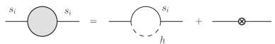
Figure 3: Singlet self-energy diagrams contributing to the lowest-order radiative corrections to the singlet mass $m_{s}$. (Note that $\lambda_{S}$ is omitted throughout the paper.)

The singlet mass is given by eq. (2.5) at tree level. The lowest-order radiative correction is given by the singlet-Higgs one-loop contribution shown in Fig. 3, which is ${\cal O}(\xi^{2})$. Thus, the physical singlet mass is given by

$$\xi m_{s}^{2}=\xi\lambda_{\rm HS}v^{2}+{\cal O}(\xi^{2})\,$$ (2.21)

at the LO. We summarize the values of the parameters in Tab. 2. They agree well with the previous results [7]. We use the values in the table to compute $WW\to WW$ cross sections in the next section.

$N$	1	4	12
$\lambda_{\rm HS}(\mu\simeq 2m_{s})$	4.82	2.41	1.39
$m_{s}$ [GeV]	541	383	291

Table 2: Values of the parameters of the CSI model determined from the VEV and mass of the Higgs boson. They are used in the computation of $WW\to WW$ cross sections.

3 $WW$ scattering processes

In this section we investigate scattering processes of the $W$ bosons. We calculate the amplitudes for the scattering processes $W^{+}W^{-}\rightarrow W^{+}W^{-}$ (Sec. 3.1) and $W^{+}W^{+}\rightarrow W^{+}W^{+}$ (Sec. 3.2). Then we show that in the CSI model the differential cross sections of the longitudinal $W$ boson scattering $W_{L}W_{L}\to W_{L}W_{L}$ deviate from the SM predictions, especially when the energy scale of the scattering processes is much higher than the electroweak scale (Sec. 3.3). In this section we set $\xi=1$ except where we count orders in $\xi$.

3.1 Amplitude for $W^{+}W^{-}\rightarrow W^{+}W^{-}$

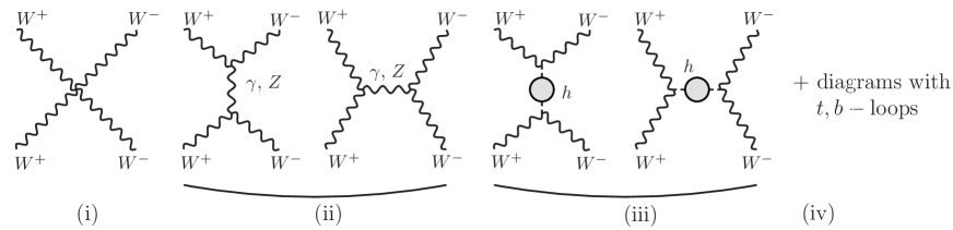
Figure 4: Diagrams for $W^{+}W^{-}\rightarrow W^{+}W^{-}$ scattering. Time flows upwards.

First we calculate the scattering amplitude for $W^{+}W^{-}\rightarrow W^{+}W^{-}$. We consider the following four types of diagrams, shown in Fig. 4: (i) quartic $W$-boson vertex, (ii) $\gamma$- and $Z$-boson exchange diagrams ($s$- and $t$-channels), (iii) Higgs-boson exchange diagrams ($s$- and $t$-channels), and (iv) diagrams including $t$- and $b$-quark loops (up to one loop). The type (i) and (ii) diagrams include only tree diagrams. In the type (iii) diagrams, we include Higgs self-energy, up to ${\cal O}(\xi^{2})$, in the denominator of the Higgs propagator. To avoid double-counting, we eliminate the Higgs self-energy diagram from (iv) . In the case of $W_{L}^{+}W_{L}^{-}\to W_{L}^{+}W_{L}^{-}$ scattering at high energy, these diagrams correspond to the LO [${\cal O}(\xi^{2})$] amplitude for the NG-boson scattering $G^{+}G^{-}\to G^{+}G^{-}$, using the equivalence theorem.

At a first glance, it is not obvious how the above diagrams are related to the couplings of the Higgs sector, as predicted by the equivalence theorem. This is because the couplings of the Higgs sector do not appear explicitly, except in the Higgs self-energy diagrams. As well known, there is a severe gauge cancellation at high energy among the type (i)–(iii) diagrams. After gauge cancellation, the sum of these diagrams behaves proportionally to the Higgs self-interaction, in accord with the equivalence theorem. The type (iv) diagrams are even more subtle. After gauge cancellation, the part proportional to $m_{t}^{4}$ of these diagrams is expected to give order $\xi^{2}y_{t}^{4}/(4\pi)^{2}$ contributions.

The difference of the $W^{+}W^{-}\rightarrow W^{+}W^{-}$ amplitudes between the CSI model and the SM originates from the Higgs exchange diagrams (iii). We express the amplitude in each model as

$${\rm CSI}:~{}~{}{\cal A}_{W^{+}W^{-}\rightarrow W^{+}W^{-}}^{\text{CSI}}={\cal A}^{\rm quart}_{W^{+}W^{-}}+{\cal A}^{\gamma/Z}_{W^{+}W^{-}}+{\cal A}^{h}_{W^{+}W^{-}}+{\cal A}^{t}_{W^{+}W^{-}}\,,$$

$${\rm SM}:~{}~{}{\cal A}_{W^{+}W^{-}\rightarrow W^{+}W^{-}}^{\rm SM}={\cal A}^{\rm quart}_{W^{+}W^{-}}+{\cal A}^{\gamma/Z}_{W^{+}W^{-}}+{\cal A}^{h,{\rm SM}}_{W^{+}W^{-}}+{\cal A}^{t}_{W^{+}W^{-}}\,,$$ (3.1)

where ${\cal A}^{\rm quart}_{W^{+}W^{-}}$, ${\cal A}^{\gamma/Z}_{W^{+}W^{-}}$, ${\cal A}^{h{\rm(,SM)}}_{W^{+}W^{-}}$ and ${\cal A}^{t}_{W^{+}W^{-}}$ represent the sub-amplitudes corresponding to the diagrams (i)–(iv), respectively. ${\cal A}^{\rm quart}_{WW}$, ${\cal A}^{\gamma/Z}_{W^{+}W^{-}}$ and ${\cal A}^{t}_{W^{+}W^{-}}$ are common in both models, whereas ${\cal A}^{h}_{W^{+}W^{-}}$ and ${\cal A}^{h,{\rm SM}}_{W^{+}W^{-}}$ are different. As we have seen in the previous section, the singlet loop gives a LO [${\cal O}(\xi^{2})$] contribution to the Higgs self-energy in the CSI model, which is absent in the SM.

Assigning the momenta of the initial- and final-state particles as $W^{+}(p_{1})W^{-}(p_{2})\rightarrow W^{+}(k_{1})W^{-}(k_{2})$, and setting $s=(p_{1}+p_{2})^{2}$ and $t=(p_{1}-k_{1})^{2}$, we obtain

$${\rm CSI}:~{}~{}{\cal A}^{h}_{W^{+}W^{-}}=-g_{2}^{2}m_{W}^{2}\frac{1}{s-\Sigma_{h}(s)}\ \epsilon(p_{1})\cdot\epsilon^{*}(p_{2})\ \epsilon^{*}(k_{1})\cdot\epsilon(k_{2})$$

$$~{}~{}~{}~{}~{}~{}~{}~{}~{}~{}~{}~{}~{}~{}~{}~{}~{}~{}~{}~{}~{}-g_{2}^{2}m_{W}^{2}\frac{1}{t-\Sigma_{h}(t)}\ \epsilon(p_{1})\cdot\epsilon^{*}(p_{2})\ \epsilon^{*}(k_{1})\cdot\epsilon(k_{2})\,,$$ (3.2)

$${\rm SM}:~{}~{}{\cal A}^{h,{\rm SM}}_{W^{+}W^{-}}=-g_{2}^{2}m_{W}^{2}\frac{1}{s-({m_{h,{\rm tree}}^{\rm SM}})^{2}-\Sigma^{\rm SM}_{h}(s)}\ \epsilon(p_{1})\cdot\epsilon^{*}(p_{2})\ \epsilon^{*}(k_{1})\cdot\epsilon(k_{2})$$

$$~{}~{}~{}~{}~{}~{}~{}~{}~{}~{}~{}~{}~{}~{}~{}~{}~{}~{}~{}~{}~{}~{}-g_{2}^{2}m_{W}^{2}\frac{1}{t-({m_{h,{\rm tree}}^{\rm SM}})^{2}-\Sigma^{\rm SM}_{h}(t)}\ \epsilon(p_{1})\cdot\epsilon^{*}(p_{2})\ \epsilon^{*}(k_{1})\cdot\epsilon(k_{2})\,,$$ (3.3)

where $g_{2}$ and $m_{W}$ represent, respectively, the gauge coupling of $SU(2)_{L}$ and the $W$ boson mass. $\epsilon^{\mu}(p_{i})$, $\epsilon^{\mu}(k_{i})$ represent the polarization vectors of the $W$ bosons characterized by their momenta. The first and second terms of each amplitude correspond to the $s$- and $t$-channel Higgs exchange diagrams, respectively. Thus, the difference of the two amplitudes can be attributed to the difference of the Higgs propagators given by

$$\frac{1}{s-\Sigma_{h}(s)}-\frac{1}{s-{(m_{h,{\rm tree}}^{\rm SM})}^{2}-\Sigma^{\rm SM}_{h}(s)}$$

$$~{}~{}~{}~{}~{}~{}~{}~{}~{}~{}=-\frac{1}{s^{2}}\cdot\frac{2N\lambda_{\rm HS}^{2}v^{2}}{(4\pi)^{2}}\left[B_{0}(s;m_{s}^{2})-B_{0}(m_{h}^{2};m_{s}^{2})\right]+{\cal O}(\xi^{3})\,,$$ (3.4)

and to the corresponding difference for the $t$-channel Higgs propagators. We have used eq. (2.17). Note that ${(m_{h}^{\rm SM})}^{2}$, $\Sigma^{\rm SM}_{h}$, $\Sigma_{h}$ are all ${\cal O}(\xi^{2})$ quantities.

The main purpose of our analysis is to clarify the deviation of the prediction of the CSI model from the SM prediction. We find that the deviation can be taken into account by adding the difference eq. (3.4) to each Higgs propagator in the SM amplitude. Alternatively, one may add $-\Delta\Sigma_{h}(p^{2})$ defined in eq. (2.17) to the denominator of the Higgs propagator in the SM, which is more accurate in kinematical regions close to on-shell Higgs productions. This is one of the main results of this paper. Noting that eq. (3.4) vanishes as $s\to m_{h}^{2}$, we see that indeed an “off-shell Higgs boson” gives clues to the electroweak symmetry breaking mechanism, as anticipated in the Introduction.

Let us check the high energy behavior of the scattering amplitude for $W_{L}^{+}W_{L}^{-}\to W_{L}^{+}W_{L}^{-}$ by comparing to the NG-boson scattering amplitude. At high energy $s,|t|\gg m_{W}^{2}$, the polarization vectors of longitudinal $W$ bosons grow. Consequently, we have

$$\epsilon_{L}(p_{1})\cdot\epsilon_{L}^{*}(p_{2})=\epsilon^{*}_{L}(k_{1})\cdot\epsilon_{L}(k_{2})=\frac{(\beta^{2}+1)s}{4m_{W}^{2}}~{}~{}~{}~{}~{}~{}~{}~{}~{}~{}~{}\to~{}~{}\frac{s}{2m_{W}^{2}}\,,$$ (3.5)

$$\epsilon_{L}(p_{1})\cdot\epsilon^{*}_{L}(k_{1})=\epsilon_{L}^{*}(p_{2})\cdot\epsilon_{L}(k_{2})=\frac{\beta^{2}(\beta^{2}-1)s-2t}{4\beta^{2}m_{W}^{2}}~{}~{}\to~{}~{}\frac{-t}{2m_{W}^{2}}\,.$$ (3.6)

Here, the subscript “$L$” stands for the longitudinal mode; $\beta$ is the velocity of the $W$ bosons in the c.m. frame, i.e., $\beta=\sqrt{1-4m_{W}^{2}/s}$. It follows that, at high energy, $s,|t|\gg m_{s}^{2}$, the difference of the scattering amplitudes behaves as

$${\cal A}_{W^{+}_{L}W^{-}_{L}\rightarrow W^{+}_{L}W^{-}_{L}}^{\text{CSI}}-{\cal A}_{W^{+}_{L}W^{-}_{L}\rightarrow W^{+}_{L}W^{-}_{L}}^{\rm SM}$$

$$~{}~{}~{}\longrightarrow~{}~{}~{}\frac{2N\lambda_{\rm HS}^{2}}{(4\pi)^{2}}\left[B_{0}(s;m_{s}^{2})+B_{0}(t;m_{s}^{2})-2B_{0}(m_{h}^{2};m_{s}^{2})\right]$$

$$~{}~{}~{}~{}~{}~{}~{}~{}~{}~{}~{}~{}~{}\approx\frac{2N\lambda_{\rm HS}^{2}}{(4\pi)^{2}}\left[\log\left(\frac{m_{s}^{4}}{st}\right)+4\right]+{\cal O}\left(\frac{m_{s}^{2}}{s},\frac{m_{s}^{2}}{|t|}\right)\,.$$ (3.7)

This agrees with the difference of the $G^{+}G^{-}\rightarrow G^{+}G^{-}$ amplitudes of the two models, given in eq. (D.8), which is consistent with the equivalence theorem.

3.2 Amplitude for $W^{+}W^{+}\rightarrow W^{+}W^{+}$

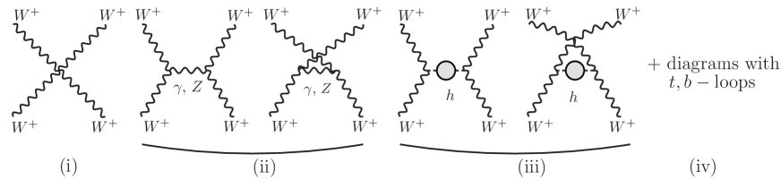
Figure 5: Diagrams for $W^{+}W^{+}\rightarrow W^{+}W^{+}$ scattering. (Time flows upwards, which is similar to Fig. 4.)

It is straightforward to compute the $W^{+}W^{+}\rightarrow W^{+}W^{+}$ scattering process in a similar manner. The diagrams are shown in Fig. 5. The amplitudes for the CSI model and the SM are given by

$${\rm CSI}:~{}~{}{\cal A}_{W^{+}W^{+}\rightarrow W^{+}W^{+}}^{\text{CSI}}={\cal A}^{\rm quart}_{W^{+}W^{+}}+{\cal A}^{\gamma/Z}_{W^{+}W^{+}}+{\cal A}^{h}_{W^{+}W^{+}}+{\cal A}^{t}_{W^{+}W^{+}}\,,$$

$${\rm SM}:~{}~{}{\cal A}_{W^{+}W^{+}\rightarrow W^{+}W^{+}}^{\rm SM}={\cal A}^{\rm quart}_{W^{+}W^{+}}+{\cal A}^{\gamma/Z}_{W^{+}W^{+}}+{\cal A}^{h,{\rm SM}}_{W^{+}W^{+}}+{\cal A}^{t,{\rm SM}}_{W^{+}W^{+}}\,,$$ (3.8)

where the notations are similar to the previous subsection. The Higgs-exchange diagrams are given by

$${\rm CSI}:~{}~{}{\cal A}^{h}_{W^{+}W^{+}}=-g_{2}^{2}m_{W}^{2}\frac{1}{t-\Sigma_{h}(t)}\ \epsilon(p_{1})\cdot\epsilon^{*}(k_{1})\ \epsilon(p_{2})\cdot\epsilon^{*}(k_{2})$$

$$~{}~{}~{}~{}~{}~{}~{}~{}~{}~{}~{}~{}~{}~{}~{}~{}~{}~{}~{}~{}~{}-g_{2}^{2}m_{W}^{2}\frac{1}{u-\Sigma_{h}(u)}\ \epsilon(p_{1})\cdot\epsilon^{*}(k_{2})\ \epsilon(p_{2})\cdot\epsilon^{*}(k_{1})\,,$$

$${\rm SM}:~{}~{}{\cal A}^{h,{\rm SM}}_{W^{+}W^{+}}=-g_{2}^{2}m_{W}^{2}\frac{1}{t-({m_{h,{\rm tree}}^{\rm SM}})^{2}-\Sigma^{\rm SM}_{h}(t)}\ \epsilon(p_{1})\cdot\epsilon^{*}(k_{1})\ \epsilon(p_{2})\cdot\epsilon^{*}(k_{2})$$

$$~{}~{}~{}~{}~{}~{}~{}~{}~{}~{}~{}~{}~{}~{}~{}~{}~{}~{}~{}~{}~{}~{}-g_{2}^{2}m_{W}^{2}\frac{1}{u-({m_{h,{\rm tree}}^{\rm SM}})^{2}-\Sigma^{\rm SM}_{h}(u)}\ \epsilon(p_{1})\cdot\epsilon^{*}(k_{2})\ \epsilon(p_{2})\cdot\epsilon^{*}(k_{1})\,,$$ (3.9)

with $u=(p_{1}-k_{2})^{2}$ for $W^{+}(p_{1})W^{+}(p_{2})\rightarrow W^{+}(k_{1})W^{+}(k_{2})$. Thus, we can calculate the difference of the two amplitudes similarly to the previous subsection.

Using

$$\epsilon_{L}(p_{1})\cdot\epsilon^{*}_{L}(k_{2})=\epsilon_{L}(p_{2})\cdot\epsilon^{*}_{L}(k_{1})=\frac{\beta^{2}(\beta^{2}+1)s+2t}{4\beta^{2}m_{W}^{2}}~{}~{}\to~{}~{}\frac{-u}{2m_{W}^{2}}\,,$$ (3.10)

for $|t|,|u|\gg m_{W}^{2}$, we obtain the high energy behavior of the deviation as

$${\cal A}_{W^{+}_{L}W^{+}_{L}\rightarrow W^{+}_{L}W^{+}_{L}}^{\text{CSI}}-{\cal A}_{W^{+}_{L}W^{+}_{L}\rightarrow W^{+}_{L}W^{+}_{L}}^{\rm SM}$$

$$~{}~{}~{}\longrightarrow\frac{2N\lambda_{\rm HS}^{2}}{(4\pi)^{2}}\left[B_{0}(t;m_{s}^{2})+B_{0}(u;m_{s}^{2})-2B_{0}(m_{h}^{2};m_{s}^{2})\right]$$

$$~{}~{}~{}~{}~{}~{}~{}~{}~{}\approx\frac{2N\lambda_{\rm HS}^{2}}{(4\pi)^{2}}\left[\log\left(\frac{m_{s}^{4}}{tu}\right)+4\right]+{\cal O}\left(\frac{m_{s}^{2}}{s},\frac{m_{s}^{2}}{|t|}\right)\,.$$ (3.11)

As expected, this expression agrees with the corresponding amplitude for $G^{+}G^{+}\rightarrow G^{+}G^{+}$ given in eq. (D.11).

3.3 Cross sections for $W_{L}W_{L}$ scatterings: Numerical study

We perform a numerical study of the $W_{L}W_{L}$ scattering cross sections using the results of the previous subsections. Up to now, we considered (at least formally) all the top-loop corrections which contribute to the LO of $\xi$ expansion at high energy. In the following numerical study, however, we include only those part of the top-loop corrections which are enhanced by logarithms of the energy $\sim\log s,\log|t|$, for the following reason. To the best of our knowledge, the full one-loop electroweak corrections to the $WW$ scattering processes have been presented only numerically for the $W^{+}W^{-}$ scattering in ref. [17] and the analytical formulas are not available. Even only for the $W^{+}W^{-}$ scattering, it is formidable to convert the numerical results given in ref. [17] to our analysis. On the other hand, as we noted in Sec. 2.2, the top-loop contributions are numerically smaller, i.e., of the order of 10%, as compared to the LO contributions by the singlet loops. Hence, the above prescription would be a pragmatic method of computation for this first study. We will further discuss this issue in Sec. 4.

The differential cross sections for $W^{+}_{L}W^{-}_{L}\rightarrow W^{+}_{L}W^{-}_{L}$ and $W^{+}_{L}W^{+}_{L}\rightarrow W^{+}_{L}W^{+}_{L}$ are given by

$$\left[\frac{d\sigma}{d\cos\theta}\right]_{W^{+}_{L}W^{-}_{L}\rightarrow W^{+}_{L}W^{-}_{L}} =\frac{1}{32\pi s}|{\cal A}_{W^{+}_{L}W^{-}_{L}\rightarrow W^{+}_{L}W^{-}_{L}}|^{2}\,,$$ (3.12)

$$\left[\frac{d\sigma}{d\cos\theta}\right]_{W^{+}_{L}W^{+}_{L}\rightarrow W^{+}_{L}W^{+}_{L}} =\frac{1}{64\pi s}|{\cal A}_{W^{+}_{L}W^{+}_{L}\rightarrow W^{+}_{L}W^{+}_{L}}|^{2}\,.$$ (3.13)

Here, $\theta$ is the angle between the initial $W^{+}$ and final $W^{+}$ momenta in the c.m. frame, which satisfies $\cos\theta=\frac{2t}{s\beta^{2}}+1$. We compare the following three cases: (a) SM tree-level cross section, (b) SM LO cross section, and (c) CSI model LO cross section, and for the individual cases the amplitudes in eqs. (3.12) and (3.13) are given by

$${\rm(a):}~{}{\cal A}^{\rm SM}_{\rm tree}={\cal A}^{\rm quart}+{\cal A}^{\gamma/Z}+{\cal A}^{h,{\rm SM}}|_{\rm tree}\,,$$ (3.14)

$${\rm(b):}~{}{\cal A}^{\rm SM}={\cal A}^{\rm quart}+{\cal A}^{\gamma/Z}+{\cal A}^{h,{\rm SM}}\,,$$ (3.15)

$${\rm(c):}~{}{\cal A}^{\rm CSI}={\cal A}^{\rm quart}+{\cal A}^{\gamma/Z}+{\cal A}^{h}\,.$$ (3.16)

Here the subscript “$W^{+}W^{-}$” or “$W^{+}W^{+}$” is suppressed. The formulas for the sub-amplitudes ${\cal A}^{\rm quart}$, ${\cal A}^{\gamma/Z}$, ${\cal A}^{h,\text{SM}}$ are given in App. C. In the Higgs-exchange diagrams only the Higgs propagators are different, i.e., the Higgs propagator is given by

$${\rm(a):}~{}\Delta_{h}^{\text{SM,tree}}=1/(p^{2}-m_{h}^{2})\,,$$ (3.17)

$${\rm(b):}~{}\Delta_{h}^{\text{SM}}=1/(p^{2}-m_{h}^{2}-\Sigma_{h}^{t,\text{log}}(p^{2}))\,,$$ (3.18)

$${\rm(c):}~{}\Delta_{h}^{\text{CSI}}=1/(p^{2}-m_{h}^{2}-\Sigma_{h}^{t,\text{log}}(p^{2})-\Delta\Sigma_{h}(p^{2}))\,,$$ (3.19)

where $\Delta\Sigma_{h}(p^{2})$ is defined in eq. (2.17) and

$$-\Sigma_{h}^{t,\text{log}}(p^{2}) =-\frac{2N_{c}y_{t}^{4}v^{2}}{(4\pi)^{2}}[B_{0}(p^{2};m_{t}^{2})-B_{0}(m_{h}^{2};m_{t}^{2})]\,.$$ (3.20)

It is worth mentioning that close to the pole both $\Delta_{h}^{\rm SM}(p^{2})$ and $\Delta_{h}^{\rm CSI}(p^{2})$ behave as

$$\Delta_{h}^{\text{SM,CSI}}(p^{2})=\frac{1}{p^{2}-m_{h}^{2}}\times\Bigl{[}1+{\cal O}(\xi)\Bigr{]}+(\mbox{regular part as $p^{2}\to m_{h}^{2}$})\,.$$ (3.21)

Hence, they have the correct pole structure at the LO of $\xi$.

Before showing the numerical results it would be useful to see the high energy behavior of ${\cal A}^{\rm SM}$ for comparison with the prediction of the CSI model [c.f., eqs. (3.7) and (3.11)]:

$${\cal A}^{\rm SM}_{W^{+}_{L}W^{-}_{L}\rightarrow W^{+}_{L}W^{-}_{L}}\approx -4\lambda_{\rm H}^{\rm SM}-\frac{g_{Z}^{2}}{2}\left[\frac{s}{t}+\frac{t}{s}+1\right]$$

$$-\frac{2N_{c}y_{t}^{4}}{(4\pi)^{2}}\left[\log\left(\frac{m_{t}^{4}}{st}\right)+\text{const.}\right]+{\cal O}\left(\frac{m_{t}^{2}}{s}\right)\,,$$ (3.22)

$${\cal A}^{\rm SM}_{W^{+}_{L}W^{+}_{L}\rightarrow W^{+}_{L}W^{+}_{L}}\approx -4\lambda_{\rm H}^{\rm SM}-\frac{g_{Z}^{2}}{2}\left[\frac{u}{t}+\frac{t}{u}+1\right]$$

$$-\frac{2N_{c}y_{t}^{4}}{(4\pi)^{2}}\left[\log\left(\frac{m_{t}^{4}}{tu}\right)+\text{const.}\right]+{\cal O}\left(\frac{m_{t}^{2}}{s}\right)\,,$$ (3.23)

where $g_{Z}=\sqrt{g_{Y}^{2}+g_{2}^{2}}$ [$\,g_{Y}$ is the gauge coupling of $U(1)_{Y}$]. The coefficients of the logarithms are consistent with the $y_{t}^{4}$ part of the one-loop beta function of $\lambda_{\rm H}^{\rm SM}$.

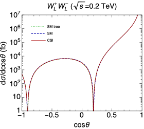
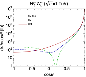
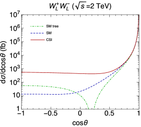
Figure 6: Differential cross sections for $W^{+}_{L}W^{-}_{L}\rightarrow W^{+}_{L}W^{-}_{L}$ process for the c.m. energies $\sqrt{s}=0.2$ TeV, 1 TeV and 2 TeV. We set $N=1$. $\theta$ represents the angle between the initial $W^{+}$ and final $W^{+}$ momenta in the c.m. frame. See text for the input parameters. Dot-dashed (green) line represents the Born SM cross section, dashed (blue) line the SM cross section, and solid (red) line the CSI model cross section.

With the above amplitudes, we compute the cross sections, which are shown in Fig. 6 for the $W^{+}_{L}W^{-}_{L}$ scattering and in Fig. 8 for the $W^{+}_{L}W^{+}_{L}$ scattering. We display the case $N=1$ as an example. The input parameters are taken as $m_{W}=80.385$ GeV, $m_{Z}=91.1876$ GeV ($Z$ boson mass), $m_{h}=125.03$ GeV, $m_{t}=173.34$ GeV, and $g_{2}=0.65178$. Other parameters are derived using the tree-level SM relations: $\sin^{2}\theta_{W}=1-m_{W}^{2}/m_{Z}^{2}$, $v=2m_{W}/g_{2}$, $y_{t}=\sqrt{2}m_{t}/v$. $\lambda_{\rm HS}$ and $m_{s}$ are given in Tab. 2. In $W^{+}_{L}W^{-}_{L}$ scattering (Fig. 6) we see that the deviation [difference of the solid (red) and dashed (blue) lines] is larger at higher energy. The deviation gets prominent at $\sqrt{s}\gtrsim 1$ TeV. Note that the deviation is characteristic to off-shell Higgs bosons as we discussed below eq. (3.4). For instance, at $\cos\theta=0.5$, the CSI model cross section is about 2.3 (1.9) times larger than the SM cross section at $\sqrt{s}=1\,(2)$ TeV.

Nevertheless it might be necessary to observe the deviation at a smaller angle in order to gain statistics. Since the deviation eq. (3.7) includes an enhancement factor $\sim\log|t|$ in the forward region, a priori it is not obvious whether the deviation is highly suppressed in the forward region due to the enhancement of the SM cross section in that region. In fact the deviation is a complicated function of $s$ and $\theta$, and can become relevant. For instance, the CSI model cross section is larger than the SM cross section by 29% (13%) at $\cos\theta=0.8\,(0.9)$ at $\sqrt{s}=1$ TeV. For comparison, in Fig. 7 we plot the ratio of the differential cross sections for the CSI model and the SM as a function of $\cos\theta$ at different c.m. energies.

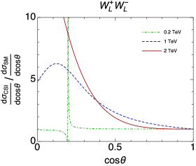
Figure 7: Ratio of the $W^{+}_{L}W^{-}_{L}$ scattering differential cross sections for the CSI model and SM vs. $\cos\theta$, at $\sqrt{s}=0.2$ TeV (green dot-dashed), 1 TeV (blue dashed) and 2 TeV (red solid).

Taken at face value, there is a huge deviation in the backward region $\cos\theta\lesssim 0$ at high energy as can be seen in Fig. 6. In this very kinematical region, however, perturbative convergence of the SM prediction is lost. This can be verified by comparing the Born SM cross section and the LO SM cross section (with only the log-enhanced part of top-loops) in the same figures. More accurately, one can confirm this feature in the full one-loop electroweak corrections computed in ref. [17]. In this kinematical region we need to resum certain IR logarithms to stabilize the SM prediction. Hence, our predictions for the relative size of the deviation with respect to the SM cross section are not reliable at $\cos\theta\lesssim 0.4$, although the size of the deviation itself is well under control.

If we increase $N$, the effective coupling $\sqrt{N}\lambda_{\rm HS}$ of the loop correction is unchanged, while the singlet mass $m_{s}$ becomes smaller. As a result, the deviation tends to get larger. On the other hand, there occurs a cancellation between the singlet contribution and the SM amplitude in some exceptional kinematical points, and the deviation becomes small close to such kinematical points. For example, in the case $N=4$ and $\cos\theta=0.5$, the CSI model cross section is about 3.1 (1.7) times larger than the SM cross section at $\sqrt{s}=1\,(2)$ TeV.

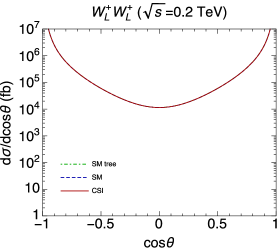
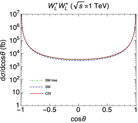
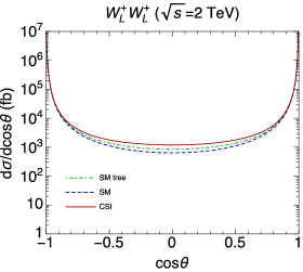
Figure 8: Same as Fig. 6 but for $W^{+}_{L}W^{+}_{L}\rightarrow W^{+}_{L}W^{+}_{L}$ process.

We can make a similar analysis for the $W^{+}_{L}W^{+}_{L}$ scattering cross sections (Fig. 8).

In fact, the $W^{+}_{L}W^{+}_{L}$ scattering channel would be more promising than the $W^{+}_{L}W^{-}_{L}$ channel for detecting the deviation from the SM since the backgrounds, such as $W^{+}_{T}W^{-}_{T}$ contributions, can be reduced effectively [16]. By definition, the $W^{+}_{L}W^{+}_{L}$ differential cross section is symmetric under $\theta\to\pi-\theta$. The cross section exhibits strong enhancement in the forward and backward regions, $\cos\theta\to\pm 1$, due to the $t$- and $u$-channel gauge and Higgs boson exchanges. The deviation of the CSI model prediction from the SM prediction is larger in the central region $\cos\theta\sim 0$ (where the cross section becomes small) and at higher energy. This feature can be seen in the figures. For example, at $\cos\theta=0$, the CSI model cross section is 24% (87%) larger than the SM cross section at $\sqrt{s}=1\,(2)$ TeV. The deviation may also be important in the forward or backward region. The CSI model cross section is larger than the SM cross section by 9% (25%) at $\cos\theta=\pm 0.8$ and by 5% (12%) at $\cos\theta=\pm 0.9$ when $\sqrt{s}=1\,(2)$ TeV. Unlike for the $W^{+}W^{-}$ scattering, the deviation in the forward region is larger at $\sqrt{s}=2$ TeV than at $\sqrt{s}=1$ TeV.

Convergence of the perturbative prediction of the SM cross section is good for the $W^{+}W^{+}$ scattering. Thus in the entire range of $\theta$ and $\sqrt{s}$ analyzed here, we can predict the relative significance of the deviation reliably. In Fig. 9 we show the ratio of the differential cross sections for the CSI model and the SM as a function of $\cos\theta$, at different c.m. energies. If we increase $N$, the deviation becomes larger. Differently from the $W^{+}_{L}W^{-}_{L}$ scattering, there is no cancellation between the singlet contribution and the SM amplitude. The deviation for $N=4$ (as an example) becomes larger than that in $N=1$ case by a factor 1.2–2, depending on $\cos\theta$ and $\sqrt{s}$ shown in the figures.

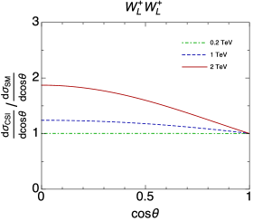
Figure 9: Same as Fig. 7 but for $W^{+}_{L}W^{+}_{L}$ scattering.

For the convenience of the reader, we list values of the scattering amplitudes at some sample kinematical points in Tab. 3. Note that at $\sqrt{s}>2m_{t}$, the amplitudes ${\cal A}^{\text{SM}}$ and ${\cal A}^{\text{CSI}}$ exhibit imaginary part from the self-energy in the $s$-channel Higgs propagator for the $W^{+}W^{-}$ scattering.

Before closing this section, we comment on the Landau pole and perturbative unitarity. One may worry about the validity of the numerical results in this section due to existence of low-scale Landau pole in this model. For $N=1$, it is located at 3.5–4.7 TeV. (It becomes higher for larger $N$, e.g., 16–19 TeV for $N=4$. ) A more well-defined criterion may be given by the unitarity bounds. We have checked that unitarity of the partial wave amplitudes for the $W^{+}_{L}W^{-}_{L}$ and $W^{+}_{L}W^{+}_{L}$ scatterings is violated at $\sqrt{s}\gtrsim 2.8$ TeV if we substitute the one-loop running coupling constants for the renormalized parameters. Therefore our predictions make sense up to slightly below this scale. (In this sense our results at $\sqrt{s}=2$ TeV should be taken with some caution.) On the other hand, it should also be stressed that the breakdown of the perturbative unitarity originates only from the Landau pole and that the theory is well defined perturbatively. This situation is similar to the simple scalar $\phi^{4}$ theory which has a Landau pole. If we adopt a UV completion of our model, such as in ref. [4], there is no Landau pole up to Planck scale and perturbative unitarity is never violated up to this scale.

$W^{+}_{L}W^{-}_{L}$ scattering ($\cos\theta=0.5$)

$\sqrt{s}$ [TeV]	$0.2$	$1$	2
${\cal A}^{\rm CSI}$	$0.722$	$0.729-0.105i$	$0.415+0.661i$
${\cal A}^{\rm SM}$	$0.717$	$0.471-0.109i$	$0.553-0.114i$
${\cal A}^{\rm SM}_{\rm tree}$	$0.724$	$0.393$	$0.379$

$W^{+}_{L}W^{+}_{L}$ scattering ($\cos\theta=0$)

$\sqrt{s}$ [TeV]	$0.2$	$1$	2
${\cal A}^{\rm CSI}$	$-0.487$	$-1.35$	$-1.57$
${\cal A}^{\rm SM}$	$-0.486$	$-1.21$	$-1.15$
${\cal A}^{\rm SM}_{\rm tree}$	$-0.487$	$-1.30$	$-1.33$

Table 3: Values of the amplitudes defined in eqs. (3.14), (3.15), (3.16) for the $N=1$ case. $\cos\theta=0.5$ and $\cos\theta=0$ are chosen for the $W^{+}_{L}W^{-}_{L}$ and $W^{+}_{L}W^{+}_{L}$ scattering processes, respectively.

4 Conclusions and discussion

Although experimental results so far, especially at the LHC, are almost consistent with predictions of the SM, the mechanism of electroweak symmetry breaking has not been completely unveiled yet. Gauge boson scattering is important to understand underlying physics of electroweak symmetry breaking.

Classical scale invariance with extended Higgs sector is an alternative scenario for the electroweak symmetry breaking. We have computed $WW$ scattering cross sections in a minimal model with classical scale invariance (CSI model) as a model of new physics. This model is perturbatively renormalizable and we have developed a theoretical basis necessary for consistent perturbative computation of Feynman amplitudes. This requires a specific assignment of order counting, which is organized in powers of an auxiliary parameter $\xi$.

The deviation of the CSI model predictions from the SM predictions is clarified. It arises from the loop correction by singlet field in the Higgs self-energy and it is incorporated by $\Delta\Sigma_{h}$, defined in eq. (2.17). $\Delta\Sigma_{h}$ characterizes the information on symmetry breaking mechanism carried by an off-shell Higgs boson. The obtained formulas can be used for general $W$ polarizations. We have compared the scattering amplitudes for the longitudinal $W$ bosons ($W_{L}W_{L}\to W_{L}W_{L}$) and NG bosons ($GG\to GG$) and confirmed that they coincide in the high energy limit, which is consistent with the equivalence theorem.

The obtained amplitudes for $WW$ scattering enable us to access the details of the kinematics of the scattering processes, which is impossible from the effective potential (since it is given by zero external momentum limit). This point can be seen by looking at the deviation of the Higgs quartic coupling of the effective potential:

$$\frac{1}{3!}\frac{\partial^{4}}{\partial\phi^{4}} [V_{\text{eff}}^{\text{CSI}}(\phi)-V_{\text{eff}}^{\text{SM}}(\phi)]$$

$$=\frac{1}{3!}\frac{\partial^{4}}{\partial\phi^{4}}\left[\frac{1}{4}\{(\lambda_{\text{H}}+\delta\lambda_{\text{H}})-(\lambda_{\text{H}}^{\text{SM}}+\delta\lambda_{\text{H}}^{\text{SM}})\}\phi^{4}+\frac{N\lambda_{\text{HS}}^{2}}{4(4\pi)^{2}}\phi^{4}\left(\log\frac{\lambda_{\text{HS}}\phi^{2}}{\mu^{2}}-\frac{3}{2}\right)\right]$$

$$=\frac{N\lambda_{\text{HS}}^{2}}{(4\pi)^{2}}\left[\log\frac{\lambda_{\rm HS}\phi^{2}}{m_{s}^{2}}+\frac{8}{3}\right]\,.$$ (4.1)

This should be compared with

$$-\frac{1}{4}\Delta{\cal A}_{W^{+}_{L}W^{-}_{L}\to W^{+}_{L}W^{-}_{L}}~{}\to~{} \frac{N\lambda_{\rm HS}^{2}}{(4\pi)^{2}}\,\left[\log\left(\frac{\sqrt{st}}{m_{s}^{2}}\right)-2\right]\,,$$ (4.2)

$$-\frac{1}{4}\Delta{\cal A}_{W^{+}_{L}W^{+}_{L}\to W^{+}_{L}W^{+}_{L}}~{}\to~{} \frac{N\lambda_{\rm HS}^{2}}{(4\pi)^{2}}\,\left[\log\left(\frac{\sqrt{tu}}{m_{s}^{2}}\right)-2\right]\,,$$ (4.3)

obtained from eqs. (3.7) and (3.11). Comparing them, one could expect the anomalous $\frac{N\lambda_{\rm HS}^{2}}{(4\pi)^{2}}\log s$ behavior of ${\cal A}_{W_{L}W_{L}\to W_{L}W_{L}}$ in the high energy limit from the effective potential if $\phi$ is interpreted as $\sqrt{s}$. However, it is impossible to give the other terms correctly or make predictions for lower energy scattering from the effective potential. From this viewpoint the computation based on the proper order counting using the auxiliary parameter $\xi$ is crucial for the accurate predictions for $WW$ scattering processes.

For $W^{+}_{L}W^{-}_{L}$ scattering we predict +29% (+13%) deviation at, e.g., $\cos\theta=0.8\,(0.9)$ at $\sqrt{s}=1$ TeV with $N=1$. ($\theta$ is the angle between the incident and scattered $W^{+}$ bosons, and the cross section is expected to increase as $\cos\theta\to 1$.) For $W^{+}_{L}W^{+}_{L}$ scattering we may profit from a larger cross section around $\cos\theta\simeq\pm 1$, and a deviation of +25% (+12%) at $\cos\theta=\pm 0.8\,(\pm 0.9)$ and $\sqrt{s}=2$ TeV is predicted. If we increase $N$, the deviation tends to become larger for both cases.

In summary we can describe the characteristic aspects of the CSI model as follows. (1) The deviations in $W_{L}W_{L}$ cross sections are large, and (2) they can be quantified by well-known loop functions.

Finally some remarks for future studies are in order. Our main purpose is to set up a theoretical basis for implementing the predictions of the CSI model to Monte Carlo event generators. We have found a simple prescription to modify the SM predictions, as stated above. This prescription is valid also for off-shell $W$ processes as it is clear from the derivation. In addition, it is independent of gauge choice for the electroweak gauge symmetry since the portal interaction is not affected by the gauge fixing condition. As we checked in Secs. 3.1 and 3.2, it preserves gauge cancellation and satisfies the equivalence theorem [12, 13, 14] for the CSI model. Therefore, the prescription is suited for implementation to Monte Carlo simulation for collider experiments.

It is not trivial whether the model can be tested using $W_{L}W_{L}$ scattering processes at the LHC experiments. According to [16], luminosity of initial $W_{L}$s would not be too suppressed compared to that of $W_{T}$s. Past researches, such as refs. [16, 21], or recent works [22, 23, 24], would be useful for devising kinematical cuts to enhance signal to background ratio in collider searches. Use of $\tau$ final states may help to enhance $W_{L}$ signals. Detailed study will be given elsewhere [25].

Clearly it is important to have accurate predictions of the SM predictions for $WW$ scattering processes at the LHC experiments. Up to now, perturbative QCD corrections are available at the NLO and next-to-next-to-leading order for various kinematical distributions. Full NLO QCD corrections are implemented in Monte Carlo event generators. On the other hand, full NLO electroweak corrections have not been implemented in event generators so far, despite extensive efforts in this direction. (See, e.g., ref. [26] and references therein.)

Among the SM electroweak corrections, phenomenologically electroweak Sudakov logarithms [27] are known to be important in the processes involving high energy $W$ bosons. (See, e.g., ref. [28] and references therein.) We have not incorporated these effects accurately in this study. They will be taken into account carefully when we make a more realistic testability study. We note that, as far as the deviations of the CSI model predictions from the SM predictions are concerned, Sudakov logarithms are irrelevant, so that it does not affect the prescription which we propose.

Appendices

We collect details of the argument and formulas. In App. A, we show the effective expansion parameter of the CSI model and the SM with our specific order counting. In App. B, loop functions are defined. In App. C, sub-amplitudes for $W_{L}W_{L}\to W_{L}W_{L}$ processes are given analytically. In App. D, NG boson scattering amplitudes are computed.

Appendix A Effective expansion parameter

In this appendix we explain the details of the expansion in terms of the parameter $\xi$. We show that the effective expansion parameter is given by eq. (2.10) if we rescale the couplings by eq. (2.9) and expand in $\xi$.

Before the discussion, we note that we are particularly interested in the high energy limit of Feynman amplitudes. For instance, in the $W$ boson scattering cases which we have mainly discussed, we organize a Feynman amplitude in series expansion in the inverse of the c.m. energy, $A(s)=a_{0}s^{0}+a_{1}s^{-1}+a_{2}s^{-2}+\cdots$, due to existence of gauge cancellation. (External lines are taken to be on-shell, and other kinematical parameters such as $s/t$ are taken to be order one.) Then we expand each $a_{n}$ in terms of $\xi$. In the following argument we suppress $s$ for simplicity. We note that the following argument is valid also in the case that external momentum invariants $p_{i}\!\cdot\!p_{j}$ are set equal to either $m_{h}^{2}$, $m_{s}^{2}$ or zero, which correspond to the computations in Sec. 2.

Let us begin by making a consistency check using eqs. (2.11), (2.13), (2.19). In these equations, $\lambda_{\rm H}$, $\lambda_{\rm HS}^{2}/(4\pi)^{2}$ and $y_{t}^{4}/(4\pi)^{2}[\propto y_{t}^{2}m_{t}^{2}/(4\pi)^{2}]$ are treated as the same order quantities, if we take into account the loop factors as well. It is equivalent to treating $\lambda_{\rm H}/(4\pi)^{2}$, $\lambda_{\rm HS}^{2}/(4\pi)^{4}$ and $y_{t}^{4}/(4\pi)^{4}$ as the same order quantities, which is consistent with eq. (2.9). Thus, in the LO analysis in Sec. 2.3, we correctly compare the quantities formally counted as the same order. It is true for the SM as well.

Let us consider the effective action of the CSI model, which is the generating functional of the amputated one-particle irreducible (1PI) Green functions:

$$\Gamma[\varphi(x)]=\sum_{n}\int d^{D}x_{1}\cdots d^{D}x_{n}\,\Gamma^{(n)}_{i_{1},\cdots,i_{n}}(x_{1},\cdots,x_{n})\,\varphi_{i_{1}}(x_{1})\cdots\varphi_{i_{n}}(x_{n}).$$ (A.4)

Here, we consider the effective action in the symmetric phase, and $\varphi$ denotes the collection of all the fields in the model, e.g., $\varphi_{1}=H$, $\varphi_{2}=S_{i}$, $\varphi_{3}=W_{\mu}^{a}$, $\varphi_{4}=\psi_{L}$, etc., but the details are irrelevant in the following argument. Hence, $\Gamma[\varphi(x)]$ is invariant under the SM gauge transformation and the global $O(N)$ transformation $\varphi\to G_{\text{SM}\times O(N)}\,\varphi$.

For simplicity, we concentrate on $\lambda_{\rm H}$ and $\lambda_{\rm HS}$ and neglect all the other couplings. Before we make the rescaling eq. (2.9), the perturbative expansion of each 1PI Green function takes a form

$$\Gamma^{(n)}_{i_{1},\cdots,i_{n}}(x_{1},\cdots,x_{n})= \,\lambda_{\rm H}^{a(n;i_{1},\cdots,i_{n})}\lambda_{\rm HS}^{b(n;i_{1},\cdots,i_{n})}$$

$$\times\sum_{k,m=0}^{\infty}\left[\frac{\lambda_{\rm H}}{(4\pi)^{2}}\right]^{k}\left[\frac{\lambda_{\rm HS}}{(4\pi)^{2}}\right]^{m}\Gamma^{(n,k,m)}_{i_{1},\cdots,i_{n}}(x_{1},\cdots,x_{n}),$$ (A.5)

where the powers of $\lambda_{\rm H}$ and $\lambda_{\rm HS}$ corresponding to the tree-level 1PI Green function are factored out. Namely, $\Gamma^{(n,0,0)}_{i_{1},\cdots,i_{n}}$ denotes the tree-level 1PI Green function for the particles $\varphi_{i_{1}},\cdots,\varphi_{i_{n}}$, while for $k+m>0$, $k+m$ is equal to the number of loops.

After the rescaling eq. (2.9), we have

$$\Gamma^{(n)}_{i_{1},\cdots,i_{n}}(x_{1},\cdots,x_{n}) \,\to\xi^{2a+b}\lambda_{\rm H}^{a}\lambda_{\rm HS}^{b}$$

$$\times\sum_{k,m=0}^{\infty}\xi^{2k+m}\left[\frac{\lambda_{\rm H}^{1/2}}{(4\pi)}\right]^{2k}\left[\frac{\lambda_{\rm HS}}{(4\pi)^{2}}\right]^{m}\Gamma^{(n,k,m)}_{i_{1},\cdots,i_{n}}(x_{1},\cdots,x_{n}).$$ (A.6)

Thus, for each power of $\lambda_{\rm H}^{1/2}/(4\pi)$ or $\lambda_{\rm HS}/(4\pi)^{2}$, the power of $\xi$ is raised by one. This is consistent with eq. (2.10).

In the symmetry broken phase, we replace the fields as $\varphi_{i}\to v_{i}+\delta\varphi_{i}$, where $v_{i}$ is the VEV of $\varphi_{i}$. Then we re-expand the effective action in $\delta\varphi_{i}$, and the expansion coefficients represent the 1PI Green functions of the broken phase. Since we do not assign powers of $\xi$ to $v_{i}$, the relation between the order counting in $\xi$ and in $\lambda_{\rm H}^{1/2}/(4\pi)$ and $\lambda_{\rm HS}/(4\pi)^{2}$ is unchanged from the symmetric phase.

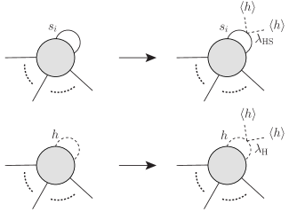
Figure 10: Insertion of $\lambda_{\rm HS}v^{2}s_{i}s_{i}$ vertex to a 1PI diagram, and insertion of $\lambda_{\rm H}v^{2}hh$ vertex to a 1PI diagram, respectively. These manipulations do not increase the number of loops.

The different feature in the broken phase is that one can increase the number of vertices in 1PI diagrams without increasing the number of external legs. For instance, as shown in Fig. 10, we can insert one $\xi\lambda_{\rm HS}$ vertex along the internal singlet line or insert one $\xi^{2}\lambda_{\rm H}$ vertex along the internal Higgs line, together with $v^{2}$. This manipulation does not increase the number of loops, hence the power of $1/(4\pi)^{2}$ does not change. However, the additional dimensionful parameter $v^{2}$ should be compensated by some dimensionful parameter in the denominator, which appears as a result of loop integrals. According to our assumption for the external momentum invariants, this compensation factor, combined with the $v^{2}$, should have a form

$$C=\frac{v^{2}}{\xi m_{s}^{2}}\sum_{n}c_{n}\left(\frac{\xi m_{h}^{2}}{m_{s}^{2}}\right)^{n}\,.$$ (A.7)

Note that

$$\frac{\xi m_{h}^{2}}{m_{s}^{2}}=\xi\frac{\lambda_{\rm HS}}{(4\pi)^{2}}\times\text{const.}+{\cal O}(\xi^{2})\,,$$ (A.8)

$$\frac{v^{2}}{\xi m_{s}^{2}}=\frac{1}{\xi\lambda_{\rm HS}}\times\text{const.}+{\cal O}(\xi^{0})\,,$$ (A.9)

by eqs. (2.19) and (2.21). If we multiply $C$ with the inserted vertex $\xi\lambda_{\rm HS}$ or $\xi^{2}\lambda_{\rm H}=\xi\lambda_{\rm HS}\times[\xi\lambda_{\rm H}^{1/2}/(4\pi)]^{2}\times[\xi\lambda_{\rm HS}/(4\pi)^{2}]^{-1}$, we obtain a series expansion, where $\xi$ is accompanied by each power of $\lambda_{\rm H}^{1/2}/(4\pi)$ or $\lambda_{\rm HS}/(4\pi)^{2}$. In a similar manner, one can verify that inclusion of the VEV of the Higgs field does not change the order counting. Higher powers of $\xi$ on the right-hand side of eqs. (A.8) and (A.9) can be determined iteratively by applying the above method using the terms already determined at lower orders.

By way of example, the one-loop diagram and counterterm in Fig. 3 contribute to the NLO correction to the $\xi$ expansion of the singlet mass as [see eq. (2.21)]

$$\xi m_{s}^{2} =\xi\lambda_{\rm HS}v^{2}+\xi^{2}\frac{\lambda_{\rm HS}^{2}v^{2}}{(4\pi)^{2}}\times\text{const.}$$

$$=\xi\lambda_{\rm HS}v^{2}\left[1+\xi\frac{\lambda_{\rm HS}}{(4\pi)^{2}}\times\text{const.}\right].$$ (A.10)

In the language of the above effective action, the LO term corresponds to $(a,b,k,m)=(0,1,0,0)$, hence $\xi^{2a+b+2k+m}=\xi^{1}$; the NLO term corresponds to $(a,b,k,m)=(0,1,0,1)$, hence $\xi^{2a+b+2k+m}=\xi^{2}$. We can apply this argument including $y_{t}$ or to the case of the SM.

Appendix B Loop functions

We give loop functions in $D=4-2\epsilon$ dimension introducing the renormalization scale $\mu$:

$$\mu^{2\epsilon}\int\frac{d^{D}q}{(2\pi)^{D}}\frac{1}{q^{2}-m^{2}}=\frac{i}{(4\pi)^{2}}m^{2}\tilde{A}_{0}(m^{2})\,,$$ (B.1)

$$\mu^{2\epsilon}\int\frac{d^{D}q}{(2\pi)^{D}}\frac{1}{(q^{2}-m^{2}_{1})((q+p)^{2}-m^{2}_{2})}=\frac{i}{(4\pi)^{2}}B_{0}(p^{2};m^{2}_{1},m^{2}_{2})\,,$$ (B.2)

$$\mu^{2\epsilon}\int\frac{d^{D}q}{(2\pi)^{D}}\frac{q_{\mu}}{(q^{2}-m^{2}_{1})((q+p)^{2}-m^{2}_{2})}=\frac{i}{(4\pi)^{2}}p_{\mu}B_{1}(p^{2};m^{2}_{1},m^{2}_{2})\,.$$ (B.3)

The following expressions are sufficient for our discussion:

$$\tilde{A}_{0}(m^{2})=\frac{1}{\bar{\epsilon}}+\log\left(\frac{\mu^{2}}{m^{2}}\right)+1\,,$$ (B.4)

$$B_{0}(p^{2};m_{1}^{2},m_{2}^{2})=\frac{1}{\bar{\epsilon}}+\log\mu^{2}-\int_{0}^{1}dx\,\log[\,(1-x)m_{1}^{2}+xm_{2}^{2}-x(1-x)p^{2}-i0\,]\,,$$ (B.5)

$$B_{1}(p^{2};m^{2},m^{2})=-\frac{1}{2}B_{0}(p^{2};m^{2},m^{2})\,,$$ (B.6)

with $1/\bar{\epsilon}=1/\epsilon-\gamma+\log 4\pi$ ($\gamma$ is Euler’s number) and

$$B_{0}(p^{2};m^{2})-B_{0}(q^{2};m^{2}) =f(q^{2}/m^{2})-f(p^{2}/m^{2})\,,$$ (B.7)

where

$$f(z) =2+\int_{0}^{1}dx\,\log[\,1-x(1-x)z-i0\,]\rule[-19.91692pt]{0.0pt}{42.67912pt}$$

$$=\left\{\begin{array}[]{llc}\displaystyle\displaystyle 2\sqrt{-d}\,\arctan\biggl{(}\frac{1}{\sqrt{-d}}\biggr{)}\,,&{}{}{}&0<z<4\\ ~{}~{}~{}~{}~{}~{}2\,,&&z=0\\ \displaystyle\sqrt{d}\,\biggl{[}\log\,\biggl{|}\frac{1+\sqrt{d}}{1-\sqrt{d}}\biggr{|}-\pi i\,\theta(z-4)\biggr{]}\,,&{}{}{}&z<0~{}~{}\mbox{or}~{}~{}z\geq 4\end{array}\right.\,,$$ (B.11)

with $d=1-4/z$ and $\theta(x)$ is the step function which is equal to one if $x\geq 0$ and zero if $x<0$. In the text we express $B_{i}(p^{2};m^{2},m^{2})$ as $B_{i}(p^{2};m^{2})$ ($i=0,\,1$) for simplicity.

Asymptotic expressions of $B_{0}(p^{2};m^{2})$ in the limit $|p^{2}|\gg m^{2}$ or $|p^{2}|\ll m^{2}$ are useful:

$$B_{0}(p^{2};m^{2})\xrightarrow{|p^{2}|\gg m^{2}}\frac{1}{\bar{\epsilon}}+\log\left(\frac{\mu^{2}}{-p^{2}}\right)+2+{\cal O}\left(\frac{m^{2}}{|p^{2}|}\right)\,,$$ (B.12)

$$B_{0}(p^{2};m^{2})\xrightarrow{|p^{2}|\ll m^{2}}\frac{1}{\bar{\epsilon}}+\log\left(\frac{\mu^{2}}{m^{2}}\right)+{\cal O}\left(\frac{|p^{2}|}{m^{2}}\right)\,,$$ (B.13)

and for $B_{0}(m^{2};m^{2},m^{\prime 2})$,

$$B_{0}(m^{2};m^{2},m^{\prime 2})\xrightarrow{m^{2}\gg m^{\prime 2}}\frac{1}{\bar{\epsilon}}+\log\left(\frac{\mu^{2}}{m^{2}}\right)+2+{\cal O}\left(\frac{m^{\prime 2}}{m^{2}}\right)\,.$$ (B.14)

Appendix C $W$ boson scattering (in the SM)

Tree-level amplitudes for longitudinally-polarized $W$ boson scattering processes in the standard model are given. The amplitudes for the diagrams (i), (ii) and (iii) in Figs. 4 and 5 are given by

$${\cal A}_{W^{+}_{L}W^{-}_{L}}^{\rm quart} =\frac{g_{2}^{2}}{4m_{W}^{4}\beta^{4}}(t^{2}+st\beta^{2}+3st\beta^{4}+s^{2}\beta^{6})\,,$$ (C.1)

$${\cal A}_{W^{+}_{L}W^{-}_{L}}^{\gamma/Z} =\frac{g_{2}^{2}s^{2}}{16m_{W}^{4}}\left[\frac{\sin^{2}\theta_{W}}{s}+\frac{\cos^{2}\theta_{W}}{s-m_{Z}^{2}}\right]$$

$$~{}~{}~{}\times\left\{-17t+u+2(-4s+7t+u)\beta^{2}+(8s-t+u)\beta^{4}\right\}$$

$$+\frac{g_{2}^{2}}{16m_{W}^{4}\beta^{4}}\left[\frac{\sin^{2}\theta_{W}}{t}+\frac{\cos^{2}\theta_{W}}{t-m_{Z}^{2}}\right]$$

$$~{}~{}~{}\times\bigl{\{}4t^{2}u-s^{3}\beta^{4}(1-\beta^{2})^{2}+s^{2}\beta^{2}(\beta^{2}-1)(4t-(16t+u)\beta^{2}+u\beta^{4})$$

$$~{}~{}~{}~{}~{}-4st(t-(6t+u)\beta^{2}+(6t+u)\beta^{4})\bigr{\}}\,,$$ (C.2)

$${\cal A}_{W^{+}_{L}W^{-}_{L}}^{h,{\rm SM}} =-\frac{g_{2}^{2}}{16m_{W}^{2}\beta^{4}}\left[\frac{s^{2}(1+\beta^{2})^{2}\beta^{4}}{s-{({m^{\rm SM}_{h,\text{tree}}})}^{2}-\Sigma_{h}^{\rm SM}(s)}+\frac{\left\{2t+s\beta^{2}(1-\beta^{2})\right\}^{2}}{t-{({m^{\rm SM}_{h,\text{tree}}})}^{2}-\Sigma_{h}^{\rm SM}(t)}\right]\,,$$

for $W^{+}_{L}W^{-}_{L}\rightarrow W^{+}_{L}W^{-}_{L}$ and

$${\cal A}_{W^{+}_{L}W^{+}_{L}}^{\rm quart} =\frac{g_{2}^{2}}{4m_{W}^{4}\beta^{4}}(-2t^{2}-2st\beta^{2}+s^{2}\beta^{6})\,,$$ (C.4)

$${\cal A}_{W^{+}_{L}W^{+}_{L}}^{\gamma/Z} =\frac{g_{2}^{2}}{16m_{W}^{4}\beta^{4}}\left[\frac{\sin^{2}\theta_{W}}{t}+\frac{\cos^{2}\theta_{W}}{t-m_{Z}^{2}}\right]$$

$$~{}~{}~{}\times\bigl{\{}-4t^{2}u+s^{3}(\beta^{2}-1)^{2}\beta^{4}-s^{2}\beta^{2}(\beta^{2}-1)(4t-(16t+u)\beta^{2}+u\beta^{4})$$

$$~{}~{}~{}~{}+4st(t-(6t+u)\beta^{2}+(6t+u)\beta^{4})\bigr{\}}$$

$$+\frac{g_{2}^{2}}{16m_{W}^{4}\beta^{4}}\left[\frac{\sin^{2}\theta_{W}}{u}+\frac{\cos^{2}\theta_{W}}{u-m_{Z}^{2}}\right]$$

$$~{}~{}~{}\times\bigl{\{}-4t^{3}+s^{3}\beta^{4}(1-3\beta^{2})^{2}+4st^{2}(1-7\beta^{2}+5\beta^{4})$$

$$~{}~{}~{}~{}-s^{2}t\beta^{2}(-4+29\beta^{2}-30\beta^{4}+\beta^{6})\bigr{\}}\,,$$ (C.5)

$${\cal A}_{W^{+}_{L}W^{+}_{L}}^{h,{\rm SM}} =-\frac{g_{2}^{2}}{16m_{W}^{2}\beta^{4}}\left[\frac{\left\{2t+s\beta^{2}(1-\beta^{2})\right\}^{2}}{t-{({m^{\rm SM}_{h,\text{tree}}})}^{2}-\Sigma_{h}^{\rm SM}(t)}+\frac{\left\{2t+s\beta^{2}(1+\beta^{2})\right\}^{2}}{u-{({m^{\rm SM}_{h,\text{tree}}})}^{2}-\Sigma_{h}^{\rm SM}(u)}\right]\,,$$ (C.6)

for $W^{+}_{L}W^{+}_{L}\rightarrow W^{+}_{L}W^{+}_{L}$. These are consistent with the results in refs. [15, 16, 17]

Appendix D Nambu-Goldstone boson scattering

In this section we give the amplitudes for charged NG boson scatterings. According to the equivalence theorem [12, 13, 14], the amplitude for $W^{+}W^{-}\rightarrow W^{+}W^{-}$ ($W^{+}W^{+}\rightarrow W^{+}W^{+}$) should agree with that for $G^{+}G^{-}\rightarrow G^{+}G^{-}$ ($G^{+}G^{+}\rightarrow G^{+}G^{+}$) in the high energy limit. Thus the amplitudes for NG boson scattering can be used for checking the high energy behaviors of the $W$ boson scattering amplitudes, which is especially important to examine the deviations from the SM predictions.

For computation it is useful to rewrite the Higgs quartic coupling and its counterterm in the SM using eqs. (2.11), (2.12), (2.15), and (2.16):

$$\lambda_{\rm H}^{\rm SM}+\delta\lambda_{\rm H}^{\rm SM} =-\frac{N_{c}y_{t}^{4}}{(4\pi)^{2}}\tilde{A}_{0}(m_{t}^{2})-\frac{N\lambda_{\rm HS}^{2}}{(4\pi)^{2}}\left[B_{0}(m_{h}^{2};m_{s}^{2})-\tilde{A}_{0}(m_{s}^{2})\right]+{\cal}O(\xi^{3})\,.$$ (D.1)

Combining with eq. (2.11), we obtain

$$(\lambda_{\rm H}+\delta\lambda_{\rm H})-(\lambda_{\rm H}^{\rm SM}+\delta\lambda_{\rm H}^{\rm SM})=\frac{N\lambda_{\rm HS}^{2}}{(4\pi)^{2}}B_{0}(m_{h}^{2};m_{s}^{2})+{\cal O}(\xi^{3})\,.$$ (D.2)

D.1 $G^{+}G^{-}\rightarrow G^{+}G^{-}$ scattering

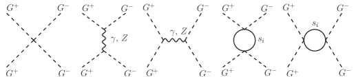
Figure 11: Diagrams for $G^{+}G^{-}\rightarrow G^{+}G^{-}$ scattering. (Time flows upwards.) The last two diagrams are the new contributions in the CSI model.

We derive the amplitude for $G^{+}G^{-}\rightarrow G^{+}G^{-}$ scattering in Landau gauge, which is drawn in Fig. 11. Crucial differences from the SM amplitude reside in the following two points. (a) The Higgs quartic coupling is different (at tree level). (b) The singlet-loop diagram gives non-negligible corrections. We assign momentum of each particle as $G^{+}(p_{1})G^{-}(p_{2})\rightarrow G^{+}(k_{1})G^{-}(k_{2})$, and the results are given by

$${\rm CSI}:~{}~{}{\cal A}^{\rm CSI}_{G^{+}G^{-}\rightarrow G^{+}G^{-}}={\cal A}^{\rm quart}_{G^{+}G^{-}}+{\cal A}^{\gamma/Z}_{G^{+}G^{-}}+{\cal A}^{s}_{G^{+}G^{-}}\,,$$

$${\rm SM}:~{}~{}{\cal A}_{G^{+}G^{-}\rightarrow G^{+}G^{-}}^{\rm SM}={\cal A}^{\rm quart,SM}_{G^{+}G^{-}}+{\cal A}^{\gamma/Z}_{G^{+}G^{-}}\,,$$ (D.3)

where ${\cal A}^{\rm quart}_{G^{+}G^{-}}$, ${\cal A}^{\rm quart,SM}_{G^{+}G^{-}}$ are the quartic vertex, given as

$${\cal A}^{\rm quart}_{G^{+}G^{-}} =-4(\lambda_{\rm H}+\delta\lambda_{\rm H})\,,$$

$${\cal A}^{\rm quart,SM}_{G^{+}G^{-}} =-4(\lambda_{\rm H}^{\rm SM}+\delta\lambda_{\rm H}^{\rm SM})\,,$$ (D.4)

and ${\cal A}^{\gamma/Z}_{G^{+}G^{-}}$ is the tree-level $\gamma$ and $Z$ boson exchange amplitude, which is the same in the CSI and the SM and given by

$${\cal A}^{\gamma/Z}_{G^{+}G^{-}}=-\frac{g_{Z}^{2}}{2}\left[\frac{s}{t}+\frac{t}{s}+1\right]\,.$$ (D.5)

We have neglected the Higgs exchange diagrams since they are suppressed by $1/s$ or $1/t$. Thus we can explicitly see that the tree-level amplitude in the SM,

$${\cal A}_{G^{+}G^{-}\rightarrow G^{+}G^{-}}^{\rm SM}=-4\lambda_{\rm H}^{\rm SM}-\frac{g_{Z}^{2}}{2}\left[\frac{s}{t}+\frac{t}{s}+1\right]\,,$$ (D.6)

agrees with the tree-level amplitude for $W^{+}W^{-}\rightarrow W^{+}W^{-}$ in the high energy limit, i.e., eq. (3.22) without the top-loop contribution.

Finally ${\cal A}^{s}_{G^{+}G^{-}}$ is the contribution of the singlet-loop diagrams, which is given by

$${\cal A}^{s}_{G^{+}G^{-}}=\frac{2N\lambda_{\rm HS}^{2}}{(4\pi)^{2}}\left[B_{0}(s;m_{s}^{2})+B_{0}(t;m_{s}^{2})\right]\,,$$ (D.7)

with $s=(p_{1}+p_{2})^{2}$ and $t=(p_{1}-k_{1})^{2}$. Using eq. (D.2), it is straightforward to obtain

$${\cal A}^{\rm CSI}_{G^{+}G^{-}\rightarrow G^{+}G^{-}}-{\cal A}_{G^{+}G^{-}\rightarrow G^{+}G^{-}}^{\rm SM}=\frac{2N\lambda_{\rm HS}^{2}}{(4\pi)^{2}}\left[B_{0}(s;m_{s}^{2})+B_{0}(t;m_{s}^{2})-2B_{0}(m_{h}^{2};m_{s}^{2})\right]\,.$$ (D.8)

D.2 $G^{+}G^{+}\rightarrow G^{+}G^{+}$ scattering

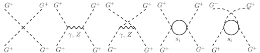
Figure 12: Same as Fig. 11 but for $G^{+}G^{+}\rightarrow G^{+}G^{+}$ scattering.

The same procedure can be used to derive the amplitude for $G^{+}(p_{1})G^{+}(p_{2})\rightarrow G^{+}(k_{1})G^{+}(k_{2})$. The first three diagrams in Fig. 12 give the SM amplitude,

$${\cal A}_{G^{+}G^{+}\rightarrow G^{+}G^{+}}^{\rm SM}=-4\lambda_{\rm H}^{\rm SM}-\frac{g_{Z}^{2}}{2}\left[\frac{u}{t}+\frac{t}{u}+1\right]\,,$$ (D.9)

which is exactly the same as the first two terms of eq. (3.23) as expected. The last two diagrams represent the additional contributions in the CSI model. They are obtained similarly to the $G^{+}G^{-}\rightarrow G^{+}G^{-}$ case:

$${\cal A}^{s}_{G^{+}G^{+}}=\frac{2N\lambda_{\rm HS}^{2}}{(4\pi)^{2}}\left[B_{0}(t;m_{s}^{2})+B_{0}(u;m_{s}^{2})\right]$$ (D.10)

with $u=(p_{1}-k_{2})^{2}$, which leads to

$${\cal A}^{\rm CSI}_{G^{+}G^{+}\rightarrow G^{+}G^{+}}-{\cal A}_{G^{+}G^{+}\rightarrow G^{+}G^{+}}^{\rm SM}=\frac{2N\lambda_{\rm HS}^{2}}{(4\pi)^{2}}\left[B_{0}(t;m_{s}^{2})+B_{0}(u;m_{s}^{2})-2B_{0}(m_{h}^{2};m_{s}^{2})\right]\,.$$ (D.11)

References

- [1] J. R. Espinosa and M. Quiros, Phys. Rev. D 76 (2007) 076004 [hep-ph/0701145].
- [2] R. Foot, A. Kobakhidze and R. R. Volkas, Phys. Lett. B 655 (2007) 156 [arXiv:0704.1165 [hep-ph]].
- [3] L. Alexander-Nunneley and A. Pilaftsis, JHEP 1009 (2010) 021 [arXiv:1006.5916 [hep-ph]].
- [4] D. Chway, T. H. Jung, H. D. Kim and R. Dermisek, Phys. Rev. Lett. 113 (2014) 5, 051801 [arXiv:1308.0891 [hep-ph]].
- [5] O. Antipin, M. Mojaza and F. Sannino, Phys. Rev. D 89 (2014) 8, 085015 [arXiv:1310.0957 [hep-ph]].
- [6] C. Tamarit, Phys. Rev. D 90 (2014) 5, 055024 [arXiv:1404.7673 [hep-ph]].
- [7] K. Endo and Y. Sumino, JHEP 1505, 030 (2015) [arXiv:1503.02819 [hep-ph]].
- [8] S. R. Coleman and E. J. Weinberg, Phys. Rev. D 7 (1973) 1888.
- [9] E. Gildener and S. Weinberg, Phys. Rev. D 13 (1976) 3333.
- [10] K. Hashino, S. Kanemura and Y. Orikasa, Phys. Lett. B 752 (2016) 217 [arXiv:1508.03245 [hep-ph]].
- [11] K. Endo and K. Ishiwata, Phys. Lett. B 749, 583 (2015) [arXiv:1507.01739 [hep-ph]].
- [12] J. M. Cornwall, D. N. Levin and G. Tiktopoulos, Phys. Rev. D 10 (1974) 1145 [Phys. Rev. D 11 (1975) 972].
- [13] C. E. Vayonakis, Lett. Nuovo Cim. 17 (1976) 383.
- [14] M. S. Chanowitz and M. K. Gaillard, Nucl. Phys. B 261 (1985) 379.
- [15] M. J. Duncan, G. L. Kane and W. W. Repko, Nucl. Phys. B 272, 517 (1986).
- [16] V. D. Barger, K. m. Cheung, T. Han and R. J. N. Phillips, Phys. Rev. D 42, 3052 (1990).
- [17] A. Denner and T. Hahn, Nucl. Phys. B 525, 27 (1998) [hep-ph/9711302].
- [18] G. Aad et al. [ATLAS Collaboration], Phys. Rev. D 90, no. 5, 052004 (2014) [arXiv:1406.3827 [hep-ex]].
- [19] V. Khachatryan et al. [CMS Collaboration], Eur. Phys. J. C 74 (2014) 10, 3076 [arXiv:1407.0558 [hep-ex]].
- [20] [ATLAS and CDF and CMS and D0 Collaborations], arXiv:1403.4427 [hep-ex].
- [21] D. A. Dicus, J. F. Gunion and R. Vega, Phys. Lett. B 258, 475 (1991).
- [22] T. Han, D. Krohn, L. T. Wang and W. Zhu, JHEP 1003, 082 (2010) [arXiv:0911.3656 [hep-ph]].
- [23] K. Doroba, J. Kalinowski, J. Kuczmarski, S. Pokorski, J. Rosiek, M. Szleper and S. Tkaczyk, Phys. Rev. D 86, 036011 (2012) [arXiv:1201.2768 [hep-ph]].
- [24] J. M. Campbell and R. K. Ellis, JHEP 1504, 030 (2015) [arXiv:1502.02990 [hep-ph]].
- [25] K. Endo, K. Ishiwata, Y. Shimizu and Y. Sumino in progress.
- [26] S. Gieseke, T. Kasprzik and J. H. Kuhn, Eur. Phys. J. C 74 (2014) 8, 2988 [arXiv:1401.3964 [hep-ph]].
- [27] V. S. Fadin, L. N. Lipatov, A. D. Martin and M. Melles, Phys. Rev. D 61 (2000) 094002 [hep-ph/9910338].
- [28] J. H. Kuhn, F. Metzler, A. A. Penin and S. Uccirati, JHEP 1106 (2011) 143 [arXiv:1101.2563 [hep-ph]].