A Novel Family of Boosted Online Regression Algorithms with Strong Theoretical Bounds

Abstract

We investigate boosted online regression and propose a novel family of regression algorithms with strong theoretical bounds. In addition, we implement several variants of the proposed generic algorithm. We specifically provide theoretical bounds for the performance of our proposed algorithms that hold in a strong mathematical sense. We achieve guaranteed performance improvement over the conventional online regression methods without any statistical assumptions on the desired data or feature vectors. We demonstrate an intrinsic relationship, in terms of boosting, between the adaptive mixture-of-experts and data reuse algorithms. Furthermore, we introduce a boosting algorithm based on random updates that is significantly faster than the conventional boosting methods and other variants of our proposed algorithms while achieving an enhanced performance gain. Hence, the random updates method is specifically applicable to the fast and high dimensional streaming data. Specifically, we investigate Newton Method-based and Stochastic Gradient Descent-based linear regression algorithms in a mixture-of-experts setting, and provide several variants of these well known adaptation methods. However, the proposed algorithms can be extended to other base learners, e.g., nonlinear, tree-based piecewise linear. Furthermore, we provide theoretical bounds for the computational complexity of our proposed algorithms. We demonstrate substantial performance gains in terms of mean square error over the base learners through an extensive set of benchmark real data sets and simulated examples.

1 Introduction

Boosting is considered as one of the most important ensemble learning methods in the machine learning literature and it is extensively used in several different real life applications from classification to regression (Bauer and Kohavi (1999); Dietterich (2000); Schapire and Singer (1999); Schapire and Freund (2012); Freund and E.Schapire (1997); Shrestha and Solomatine (2006); Shalev-Shwartz and Singer (2010); Saigo et al. (2009); Demiriz et al. (2002)). As an ensemble learning method (Fern and Givan (2003); Soltanmohammadi et al. (2016); Duda et al. (2001)), boosting combines several parallel running “weakly” performing algorithms to build a final “strongly” performing algorithm (Soltanmohammadi et al. (2016); Freund (2001); Schapire and Freund (2012); Mannor and Meir (2002)). This is accomplished by finding a linear combination of weak learning algorithms in order to minimize the total loss over a set of training data commonly using a functional gradient descent (Duffy and Helmbold (2002); Freund and E.Schapire (1997)). Boosting is successfully applied to several different problems in the machine learning literature including classification (Jin and Zhang (2007); Chapelle et al. (2011); Freund and E.Schapire (1997)), regression (Duffy and Helmbold (2002); Shrestha and Solomatine (2006)), and prediction (Taieb and Hyndman (2014, 2013)). However, significantly less attention is given to the idea of boosting in online regression framework. To this end, our goal is (a) to introduce a new boosting approach for online regression, (b) derive several different online regression algorithms based on the boosting approach, (c) provide mathematical guarantees for the performance improvements of our algorithms, and (d) demonstrate the intrinsic connections of boosting with the adaptive mixture-of-experts algorithms (Arenas-Garcia et al. (2016); Kozat et al. (2010)) and data reuse algorithms (Shaffer and Williams (1983)).

Although boosting is initially introduced in the batch setting (Freund and E.Schapire (1997)), where algorithms boost themselves over a fixed set of training data, it is later extended to the online setting (Oza and Russell (2001)). In the online setting, however, we neither need nor have access to a fixed set of training data, since the data samples arrive one by one as a stream (Ben-David et al. (1997); Fern and Givan (2003); Lu et al. (2016)). Each newly arriving data sample is processed and then discarded without any storing. The online setting is naturally motivated by many real life applications especially for the ones involving big data, where there may not be enough storage space available or the constraints of the problem require instant processing (Bottou and Bousquet (2008)). Therefore, we concentrate on the online boosting framework and propose several algorithms for online regression tasks. In addition, since our algorithms are online, they can be directly used in adaptive filtering applications to improve the performance of conventional mixture-of-experts methods (Arenas-Garcia et al. (2016)). For adaptive filtering purposes, the online setting is especially important, where the sequentially arriving data is used to adjust the internal parameters of the filter, either to dynamically learn the underlying model or to track the nonstationary data statistics (Arenas-Garcia et al. (2016); Sayed (2003)).

Specifically, we have $m$ parallel running weak learners (WL) (Schapire and Freund (2012)) that receive the input vectors sequentially. Each WL uses an update method, such as the second order Newton’s Method (NM) or Stochastic Gradient Descent (SGD), depending on the target of the applications or problem constraints (Sayed (2003)). After receiving the input vector, each algorithm produces its output and then calculates its instantaneous error after the observation is revealed. In the most generic setting, this estimation/prediction error and the corresponding input vector are then used to update the internal parameters of the algorithm to minimize a priori defined loss function, e.g., instantaneous error for the SGD algorithm. These updates are performed for all of the $m$ WLs in the mixture. However, in the online boosting approaches, these adaptations at each time proceed in rounds from top to bottom, starting from the first WL to the last one to achieve the “boosting” effect (Chen et al. (2012)). Furthermore, unlike the usual mixture approaches (Arenas-Garcia et al. (2016); Kozat et al. (2010)), the update of each WL depends on the previous WLs in the mixture. In particular, at each time $t$, after the $k^{th}$ WL calculates its error over $(\mbox{\boldmath${x}$}_{t},d_{t})$ pair, it passes a certain weight to the next WL, the $(k+1)^{th}$ WL, quantifying how much error the constituent WLs from $1^{st}$ to $k^{th}$ made on the current $(\mbox{\boldmath${x}$}_{t},d_{t})$ pair. Based on the performance of the WLs from $1$ to $k$ on the current $(\mbox{\boldmath${x}$}_{t},d_{t})$ pair, the $(k+1)^{th}$ WL may give a different emphasis (importance weight) to $(\mbox{\boldmath${x}$}_{t},d_{t})$ pair in its adaptation in order to rectify the mistake of the previous WLs.

The proposed idea for online boosting is clearly related to the adaptive mixture-of-experts algorithms widely used in the machine learning literature, where several parallel running adaptive algorithms are combined to improve the performance. In the mixture methods, the performance improvement is achieved due to the diversity provided by using several different adaptive algorithms each having a different view or advantage (Kozat et al. (2010)). This diversity is exploited to yield a final combined algorithm, which achieves a performance better than any of the algorithms in the mixture. Although the online boosting approach is similar to mixture approaches (Kozat et al. (2010)), there are significant differences. In the online boosting notion, the parallel running algorithms are not independent, i.e., one deliberately introduces the diversity by updating the WLs one by one from the first WL to the $m^{th}$ WL for each new sample based on the performance of all the previous WLs on this sample. In this sense, each adaptive algorithm, say the $(k+1)^{th}$ WL, receives feedback from the previous WLs, i.e., $1^{st}$ to $k^{th}$, and updates its inner parameters accordingly. As an example, if the current $(\mbox{\boldmath${x}$}_{t},d_{t})$ is well modeled by the previous WLs, then the $(k+1)^{th}$ WL performs minor update using $(\mbox{\boldmath${x}$}_{t},d_{t})$ and may give more emphasis (importance weight) to the later arriving samples that may be worse modeled by the previous WLs. Thus, by boosting, each adaptive algorithm in the mixture can concentrate on different parts of the input and output pairs achieving diversity and significantly improving the gain.

The linear online learning algorithms, such as SGD or NM, are among the simplest as well as the most widely used regression algorithms in the real-life applications (Sayed (2003)). Therefore, we use such algorithms as base WLs in our boosting algorithms. To this end, we first apply the boosting notion to several parallel running linear NM-based WLs and introduce three different approaches to use the importance weights (Chen et al. (2012)), namely “weighted updates”,“data reuse”, and “random updates”. In the first approach, we use the importance weights directly to produce certain weighted NM algorithms. In the second approach, we use the importance weights to construct data reuse adaptive algorithms (Oza and Russell (2001)). However, data reuse in boosting, such as (Oza and Russell (2001)), is significantly different from the usual data reusing approaches in adaptive filtering (Shaffer and Williams (1983)). As an example, in boosting, the importance weight coming from the $k^{th}$ WL determines the data reuse amount in the $(k+1)^{th}$ WL, i.e., it is not used for the $k^{th}$ filter, hence, achieving the diversity. The third approach uses the importance weights to decide whether to update the constituent WLs or not, based on a random number generated from a Bernoulli distribution with the parameter equal to the weight. The latter method can be effectively used for big data processing (Malik (2013)) due to the reduced complexity. The output of the constituent WLs is also combined using a linear mixture algorithm to construct the final output. We then update the final combination algorithm using the SGD algorithm (Kozat et al. (2010)). Furthermore, we extend the boosting idea to parallel running linear SGD-based algorithm similar to the NM case.

We start our discussions by investigating the related works in Section 2. We then introduce the problem setup and background in Section 3, where we provide individual sequence as well as MSE convergence results for the NM and SGD algorithms. We introduce our generic boosted online regression algorithm in Section 4 and provide the mathematical justifications for its performance. Then, in Sections 5 and 6, three different variants of the proposed boosting algorithm are derived, using the NM and SGD, respectively. Then, in Section 7 we provide the mathematical analysis for the computational complexity of the proposed algorithms. The paper concludes with extensive sets of experiments over the well known benchmark data sets and simulation models widely used in the machine learning literature to demonstrate the significant gains achieved by the boosting notion.

2 Related Works

AdaBoost is one of the earliest and most popular boosting methods, which has been used for binary and multiclass classifications as well as regression (Freund and E.Schapire (1997)). This algorithm has been well studied and has clear theoretical guarantees, and its excellent performance is explained rigorously (Breiman (1997)). However, AdaBoost cannot perform well on the noisy data sets (Servedio (2003)), therefore, other boosting methods have been suggested that are more robust against noise.

In order to reduce the effect of noise, SmoothBoost was introduced in (Servedio (2003)) in a batch setting. Moreover, in (Servedio (2003)) the author proves the termination time of the SmoothBoost algorithm by simultaneously obtaining upper and lower bounds on the weighted advantage of all samples over all of the weak learners. We note that the SmoothBoost algorithm avoids overemphasizing the noisy samples, hence, provides robustness against noise. In (Oza and Russell (2001)), the authors extend bagging and boosting methods to an online setting, where they use a Poisson sampling process to approximate the reweighting algorithm. However, the online boosting method in (Oza and Russell (2001)) corresponds to AdaBoost, which is susceptible to noise. In (Babenko et al. (2009)), the authors use a greedy optimization approach to develop the boosting notion to the online setting and introduce stochastic boosting. Nevertheless, while most of the online boosting algorithms in the literature seek to approximate AdaBoost, (Chen et al. (2012)) investigates the inherent difference between batch and online learning, extend the SmoothBoost algorithm to an online setting, and provide the mathematical guarantees for their algorithm. (Chen et al. (2012)) points out that the online weak learners do not need to perform well on all possible distributions of data, instead, they have to perform well only with respect to smoother distributions. Recently, in (Beygelzimer et al. (2015b)) the authors have developed two online boosting algorithms for classification, an optimal algorithm in terms of the number of weak learners, and also an adaptive algorithm using the potential functions and boost-by-majority (Freund (1995)).

In addition to the classification task, the boosting approach has also been developed for the regression (Duffy and Helmbold (2002)). In (Bertoni et al. (1997)), a boosting algorithm for regression is proposed, which is an extension of Adaboost.R (Bertoni et al. (1997)). Moreover, in (Duffy and Helmbold (2002)), several gradient descent algorithms are presented, and some bounds on their performances are provided. In (Babenko et al. (2009)) the authors present a family of boosting algorithms for online regression through greedy minimization of a loss function. Also, in (Beygelzimer et al. (2015a)) the authors propose an online gradient boosting algorithm for regression.

In this paper we propose a novel family of boosted online algorithms for the regression task using the “online boosting” notion introduced in (Chen et al. (2012)), and investigate three different variants of the introduced algorithm. Furthermore, we show that our algorithm can achieve a desired mean squared error (MSE), given a sufficient amount of data and a sufficient number of weak learners. In addition, we use similar techniques to (Servedio (2003)) to prove the correctness of our algorithm. We emphasize that our algorithm has a guaranteed performance in an individual sequence manner, i.e., without any statistical assumptions on the data. In establishing our algorithm and its justifications, we refrain from changing the regression problem to the classification problem, unlike the AdaBoost.R (Freund and E.Schapire (1997)). Furthermore, unlike the online SmoothBoost (Chen et al. (2012)), our algorithm can learn the guaranteed MSE of the weak learners, which in turn improves its adaptivity.

3 Problem Description and Background

All vectors are column vectors and represented by bold lower case letters. Matrices are represented by bold upper case letters. For a vector ${a}$ (or a matrix ${A}$), $\mbox{\boldmath${a}$}^{T}$ (or $\mbox{\boldmath${A}$}^{T}$) is the transpose and Tr(${A}$) is the trace of the matrix ${A}$. Here, $\mbox{\boldmath${I}$}_{m}$ and $\mbox{\boldmath${0}$}_{m}$ represent the identity matrix of dimension $m\times m$ and the all zeros vector of length $m$, respectively. Except $\mbox{\boldmath${I}$}_{m}$ and $\mbox{\boldmath${0}$}_{m}$, the time index is given in the subscript, i.e., $x_{t}$ is the sample at time $t$. We work with real data for notational simplicity. We denote the mean of a random variable $x$ as $E[x]$. Also, we show the cardinality of a set $S$ by $|S|$.

We sequentially receive $r$-dimensional input (regressor) vectors $\{\mbox{\boldmath${x}$}_{t}\}_{t\geq 1}$, $\mbox{\boldmath${x}$}_{t}\in{\mathbbm{R}}^{r}$, and desired data $\{d_{t}\}_{t\geq 1}$, and estimate $d_{t}$ by $\hat{d}_{t}=f_{t}(\mbox{$\mbox{\boldmath${x}$}$}_{t})$, where $f_{t}(.)$ is an online regression algorithm. At each time $t$ the estimation error is given by $e_{t}=d_{t}-\hat{d}_{t}$ and is used to update the parameters of the WL. For presentation purposes, we assume that $d_{t}\in[-1,1]$, however, our derivations hold for any bounded but arbitrary desired data sequences. In our framework, we do not use any statistical assumptions on the input feature vectors or on the desired data such that our results are guaranteed to hold in an individual sequence manner (Kozat and Singer (Jan. 2008)).

The linear methods are considered as the simplest online modeling or learning algorithms, which estimate the desired data $d_{t}$ by a linear model as $\hat{d}_{t}=\mbox{\boldmath${w}$}_{t}^{T}\mbox{$\mbox{\boldmath${x}$}$}_{t}$, where $\mbox{\boldmath${w}$}_{t}$ is the linear algorithm’s coefficients at time $t$. Note that the previous expression also covers the affine model if one includes a constant term in $\mbox{\boldmath${x}$}_{t}$, hence we use the purely linear form for notational simplicity. When the true $d_{t}$ is revealed, the algorithm updates its coefficients $\mbox{\boldmath${w}$}_{t}$ based on the error $e_{t}$. As an example, in the basic implementation of the NM algorithm, the coefficients are selected to minimize the accumulated squared regression error up to time $t-1$ as

$$\mbox{\boldmath${w}$}_{t} =\arg\min_{\mbox{\boldmath${w}$}}\sum_{l=1}^{t-1}(d_{l}-\mbox{\boldmath${x}$}_{l}^{T}\mbox{\boldmath${w}$})^{2},$$

$$=\left(\sum_{l=1}^{t-1}\mbox{\boldmath${x}$}_{l}\mbox{\boldmath${x}$}_{l}^{T}\right)^{-1}\left(\sum_{l=1}^{t-1}\mbox{\boldmath${x}$}_{l}d_{l}\right),$$ (1)

where ${w}$ is a fixed vector of coefficients. The NM algorithm is shown to enjoy several optimality properties under different statistical settings (Sayed (2003)). Apart from these results and more related to the framework of this paper, the NM algorithm is also shown to be rate optimal in an individual sequence manner (Merhav and Feder (1993)). As shown in (Merhav and Feder (1993)) (Section V), when applied to any sequence $\{\mbox{\boldmath${x}$}_{t}\}_{t\geq 1}$ and $\{d_{t}\}_{t\geq 1}$, the accumulated squared error of the NM algorithm is as small as the accumulated squared error of the best batch least squares (LS) method that is directly optimized for these realizations of the sequences, i.e., for all $T$, $\{\mbox{\boldmath${x}$}_{t}\}_{t\geq 1}$ and $\{d_{t}\}_{t\geq 1}$, the NM achieves

$$\sum_{l=1}^{T}(d_{l}-\mbox{\boldmath${x}$}_{l}^{T}\mbox{\boldmath${w}$}_{l})^{2}-\min_{\mbox{\boldmath${w}$}}\sum_{l=1}^{T}(d_{l}-\mbox{\boldmath${x}$}_{l}^{T}\mbox{\boldmath${w}$})^{2}\leq O(\ln T).$$ (2)

The NM algorithm is a member of the Follow-the-Leader type algorithms (Cesa-Bianchi and Lugosi (2006)) (Section 3), where one uses the best performing linear model up to time $t-1$ to predict $d_{t}$. Hence, (2) follows by direct application of the online convex optimization results (Shalev-Shwartz (2012)) after regularization. The convergence rate (or the rate of the regret) of the NM algorithm is also shown to be optimal so that $O(\ln T)$ in the upper bound cannot be improved (Singer et al. (2002)). It is also shown in (Singer et al. (2002)) that one can reach the optimal upper bound (with exact scaling terms) by using a slightly modified version of (1)

$$\mbox{\boldmath${w}$}_{t}=\left(\sum_{l=1}^{t}\mbox{\boldmath${x}$}_{l}\mbox{\boldmath${x}$}_{l}^{T}\right)^{-1}\left(\sum_{l=1}^{t-1}\mbox{\boldmath${x}$}_{l}d_{l}\right).$$ (3)

Note that the extension (3) of (1) is a forward algorithm (Section 5 of Azoury and Warmuth (2001)) and one can show that, in the scalar case, the predictions of (3) are always bounded (which is not the case for (1)) (Singer et al. (2002)).

We emphasize that in the basic application of the NM algorithm, all data pairs $(d_{l},\mbox{\boldmath${x}$}_{l})$, $l=1,\ldots,t$, receive the same “importance” or weight in (1). Although there exists exponentially weighted or windowed versions of the basic NM algorithm (Sayed (2003)), these methods weight (or concentrate on) the most recent samples for better modeling of the nonstationarity (Sayed (2003)). However, in the boosting framework (Freund and E.Schapire (1997)), each sample pair receives a different weight based on not only those weighting schemes, but also the performance of the boosted algorithms on this pair. As an example, if a WL performs worse on a sample, the next WL concentrates more on this example to better rectify this mistake. In the following sections, we use this notion to derive different boosted online regression algorithms.

Although in this paper we use linear WLs for the sake of notational simplicity, one can readily extend our approach to nonlinear and piecewise linear regression methods. For example, one can use tree based online regression methods (Khan et al. (2016); Vanli and Kozat (2014); Kozat et al. (2007)) as the weak learners, and boost them with the proposed approach.

4 New Boosted Online Regression Algorithm

In this section we present the generic form of our proposed algorithms and provide the guaranteed performance bounds for that. Regarding the notion of “online boosting” introduced in (Chen et al. (2012)), the online weak learners need to perform well only over smooth distributions of data points. We first present the generic algorithm in Algorithm (1) and provide its theoretical justifications, then discuss about its structure and the intuition behind it.

Algorithm 1 Boosted online regression algorithm

1:  Input: $(\mbox{\boldmath${x}$}_{t},d_{t})$ (data stream), $m$ (number of weak learners running in parallel), $\sigma_{m}^{2}$ (the modified desired MSE), and $\sigma^{2}$ (the guaranteed achievable weighted MSE).

2:  Initialize the regression coefficients $\mbox{\boldmath${w}$}_{1}^{(k)}$ for each WL; and the combination coefficients as $\mbox{\boldmath${z}$}_{1}=\frac{1}{m}[1,1,\ldots,1]^{T}$;

3:  for $t=1$ to $T$ do

4:     Receive the regressor data instance $\mbox{\boldmath${x}$}_{t}$;

5:     Compute the WLs outputs $\hat{d}_{t}^{(k)}$;

6:     Produce the final estimate $\hat{d}_{t}=\mbox{\boldmath${z}$}_{t}^{T}\mbox{\boldmath${y}$}_{t}=\mbox{\boldmath${z}$}_{t}^{T}[\hat{d}_{t}^{(1)},\ldots,\hat{d}_{t}^{(m)}]^{T}$;

7:     Receive the true output $d_{t}$ (desired data);

8:     $\lambda_{t}^{(1)}=1$; $l_{t}^{(1)}=0$;

9:     for $k=1$ to $m$ do

10:        $\lambda_{t}^{(k)}=\min\left\{1,\left(\sigma^{2}\right)^{\;l_{t}^{(k)}/2}\right\}$;

11:        Update the WL^(k), such that it has a weighted MSE $\leq\sigma^{2}$;

12:        $e_{t}^{(k)}=d_{t}-\hat{d}_{t}^{(k)}$;

13:        $l_{t}^{(k+1)}=l_{t}^{(k)}+\left[\sigma^{2}_{m}-\left(e_{t}^{(k)}\right)^{2}\right]$;

14:     end for

15:     Update $\mbox{\boldmath${z}$}_{t}$ based on $e_{t}=d_{t}-\mbox{\boldmath${z}$}_{t}^{T}\mbox{\boldmath${y}$}_{t}$;

16:  end for

In Algorithm 1, we have $m$ copies of an online WL, each of which is guaranteed to have a weighted MSE of at most $\sigma^{2}$. We prove that the Algorithm 1 can reach a desired MSE, $\sigma_{d}^{2}$, through Lemma 1, Lemma 2, and Theorem 1. Note that since we assume $d_{t}\in[-1,1]$, the trivial solution $\hat{d}_{t}=0$ incurs an MSE of at most $1$. Therefore, we define a weak learner as an algorithm which has an MSE less than $1$.

Lemma 1. In Algorithm 1, if there is an integer $M$ such that $\sum_{t=1}^{T}\lambda_{t}^{(k)}\geq\kappa T$ for every $k\leq M$, and also $\sum_{t=1}^{T}\lambda_{t}^{(M+1)}<\kappa T$, where $0<\kappa<\sigma_{d}^{2}$ is arbitrarily chosen, it can reach a desired MSE, $\sigma_{d}^{2}$.
Proof. The proof of Lemma 1 is given in Appendix A.

Lemma 2. If the weak learners are guaranteed to have a weighted MSE less than $\sigma^{2}$, i.e.,

$$\forall k:\qquad\frac{\sum_{t=1}^{T}\lambda_{t}^{(k)}(e_{t}^{(k)})^{2}}{4\sum_{t=1}^{T}\lambda_{t}^{(k)}}\leq\sigma^{2}\leq\frac{1}{4},$$

there is an integer $M$ that satisfies the conditions in Lemma 1.

Proof. The proof of Lemma 2 is given in Appendix B.

Theorem 1. If the weak learners in line 11 of Algorithm 1 achieve a weighted MSE of at most $\sigma^{2}<\frac{1}{4}$ , there exists an upper bound for $m$ such that the algorithm reaches the desired MSE.
Proof. This theorem is a direct consequence of combining Lemma 1 and Lemma 2.

Note that although we are using copies of a base learner as the weak learners and seek to improve its performance, the constituent WLs can be different. However, by using the boosting approach, we can improve the MSE performance of the overall system as long as the WLs can provide a weighted MSE of at most $\sigma^{2}$. For example, we can improve the performance of mixture-of-experts algorithms (Arenas-Garcia et al. (2016)) by leveraging the boosting approach introduced in this paper.

As shown in Fig. 1, at each iteration $t$, we have $m$ parallel running WLs with estimating functions $f_{t}^{(k)}$, producing estimates $\hat{d}_{t}^{(k)}=f_{t}^{(k)}(\mbox{\boldmath${x}$}_{t})$ of $d_{t}$, $k=1,\ldots,m$. As an example, if we use $m$ “linear” algorithms, $\hat{d}_{t}^{(k)}=\mbox{\boldmath${x}$}_{t}^{T}\mbox{\boldmath${w}$}_{t}^{(k)}$ is the estimate generated by the $k^{th}$ WL. The outputs of these $m$ WLs are then combined using the linear weights $\mbox{\boldmath${z}$}_{t}$ to produce the final estimate as $\hat{d}_{t}=\mbox{\boldmath${z}$}_{t}^{T}\mbox{\boldmath${y}$}_{t}$ (Kozat et al. (2010)), where $\mbox{\boldmath${y}$}_{t}\triangleq[\hat{d}_{t}^{(1)},\ldots,\hat{d}_{t}^{(m)}]^{T}$ is the vector of outputs. After the desired output $d_{t}$ is revealed, the $m$ parallel running WLs will be updated for the next iteration. Moreover, the linear combination coefficients $\mbox{\boldmath${z}$}_{t}$ are also updated using the normalized SGD (Sayed (2003)), as detailed later in Section 4.1.

Figure 1: The block diagram of a boosted online regression system that uses the input vector $\mbox{\boldmath${x}$}_{t}$ to produce the final estimate $\hat{d}_{t}$. There are $m$ constituent WLs $f_{t}^{(1)},\ldots,f_{t}^{(m)}$, each of which is an online linear algorithm that generates its own estimate $\hat{d}_{t}^{(k)}$. The final estimate $\hat{d}_{t}$ is a linear combination of the estimates generated by all these constituent WLs, with the combination weights $z_{t}^{(k)}$’s corresponding to $\hat{d}_{t}^{(k)}$’s. The combination weights are stored in a vector which is updated after each iteration $t$. At time $t$ the $k^{th}$ WL is updated based on the values of $\lambda_{t}^{(k)}$ and $e_{t}^{(k)}$, and provides the $(k+1)^{th}$ filter with $l_{t}^{(k+1)}$ that is used to compute $\lambda_{t}^{(k+1)}$. The parameter $\delta_{t}^{(k)}$ indicates the weighted MSE of the $k^{th}$ WL over the first $t$ estimations, and is used in computing $\lambda_{t}^{(k)}$.

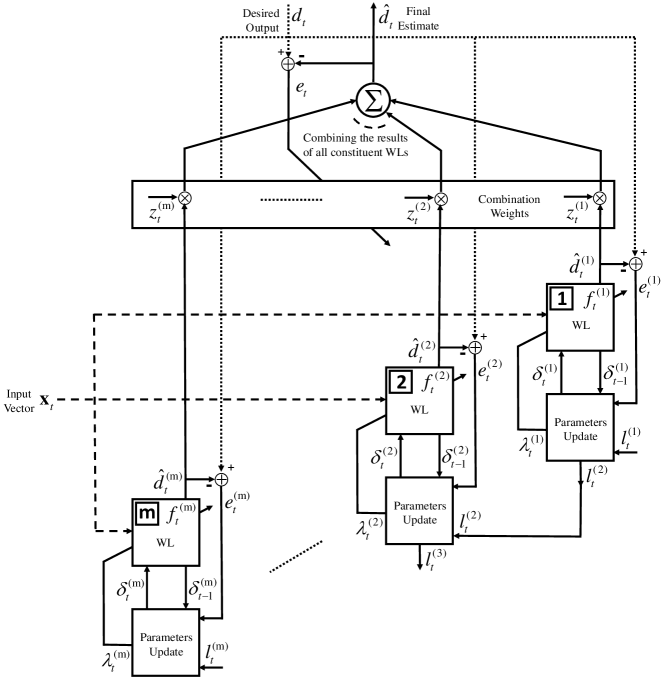
After $d_{t}$ is revealed, the constituent WLs, $f_{t}^{(k)}$, $k=1,\ldots,m$, are consecutively updated, as shown in Fig. 1, from top to bottom, i.e., first $k=1$ is updated, then, $k=2$ and finally $k=m$ is updated. However, to enhance the performance, we use a boosted updating approach (Freund and E.Schapire (1997)), such that the $(k+1)^{th}$ WL receives a “total loss” parameter, $l_{t}^{(k+1)}$, from the $k^{th}$ WL, as

$$l_{t}^{(k+1)}=l_{t}^{(k)}+\left[\sigma_{m}^{2}-\left(d_{t}-f_{t}^{(k)}(\mbox{$\mbox{\boldmath${x}$}$}_{t})\right)^{2}\right],$$ (4)

to compute a weight $\lambda_{t}^{(k)}$. The total loss parameter $l_{t}^{(k)}$, indicates the sum of the differences between the modified desired MSE ($\sigma_{m}^{2}$) and the squared error of the first $k-1$ WLs at time $t$. Then, we add the difference $\sigma_{m}^{2}-(e_{t}^{(k)})^{2}$ to $l_{t}^{(k)}$, to generate $l_{t}^{(k+1)}$, and pass $l_{t}^{(k+1)}$ to the next WL, as shown in Fig. 1. Here, $\left[\sigma_{m}^{2}-\left(d_{t}-f_{t}^{(k)}(\mbox{$\mbox{\boldmath${x}$}$}_{t})\right)^{2}\right]$ measures how much the $k^{th}$ WL is off with respect to the final MSE performance goal. For example, in a stationary environment, if $d_{t}=f(\mbox{$\mbox{\boldmath${x}$}$}_{t})+\nu_{t}$, where $f(\cdot)$ is a deterministic function and $\nu_{t}$ is the observation noise, one can select the desired MSE $\sigma_{d}^{2}$ as an upper bound on the variance of the noise process $\nu_{t}$, and define a modified desired MSE as $\sigma_{m}^{2}\triangleq\frac{\sigma_{d}^{2}-\kappa}{1-\kappa}$. In this sense, $l_{t}^{(k)}$ measures how the WLs $j=1,\ldots,k$ are cumulatively performing on $(d_{t},\mbox{\boldmath${x}$}_{t})$ pair with respect to the final performance goal.

We then use the weight $\lambda_{t}^{(k)}$ to update the $k^{th}$ WL with the “weighted updates”, “data reuse”, or “random updates” method, which we explain later in Sections 5 and 6. Our aim is to make $\lambda_{t}^{(k)}$ large if the first $k-1$ WLs made large errors on $d_{t}$, so that the $k^{th}$ WL gives more importance to $(\mbox{\boldmath${x}$}_{t},d_{t})$ in order to rectify the performance of the overall system. We now explain how to construct these weights, such that $0<\lambda_{t}^{(k)}\leq 1$. To this end, we set $\lambda_{t}^{(1)}=1$, for all $t$, and introduce a weighting similar to (Servedio (2003); Chen et al. (2012)). We define the weights as

$$\lambda_{t}^{(k)}=\min\left\{1,\left(\sigma^{2}\right)^{l_{t}^{(k)}/2}\right\},$$ (5)

where $\sigma^{2}$ is the guaranteed upper bound on the weighted MSE of the weak learners. However, since there is no prior information about the exact MSE performance of the weak learners, we use the following weighting scheme

$$\lambda_{t}^{(k)}=\min\left\{1,\left(\delta_{t-1}^{(k)}\right)^{c\;l_{t}^{(k)}}\right\},$$ (6)

where $\delta_{t-1}^{(k)}$ indicates an estimate of the $k^{th}$ weak learner’s MSE, and $c\geq 0$ is a design parameter, which determines the “dependence” of each WL update on the performance of the previous WLs, i.e., $c=0$ corresponds to “independent” updates, like the ordinary combination of the WLs in adaptive filtering (Kozat et al. (2010); Arenas-Garcia et al. (2016)), while a greater $c$ indicates the greater effect of the previous WLs performance on the weight $\lambda_{t}^{(k)}$ of the current WL. Note that including the parameter $c$ does not change the validity of our proofs, since one can take $\left(\delta_{t-1}^{(k)}\right)^{2c}$ as the new guaranteed weighted MSE. Here, $\delta_{t-1}^{(k)}$ is an estimate of the “Weighted Mean Squared Error” (WMSE) of the $k^{th}$ WL over $\{\mbox{\boldmath${x}$}_{t}\}_{t\geq 1}$ and $\{d_{t}\}_{t\geq 1}$. In the basic implementation of the online boosting (Servedio (2003); Chen et al. (2012)), $\left(1-\delta_{t-1}^{(k)}\right)$ is set to the classification advantage of the weak learners (Servedio (2003)), where this advantage is assumed to be the same for all weak learners. In this paper, to avoid using any a priori knowledge and to be completely adaptive, we choose $\delta_{t-1}^{(k)}$ as the weighted and thresholded MSE of the $k^{th}$ WL up to time $t-1$ as

$$\delta_{t}^{(k)} =\frac{\ {\sum}_{\tau=1}^{t}\frac{\lambda_{\tau}^{(k)}}{4}\left(d_{\tau}-\left[f_{\tau}^{(k)}(\mbox{$\mbox{\boldmath${x}$}$}_{\tau})\right]^{+}\right)^{2}}{\sum_{\tau=1}^{t}\lambda_{\tau}^{(k)}}$$

$$=\frac{\Lambda_{t-1}^{(k)}\delta_{t-1}^{(k)}+\frac{\lambda_{t}^{(k)}}{4}\left(d_{t}-\left[f_{t}^{(k)}(\mbox{$\mbox{\boldmath${x}$}$}_{t})\right]^{+}\right)^{2}}{\Lambda_{t-1}^{(k)}+\lambda_{t}^{(k)}},$$ (7)

where $\Lambda_{t}^{(k)}\triangleq\sum_{\tau=1}^{t}\lambda_{\tau}^{(k)}$, and $\left[f_{\tau}^{(k)}(\mbox{$\mbox{\boldmath${x}$}$}_{\tau})\right]^{+}$ thresholds $f_{\tau}^{(k)}(\mbox{$\mbox{\boldmath${x}$}$}_{\tau})$ into the range $[-1,1]$. This thresholding is necessary to assure that $0<\delta_{t}^{(k)}\leq 1$, which guarantees $0<\lambda_{t}^{(k)}\leq 1$ for all $k=1,\ldots,m$ and $t$. We point out that (7) can be recursively calculated.

Regarding the definition of $\lambda_{t}^{(k)}$, if the first $k$ WLs are “good”, we will pass less weight to the next WLs, such that those WLs can concentrate more on the other samples. Hence, the WLs can increase the diversity by concentrating on different parts of the data Kozat et al. (2010). Furthermore, following this idea, in (6), the weight $\lambda_{t}^{(k)}$ is larger, i.e., close to 1, if most of the WLs, $1,\ldots,k-1$, have errors larger than $\sigma_{m}^{2}$ on $(\mbox{\boldmath${x}$}_{t},d_{t})$, and smaller, i.e., close to 0, if the pair $(\mbox{\boldmath${x}$}_{t},d_{t})$ is easily modeled by the previous WLs such that the WLs $k,\ldots,m$ do not need to concentrate more on this pair.

4.1 The Combination Algorithm

Although in the proof of our algorithm, we assume a constant combination vector ${z}$ over time, we use a time varying combination vector in practice, since there is no knowledge about the exact number of the required week learners for each problem. Hence, after $d_{t}$ is revealed, we also update the final combination weights $\mbox{\boldmath${z}$}_{t}$ based on the final output $\hat{d}_{t}=\mbox{\boldmath${z}$}_{t}^{T}\mbox{\boldmath${y}$}_{t}$, where $\hat{d}_{t}=\mbox{\boldmath${z}$}_{t}^{T}\mbox{\boldmath${y}$}_{t}$, $\mbox{\boldmath${y}$}_{t}=[\hat{d}_{t}^{(1)},\ldots,\hat{d}_{t}^{(m)}]^{T}$. To update the final combination weights, we use the normalized SGD algorithm Sayed (2003) yielding

$$\mbox{\boldmath${z}$}_{t+1}=\mbox{\boldmath${z}$}_{t}+\mu_{z}e_{t}\frac{\mbox{\boldmath${y}$}_{t}}{\|\mbox{\boldmath${y}$}_{t}\|^{2}}.$$ (8)

4.2 Choice of Parameter Values

The choice of $\sigma_{m}^{2}$ is a crucial task, i.e., we cannot reach any desired MSE for any data sequence unconditionally. As an example, suppose that the data are generated randomly according to a known distribution, while they are contaminated with a white noise process. It is clear that we cannot obtain an MSE level below the noise power. However, if the WLs are guaranteed to satisfy the conditions of Theorem 1, this would not happen. Intuitively, there is a guaranteed upper bound (i.e., $\sigma^{2}$) on the worst case performance, since in the weighted MSE, the samples with a higher error have a more important effect. On the other hand, if one chooses a $\sigma_{m}^{2}$ smaller than the noise power, $l_{t}^{(k)}$ will be negative for almost every $k$, turning most of the weights into 1, and as a result the weak learners fail to reach a weighted MSE smaller than $\sigma^{2}$. Nevertheless, in practice we have to choose the parameter $\sigma_{m}^{2}$ reasonably and precisely such that the conditions of Theorem 1 are satisfied. For instance, we set $\sigma_{m}^{2}$ to be an upper bound on the noise power.

In addition, the number of weak learners, $m$, is chosen regarding to the computational complexity constraints. However, in our experiments we choose a moderate number of weak learners, $m=20$, which successfully improves the performance. Moreover, according to the results in Section 8.3, the optimum value for $c$ is around 1, hence, we set the parameter $c=1$ in our simulations.

5 Boosted NM Algorithms

At each time $t$, all of the WLs (shown in Fig. 1) estimate the desired data $d_{t}$ in parallel, and the final estimate is a linear combination of the results generated by the WLs. When the $k^{th}$ WL receives the weight $\lambda_{t}^{(k)}$, it updates the linear coefficients $\mbox{\boldmath${w}$}_{t}^{(k)}$ using one of the following methods.

5.1 Directly Using $\lambda$’s as Sample Weights

Here, we consider $\lambda_{t}^{(k)}$ as the weight for the observation pair $(\mbox{\boldmath${x}$}_{t},d_{t})$ and apply a weighted NM update to $\mbox{\boldmath${w}$}_{t}^{(k)}$. For this particular weighted NM algorithm, we define the Hessian matrix and the gradient vector as

$$\mbox{\boldmath${R}$}_{t+1}^{(k)}\triangleq\beta\mbox{\boldmath${R}$}_{t}^{(k)}+\lambda_{t}^{(k)}\mbox{\boldmath${x}$}_{t}\mbox{\boldmath${x}$}_{t}^{T},$$ (9)

$$\mbox{\boldmath${p}$}_{t+1}^{(k)}\triangleq\beta\mbox{\boldmath${p}$}_{t}^{(k)}+\lambda_{t}^{(k)}\mbox{\boldmath${x}$}_{t}d_{t},$$ (10)

where $\beta$ is the forgetting factor Sayed (2003) and $\mbox{\boldmath${w}$}_{t+1}^{(k)}=\left(\mbox{\boldmath${R}$}_{t+1}^{(k)}\right)^{-1}\mbox{\boldmath${p}$}_{t+1}^{(k)}$ can be calculated in a recursive manner as

$$e_{t}^{(k)}=d_{t}-\mbox{\boldmath${x}$}_{t}^{T}\mbox{\boldmath${w}$}_{t}^{(k)},$$

$$\mbox{\boldmath${g}$}_{t}^{(k)}=\frac{\lambda_{t}^{(k)}\mbox{\boldmath${P}$}_{t}^{(k)}\mbox{\boldmath${x}$}_{t}}{\beta+\lambda_{t}^{(k)}\mbox{$\mbox{\boldmath${x}$}$}_{t}^{T}\mbox{\boldmath${P}$}_{t}^{(k)}\mbox{\boldmath${x}$}_{t}},$$

$$\mbox{\boldmath${w}$}_{t+1}^{(k)}=\mbox{\boldmath${w}$}_{t}^{(k)}+e_{t}^{(k)}\mbox{\boldmath${g}$}_{t}^{(k)},$$

$$\mbox{\boldmath${P}$}_{t+1}^{(k)}=\beta^{-1}\left(\mbox{\boldmath${P}$}_{t}^{(k)}-\mbox{\boldmath${g}$}_{t}^{(k)}\mbox{\boldmath${x}$}_{t}^{T}\mbox{\boldmath${P}$}_{t}^{(k)}\right).$$ (11)

where $\mbox{\boldmath${P}$}_{t}^{(k)}\triangleq\big{(}\mbox{\boldmath${R}$}_{t}^{(k)}\big{)}^{-1}$, and $\mbox{\boldmath${P}$}_{0}^{(k)}=v^{-1}\mbox{\boldmath${I}$}$, and $0<v\ll 1$. The complete algorithm is given in Algorithm 2 with the weighted NM implementation in (11).

Algorithm 2 Boosted NM-based algorithm

1:  Input: $(\mbox{\boldmath${x}$}_{t},d_{t})$ (data stream), $m$ (number of WLs) and $\sigma_{m}^{2}$.

2:  Initialize the regression coefficients $\mbox{\boldmath${w}$}_{1}^{(k)}$ for each WL; and the combination coefficients as $\mbox{\boldmath${z}$}_{1}=\frac{1}{m}[1,1,\ldots,1]^{T}$; and for all $k$ set $\delta_{0}^{(k)}=0$.

3:  for $t=1$ to $T$ do

4:     Receive the regressor data instance $\mbox{\boldmath${x}$}_{t}$;

5:     Compute the WLs outputs $\hat{d}_{t}^{(k)}=\mbox{\boldmath${x}$}_{t}^{T}\mbox{\boldmath${w}$}_{t}^{(k)}$;

6:     Produce the final estimate $\hat{d}_{t}=\mbox{\boldmath${z}$}_{t}^{T}[\hat{d}_{t}^{(1)},\ldots,\hat{d}_{t}^{(m)}]^{T}$;

7:     Receive the true output $d_{t}$ (desired data);

8:     $\lambda_{t}^{(1)}=1$; $l_{t}^{(1)}=0$;

9:     for $k=1$ to $m$ do

10:        $\lambda_{t}^{(k)}=\min\left\{1,\left(\delta_{t-1}^{(k)}\right)^{c\;l_{t}^{(k)}}\right\}$;

11:        Update the regression coefficients $\mbox{\boldmath${w}$}_{t}^{(k)}$ by using the NM and the weight $\lambda_{t}^{(k)}$ based on one of the introduced algorithms in Section 5;

12:        $e_{t}^{(k)}=d_{t}-\hat{d}_{t}^{(k)}$;

13:        $\delta_{t}^{(k)}=\frac{\Lambda_{t-1}^{(k)}\delta_{t-1}^{(k)}+\frac{\lambda_{t}^{(k)}}{4}\left(d_{t}-\left[f_{t}^{(k)}(\mbox{$\mbox{\boldmath${x}$}$}_{t})\right]^{+}\right)^{2}}{\Lambda_{t-1}^{(k)}+\lambda_{t}^{(k)}}$;

14:        $\Lambda_{t}^{(k)}=\Lambda_{t-1}^{(k)}+\lambda_{t}^{(k)}$

15:        $l_{t}^{(k+1)}=l_{t}^{(k)}+\left[\sigma_{m}^{2}-\left(e_{t}^{(k)}\right)^{2}\right]$;

16:     end for

17:     $e_{t}=d_{t}-\mbox{\boldmath${z}$}_{t}^{T}\mbox{\boldmath${y}$}_{t}$;

18:     $\mbox{\boldmath${z}$}_{t+1}=\mbox{\boldmath${z}$}_{t}+\mu_{z}e_{t}\frac{\mbox{\boldmath${y}$}_{t}}{\|\mbox{\boldmath${y}$}_{t}\|^{2}}$;

19:  end for

5.2 Data Reuse Approaches Based on The Weights

Another approach follows Ozaboost (Oza and Russell (2001)). In this approach, from $\lambda_{t}^{(k)}$, we generate an integer, say $n_{t}^{(k)}=\mathrm{ceil}(K\lambda_{t}^{(k)})$, where $K$ is a design parameter that takes on positive integer values. We then apply the NM update on the $(\mbox{\boldmath${x}$}_{t},d_{t})$ pair repeatedly $n_{t}^{(k)}$ times, i.e., run the NM update on the same $(\mbox{\boldmath${x}$}_{t},d_{t})$ pair $n_{t}^{(k)}$ times consecutively. Note that $K$ should be determined according to the computational complexity constraints. However, increasing $K$ does not necessarily result in a better performance, therefore, we use moderate values for $K$, e.g., we use $K=5$ in our simulations. The final $\mbox{\boldmath${w}$}_{t+1}^{(k)}$ is calculated after $n_{t}^{(k)}$ NM updates. As a major advantage, clearly, this reusing approach can be readily generalized to other adaptive algorithms in a straightforward manner.

We point out that Ozaboost (Oza and Russell (2001)) uses a different data reuse strategy. In this approach, $\lambda_{t}^{(k)}$ is used as the parameter of a Poisson distribution and an integer $n_{t}^{(k)}$ is randomly generated from this Poisson distribution. One then applies the NM update $n_{t}^{(k)}$ times.

5.3 Random Updates Approach Based on The Weights

In this approach, we simply use the weight $\lambda_{t}^{(k)}$ as a probability of updating the $k^{th}$ WL at time $t$. To this end, we generate a Bernoulli random variable, which is $1$ with probability $\lambda_{t}^{(k)}$ and is $0$ with probability $1-\lambda_{t}^{(k)}$. Then, we update the $k^{th}$ WL, only if the Bernoulli random variable equals $1$. With this method, we significantly reduce the computational complexity of the algorithm. Moreover, due to the dependence of this Bernoulli random variable on the performance of the previous constituent WLs, this method does not degrade the MSE performance, while offering a considerably lower complexity, i.e., when the MSE is low, there is no need for further updates, hence, the probability of an update is low, while this probability is larger when the MSE is high.

6 Boosted SGD Algorithms

In this case, as shown in Fig. 1, we have $m$ parallel running WLs, each of which is updated using the SGD algorithm. Based on the weights given in (6) and the total loss and MSE parameters in (4) and (7), we next introduce three SGD based boosting algorithms, similar to those introduced in Section 5.

6.1 Directly Using $\lambda$’s to Scale The Learning Rates

We note that by construction method in (6), $0<\lambda_{t}^{(k)}\leq 1$, thus, these weights can be directly used to scale the learning rates for the SGD updates. When the $k^{th}$ WL receives the weight $\lambda_{t}^{(k)}$, it updates its coefficients $\mbox{\boldmath${w}$}_{t}^{(k)}$, as

$$\mbox{\boldmath${w}$}_{t+1}^{(k)}=\left(\mbox{\boldmath${I}$}-\mu^{(k)}\lambda_{t}^{(k)}\mbox{\boldmath${x}$}_{t}\mbox{\boldmath${x}$}_{t}^{T}\right)\mbox{\boldmath${w}$}_{t}^{(k)}+\mu^{(k)}\lambda_{t}^{(k)}\mbox{\boldmath${x}$}_{t}d_{t},$$ (12)

where $0<\mu^{(k)}\lambda_{t}^{(k)}\leq\mu^{(k)}$. Note that we can choose $\mu^{(k)}=\mu$ for all $k$, since the online algorithms work consecutively from top to bottom, and the $k^{th}$ WL will have a different learning rate $\mu^{(k)}\lambda_{t}^{(k)}$.

6.2 A Data Reuse Approach Based on The Weights

In this scenario, for updating $\mbox{\boldmath${w}$}_{t}^{(k)}$, we use the SGD update $n_{t}^{(k)}=\mathrm{ceil}(K\lambda_{t}^{(k)})$ times to obtain the $\mbox{\boldmath${w}$}_{t+1}^{(k)}$ as

$$\mbox{\boldmath${q}$}^{(0)}=\mbox{\boldmath${w}$}_{t}^{(k)},$$

$$\mbox{\boldmath${q}$}^{(a)}=\left(\mbox{\boldmath${I}$}-\mu^{(k)}\mbox{\boldmath${x}$}_{t}\mbox{\boldmath${x}$}_{t}^{T}\right)\mbox{\boldmath${q}$}^{(a-1)}+\mu^{(k)}\mbox{\boldmath${x}$}_{t}d_{t},\;a=1,\ldots,n_{t}^{(k)},$$

$$\mbox{\boldmath${w}$}_{t+1}^{(k)}=\mbox{\boldmath${q}$}^{\left(n_{t}^{(k)}\right)}.$$ (13)

where $K$ is a constant design parameter.

Similar to the NM case, if we follow the Ozaboost (Oza and Russell (2001)), we use the weights to generate a random number $n_{t}^{(k)}$ from a Poisson distribution with parameter $\lambda_{t}^{(k)}$, and perform the SGD update $n_{t}^{(k)}$ times on $\mbox{\boldmath${w}$}_{t}^{(k)}$ as explained above.

6.3 Random Updates Based on The Weights

Again, in this scenario, similar to the NM case, we use the weight $\lambda_{t}^{(k)}$ to generate a random number from a Bernoulli distribution, which equals $1$ with probability $\lambda_{t}^{(k)}$, and equals $0$ with probability $1-\lambda_{t}^{(k)}$. Then we update $\mbox{\boldmath${w}$}_{t}$ using SGD only if the generated number is $1$.

7 Analysis Of The Proposed Algorithms

In this section we provide the complexity analysis for the proposed algorithms. We prove an upper bound for the weights $\lambda_{t}^{(k)}$, which is significantly less than 1. This bound shows that the complexity of the “random updates” algorithm is significantly less than the other proposed algorithms, and slightly greater than that of a single WL. Hence, it shows the considerable advantage of “boosting with random updates” in processing of high dimensional data.

7.1 Complexity Analysis

Here we compare the complexity of the proposed algorithms and find an upper bound for the computational complexity of random updates scenario (introduced in Section 5.3 for NM, and in Section 6.3 for SGD updates), which shows its significantly lower computational burden with respect to two other approaches. For $\mbox{\boldmath${x}$}_{t}\in\mathbbm{R}^{r}$, each WL performs $O(r)$ computations to generates its estimate, and if updated using the NM algorithm, requires $O(r^{2})$ computations due to updating the matrix $\mathbf{R}_{t}^{(k)}$, while it needs $O(r)$ computations when updated using the SGD method (in their most basic implementation).

We first derive the computational complexity of using the NM updates in different boosting scenarios. Since there are a total of $m$ WLs, all of which are updated in the “weighted updates” method, this method has a computational cost of order $O(mr^{2})$ per each iteration $t$. However, in the “random updates”, at iteration $t$, the $k^{th}$ WL may or may not be updated with probabilities $\lambda_{t}^{(k)}$ and $1-\lambda_{t}^{(k)}$ respectively, yielding

$$C_{t}^{(k)}=\begin{cases}O(r^{2})&\quad\text{with probability}\ \lambda_{t}^{(k)}\\ O(r)&\quad\text{with probability}\ 1-\lambda_{t}^{(k)},\end{cases}$$ (14)

where $C_{t}^{(k)}$ indicates the complexity of running the $k^{th}$ WL at iteration $t$. Therefore, the total computational complexity $C_{t}$ at iteration $t$ will be $C_{t}=\sum_{k=1}^{m}C_{t}^{(k)}$, which yields

$$E\left[C_{t}\right]=E\left[\sum_{k=1}^{m}C_{t}^{(k)}\right]=\sum_{k=1}^{m}E[\lambda_{t}^{(k)}]O(r^{2})$$ (15)

Hence, if $E\big{[}\lambda_{t}^{(k)}\big{]}$ is upper bounded by $\tilde{\lambda}^{(k)}<1$, the average computational complexity of the random updates method, will be

$$E\left[C_{t}\right]<\sum_{k=1}^{m}\tilde{\lambda}^{(k)}O(r^{2}).$$ (16)

In Theorem 2, we provide sufficient constraints to have such an upper bound.

Furthermore, we can use such a bound for the “data reuse” mode as well. In this case, for each WL $f_{t}^{(k)}$, we perform the NM update $\lambda_{t}^{(k)}K$ times, resulting a computational complexity of order $\displaystyle E\left[C_{t}\right]<\sum_{k=1}^{m}K\ \tilde{\lambda}^{(k)}(O(r^{2}))$. For the SGD updates, we similarly obtain the computational complexities $O(mr)$, $\sum_{k=1}^{m}O\big{(}\tilde{\lambda}^{(k)}r\big{)}$, and $\sum_{k=1}^{m}O\big{(}K\tilde{\lambda}^{(k)}r\big{)}$, for the “weighted updates”, “random updates”, and “data reuse” scenarios respectively.

The following theorem determines the upper bound $\tilde{\lambda}^{(k)}$ for $E\big{[}\lambda_{t}^{(k)}\big{]}$.
Theorem 2. If the WLs converge and achieve a sufficiently small MSE (according to the proof following this Theorem), the following upper bound is obtained for $\lambda_{t}^{(k)}$, given that $\sigma_{m}^{2}$ is chosen properly,

$$E\left[\lambda_{t}^{(k)}\right]\leq\tilde{\lambda}^{(k)}=\left(\gamma^{-2\sigma_{m}^{2}}(1+2\zeta^{2}\ln\gamma)\right)^{\frac{1-k}{2}},\\$$ (17)

where $\gamma\triangleq E\left[\delta_{t-1}^{(k)}\right]$ and $\zeta^{2}\triangleq E\left[\left(e_{t}^{(k)}\right)^{2}\right]$.
It can be straightforwardly shown that, this bound is less than $1$ for appropriate choices of $\sigma_{m}^{2}$, and reasonable values for the MSE according to the proof. This theorem states that if we adjust $\sigma_{m}^{2}$ such that it is achievable, i.e., the WLs can provide a slightly lower MSE than $\sigma_{m}^{2}$, the probability of updating the WLs in the random updates scenario will decrease. This is of course our desired results, since if the WLs are performing sufficiently well, there is no need for additional updates. Moreover, if $\sigma_{m}^{2}$ is opted such that the WLs cannot achieve a MSE equal to $\sigma_{m}^{2}$, the WLs have to be updated at each iteration, which increases the complexity.

Proof: For simplicity, in this proof, we have assumed that $c=1$, however, the results are readily extended to the general values of $c$. We construct our proof based on the following assumption:
Assumption: assume that $e_{t}^{(k)}$’s are independent and identically distributed (i.i.d) zero-mean Gaussian random variables with variance $\zeta^{2}$.
We have

$$E\left[\lambda_{t}^{(k)}\right] =E\left[\min\left\{1,\left(\delta_{t-1}^{(k)}\right)^{l_{t}^{(k)}}\right\}\right]$$

$$\leq\min\left\{1,E\left[\left(\delta_{t-1}^{(k)}\right)^{l_{t}^{(k)}}\right]\right\}$$ (18)

Now, we show that under certain conditions, $E\big{[}\big{(}\delta_{t-1}^{(k)}\big{)}^{\l_{t}^{(k)}}\big{]}$ will be less than 1, hence, we obtain an upper bound for $E\big{[}\lambda_{t}^{(k)}\big{]}$. We define $s\triangleq\ln(\delta_{t-1}^{(k)})$, yielding

$$E\left[\left(\delta_{t-1}^{(k)}\right)^{\l_{t}^{(k)}}\right]=E\left[E\left[\exp\big{(}s\ {\l_{t}^{(k)}}\big{)}\Big{|}s\right]\right]=E\left[M_{\l_{t}^{(k)}}(s)\Big{|}s\right],$$ (19)

where $M_{\l_{t}^{(k)}}(.)$ is the moment generating function of the random variable $\l_{t}^{(k)}$. From the Algorithm 2, $\l_{t}^{(k)}=(k-1)\sigma_{m}^{2}-\sum_{j=1}^{k-1}\big{(}e_{t}^{(j)}\big{)}^{2}$. According to the Assumption, $\frac{e_{t}^{(j)}}{\zeta}$ is a standard normal random variable. Therefore, $\sum_{j=1}^{k-1}\big{(}e_{t}^{(j)}\big{)}^{2}$ has a Gamma distribution as $\Gamma\big{(}\frac{k-1}{2},2\zeta^{2}\big{)}$ (Papoulis and Pillai (2002)), which results in the following moment generating function for $\l_{t}^{(k)}$

$$M_{\l_{t}^{(k)}}(s) =\exp\left(s(k-1)\sigma_{m}^{2}\right)\left(1+2\zeta^{2}s\right)^{\frac{1-k}{2}}$$

$$=\left(\delta_{t-1}^{(k)}\right)^{(k-1)\sigma_{m}^{2}}\left(1+2\zeta^{2}\ln\left(\delta_{t-1}^{(k)}\right)\right)^{\frac{1-k}{2}}.$$ (20)

In the above equality $\delta_{t-1}^{(k)}$ is a random variable, the mean of which is denoted by $\gamma$. We point out that $\gamma$ will approach to $\zeta^{2}$ in convergence. We define a function $\varphi(.)$ such that $E\left[\lambda_{t}^{(k)}\right]=E\left[\varphi\left(\delta_{t-1}^{(k)}\right)\right]$, and seek to find a condition for $\varphi(.)$ to be a concave function. Then, by using the Jenssen’s inequality for concave functions, we have

$$E\left[\lambda_{t}^{(k)}\right]\leq\varphi(\gamma).$$ (21)

Inspired by (20), we define $A\left(\delta_{t-1}^{(k)}\right)\triangleq{\delta_{t-1}^{(k)}}^{-2\sigma_{m}^{2}}\left(1+2\zeta^{2}\ln\left(\delta_{t-1}^{(k)}\right)\right)$ and $\varphi\left(\delta_{t-1}^{(k)}\right)\triangleq\left(A\left(\delta_{t-1}^{(k)}\right)\right)^{\frac{1-k}{2}}$. By these definitions we obtain

$$\varphi^{\prime\prime}\left(\delta_{t-1}^{(k)}\right)=\frac{1-k}{2}\left(A\left(\delta_{t-1}^{(k)}\right)\right)^{\frac{-k-3}{2}}\Bigg{[}\left(\frac{-k-1}{2}\right)\left(A^{\prime}\left(\delta_{t-1}^{(k)}\right)\right)^{2}\\ +\left(A\left(\delta_{t-1}^{(k)}\right)\right)^{2}A^{\prime\prime}\left(\delta_{t-1}^{(k)}\right)\Bigg{]}.$$ (22)

Considering that $k>1$, in order for $\varphi(.)$ to be concave, it suffices to have

$$\left(A\left(\delta_{t-1}^{(k)}\right)\right)^{2}A^{\prime\prime}\left(\delta_{t-1}^{(k)}\right)>\left(\frac{k+1}{2}\right)\left(A^{\prime}\left(\delta_{t-1}^{(k)}\right)\right)^{2},$$ (23)

which reduces to the following necessary and sufficient conditions:

$$\frac{\left(\delta_{t-1}^{(k)}\right)^{2\sigma_{m}^{2}}}{\left(1+2\zeta^{2}\ln\left(\delta_{t-1}^{(k)}\right)\right)^{2}}<\frac{\left(1+2\sigma_{m}^{2}\right)^{2}}{4(k+1)},$$ (24)

and

$$\frac{(1-\xi_{1})\sigma_{m}^{2}}{1-2\sigma_{m}^{2}\ln\left(\delta_{t-1}^{(k)}\right)}<\zeta^{2}<\frac{(1-\xi_{2})\sigma_{m}^{2}}{1-2\sigma_{m}^{2}\ln\left(\delta_{t-1}^{(k)}\right)},$$ (25)

where

$$\xi_{1}=\frac{\alpha^{2}(1+2\sigma_{m}^{2})+\alpha\sqrt{(1+2\sigma_{m}^{2})^{2}\alpha^{2}-4(k+1)(\delta_{t-1}^{(k)})^{2\sigma_{m}^{2}}}}{2(k+1)(\delta_{t-1}^{(k)})^{2\sigma_{m}^{2}}},\\$$

$$\xi_{2}=\frac{\alpha^{2}(1+2\sigma_{m}^{2})-\alpha\sqrt{(1+2\sigma_{m}^{2})^{2}\alpha^{2}-4(k+1)(\delta_{t-1}^{(k)})^{2\sigma_{m}^{2}}}}{2(k+1)(\delta_{t-1}^{(k)})^{2\sigma_{m}^{2}}},$$

and

$$\alpha\triangleq 1+2\zeta^{2}\ln\left(\delta_{t-1}^{(k)}\right).$$

Under these conditions, $\varphi(.)$ is concave, therefore, by substituting $\varphi(.)$ in (21) we achieve (17). This concludes the proof of the Theorem 2. $\Box$

8 Experiments

In this section, we demonstrate the efficacy of the proposed boosting algorithms for NM and SGD linear WLs under different scenarios. To this end, we first consider the “online regression” of data generated with a stationary linear model. Then, we illustrate the performance of our algorithms under nonstationary conditions, to thoroughly test the adaptation capabilities of the proposed boosting framework. Furthermore, since the most important parameters in the proposed methods are $\sigma_{m}^{2}$, $c$, and $m$, we investigate their effects on the final MSE performance. Finally, we provide the results of the experiments over several real and synthetic benchmark datasets.

Throughout this section, “SGD” represents the linear SGD-based WL, “NM” represents the linear NM-based WL, and a prefix “B” indicates the boosting algorithms. In addition, we use the suffixes “-WU”, “-RU”, or “-DR” to denote the “weighted updates”, “random updates”, or “data reuse” modes, respectively, e.g., the “BSGD-RU” represents the “Boosted SGD-based algorithm using Random Updates”.

In order to observe the boosting effect, in all experiments, we set the step size of SGD and the forgetting factor of the NM to their optimal values, and use those parameters for the WLs, too. In addition, the initial values of all of the weak learners in all of the experiments are set to zero. However, in all experiments, since we use $K=5$ in BSGD-DR algorithm, we set the step size of the WLs in BSGD-DR method to $\mu/K=\mu/5$, where, $\mu$ is the step size of the SGD. To compare the MSE results, we have provided the Accumulated Square Error (ASE) results.

8.1 Stationary Data

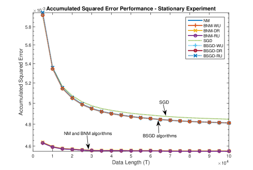
In this experiment, we consider the case where the desired data is generated by a stationary linear model. The input vectors $\mbox{$\mbox{\boldmath${x}$}$}_{t}=[x_{1}\ x_{2}\ 1]$ are 3-dimensional, where $[x_{1}\ x_{2}]$ is drawn from a jointly Gaussian random process and then scaled such that $\mbox{$\mbox{\boldmath${x}$}$}_{t}=[x_{1}\ x_{2}]^{T}\in[0\ 1]^{2}$. We include 1 as the third entry of $\mbox{$\mbox{\boldmath${x}$}$}_{t}$ to consider affine learners. Specifically the desired data is generated by $d_{t}=[1\ 1\ 1]^{T}\ \mbox{$\mbox{\boldmath${x}$}$}_{t}+\nu_{t}$, where $\nu_{t}$ is a random Gaussian noise with a variance of $0.01$.

In our simulations, we use $m=20$ WLs and $\mu=0.1$ for all SGD learners. In addition, for NM-based boosting algorithms, we set the forgetting factor $\beta=0.9999$ for all algorithms. Moreover, we choose $\sigma_{m}^{2}=0.02$ for SGD-based algorithms and $\sigma_{m}^{2}=0.004$ for NM-based algorithms, $K=5$ for data reuse approaches, and $c=1$ for all boosting algorithms. To achieve robustness, we average the results over 100 trials.

As depicted in Fig. 2, our proposed methods boost the performance of a single linear SGD-based WL. Nevertheless, we cannot further improve the performance of a linear NM-based WL in such a stationary experiment since the NM achieves the lowest MSE. We point out that the random updates method achieves the performance of the weighted updates method and the data reuse method with a much lower complexity. In addition, we observe that by increasing the data length, the performance improvement increases (Note that the distance between the ASE curves is slightly increasing).

Figure 2: The ASE performnce of the proposed algorithms in the stationary data experiment.

8.2 Chaotic Data

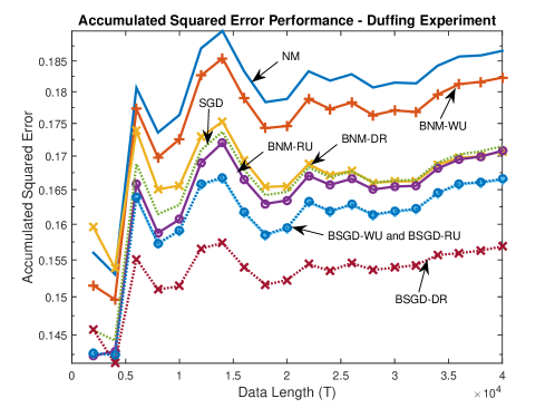
Here, in order to show the tracking capability of our algorithms in nonstationary environments, we consider the case where the desired data is generated by the Duffing map (Wiggins (2003)) as a chaotic model. Specifically, the data is generated by the following equation $x_{t+1}=2.75x_{t}-x_{t}^{3}-0.2x_{t-1}$, where we set $x_{-1}=0.9279$ and $x_{0}=0.1727$. We consider $d_{t}=x_{t+1}$ as the desired data and $[x_{t-1}\ x_{t}\ 1]$ as the input vector. In this experiment, each boosting algorithm uses 20 WLs. The step sizes for the SGD-based algorithms are set to $0.1$, the forgetting factor $\beta$ for the NM-based algorithms are set to $0.999$, and the modified desired MSE parameter $\sigma_{m}^{2}$ is set to $0.25$ for BSGD methods, and $0.17$ for the BNM methods. Note that although the value of $\sigma_{m}^{2}$ is higher than the achieved MSE, it can improve the performance significantly. This is because of the boosting effect, i.e., emphasizing on the harder data patterns. The figures show the superior performance of our algorithms over a single WL (whose step size is chosen to be the best), in this highly nonstationary environment. Moreover, as shown in Fig. 3, in the SGD-based boosted algorithms, the data reuse method shows a better performance relative to the other boosting methods. However, the random updates method has a significantly lower time consumption, which makes it desirable for larger data lengths. From the Fig. 3, one can see that our method is truly boosting the performance of the conventional linear WLs in this chaotic environment.

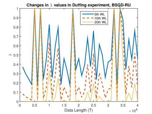
From the Fig. 4, we observe the approximate changes of the weights, in the BSGD-RU algorithm running over the Duffing data. As shown in this figure, the weights do not change monotonically, and this shows the capability of our algorithm in effective tracking of the nonstationary data. Furthermore, since we update the WLs in an ordered manner, i.e., we update the $(k+1)^{th}$ WL after the $k^{th}$ WL is updated, the weights assigned to the last WLs are generally smaller than the weights assigned to the previous WLs. As an example, in Fig. 4 we see that the weights assigned to the $5^{th}$ WL are larger than those of the $10^{th}$ and $20^{th}$ WLs. Furthermore, note that in this experiment, the dependency parameter $c$ is set to 1. We should mention that increasing the value of this parameter, in general, causes the lower weights, hence, it can considerably reduce the complexity of the random updates and data reuse methods.

Figure 3: ASE performance of the proposed methods on a Duffing data set.

Figure 4: The changing of the weights in BSGD-RU algorithm in the Duffing data experiment.

8.3 The Effect of Parameters

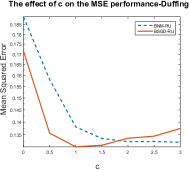
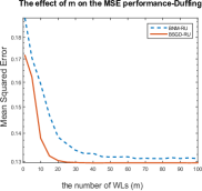
In this section, we investigate the effects of the dependence parameter $c$ and the modified desired MSE $\sigma_{m}^{2}$ as well as the number of WLs ,$m$, on the boosting performance of our methods in the Duffing data experiment, explained in Section 8.2. From the results in Fig. 5(c), we observe that, increasing the number of WLs up to $30$ can improve the performance significantly, while further increasing of $m$ only increases the computational complexity without improving the performance. In addition, as shown in Fig. 5(b), in this experiment, the dependency parameter $c$ has an optimum value around $1$. We note that choosing small values for $c$ reduces the boosting effect, and causes the weights to be larger, which in turn increases the computational complexity in random updates and data reuse approaches. On the other hand, choosing very large values for $c$ increases the dependency, i.e., in this case the generated weights are very close to $1$ or $0$, hence, the boosting effect is decreased. Overall, one should choose values around $1$ for $c$ to avoid those extreme cases.

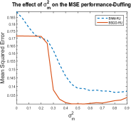
Furthermore, as depicted in Fig. 5(a), there is an optimum value around $0.5$ for $\sigma_{m}^{2}$ in this experiment. Note that, choosing small values for $\sigma_{m}^{2}$ results in large weights, thus, increases the complexity and reduces the diversity. However, choosing higher values for $\sigma_{m}^{2}$ results in smaller weights, and in turn reduces the complexity. Nevertheless, we note that increasing the value of $\sigma_{m}^{2}$ does not necessarily enhance the performance. Through the experiments, we find out that $\sigma_{m}^{2}$ must be in the order of the MSE amount to obtain the best performance.

(a) The effect of the parameter $\sigma_{m}^{2}$

(b) The effect of the parameter $c$

(c) The effect of the parameter $m$

Figure 5: The effect of the parameters $\sigma_{m}^{2}$, $c$, and $m$, on the MSE performance of the BNM-RU and BSGD-RU algorithms in the Duffing data experiment.

8.4 Benchmark Real and Synthetic Data Sets

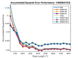
In this section, we demonstrate the efficiency of the introduced methods over some widely used real life machine learning regression data sets. We have normalized each dimension of the data to the interval $[-1,1]$ in all algorithms. We present the MSE performance of the algorithms in Table 1. These experiments show that our algorithms can successfully improve the performance of single linear WLs. We now describe the experiments and provide the results:

	SGD	BSGD-WU	BSGD-DR	BSGD-RU	NM	BNM-WU	BNM-DR	BNM-RU
MV	0.2711	0.2707	0.2706	0.2707	0.2592	0.2645	0.2587	0.2584
Puma8NH	0.1340	0.1334	0.1332	0.1334	0.1296	0.1269	0.1295	0.1284
Kinematics	0.0835	0.0831	0.0830	0.0831	0.0804	0.0801	0.0803	0.0801
Compactiv	0.0606	0.0599	0.0608	0.0598	0.0137	0.0086	0.0304	0.0078
Protein Tertiary	0.2554	0.2550	0.2549	0.2550	0.2370	0.2334	0.2385	0.2373
ONP	0.0015	0.0009	0.0009	0.0009	0.0009	0.0009	0.0009	0.0009
California Housing	0.0446	0.0450	0.0452	0.0448	0.0685	0.0671	0.0579	0.0683
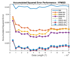
YPMSD	0.0237	0.0237	0.0233	0.0237	0.0454	0.0337	0.0302	0.0292

Table 1: The MSE of the proposed algorithms on real data sets.

Here, we briefly explain the details of the data sets:

1. MV: This is an artificial dataset with dependencies between the attribute values. One can refer to (Torgo ) for further details. There are $10$ attributes and one target value. In this dataset, we can slightly improve the performance of a single linear WL by using any of the proposed methods.

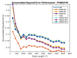
2. Puma Dynamics (Puma8NH): This dataset is a realistic simulation of the dynamics of a Puma $560$ robot arm (Torgo ). The task is to predict the angular acceleration of one of the robot arm’s links. The inputs include angular positions, velocities and torques of the robot arm. According to the ASE results in Fig. 6(a), the BNM-WU has the best boosting performance in this experiment. Nonetheless, the SGD-based methods also improve the performance.

3. Kinematics: This dataset is concerned with the forward kinematics of an 8 link robot arm (Torgo ). We use the variant 8nm, which is highly non-linear and noisy. As shown in Fig. 6(b), our proposed algorithms slightly improve the performance in this experiment.

4. Computer Activity (Compactiv): This real dataset is a collection of computer systems activity measures (Torgo ). The task is to predict USR, the portion of time that CPUs run in user mode from all attributes (Torgo ). The NM-based boosting algorithms deliver a significant performance improvement in this experiment, as shown by the results in Table 1.

5. Protein Tertiary (Lichman (2013)): This dataset is collected from Critical Assessment of protein Structure Prediction (CASP) experiments $5-9$. The aim is to predict the size of the residue using $9$ attributes over $45730$ data instances.

6. Online News Popularity (ONP) (Lichman (2013); Pereira et al. (2015)): This dataset summarizes a heterogeneous set of features about articles published by Mashable in a period of two years. The goal is to predict the number of shares in social networks (popularity).

7. California Housing: This dataset has been obtained from StatLib repository. They have collected information on the variables using all the block groups in California from the 1990 Census. Here, we seek to find the house median values, based on the given attributes. For further description one can refer to (Torgo ).

8. Year Prediction Million Song Dataset (YPMSD) (Bertin-Mahieux et al. (2011)): The aim is predicting the release year of a song from its audio features. Songs are mostly western, commercial tracks ranging from 1922 to 2011, with a peak in the year 2000s. We use a subset of the Million Song Dataset (Bertin-Mahieux et al. (2011)). As shown in Table 1 and Fig. 6(c), our algorithms can significantly improve the performance of the linear WL in this experiment.

(a) Puma8NH

(b) Kinematics.

(c) YPMSD

Figure 6: The performance of the proposed boosting methods on three real life data sets.

9 Conclusion

We introduced a novel family of boosted online regression algorithms and proposed three different boosting approaches, i.e., weighted updates, data reuse, and random updates, which can be applied to different online learning algorithms. We provide theoretical bounds for the MSE performance of our proposed methods in a strong mathematical sense. We emphasize that while using the proposed techniques, we do not assume any prior information about the statistics of the desired data or feature vectors. We show that by the proposed boosting approaches, we can significantly improve the MSE performance of the conventional SGD and NM algorithms. Moreover, we provide an upper bound for the weights generated during the algorithm that leads us to a thorough analysis of the computational complexity of these methods. The computational complexity of the random updates method is remarkably lower than that of the conventional mixture-of-experts and other variants of the proposed boosting approaches, without degrading the performance. Therefore, the boosting using random updates approach is an elegant alternative to the conventional mixture-of-experts method when dealing with real life large scale problems. We provide several results that demonstrate the strength of the proposed algorithms over a wide variety of synthetic as well as real data.

Appendices

Appendix A Proof of Lemma 1.

We observe that according to Algorithm 1,

$$l_{t}^{(M+1)} =\sum_{k=1}^{M}[\sigma_{m}^{2}-(e_{t}^{(k)})^{2}],$$

$$e_{t} =\frac{1}{M}\sum_{k=1}^{M}e_{t}^{(k)},$$

In addition, we have

$$\sum_{k=1}^{M}\left(e_{t}^{(k)}\right)^{2}\geq\frac{1}{M}\left(\sum_{k=1}^{M}e_{t}^{(k)}\right)^{2},$$

and as a result, if $e_{t}^{2}>\sigma_{m}^{2}$, then $l_{t}^{(M+1)}\leq 0$, i.e., $\lambda_{t}^{(M+1)}=1$. Hence by defining a modified desired MSE as $\sigma_{m}^{2}\triangleq\frac{\sigma_{d}^{2}-\kappa}{1-\kappa}$, and $\mbox{\boldmath${z}$}_{t}=[1/M,...,1/M]$ for $t=1,...,T$, we have

$$\frac{|\{t:e_{t}^{2}>\sigma_{m}^{2}\}|}{T} =\frac{|\{t:\lambda_{t}^{(M+1)}=1\}|}{T}$$

$$\leq\frac{\sum_{t=1}^{T}\lambda_{t}^{(M+1)}}{T}$$

$$\leq\kappa.$$

Finally we have

$$\frac{\sum_{t=1}^{T}e_{t}^{2}}{T} =\frac{\sum_{t;e_{t}^{2}\leq\sigma_{m}^{2}}e_{t}^{2}}{T}+\frac{\sum_{t;e_{t}^{2}>\sigma_{m}^{2}}e_{t}^{2}}{T}$$

$$\leq\frac{\sum_{t;e_{t}^{2}\leq\sigma_{m}^{2}}\sigma_{m}^{2}}{T}+\frac{\sum_{t;e_{t}^{2}>\sigma_{m}^{2}}1}{T}$$

$$\leq(1-\kappa)\sigma_{m}^{2}+\kappa$$

$$=\sigma_{d}^{2}.$$

This completes the proof of Lemma 1. $\Box$

Appendix B Proof of Lemma 2.

We have

$$\sum_{t=1}^{T}\sum_{k=1}^{M}\lambda_{t}^{(k)}\left[1-\left(e_{t}^{(k)}\right)^{2}\right]\geq(1-4\sigma^{2})\sum_{t=1}^{T}\sum_{k=1}^{M}\lambda_{t}^{(k)}.$$

Moreover, since $0\geq-\left(e_{t}^{(k)}\right)^{2}=l_{t}^{(k+1)}-l_{t}^{(k)}-\sigma_{m}^{2}\geq-4$, following the similar lines as the proof of Lemma 5 in (Servedio (2003)), we find that

$$\sum_{t=1}^{T}\sum_{k=1}^{M}\lambda_{t}^{(k)}\left[1-\left(e_{t}^{(k)}\right)^{2}\right]\leq-\sigma^{4}\sigma_{m}^{2}\sum_{t=1}^{T}\sum_{k=1}^{M}\lambda_{t}^{(k)}+\frac{1}{\sigma\ln(1/\sigma)}.$$

Since $\sum_{t=1}^{T}\sum_{k=1}^{M}\lambda_{t}^{(k)}\geq\kappa TM$, we conclude that

$$M\leq\frac{1}{(\kappa\sigma\ln(1/\sigma))(1-4\sigma^{2}+\sigma^{4}\sigma_{m}^{2})}.$$

This concludes the proof of Lemma 2. $\Box$

References

- Arenas-Garcia et al. (2016) Arenas-Garcia, J., Azpicueta-Ruiz, L. A., Silva, M. T. M., Nascimento, V. H., and Sayed, A. H. Combinations of adaptive filters: Performance and convergence properties. IEEE Signal Processing Magazine, 33(1):120–140, Jan 2016. ISSN 1053-5888. doi: 10.1109/MSP.2015.2481746.
- Azoury and Warmuth (2001) Azoury, K. S. and Warmuth, M. K. Relative loss bounds for on-line density estimation with the exponential family of distributions. Machine Learning, 43:211–246, 2001.
- Babenko et al. (2009) Babenko, B., Yang, M. H., and Belongie, S. A family of online boosting algorithms. In Computer Vision Workshops (ICCV Workshops), 2009 IEEE 12th International Conference on, pages 1346–1353, Sept 2009. doi: 10.1109/ICCVW.2009.5457453.
- Bauer and Kohavi (1999) Bauer, E. and Kohavi, R. An empirical comparison of voting classification algorithms: Bagging, boosting, and variants. Machine Learning, 36(1):105–139, 1999. ISSN 1573-0565. doi: 10.1023/A:1007515423169. URL http://dx.doi.org/10.1023/A:1007515423169.
- Ben-David et al. (1997) Ben-David, S., Kushilevitz, E., and Mansour, Y. Online learning versus offline learning. Machine Learning, 29(1):45–63, 1997. ISSN 1573-0565. doi: 10.1023/A:1007465907571. URL http://dx.doi.org/10.1023/A:1007465907571.
- Bertin-Mahieux et al. (2011) Bertin-Mahieux, T., Ellis, D. P., Whitman, B., and Lamere, P. The million song dataset. In Proceedings of the 12th International Conference on Music Information Retrieval (ISMIR 2011), 2011.
- Bertoni et al. (1997) Bertoni, A., Campadelli, P., and Parodi, M. A boosting algorithm for regression. volume 1327, pages 343–348. Springer, 1997.
- Beygelzimer et al. (2015a) Beygelzimer, A., Hazan, E., Kale, S., and Luo, H. Online gradient boosting. CoRR, abs/1506.04820, 2015a.
- Beygelzimer et al. (2015b) Beygelzimer, A., Kale, S., and Luo, H. Optimal and adaptive algorithms for online boosting. CoRR, abs/1502.02651, 2015b.
- Bottou and Bousquet (2008) Bottou, L. and Bousquet, O. The tradeoffs of large scale learning. In NIPS, 2008.
- Breiman (1997) Breiman, L. Prediction games and arcing algorithms, 1997.
- Cesa-Bianchi and Lugosi (2006) Cesa-Bianchi, N. and Lugosi, G. Prediction, Learning, and Games. Cambridge University Press, 2006.
- Chapelle et al. (2011) Chapelle, O., Shivaswamy, P., Vadrevu, S., Weinberger, K., Zhang, Y., and Tseng, B. Boosted multi-task learning. Machine Learning, 85(1):149–173, 2011. ISSN 1573-0565. doi: 10.1007/s10994-010-5231-6. URL http://dx.doi.org/10.1007/s10994-010-5231-6.
- Chen et al. (2012) Chen, S.-T., Lin, H.-T., and Lu, C.-J. An online boosting algorithm with theoretical justifications. In ICML, 2012.
- Demiriz et al. (2002) Demiriz, A., Bennett, K. P., and Shawe-Taylor, J. Linear programming boosting via column generation. Machine Learning, 46(1):225–254, 2002. ISSN 1573-0565. doi: 10.1023/A:1012470815092. URL http://dx.doi.org/10.1023/A:1012470815092.
- Dietterich (2000) Dietterich, T. G. An experimental comparison of three methods for constructing ensembles of decision trees: Bagging, boosting, and randomization. Machine Learning, 40(2):139–157, 2000. ISSN 1573-0565. doi: 10.1023/A:1007607513941. URL http://dx.doi.org/10.1023/A:1007607513941.
- Duda et al. (2001) Duda, R. O., Hart, P. E., and Stork, D. G. Pattern Classification. John Willey and Sons, 2001.
- Duffy and Helmbold (2002) Duffy, N. and Helmbold, D. Boosting methods for regression. Machine Learning, 47(2):153–200, 2002. ISSN 1573-0565. doi: 10.1023/A:1013685603443. URL http://dx.doi.org/10.1023/A:1013685603443.
- Fern and Givan (2003) Fern, A. and Givan, R. Online ensemble learning: An empirical study. Machine Learning, 53(1):71–109, 2003. ISSN 1573-0565. doi: 10.1023/A:1025619426553. URL http://dx.doi.org/10.1023/A:1025619426553.
- Freund and E.Schapire (1997) Freund, Y. and E.Schapire, R. A decision-theoretic generalization of on-line learning and an application to boosting. Journal of Computer and System Sciences, 55:119–139, 1997.
- Freund (1995) Freund, Y. Boosting a weak learning algorithm by majority. Inf. Comput., 121(2):256–285, September 1995. ISSN 0890-5401. doi: 10.1006/inco.1995.1136.
- Freund (2001) Freund, Y. An adaptive version of the boost by majority algorithm. Machine Learning, 43(3):293–318, 2001. ISSN 1573-0565. doi: 10.1023/A:1010852229904. URL http://dx.doi.org/10.1023/A:1010852229904.
- Jin and Zhang (2007) Jin, R. and Zhang, J. Multi-class learning by smoothed boosting. Machine Learning, 67(3):207–227, 2007. ISSN 1573-0565. doi: 10.1007/s10994-007-5005-y. URL http://dx.doi.org/10.1007/s10994-007-5005-y.
- Khan et al. (2016) Khan, F., Kari, D., Karatepe, I. A., and Kozat, S. S. Universal nonlinear regression on high dimensional data using adaptive hierarchical trees. IEEE Transactions on Big Data, 2(2):175–188, June 2016. doi: 10.1109/TBDATA.2016.2555323.
- Kozat and Singer (Jan. 2008) Kozat, S. S. and Singer, A. C. Universal switching linear least squares prediction. IEEE Transactions on Signal Processing, 56:189–204, Jan. 2008.
- Kozat et al. (2007) Kozat, S. S., Singer, A. C., and Zeitler, G. C. Universal piecewise linear prediction via context trees. IEEE Transactions on Signal Processing, 55(7):3730–3745, July 2007. ISSN 1053-587X. doi: 10.1109/TSP.2007.894235.
- Kozat et al. (2010) Kozat, S. S., Erdogan, A. T., Singer, A. C., and Sayed, A. H. Steady state MSE performance analysis of mixture approaches to adaptive filtering. IEEE Transactions on Signal Processing, 2010.
- Lichman (2013) Lichman, M. UCI machine learning repository, 2013. URL http://archive.ics.uci.edu/ml.
- Lu et al. (2016) Lu, J., Zhao, P., and Hoi, S. C. H. Online passive-aggressive active learning. Machine Learning, 103(2):141–183, 2016. ISSN 1573-0565. doi: 10.1007/s10994-016-5555-y. URL http://dx.doi.org/10.1007/s10994-016-5555-y.
- Malik (2013) Malik, P. Governing big data: Principles and practices. IBM J. Res. Dev., 57(3-4):1:1–1:1, May 2013. ISSN 0018-8646. doi: 10.1147/JRD.2013.2241359.
- Mannor and Meir (2002) Mannor, S. and Meir, R. On the existence of linear weak learners and applications to boosting. Machine Learning, 48(1):219–251, 2002. ISSN 1573-0565. doi: 10.1023/A:1013959922467. URL http://dx.doi.org/10.1023/A:1013959922467.
- Merhav and Feder (1993) Merhav, N. and Feder, M. Universal schemes for sequential decision from individual data sequences. IEEE Trans. Inform. Theory, 39:1280–1291, 1993.
- Oza and Russell (2001) Oza, N. C. and Russell, S. Online bagging and boosting. In Proceedings of AISTATS, 2001.
- Papoulis and Pillai (2002) Papoulis, A. and Pillai, S. U. Probability, Random Variables, and Stochastic Processes. McGraw-Hill Higher Education, 4 edition, 2002. ISBN 978-0-07-366011-0.
- Pereira et al. (2015) Pereira, F., Machado, P., Costa, E., and Cardoso, A. Progress in Artificial Intelligence: 17th Portuguese Conference on Artificial Intelligence, EPIA 2015, Coimbra, Portugal. Lecture Notes in Computer Science. Springer International Publishing, 2015. ISBN 9783319234854.
- Saigo et al. (2009) Saigo, H., Nowozin, S., Kadowaki, T., Kudo, T., and Tsuda, K. gboost: a mathematical programming approach to graph classification and regression. Machine Learning, 75(1):69–89, 2009. ISSN 1573-0565. doi: 10.1007/s10994-008-5089-z. URL http://dx.doi.org/10.1007/s10994-008-5089-z.
- Sayed (2003) Sayed, A. H. Fundamentals of Adaptive Filtering. John Wiley and Sons, 2003.
- Schapire and Freund (2012) Schapire, R. E. and Freund, Y. Boosting: Foundations and Algorithms. MIT Press, 2012.
- Schapire and Singer (1999) Schapire, R. E. and Singer, Y. Improved boosting algorithms using confidence-rated predictions. Machine Learning, 37(3):297–336, 1999. ISSN 1573-0565. doi: 10.1023/A:1007614523901. URL http://dx.doi.org/10.1023/A:1007614523901.
- Servedio (2003) Servedio, R. A. Smooth boosting and learning with malicious noise. Journal of Machine Learning Research, 4:633–648, 2003.
- Shaffer and Williams (1983) Shaffer, S. and Williams, C. S. Comparison of lms, alpha-lms, and data reusing lms algorithms. In Conference Record of the Seventeenth Asilomar Conference on Circuits, Systems and Computers, 1983.
- Shalev-Shwartz (2012) Shalev-Shwartz, S. Online learning and online convex optimization. Foundations and Trends in Machine Learning, 4:107–194, 2012.
- Shalev-Shwartz and Singer (2010) Shalev-Shwartz, S. and Singer, Y. On the equivalence of weak learnability and linear separability: new relaxations and efficient boosting algorithms. Machine Learning, 80(2):141–163, 2010. ISSN 1573-0565. doi: 10.1007/s10994-010-5173-z. URL http://dx.doi.org/10.1007/s10994-010-5173-z.
- Shrestha and Solomatine (2006) Shrestha, D. L. and Solomatine, D. P. Experiments with adaboost.rt, an improved boosting scheme for regression. In Experiments with AdaBoost.RT, an improved boosting scheme for regression, 2006.
- Singer et al. (2002) Singer, A. C., Kozat, S. S., and Feder, M. Universal linear least squares prediction:upper and lower bounds. IEEE Transactions on Information Theory, 48(8):2354–2362, 2002.
- Soltanmohammadi et al. (2016) Soltanmohammadi, E., Naraghi-Pour, M., and van der Schaar, M. Context-based unsupervised ensemble learning and feature ranking. Machine Learning, 105(3):459–485, 2016. ISSN 1573-0565. doi: 10.1007/s10994-016-5576-6. URL http://dx.doi.org/10.1007/s10994-016-5576-6.
- Taieb and Hyndman (2013) Taieb, B. and Hyndman, R. J. A gradient boosting approach to the kaggle load forecasting competition. International Journal of Forecasting, pages 1–19, 2013.
- Taieb and Hyndman (2014) Taieb, B. and Hyndman, R. J. Boosting multi-step autoregressive forecasts. In ICML, 2014.
- (49) Torgo, L. Regression data sets. URL http://www.dcc.fc.up.pt/ltorgo/Regression/DataSets.html.
- Vanli and Kozat (2014) Vanli, N. D. and Kozat, S. S. A comprehensive approach to universal piecewise nonlinear regression based on trees. IEEE Transactions on Signal Processing, 62(20):5471–5486, Oct 2014.
- Wiggins (2003) Wiggins, S. Introduction to Applied Nonlinear Dynamical Systems and Chaos. Springer New York, 2003. ISBN 9780387001777.