Approximate Message Passing with Nearest Neighbor Sparsity Pattern Learning

Abstract

We consider the problem of recovering clustered sparse signals with no prior knowledge of the sparsity pattern. Beyond simple sparsity, signals of interest often exhibits an underlying sparsity pattern which, if leveraged, can improve the reconstruction performance. However, the sparsity pattern is usually unknown a priori. Inspired by the idea of k-nearest neighbor (k-NN) algorithm, we propose an efficient algorithm termed approximate message passing with nearest neighbor sparsity pattern learning (AMP-NNSPL), which learns the sparsity pattern adaptively. AMP-NNSPL specifies a flexible spike and slab prior on the unknown signal and, after each AMP iteration, sets the sparse ratios as the average of the nearest neighbor estimates via expectation maximization (EM). Experimental results on both synthetic and real data demonstrate the superiority of our proposed algorithm both in terms of reconstruction performance and computational complexity.

I Introduction

Compressed sensing (CS) aims to accurately reconstruct sparse signals from undersampled linear measurements[1, 2, 3]. To this end, a plethora of methods have been studied in the past years. Among others, approximate message passing (AMP) [4] proposed by Donoho et al. is one state-of-the-art algorithm to address sparse signal reconstruction in CS. Moreover, AMP has been extended to Bayesian AMP (B-AMP) [5, 6] and general linear mixing problems[7, 8, 9]. While many practical signals can be described as sparse, they often exhibit an underlying structure, e.g., the nonzero coefficients occur in clusters[10, 11, 12, 13, 14, 15, 16]. Exploiting such intrinsic structure beyond simple sparsity can significantly boost the reconstruction performance[14, 15, 16]. To this end, various algorithms have been proposed, e.g., group LASSO[10], StructOMP[17], Graph-CoSaMP[18], and block sparse Bayesian learning (B-SBL)[19, 20, 21], etc. However, these algorithms require knowledge of sparsity pattern which is usually unknown a priori. To reconstruct sparse signals with unknown structure, a number of methods[22, 23, 24, 25, 26, 27, 28] have been developed to use various structured priors to encourage both sparsity and cluster patterns simultaneously. The main effort of these algorithms lies in constructing a hierarchical prior model, e.g., Markov tree[23], structured spike and slab[24, 25], hierarchical Gamma-Gaussian[26, 27, 28] to encode the structured sparsity pattern.

In this letter, we take an alternative approach and propose an efficient message passing algorithm, termed AMP with nearest neighbor sparsity pattern learning (AMP-NNSPL), to recover clustered sparse signals adaptively, i.e., without any prior knowledge of the sparsity pattern. For clustered sparse signals, if the nearest neighbors of one element are zeros (nonzeros), it will tend to be zero (nonzero) with high probability, a similar idea of k-nearest neighbor (k-NN) algorithm which assumes that data close together more likely belong to the same category[29, 30]. Therefore, instead of explicitly modeling the sophisticated sparsity pattern, AMP-NNSPL specifies a flexible spike and slab prior on the unknown signal and, after each AMP iteration, updates the sparse ratios as the average of their nearest neighbor estimates via expectation maximization (EM)[31]. In this way, the sparsity pattern is learned adaptively. Simulations results on both synthetic and real data demonstrate the superiority of our proposed algorithm both in terms of reconstruction performance and computational efficiency.

II System Model

Consider the following linear Gaussian model

$$\mathbf{y}=\mathbf{Ax}+\mathbf{w},$$ (1)

where $\mathbf{x}\in\mathbb{R}^{N}$ is the unknown signal, $\mathbf{y}\in\mathbb{R}^{M}$ is the available measurements, $\mathbf{A}\in\mathbb{R}^{M\times N}$ is the known measurement matrix, and $\mathbf{w}\in\mathbb{R}^{M}\sim\mathcal{N}\bigl{(}\mathbf{w};0,\Delta_{0}\mathbf{I}\bigr{)}$ is the additive noise. $\mathcal{N}\bigl{(}\mathbf{x};\mathbf{m},\mathbf{C}\bigr{)}$ denotes a Gaussian distribution of $\mathbf{x}$ with mean $\mathbf{m}$ and covariance $\mathbf{C}$ and $\mathbf{I}$ denotes the identity matrix. Our goal is to estimate $\mathbf{x}$ from $\mathbf{y}$ when $M\ll N$ and $\mathbf{x}$ is clustered sparse while its specific sparsity pattern is unknown a priori.

To enforce sparsity, from a Bayesian perspective, the signals are assumed to follow sparsity-promoting prior distributions, e.g., Laplace prior[32], automatic relevance determination [33], and spike and slab prior[34, 6]. In this letter we consider a flexible spike and slab prior of the form

$$p_{0}(\mathbf{x})=\stackrel{{\scriptstyle[}}{{i}}=1]{N}{\prod}p_{0}(x_{i})=\stackrel{{\scriptstyle[}}{{i}}=1]{N}{\prod}\bigl{[}\bigl{(}1-\lambda_{i}\bigr{)}\delta(x_{i})+\lambda_{i}f(x_{i})\bigr{]},$$ (2)

where $\lambda_{i}\in(0,1)$ is the sparse ratio, i.e., the probability of $x_{i}$ being nonzero, $\delta(x_{i})$ is the Dirac delta function, $f(x_{i})$ is the distribution of the nonzero entries in $\mathbf{x}$, e.g., $f(x_{i})=\mathcal{N}(x_{i};\mu_{0},\tau_{0})$ for sparse Gaussian signals and $f(x_{i})=\delta(x_{i}-1)$ for sparse binary signals, etc.

It is important to note that in (2) we specify an individual $\lambda_{i}$ for each entry, as opposed to a common value in [34, 6]. This is a key feature that will be exploited by the proposed algorithm for reconstruction of structured sparse signals. Up to now, it seems that no structure is ever introduced to enforce the underlying sparsity pattern. Indeed, if the sparse ratios $\lambda_{i},i=1,\ldots,N$ are learned independently, we will not benefit from the potential structure. The main contribution of this letter is a novel adaptive learning method which encourages clustered sparsity, as descried in Section III.

III Proposed Algorithm

In this section, inspired by the idea of k-NN, we propose an adaptive reconstruction algorithm to recover clustered sparse signals without any prior knowledge of the sparsity pattern, e.g., structure and sparse ratio.

Before proceeding, we first give a brief description of AMP. Generally, AMP decouples the vector estimation problem (1) into $N$ scalar problems in the asymptotic regime[35, 36]

$$\mathbf{y}=\mathbf{Ax}+\mathbf{w}\longrightarrow\begin{cases}R_{1}=x_{1}+\tilde{w}_{1}\\ \vdots&,\\ R_{N}=x_{N}+\tilde{w}_{N}\end{cases}$$ (3)

where the effective noise $\tilde{w}_{i}$ asymptotically follows $\mathcal{N}\bigl{(}\tilde{w}_{i};0,\Sigma_{i}\bigr{)}$. The values of $R_{i},\Sigma_{i}$ are updated iteratively in each AMP iteration (see Algorithm 1) and the posterior distribution of $x_{i}$ is estimated as

$$q\bigl{(}x_{i}|R_{i},\Sigma_{i}\bigr{)}=\frac{1}{Z(R_{i},\Sigma_{i})}p_{0}\bigl{(}x_{i}\bigr{)}\mathcal{N}\bigl{(}x_{i};R_{i},\Sigma_{i}\bigr{)},$$ (4)

where $Z(R_{i},\Sigma_{i})$ is the normalization constant. From (4), the estimates of the mean and variance of $x_{i}$ are

$$g_{a}(R_{i},\Sigma_{i}) =\int x_{i}q\bigl{(}x_{i}|R_{i},\Sigma_{i}\bigr{)}dx_{i},$$ (5)

$$g_{c}(R_{i},\Sigma_{i}) =\int x_{i}^{2}q\bigl{(}x_{i}|R_{i},\Sigma_{i}\bigr{)}dx_{i}-g_{a}^{2}(R_{i},\Sigma_{i}).$$ (6)

For more details of AMP and its extensions, the readers are referred to [4, 5, 35, 6]. Two problems arise in traditional AMP. First, it assumes full knowledge of the prior distribution and noise variance, which is an impractical assumption. Second, it does not account for the potential structure of sparsity. In the sequel, we resort to expectation maximization (EM) to learn the unknown hyperparameters. Further, to encourage structured sparsity, we develop a nearest neighbor sparsity pattern learning rule motivated by the idea of k-NN algorithm. For lack of space, we only consider the sparse Gaussian case, $f\bigl{(}x_{i}\bigr{)}=\mathcal{N}\bigl{(}x_{i};\mu_{0},\tau_{0}\bigr{)},$ while generalization to other settings is possible.

The hidden variables are chosen as the unknown signal vector $\mathbf{x}$ and the hyperparameters are denoted by $\boldsymbol{\theta}$. The specific definition of $\boldsymbol{\theta}$ depends on the choice of distribution $f\bigl{(}x\bigr{)}$ in (2). In the Gaussian case, $\boldsymbol{\theta}=\bigl{\{}\mu_{0},\tau_{0},\Delta_{0},\lambda_{i},i=1,\ldots,N\bigr{\}}$ while in the binary case, $\boldsymbol{\theta}=\bigl{\{}\Delta_{0},\lambda_{i},i=1,\ldots,N\bigr{\}}$. Denote by $\boldsymbol{\theta}^{t}$ the estimate of hyperparameters at the $t$th EM iteration, then EM alternates between the following two steps[31]

$$Q\bigl{(}\boldsymbol{\theta},\boldsymbol{\theta}^{t}\bigr{)} =\mathsf{E}\Bigl{\{}\ln p\bigl{(}\mathbf{\mathbf{x}},\mathbf{y}\bigr{)}|\mathbf{y};\boldsymbol{\theta}^{t}\Bigr{\}},$$ (7)

$$\boldsymbol{\theta}^{t+1} =\arg\underset{\boldsymbol{\theta}}{\max}Q\bigl{(}\boldsymbol{\theta},\boldsymbol{\theta}^{t}\bigr{)},$$ (8)

where $\mathsf{E}\bigl{\{}\cdot|\mathbf{y};\boldsymbol{\theta}^{t}\bigr{\}}$ denotes expectation conditioned on observations $\mathbf{y}$ with parameters $\boldsymbol{\theta}^{t}$, i.e., the expectation is with respect to the posterior distribution $p\bigl{(}\mathbf{\mathbf{x}}|\mathbf{y};\boldsymbol{\theta}^{t}\bigr{)}$. From (1), (2), the joint distribution $p(\mathbf{\mathbf{x}},\mathbf{y})$ in (7) is defined as

$$p(\mathbf{\mathbf{x}},\mathbf{y})=p\bigl{(}\mathbf{y}|\mathbf{\mathbf{x}}\bigr{)}\prod_{i}(1-\lambda_{i})\delta(x_{i})+\lambda_{i}f(x_{i}),$$ (9)

where $p(\mathbf{y}|\mathbf{\mathbf{x}})=\mathcal{N}\bigl{(}\mathbf{y};\mathbf{Ax},\Delta_{0}\mathbf{I}\bigr{)}$. AMP offers an efficient approximation of $p\bigl{(}\mathbf{\mathbf{x}}|\mathbf{y};\boldsymbol{\theta}^{t}\bigr{)}$, denoted as $q\bigl{(}\mathbf{\mathbf{x}}|\mathbf{y};\boldsymbol{\theta}^{t}\bigr{)}=\prod_{i}q\bigl{(}x_{i}|R_{i},\Sigma_{i}\bigr{)}$, whereby the E step (7) can be efficiently calculated. Since joint optimization of $\mathbf{\boldsymbol{\theta}}$ is difficult, we adopt the incremental EM update rule proposed in [37], i.e., we update one or partial elements at a time while holding the other parameters fixed.

After some algebra, the marginal posterior distribution of $x_{i}$ in (4) can be written as

$$q\bigl{(}x_{i}|R_{i},\Sigma_{i}\bigr{)}=\bigl{(}1-\pi_{i}\bigr{)}\delta\bigl{(}x_{i}\bigr{)}+\pi_{i}\mathcal{N}\bigl{(}x_{i};m_{i},V_{i}\bigr{)},$$ (10)

where

$$V_{i} =\frac{\tau_{0}\Sigma_{i}}{\Sigma_{i}+\tau_{0}},$$ (11)

$$m_{i} =\frac{\tau_{0}R_{i}+\Sigma_{i}\mu_{0}}{\Sigma_{i}+\tau_{0}},$$ (12)

$$\pi_{i} =\frac{\lambda_{i}}{\lambda_{i}+\bigl{(}1-\lambda_{i}\bigr{)}\exp\bigl{(}-\mathcal{L}\bigr{)}},$$ (13)

$$\mathcal{L} =\frac{1}{2}\ln\frac{\Sigma_{i}}{\Sigma_{i}+\tau_{0}}+\frac{R_{i}^{2}}{2\Sigma_{i}}-\frac{\bigl{(}R_{i}-\mu_{0}\bigr{)}^{2}}{2\bigl{(}\Sigma_{i}+\tau_{0}\bigr{)}}.$$ (14)

Note that for notational brevity, we have omitted the iteration index $t$. The mean and variance defined in (5) and (6) can now be explicitly calculated as

$$g_{a}\bigl{(}R_{i},\Sigma_{i}\bigr{)} =\pi_{i}m_{i},$$ (15)

$$g_{c}\bigl{(}R_{i},\Sigma_{i}\bigr{)} =\pi_{i}\bigl{(}m_{i}^{2}+V_{i}\bigr{)}-g_{a}^{2}\bigl{(}R_{i},\Sigma_{i}\bigr{)}.$$ (16)

To learn the sparse ratios $\lambda_{i},i=1,\ldots,N$, we need to maximize $Q\bigl{(}\boldsymbol{\theta},\boldsymbol{\theta}^{t}\bigr{)}$ with respect to $\lambda_{i}$. After some algebra, we obtain the standard EM update equation as $\lambda_{i}^{t+1}=\pi_{i}^{t}$, which, albeit simple, fails to capture the inherent structure in the sparsity pattern. To address this problem, a novel learning rule is proposed as follows

$$\lambda_{i}^{t+1}=\frac{1}{\bigl{|}\mathcal{N}\bigl{(}i\bigr{)}\bigr{|}}\underset{j\in\mathcal{N}(i)}{\sum}\pi_{j}^{t},$$ (17)

where $\mathcal{N}\bigl{(}i\bigr{)}$ denotes the set of nearest neighbor indexes of element $x_{i}$ in $\mathbf{x}$ (1) and $\bigl{|}\mathcal{N}\bigl{(}i\bigr{)}\bigr{|}$ denotes the cardinality of $\mathcal{N}\bigl{(}i\bigr{)}$. For one dimensional (1D) data , $\mathcal{N}\bigl{(}i\bigr{)}=\bigl{\{}i-1,i+1\bigr{\}}$ and $\bigl{|}\mathcal{N}\bigl{(}i\bigr{)}\bigr{|}=2$, while for two dimensional (2D) data, $\mathcal{N}\bigl{(}i\bigr{)}=\bigl{\{}(q,l-1),(q,l+1),(q-1,l),(q+1,l)\bigr{\}}$ and $\bigl{|}\mathcal{N}\bigl{(}i\bigr{)}\bigr{|}=4$, where $(q,l)$ indicates the coordinates of $x_{i}$ in the 2D space. Generalizations to other cases can be made.

Note that in (17), we have chosen the nearest neighbor of each element, excluding itself, as the neighboring set. The estimate of one sparse ratio is not determined by its own estimate, but rather the average of its nearest neighbor estimates. The insight for this choice is that, for clustered sparse signals, if the nearest neighbors of one element are zero (nonzero), it will be zero (nonzero) with high probability, a similar idea to k-NN. If the neighboring set is chosen as the whole elements, the proposed algorithm reduces to EM-BG-GAMP[34, 6].

The leaning of other hyperparameters follows the standard rule of EM algorithm. Maximizing $Q\bigl{(}\boldsymbol{\theta},\boldsymbol{\theta}^{t}\bigr{)}$ with respect to $\Delta_{0}$ and after some algebra, we obtain

$$\Delta_{0}^{t+1}=\frac{1}{M}\sum_{a}\Bigl{[}\frac{\bigl{(}y_{a}-Z_{a}^{t}\bigr{)}^{2}}{\bigl{(}1+V_{a}^{t}/\Delta_{0}^{t}\bigr{)}^{2}}+\frac{\Delta_{0}^{t}V_{a}^{t}}{\Delta_{0}^{t}+V_{a}^{t}}\Bigr{]},$$ (18)

where $Z_{a}^{t}$ and $V_{a}^{t}$ are obtained within the AMP iteration and are defined in Algorithm 1. Similarly, maximizing $Q\bigl{(}\boldsymbol{\theta},\boldsymbol{\theta}^{t}\bigr{)}$ with respect to $\mu_{0}$ and $\tau_{0}$ results in the update equations

$$\mu_{0}^{t+1} =\frac{\sum_{i}\pi_{i}^{t}m_{i}^{t}}{\sum_{i}\pi_{i}^{t}},$$ (19)

$$\tau_{0}^{t+1} =\frac{1}{\sum_{i}\pi_{i}^{t}}\underset{i}{\sum}\pi_{i}^{t}\bigl{[}\bigl{(}\mu_{0}^{t}-m_{i}^{t}\bigr{)}^{2}+V_{i}\bigr{]}.$$ (20)

Valid initialization of the unknown hyperparameters is essential since EM algorithm may converge to a local maximum or a saddle point of the likelihood function[31]. The sparse ratios $\lambda_{i}$ and noise variance $\Delta_{0}$ are initialized as $\lambda_{i}^{1}=0.5$ and $\Delta_{0}^{1}=\bigl{\|}\mathbf{y}\bigr{\|}_{2}^{2}/M\bigl{(}\textrm{SNR}^{0}+1\bigr{)}$, respectively, where $\textrm{SNR}^{0}$ is suggested to be 100 [34]. For the sparse Gaussian case, active mean $\mu_{0}$ and variance $\tau_{0}$ are initialized as $\mu_{0}^{1}=0$, and $\tau_{0}^{1}=\bigl{(}\bigl{\|}\mathbf{y}\bigr{\|}_{2}^{2}-M\Delta_{0}^{1}\bigr{)}/\lambda_{i}^{1}\bigl{\|}\mathbf{A}\bigr{\|}_{F}^{2}$, respectively, where$\bigl{\|}\mathbf{\cdot}\bigr{\|}_{2}$, $\bigl{\|}\mathbf{\cdot}\bigr{\|}_{F}$ are the $l_{2}$ norm and Frobenius norm, respectively.

The proposed approximate message passing with nearest neighbor sparsity pattern learning (AMP-NNSPL) is summarized in Algorithm 1. The complexity of AMP-NNSPL is dominated by matrix-vector multiplications in the original AMP and thus only scales as $\mathcal{O}(MN)$, i.e., the proposed algorithm is computationally efficient.

Algorithm 1 AMP-NNSPL Algorithm

Input: $\mathbf{y}$ $\mathbf{A}$.

Initialization: Set $t=1$ and $T_{max},\epsilon_{toc}$. Initialize $\mu_{0},\tau_{0},\Delta_{0}$ and $\lambda_{i},i=1,\ldots,N$ as in Section III. $\hat{x}_{i}^{1}=\int x_{i}p_{0}(x_{i})dx_{i},\nu_{i}^{1}=\int|x_{i}-\hat{x}_{i}^{1}|^{2}p_{0}(x_{i})dx_{i},i=1,\ldots,N$, $V_{a}^{0}=1,Z_{a}^{0}=y_{a},a=1,\ldots,M.$

1) Factor node update: For $a=1,\ldots,M$

$$V_{a}^{t} =\sum_{i}|A_{ai}|^{2}\nu_{i}^{t},$$

$$Z_{a}^{t} =\sum_{i}A_{ai}\hat{x}_{i}^{t}-\frac{V_{a}^{t}}{\Delta_{0}^{t}+V_{a}^{t-1}}\bigl{(}y_{a}-Z_{a}^{t-1}\bigr{)}.$$

2) Variable node update: For $i=1,\ldots,N$

$$\Sigma_{i}^{t} =\Bigl{[}\sum_{a}\frac{|A_{ai}|^{2}}{\Delta_{0}^{t}+V_{a}^{t}}\Bigr{]}^{-1},$$

$$R_{i}^{t} =\hat{x}_{i}^{t}+\Sigma_{i}^{t}\sum_{a}\frac{A_{ai}\bigl{(}y_{a}-Z_{a}^{t}\bigr{)}}{\Delta_{0}^{t}+V_{a}^{t}},$$

$$\hat{x}_{i}^{t+1} =g_{a}\left(R_{i}^{t},\Sigma_{i}^{t}\right),$$

$$\hat{\nu}_{i}^{t+1} =g_{c}\left(R_{i}^{t},\Sigma_{i}^{t}\right).$$

3) Update $\lambda_{i}^{t+1},i=1,\ldots N$, as (17);

4) Update $\mu_{0}^{t+1},\tau_{0}^{t+1},\Delta_{0}^{t+1}$ as (19), (20), and (18);

5) Set $t\leftarrow t+1$ and proceed to step 1) until $T_{max}$ iterations or $\bigl{\|}\mathbf{\hat{x}}^{t+1}-\mathbf{\hat{x}}^{t}\bigr{\|}_{2}<\epsilon_{toc}\bigl{\|}\hat{\mathbf{x}}^{t}\bigr{\|}_{2}$ .

IV Numerical Experiments

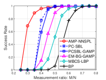
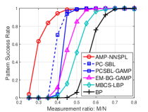
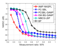
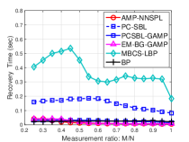
In this section, a series of numerical experiments are performed to demonstrate the performance of the proposed algorithm under various settings. Comparisons are made to some state-of-the-art methods which need no prior information of the sparstiy pattern, e.g., PC-SBL[26] and its AMP version PCSBL-GAMP[27], MBCS-LBP[28], and EM-BG-GAMP[34]. The performance of Basis Pursuit (BP) [38, 39, 40] is also evaluated. Throughout the experiments, we set the maximum number of iterations for AMP-NNSPL, PCSBL-GAMP, and EM-BG-GAMP to be $T_{max}=200$, and the tolerance value of termination to be $\epsilon_{toc}=10^{-6}.$ For other algorithms, we use the defaut setting. The elements of measurement matrix $\mathbf{A}\in\mathbb{R}^{M\times N}$ are independently generated following standard Gaussian distribution and the columns are normalized to unit norm. The success rate is defined as the ratio of the number of successful trials to the total number of experiments, where a trial is successful if the normalized mean square error (NMSE) is less than -60 dB, where $\mathsf{NMSE}=20\log_{10}(\bigl{\|}\mathbf{\hat{x}}-\mathbf{x}\bigr{\|}_{2}/\bigl{\|}\mathbf{x}\bigr{\|}_{2})$. The pattern recovery success rate is defined as the ratio of the number of successful trials to the total number of experiments, where a trial is successful if the support is exactly recovered. A coefficient whose magnitude is less than $10^{-4}$ is deemed as a zero coefficient.

IV-A Synthetic Data

We generate synthetic block-sparse signals in a similar way as [21, 26], where $K$ nonzero elements are partitioned into $L$ blocks with random sizes and random locations. Set $N=100,K=25,L=4$ and the nonzero elements are generated independently following Gaussian distribution with mean $\mu_{0}=3$ and variance $\tau_{0}=1$. The results are averaged over 1000 independent runs. Fig. 1 depicts the success rate and pattern recovery success rate. It can be seen that AMP-NNSPL achieves the highest success rate and pattern recovery rate at various measurement ratios. In the noisy setting, Fig. 2 shows the average NMSE and runtime of different algorithms when the signal to noise ratio (SNR) is 50 dB, where $SNR=20\log_{10}(\bigl{\|}\mathbf{A}\mathbf{x}\bigr{\|}_{2}/\bigl{\|}\mathbf{w}\bigr{\|}_{2})$. We see that AMP-NNSPL outperforms other methods both in terms of NMSE and computational efficiency.

Figure 1: Success rate (left) and pattern success rate (right) vs. $M/N$ for block-sparse signals $N=100$, $K=25$, $L=4$, noiseless case.

Figure 2: NMSE (left) and recovery time (right) vs. $M/N$ for block-sparse signals $N=100$, $K=25$, $L=4$, SNR = 50 dB.

IV-B Real Data

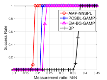
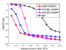
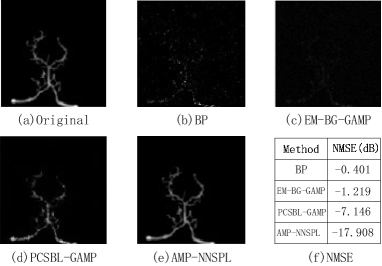
To evaluate the performance on real data, we consider a real angiogram image[18] of 100$\times$100 pixels with sparsity around 0.12. Fig. 3 depicts the success rate in noiseless case and NMSE at $SNR=50$ dB, respectively. The MBCS-LBP and PC-SBL algorithms are not included due to their high computational complexity. It can be seen that AMP-NNSPL significantly outperforms other methods both in terms of success rate and NMSE. In particular, when $M/N=0.12$ and $SNR=50$ dB, typical recovery results are illustrated in Fig. 4, which shows that AMP-NNSPL achives the best reconstruction performance.

Figure 3: Success rate (left) in noiseless case and NMSE (right) at $SNR=50\textrm{dB}$ vs. $M/N$ for real 2D angiogram image.

Figure 4: Recovery results of real 2D angiogram image in noisy setting when $M/N=0.12$ and $SNR=50$ dB.

V Conclusion

In this lettter, we propose an efficient algorithm termed AMP-NNSPL to recover clustered sparse signals when the sparsity pattern is unknown. Inspired by the k-NN algorithm, AMP-NNSPL learns the sparse ratios in each AMP iteration as the average of their nearest neighbor estimates using EM, thereby the sparsity pattern is learned adaptively. Experimental results on both synthetic and real data demonstrate the state-of-the-art performance of AMP-NNSPL.

References

- [1] D. L. Donoho, “Compressed sensing,” IEEE Trans. Inf. Theory, vol. 52, no. 4, pp. 1289–1306, Apr. 2006.
- [2] E. J. Candès and M. B. Wakin, “An introduction to compressive sampling,” IEEE Signal Process. Mag., vol. 25(2), pp. 21–30, Mar. 2008.
- [3] Y. C. Eldar and G. Kutyniok, Eds., Compressed sensing: theory and applications. Cambridge Univ. Press, 2012.
- [4] D. L. Donoho, A. Maleki, and A. Montanari, “Message-passing algorithms for compressed sensing,” in Proc. Nat. Acad. Sci., vol. 106, no. 45, Nov. 2009, pp. 18 914–18 919.
- [5] ——, “Message passing algorithms for compressed sensing: I. motivation and construction,” in IEEE Information Theory Workshop (ITW), Jan. 2010, pp. 1–5.
- [6] F. Krzakala, M. Mézard, F. Sausset, Y. Sun, and L. Zdeborová, “Probabilistic reconstruction in compressed sensing: algorithms, phase diagrams, and threshold achieving matrices,” Journal of Statistical Mechanics: Theory and Experiment, vol. 2012, no. 08, p. P08009, 2012.
- [7] S. Rangan, “Generalized approximate message passing for estimation with random linear mixing,” in Proc. IEEE Int. Symp. Inf. Theory, 2011, pp. 2168–2172.
- [8] P. Schniter, “A message-passing receiver for BICM-OFDM over unknown clustered-sparse channels,” IEEE J. Sel. Topics Signal Process., vol. 5, no. 8, pp. 1462–1474, Dec. 2011.
- [9] U. S. Kamilov, S. Rangan, A. K. Fletcher, and M. Unser, “Approximate message passing with consistent parameter estimation and applications to sparse learning,” IEEE Trans. Inf. Theory, vol. 60(5), pp. 2969–2985, May. 2014.
- [10] M. Yuan and Y. Lin, “Model selection and estimation in regression with grouped variables,” Journal of the Royal Statistical Society: Series B (Statistical Methodology), vol. 68, no. 1, pp. 49–67, 2006.
- [11] V. Cevher, P. Indyk, C. Hegde, and R. G. Baraniuk, “Recovery of clustered sparse signals from compressive measurements,” DTIC Document, Tech. Rep., 2009.
- [12] M. Stojnic, F. Parvaresh, and B. Hassibi, “On the reconstruction of block-sparse signals with an optimal number of measurements,” IEEE Trans. Signal Process., vol. 57, no. 8, pp. 3075–3085, 2009.
- [13] R. G. Baraniuk, V. Cevher, M. F. Duarte, and C. Hegde, “Model-based compressive sensing,” IEEE Trans. Inf. Theory, vol. 56, no. 4, pp. 1982–2001, 2010.
- [14] J. Huang, T. Zhang et al., “The benefit of group sparsity,” The Annals of Statistics, vol. 38, no. 4, pp. 1978–2004, 2010.
- [15] Y. C. Eldar and M. Mishali, “Robust recovery of signals from a structured union of subspaces,” IEEE Trans. Inf. Theory, vol. 55, no. 11, pp. 5302–5316, 2009.
- [16] Y. C. Eldar, P. Kuppinger, and H. Bölcskei, “Block-sparse signals: Uncertainty relations and efficient recovery,” IEEE Trans. Signal Process., vol. 58, no. 6, pp. 3042–3054, 2010.
- [17] J. Huang, T. Zhang, and D. Metaxas, “Learning with structured sparsity,” The Journal of Machine Learning Research, vol. 12, pp. 3371–3412, 2011.
- [18] C. Hegde, P. Indyk, and L. Schmidt, “A nearly-linear time framework for graph-structured sparsity,” in Proceedings of The 32nd International Conference on Machine Learning, 2015, pp. 928–937.
- [19] D. P. Wipf and B. D. Rao, “An empirical Bayesian strategy for solving the simultaneous sparse approximation problem,” IEEE Trans. Signal Process., vol. 55, no. 7, pp. 3704–3716, 2007.
- [20] Z. Zhang and B. D. Rao, “Sparse signal recovery with temporally correlated source vectors using sparse bayesian learning,” IEEE J. Sel. Topics Signal Process., vol. 5, no. 5, pp. 912–926, 2011.
- [21] Z. Zhang and B. Rao, “Extension of SBL algorithms for the recovery of block sparse signals with intra-block correlation,” IEEE Trans. on Signal Process., vol. 61, no. 8, pp. 2009–2015, 2013.
- [22] L. He and L. Carin, “Exploiting structure in wavelet-based bayesian compressive sensing,” IEEE Trans. Signal Process., vol. 57, no. 9, pp. 3488–3497, 2009.
- [23] S. Som and P. Schniter, “Compressive imaging using approximate message passing and a markov-tree prior,” IEEE Trans. Signal Process., vol. 60, no. 7, pp. 3439–3448, 2012.
- [24] L. Yu, H. Sun, J.-P. Barbot, and G. Zheng, “Bayesian compressive sensing for cluster structured sparse signals,” Signal Processing, vol. 92, no. 1, pp. 259–269, 2012.
- [25] M. R. Andersen, O. Winther, and L. K. Hansen, “Spatio-temporal spike and slab priors for multiple measurement vector problems,” arXiv preprint arXiv:1508.04556, 2015.
- [26] J. Fang, Y. Shen, H. Li, and P. Wang, “Pattern-coupled sparse Bayesian learning for recovery of block-sparse signals,” IEEE Trans. on Signal Process., vol. 63, no. 2, pp. 360–372, 2015.
- [27] J. Fang, L. Zhang, and H. Li, “Two-dimensional pattern-coupled sparse Bayesian learning via generalized approximate message passing,” arXiv preprint arXiv:1505.06270, 2015.
- [28] L. Yu, H. Sun, G. Zheng, and J. P. Barbot, “Model based Bayesian compressive sensing via local beta process,” Signal Processing, vol. 108, pp. 259–271, 2015.
- [29] E. Fix and J. L. Hodges Jr, “Discriminatory analysis-nonparametric discrimination: consistency properties,” DTIC Document, Tech. Rep., 1951.
- [30] T. M. Cover and P. E. Hart, “Nearest neighbor pattern classification,” IEEE Trans. Inf. Theory, vol. 13, no. 1, pp. 21–27, 1967.
- [31] A. P. Dempster, N. M. Laird, and D. B. Rubin, “Maximum likelihood from incomplete data via the em algorithm,” Journal of the royal statistical society. Series B (methodological), pp. 1–38, 1977.
- [32] T. Park and G. Casella, “The Bayesian lasso,” Journal of the American Statistical Association, vol. 103, no. 482, pp. 681–686, 2008.
- [33] M. E. Tipping, “Sparse Bayesian learning and the relevance vector machine,” The journal of machine learning research, vol. 1, pp. 211–244, 2001.
- [34] J. P. Vila and P. Schniter, “Expectation-maximization gaussian-mixture approximate message passing,” IEEE Trans. Signal Process., vol. 61, no. 19, pp. 4658–4672, 2013.
- [35] A. Montanari, “Graphical models concepts in compressed sensing,” arXiv preprint arXiv:1011.4328, 2010.
- [36] M. Bayati and A. Montanari, “The dynamics of message passing on dense graphs, with applications to compressed sensing,” IEEE Trans. Inf. Theory, vol. 57, no. 2, pp. 764–785, Feb. 2011.
- [37] R. M. Neal and G. E. Hinton, “A view of the EM algorithm that justifies incremental, sparse, and other variants,” in Learning in graphical models. Springer, 1998, pp. 355–368.
- [38] S. S. Chen, D. L. Donoho, and M. A. Saunders, “Atomic decomposition by basis pursuit,” SIAM journal on scientific computing, vol. 20, no. 1, pp. 33–61, 1998.
- [39] E. J. Candès and T. Tao, “Decoding by linear programming,” IEEE Trans. Inf. Theory, vol. 51, no. 12, pp. 4203–4215, 2005.
- [40] E. J. Candès, J. Romberg, and T. Tao, “Robust uncertainty principles: Exact signal reconstruction from highly incomplete frequency information,” IEEE Trans. Inf. Theory, vol. 52, no. 2, pp. 489–509, 2006.