Structure-preserving model reduction for nonlinear port-Hamiltonian systems

Abstract

This paper presents a structure-preserving model reduction approach applicable to large-scale, nonlinear port-Hamiltonian systems. Structure preservation in the reduction step ensures the retention of port-Hamiltonian structure which, in turn, assures the stability and passivity of the reduced model. Our analysis provides a priori error bounds for both state variables and outputs. Three techniques are considered for constructing bases needed for the reduction: one that utilizes proper orthogonal decompositions; one that utilizes $\mathcal{H}_{2}/\mathcal{H}_{\infty}$-derived optimized bases; and one that is a mixture of the two. The complexity of evaluating the reduced nonlinear term is managed efficiently using a modification of the discrete empirical interpolation method (deim) that also preserves port-Hamiltonian structure. The efficiency and accuracy of this model reduction framework are illustrated with two examples: a nonlinear ladder network and a tethered Toda lattice.

1 Introduction and Background

The modeling of complex physical systems often involves systems of coupled partial differential equations, which upon spatial discretization, lead to dynamical models and systems of ordinary differential equations with very large state-space dimension. This motivates model reduction methods that produce low dimensional surrogate models capable of mimicking the input/output behavior of the original system model. Such reduced-order models could then be used as proxies, replacing the original system model in various computationally intensive contexts that are sensitive to system order, for example as a component in a larger simulation. Dynamical systems frequently have structural features that reflect underlying physics and conservation laws characteristic of the phenomena modeled. Reduced models that do not share such key structural features with the original system may produce response artifacts that are “unphysical” and as a result, such reduced models may be unsuitable for use as dependable surrogates for the original system, even if they otherwise yield high response fidelity. The key system feature that we wish to retain in our reduced models will be port-Hamiltonian structure. In a certain sense, this will be an expression of system passivity.

1.1 Port-Hamiltonian systems

Models of dynamic phenomena may be constructed within a system-theoretic network modeling paradigm that formalizes the interconnection of naturally specified subsystems. If the core dynamics of subsystem components are described by variational principles (e.g., least-action or virtual work), the aggregate system model typically has structural features that characterize it as a port-Hamiltonian system. While greater generality is both possible and useful (see, in particular, the review article [28], and the monographs [8] and [30]), it will suffice to consider realizations of finite-dimensional nonlinear port-Hamiltonian (nlph) systems that appear as:

$$\begin{array}[]{l}\dot{\mathbf{x}}=\left(\mathbf{J}-\mathbf{R}\right)\nabla_{\!\mathbf{x}}{H}(\mathbf{x})+\mathbf{B}\mathbf{u}(t)\\[7.22743pt] \mathbf{y}=\mathbf{B}^{T}\nabla_{\!\mathbf{x}}{H}(\mathbf{x}),\end{array}$$ (1)

where $\mathbf{x}\in\mbox{\Bb R}^{n}$ is the $n$-dimensional state vector; ${H}:\mbox{\Bb R}^{n}\rightarrow[0,\infty)$ is a continuously differentiable scalar-valued vector function - the Hamiltonian, describing the internal energy of the system as a function of state; $\mathbf{J}=-\mathbf{J}^{T}\in\mbox{\Bb R}^{n\times n}$ is the structure matrix describing the interconnection of energy storage elements in the system; $\mathbf{R}=\mathbf{R}^{T}\geq\mathbf{0}$ is the $n\times n$ dissipation matrix describing energy loss in the system; and, $\mathbf{B}\in\mbox{\Bb R}^{n\times m}$ is the port matrix describing how energy enters and exits the system. We will always assume that the Hamiltonian is bounded below and so without loss of generality, strictly positive, ${H}(\mathbf{x})>0$ for all $\mathbf{x}$.

The family of systems characterized by (1) generalizes the classical notion of Hamiltonian systems which would be expressed in our notation as $\displaystyle\dot{\mathbf{x}}=\mathbf{J}\nabla_{\!\mathbf{x}}{H}(\mathbf{x})$. The analog of conservation of energy for Hamiltonian systems becomes for (1):

$${H}(\mathbf{x}(t_{1}))-{H}(\mathbf{x}(t_{0}))\leq\int_{t_{0}}^{t_{1}}\mathbf{y}(t)^{T}\mathbf{u}(t)\ dt,$$ (2)

which is to say, the change in the internal energy of the system, as measured by ${H}$, is bounded by the total work done on the system. The presumed positivity of $H$ conforms with its use as a “supply function” in the sense of Willems [29], and so nlph systems are always stable and passive. Furthermore, the class of nlph systems defined as in (1) is closed under power conserving interconnection - connecting port-Hamiltonian systems together produces an aggregate system that must also be port-Hamiltonian, and hence a fortiori, must be both stable and passive. This last fact provides compelling motivation to preserve port-Hamiltonian structure when producing low-order surrogate models intended to be used as proxies for systems of the sort defined by (1).

We assume in all that follows that the matrices $\mathbf{J}$, $\mathbf{R}$, and $\mathbf{B}$ are constant, however this assumption is adopted here largely for convenience. $\mathbf{J}$, $\mathbf{R}$, and $\mathbf{B}$ may each depend on the state vector, $\mathbf{x}$, input vector, $\mathbf{u}$, and may also carry an explicit time dependence, all without introducing any complications to port-Hamiltonian aspects of system structure; the dissipation inequality (2) will still hold and the system remains passive. For this reason, port-Hamiltonian systems can accommodate a very rich variety of nonlinear interactions. Moreover, the structure-preserving strategies for model reduction that we describe below may be adapted with negligible modification in this more complex setting.

1.2 Petrov-Galerkin reduced models

Most model reduction approaches involve some variation of a Petrov-Galerkin projective approximation to the equations describing the system dynamics. This proceeds by choosing two subspaces of $\mbox{\Bb R}^{n}$: an $r$-dimensional trial subspace, ${\mathcal{V}}_{r}\subset\mbox{\Bb R}^{n}$, and an $r$-dimensional test subspace, ${\mathcal{W}}_{r}\subset\mbox{\Bb R}^{n}$. It is convenient and nonrestrictive in practice to assume additionally that ${\mathcal{V}}_{r}$ and ${\mathcal{W}}_{r}$ have a “generic orientation” with respect to one another so that neither subspace contains any nontrivial vectors that are orthogonal to all vectors in the other subspace. The evolution of an associated reduced-order model may be described in the following (initially indirect) way:

$$\begin{array}[]{c}\mbox{Find a trajectory, }\mathbf{v}_{r}(t),\mbox{ contained in }{\mathcal{V}}_{r}\mbox{ such that }\\ \dot{\mathbf{v}}_{r}(t)-\left(\mathbf{J}-\mathbf{R}\right)\nabla_{\!\mathbf{x}}{H}(\mathbf{v}_{r})-\mathbf{B}\mathbf{u}(t)\quad\perp\quad{\mathcal{W}}_{r};\\ \mbox{the associated output is }\mathbf{y}_{r}(t)=\mathbf{B}^{T}\nabla_{\!\mathbf{x}}{H}(\mathbf{v}_{r}).\end{array}$$ (3)

The dynamics described by (3) can be represented directly as a dynamical system evolving in a state-space of reduced dimension $r$ once bases are chosen for the two subspaces ${\mathcal{V}}_{r}$ and ${\mathcal{W}}_{r}$. Let $\mbox{{Ran}}(\mathbf{M})$ denote the range of a matrix $\mathbf{M}$. Define matrices $\mathbf{V}_{\!r},\,\mathbf{W}_{\!r}\in\mbox{\Bb R}^{n\times r}$ so that $\mathcal{V}_{r}=\mbox{{Ran}}(\mathbf{V}_{\!r})$ and $\mathcal{W}_{r}=\mbox{{Ran}}(\mathbf{W}_{\!r})$. We can represent reduced system trajectories as $\mathbf{v}_{r}(t)=\mathbf{V}_{r}\mathbf{x}_{r}(t)$ with $\mathbf{x}_{r}(t)\in\mbox{\Bb R}^{r}$ for each $t$; the Petrov-Galerkin approximation (3) can be rewritten as

$$\mathbf{W}_{\!r}^{T} \left[\mathbf{V}_{\!r}\dot{\mathbf{x}}_{r}(t)-\left(\mathbf{J}-\mathbf{R}\right)\nabla_{\!\mathbf{x}}{H}(\mathbf{V}_{r}\mathbf{x}_{r})-\mathbf{B}\mathbf{u}(t)\right]=\mathbf{0}$$

and $$\quad\mathbf{y}_{r}(t)=\mathbf{B}^{T}\nabla_{\!\mathbf{x}}{H}(\mathbf{V}_{r}\mathbf{x}_{r}).$$

Since ${\mathcal{V}}_{r}$ and ${\mathcal{W}}_{r}$ are assumed to have a generic orientation with respect to one another, $\mathbf{W}_{\!r}^{T}\mathbf{V}_{\!r}$ is invertible and we may choose bases for ${\mathcal{V}}_{r}$ and ${\mathcal{W}}_{r}$ such that $\mathbf{W}_{\!r}^{T}\mathbf{V}_{\!r}=\mathbf{I}$. This leads to a state-space representation of a reduced-order nonlinear dynamical system approximating (1):

$$\begin{array}[]{l}\dot{\mathbf{x}}_{r}=\mathbf{W}_{r}^{T}\left(\mathbf{J}-\mathbf{R}\right)\nabla_{\!\mathbf{x}}{H}(\mathbf{V}_{r}\mathbf{x}_{r})+\mathbf{W}_{r}^{T}\mathbf{B}\mathbf{u}(t)\\[7.22743pt] \mathbf{y}_{r}=\mathbf{B}^{T}\nabla_{\!\mathbf{x}}{H}(\mathbf{V}_{r}\mathbf{x}_{r}),\end{array}$$ (4)

Typically $r\ll n$ and (4) describes a reduced-order model for the original system (1). There are two shortcomings that may be anticipated. First, (4) will not have the form of (1) unless special subspaces are chosen, and so, (4) will not typically be a nlph system and passivity may be lost. Secondly, if the Hamiltonian function, $H$, is non-quadratic, each evaluation of $\nabla_{\!\mathbf{x}}{H}(\mathbf{V}_{r}\mathbf{x}_{r})$ in (4) occurring in the course of a simulation will likely require a lifting of $\mathbf{x}_{r}$ to $\mbox{\Bb R}^{n}$ (implicit in the formation of $\mathbf{V}_{r}\mathbf{x}_{r}$), and so direct simulation of (4) is still likely to have complexity proportional to $n\gg r$; little or no savings may be realized from reducing the system order.

We consider each of these issues in subsequent sections. In §2, a structure-preserving model reduction approach for large-scale nlph systems will be introduced. This approach is built upon Petrov-Galerkin projections that are modified to assure that the resulting reduced system retains port-Hamiltonian structure; thus stability and passivity. Three types of reduced-order bases used to define these projections will be considered: (i) one based on the Proper Orthogonal Decomposition (pod), (ii) one derived from $\mathcal{H}_{2}$-optimal approaches for a related linear problem (which we refer to as “$\mathcal{H}_{2}^{\Large\varepsilon}$-bases”), (iii) hybrid $\mathcal{H}_{2}^{\Large\varepsilon}$- pod bases that combine both types. The bases (i) and (ii) were originally considered in [3]. Numerical experiments in §2.4 illustrate that the hybrid $\mathcal{H}_{2}^{\Large\varepsilon}$- pod bases significantly outperform the other two. In §2.5, we develop corresponding error analyses and bounds for reduced states and outputs. In order to resolve the “lifting bottleneck” described above, we develop, in §3, a variant of the Discrete Empirical Interpolation Method (deim) [6] that incorporates the structure-preserving model reduction approach of §2. In §3.4, the efficiency and accuracy of our approach are illustrated with two examples: a nonlinear ladder network and a tethered Toda lattice. Corresponding a priori error bounds for states and outputs are derived in §3.5.

2 Preserving port-Hamiltonian Structure in Reduced Models

The process of obtaining a reduced model from an original full-order model can be viewed as one of identifying and preserving high-value portions of the state space, i.e., portions of the state space that contribute substantively to the system response. We proceed with the following heuristics: Suppose we have identified two $r$-dimensional subspaces, $\mathcal{V}_{r}$ and $\mathcal{W}_{r}$, that are “high-value” in the sense that for “most” input signal profiles, $\mathbf{u}(t)$, in (1), we have

$${\mbox{\small{High Value}}\atop\mbox{\small{ PH-Spaces: }}}\left\{\rule{0.0pt}{31.29802pt}\right.\mbox{\raisebox{22.76219pt}{\begin{minipage}[t]{274.6262pt} {\small\begin{itemize}\par\itemize@item@The associated trajectory, $\mathbf{x}(t)$, stays ``close" to $\mathcal{V}_{r}$, so that\\ $\mathbf{x}(t)\approx\mathbf{v}_{r}(t)$ for some $\mathbf{v}_{r}(t)\in{\cal V}_{r}$, and \\ \par\itemize@item@the internal force, $\nabla_{\!\mathbf{x}}{H}(\mathbf{x})$, stays ``close" to $\mathcal{W}_{r}$, so that\\ $\nabla_{\!\mathbf{x}}{H}(\mathbf{x}(t))\approx\mathbf{w}_{r}(t)$ for some $\mathbf{w}_{r}(t)\in{\cal W}_{r}$. \end{itemize} } \end{minipage} } }$$ (5)

Evidently if $\mathcal{V}_{r}=\mathsf{Ran}(\mathbf{V}_{r})$ and $\mathcal{W}_{r}=\mathsf{Ran}(\mathbf{W}_{r})$, then $\mathbf{v}_{r}(t)=\mathbf{V}_{r}\mathbf{x}_{r}(t)$ for some trajectory $\mathbf{x}_{r}\in\mbox{\Bb R}^{r}$ and $\mathbf{w}_{r}(t)=\mathbf{W}_{r}\mathbf{f}_{r}(t)$, for some choice of $\mathbf{f}_{r}\in\mbox{\Bb R}^{r}$. Exactly what comprises “most” input signal profiles and how one measures “closeness” in (5) will vary depending on context; we consider different possibilities later in this section. For the time being, note that if $\mathbf{x}(t)\approx\mathbf{V}_{r}\mathbf{x}_{r}(t)$ then plausibly,

$$\nabla_{\!\mathbf{x}}{H}(\mathbf{V}_{r}\mathbf{x}_{r}(t))\approx\nabla_{\!\mathbf{x}}{H}(\mathbf{x}(t))\approx\mathbf{W}_{r}\mathbf{f}_{r}(t).$$

Significantly, these statements amount to assertions about the subspaces, $\mathcal{V}_{r}$ and $\mathcal{W}_{r}$, and do not constrain the choice of bases for the subspaces. As long as $\mathcal{V}_{r}$ and $\mathcal{W}_{r}$ have a generic orientation with respect to one another, bases may be chosen so that $\mathbf{W}_{\!r}^{T}\mathbf{V}_{\!r}=\mathbf{I}$. With this in mind, note further that

$$\mathbf{f}_{r}(t)=\mathbf{V}_{r}^{T}\mathbf{W}_{r}\mathbf{f}_{r}(t)\approx\mathbf{V}_{r}^{T}\nabla_{\!\mathbf{x}}{H}(\mathbf{V}_{r}\mathbf{x}_{r}(t))=\nabla_{\!\mathbf{x}_{r}}{H_{r}}(\mathbf{x}_{r}(t)),$$ (6)

where we have introduced a reduced Hamiltonian, $H_{r}(\mathbf{x}_{r})=H(\mathbf{V}_{r}\mathbf{x}_{r})$. Thus,

$$\nabla_{\!\mathbf{x}}{H}(\mathbf{V}_{r}\mathbf{x}_{r}(t))\approx\mathbf{W}_{r}\nabla_{\!\mathbf{x}_{r}}{H_{r}}(\mathbf{x}_{r}(t)).$$ (7)

Substituting $\mathbf{V}_{r}\mathbf{x}_{r}(t)$ for $\mathbf{x}(t)$ and $\mathbf{W}_{r}\nabla_{\!\mathbf{x}_{r}}{H_{r}}(\mathbf{x}_{r}(t))$ for $\nabla_{\!\mathbf{x}}{H}(\mathbf{x}(t))$ in (1) and then multiplying by $\mathbf{W}_{r}^{T}$, leads to a state-space representation of a reduced port-Hamiltonian approximation:

$$\begin{array}[]{l}\dot{\mathbf{x}}_{r}=(\mathbf{J}_{r}-\mathbf{R}_{r})\nabla_{\!\mathbf{x}_{r}}H_{r}(\mathbf{x}_{r})+\mathbf{B}_{r}\mathbf{u}(t),\\[7.22743pt] \quad\mathbf{y}_{r}(t)=\mathbf{B}_{r}^{T}\,\nabla_{\!\mathbf{x}_{r}}H_{r}(\mathbf{x}_{r})\end{array}$$ (8)

with $H_{r}(\mathbf{x}_{r})=H(\mathbf{V}_{r}\mathbf{x}_{r})$, $\mathbf{J}_{r}=\mathbf{W}_{r}^{T}\mathbf{J}\mathbf{W}_{r}$, $\mathbf{R}_{r}=\mathbf{W}_{r}^{T}\mathbf{R}\mathbf{W}_{r}$, and $\mathbf{B}_{r}=\mathbf{W}_{r}^{T}\mathbf{B}$. Note that $H_{r}:\mbox{\Bb R}^{r}\rightarrow[0,\infty)$ is continuously differentiable; $\mathbf{J}_{r}=-\mathbf{J}_{r}^{T}$; and $\mathbf{R}_{r}=\mathbf{R}_{r}^{T}\geq\mathbf{0}$, so (8) retains the structure of (1) and is a port-Hamiltonian system.

The earlier works, [10] and [24], also offer structure-preserving model reduction methods for nlph systems. These papers exploit the Kalman decomposition and balanced truncation in deriving reduced models of nlph systems. Obtaining the Kalman decomposition of the full-order original system or balancing it, is computationally demanding for nonlinear systems of even modest order; see e.g. [11, 24] and references therein. Such approaches are infeasible for the problem class we consider, which may have thousands of state-variables. In what follows, we develop approaches that remain feasible for this problem class; they depend on the construction of low-dimensional projecting subspaces motivated by the heuristics in (5) .

2.1 POD subspaces

The Proper Orthogonal Decomposition (pod) is a natural approach to producing high-value modeling spaces as described in (5). pod is a popular approach to (unstructured) model reduction ([16, 25]) which we adapt to our setting as follows: Fix a square integrable input signal, $\mathbf{u}(t)$, for the system (1). The corresponding trajectory, $\mathbf{x}(t)$, will then also be square integrable. Denoting orthogonal projections, $\mathbf{P}$ and $\mathbf{Q}$, we consider the minimization problem:

$$\mathbf{P}_{\!\star} =\begin{array}[]{c}\mbox{argmin}\\ {\tiny\mathsf{rank}(\mathbf{P})=r}\end{array}\int_{0}^{\infty}\|\left(\mathbf{I}-\mathbf{P}\right)\mathbf{x}(t)\|^{2}\,dt~{}~{}$$

$${\rm and}\qquad~{}$$

$$\mathbf{Q}_{\star} =\begin{array}[]{c}\mbox{argmin}\\ {\tiny\mathsf{rank}(\mathbf{Q})=r}\end{array}\int_{0}^{\infty}\|\left(\mathbf{I}-\mathbf{Q}\right)\nabla_{\!\mathbf{x}}{H}(\mathbf{x}(t))\|^{2}\,dt.~{}~{}$$

We would like to take $\mathcal{V}_{r}=\mathsf{Ran}(\mathbf{P}_{\!\star})$ and $\mathcal{W}_{r}=\mathsf{Ran}(\mathbf{Q}_{\star})$, but this is not a computationally tractable approach as it stands. If the integrals are truncated and then approximated with a Trapezoid Rule, one arrives at a characterization of pod subspaces which is incorporated into our first method, summarized as Algorithm 1. As our numerical results show (and consistent with common experience), the use of pod in Algorithm 1 provides subspaces $\mathcal{V}_{r}$ and $\mathcal{W}_{r}$ that can be very effective in capturing dynamic features that are present in the original sampled system response. However, as an empirical method, it is incapable of providing information about dynamic response features that are absent in the sampled system response, but that could have been present had a different choice of input profile been made. One can mitigate this difficulty somewhat by extending pod by including a representative sampling of input profiles, but this leaves open the question of what constitutes a representative sampling of input profiles. A different approach leads to our next class of subspaces.

Algorithm 1 : Structure-preserving pod reduction of NLPH systems (pod-ph)

1:  Generate a trajectory $\mathbf{x}(t)$, and collect snapshots: $\mathbb{X}=\left[\mathbf{x}(t_{0}),\mathbf{x}(t_{1}),\mathbf{x}(t_{2}),\ldots,\mathbf{x}(t_{N})\right]$

2:  Simultaneously collect associated force snapshots:  $\mathbb{F}=\left[\nabla_{\!\mathbf{x}}H(\mathbf{x}(t_{0})),\nabla_{\!\mathbf{x}}H(\mathbf{x}(t_{1})),\ldots,\nabla_{\!\mathbf{x}}H(\mathbf{x}(t_{N}))\right]$.

3:  Truncate an SVD of the snapshot matrix, $\mathbb{X}$, to get a pod basis, $\widetilde{\mathbf{V}}_{r}$, for a “high-value” subspace of the state space. ($\mathbf{x}(t)\approx\widetilde{\mathbf{V}}_{r}\tilde{\mathbf{x}}_{r}(t)$)

4:  Truncate an SVD of $\mathbb{F}$ to get a second pod basis, $\widetilde{\mathbf{W}}_{r}$, spanning a second “high-value” subspace approximating the range of $\nabla_{\!\mathbf{x}}H(\mathbf{x}(t))\approx\widetilde{\mathbf{W}}_{r}\tilde{\mathbf{f}}_{r}(t)$.

5:  Change bases $\widetilde{\mathbf{W}}_{r}\mapsto\mathbf{W}_{r}$ and $\widetilde{\mathbf{V}}_{r}\mapsto\mathbf{V}_{r}$ such that $\mathbf{W}_{r}^{T}\mathbf{V}_{r}=\mathbf{I}$.

6:  With $\mathbf{V}_{r}$ and $\mathbf{W}_{r}$ determined in this way, the pod-ph reduced port-Hamiltonian system is then specified by (8).

2.2 $\mathcal{H}_{2}^{\Large\varepsilon}$-optimal subspaces

We next consider a choice of subspaces, $\mathcal{V}_{r}$ and $\mathcal{W}_{r}$, that are optimal (in a sense we will describe) for all possible input profiles that are sufficiently small (“$\varepsilon$-optimal”). It is often the case that this choice will be effective for larger input profiles as well. In contrast to the previous pod approach, no choice of inputs is necessary and no simulations need to be performed in order to derive the approximating subspaces. The proviso that (virtual) inputs be sufficiently small, but otherwise arbitrary, allows us to tailor the subspaces $\mathcal{V}_{r}$ and $\mathcal{W}_{r}$, so as to provide near-optimal reduction for the corresponding linearized port-Hamiltonian model. Note that linearization is used here only as a tool to obtain useful information that will be encoded into the projection subspaces, $\mathcal{V}_{r}$ and $\mathcal{W}_{r}$, which are then used for reduction of the nonlinear system (1).

Any input profile, $\mathbf{u}(t)$, may be scaled to have sufficiently small magnitude so that the resulting trajectory, $\mathbf{x}(t)$, is small as well. Then linear terms in the internal forcing dominate, and $\nabla_{\!\mathbf{x}}H(\mathbf{x})\approx\mathbf{Q}\mathbf{x}$ for some symmetric positive definite matrix $\mathbf{Q}\in\mbox{\Bb R}^{n\times n}$. Indeed, $\mathbf{Q}=\nabla^{2}H(\mathbf{0})$, the Hessian matrix for $H(\mathbf{x})$ evaluated at $\mathbf{x}=\mathbf{0}$. This approximation leads to an ancillary linear port-Hamiltonian system:

$$\begin{array}[]{l}\dot{\mathbf{x}}=\left(\mathbf{J}-\mathbf{R}\right)\mathbf{Q}\,\mathbf{x}+\mathbf{B}\mathbf{u}(t)\\[7.22743pt] \mathbf{y}=\mathbf{B}^{T}\mathbf{Q}\,\mathbf{x}.\end{array}$$ (11)

We proceed to construct projecting subspaces, $\mathcal{V}_{r}$ and $\mathcal{W}_{r}$, that would produce, via the reduction described in (8), an effective reduced port-Hamiltonian model approximating (11):

$$\begin{array}[]{l}\dot{\mathbf{x}}_{r}=(\mathbf{J}_{r}-\mathbf{R}_{r})\mathbf{Q}_{r}\mathbf{x}_{r}+\mathbf{B}_{r}\mathbf{u}(t),\\[7.22743pt] \mathbf{y}_{r}(t)=\mathbf{B}_{r}^{T}\mathbf{Q}_{r}\mathbf{x}_{r},\end{array}$$ (12)

where $\mathbf{J}_{r}=\mathbf{W}_{r}^{T}\mathbf{J}\mathbf{W}_{r}$, $\mathbf{R}_{r}=\mathbf{W}_{r}^{T}\mathbf{R}\mathbf{W}_{r}$, $\mathbf{Q}_{r}=\mathbf{V}_{r}^{T}\mathbf{Q}\mathbf{V}_{r}$ and $\mathbf{B}_{r}=\mathbf{W}_{r}^{T}\mathbf{B}$. Observe that $\mathbf{J}_{r}=-\mathbf{J}_{r}^{T}$, $\mathbf{R}_{r}=\mathbf{R}_{r}^{T}\geq 0$ and $\mathbf{Q}_{r}=\mathbf{Q}_{r}^{T}>0$. The quality of the subspaces is interpreted now as how well (12) approximates (11). This, in turn, may be interpreted as a rational approximation problem: We associate the linear dynamical systems (11) and (12) with their transfer functions,

$$\begin{array}[]{c}\mbox{\boldmath${\mathcal{G}}$}(s)=\mathbf{B}^{T}(s\mathbf{Q}^{-1}-(\mathbf{J}-\mathbf{R}))^{-1}\mathbf{B}\quad\mbox{and}\\[7.22743pt] \mbox{\boldmath${\mathcal{G}}$}_{r}(s)=\mathbf{B}_{r}^{T}(s\mathbf{Q}_{r}^{-1}-(\mathbf{J}_{r}-\mathbf{R}_{r}))^{-1}\mathbf{B}_{r},\end{array}$$ (13)

respectively. If $\mbox{\boldmath${\mathcal{G}}$}_{r}(s)$ approximates $\mbox{\boldmath${\mathcal{G}}$}(s)$ well with respect to some (appropriately chosen) norm, then the reduced system outputs will approximate the full order system outputs uniformly well over all inputs with bounded energy (square integrable); our model reduction problem has been reduced to a rational approximation problem. We wish to find a degree-$r$ rational function, $\mbox{\boldmath${\mathcal{G}}$}_{r}(s)$ having the structure given in (13) that also approximates $\mbox{\boldmath${\mathcal{G}}$}(s)$ well. Tangential rational interpolation provides a useful tool for this: Given $r$ interpolation points $\sigma_{1},\ldots,\sigma_{r}$ in the complex plane with corresponding tangent directions $\{\mathsf{b}_{1},\ldots,\mathsf{b}_{r}\}\in\mbox{\Bb C}^{m}$, construct an $r$th order system, $\mbox{\boldmath${\mathcal{G}}$}_{r}$, so that $\mbox{\boldmath${\mathcal{G}}$}_{r}$ is port-Hamiltonian, and

$$\mbox{\boldmath${\mathcal{G}}$}_{r}(\sigma_{i})\mathsf{b}_{i}=\mbox{\boldmath${\mathcal{G}}$}(\sigma_{i})\mathsf{b}_{i}\quad\mbox{for}\quad i=1,\ldots,r.$$ (14)

A solution to this problem was given in [14].

Theorem 1.

Given interpolation points $\sigma_{1},\ldots,\sigma_{r}$ and tangent directions
$\mathsf{b}_{1},\ldots,\mathsf{b}_{r}$, construct

$$\widetilde{\mathbf{V}}_{r}=[(\sigma_{1}\mathbf{I}-(\mathbf{J}-\mathbf{R})\mathbf{Q})^{-1}\mathbf{B}\mathsf{b}_{1},\ldots,(\sigma_{r}\mathbf{I}-(\mathbf{J}-\mathbf{R})\mathbf{Q})^{-1}\mathbf{B}\mathsf{b}_{r}].$$

Define the Cholesky factorization of $\widetilde{\mathbf{V}}_{r}^{T}\mathbf{Q}\widetilde{\mathbf{V}}_{r}=\mathbf{R}^{T}\mathbf{R}$, assign $\mathbf{V}_{r}=\widetilde{\mathbf{V}}_{r}\mathbf{R}^{-1}$, and then construct $\mathbf{W}_{r}=\mathbf{Q}\mathbf{V}_{r}$. Set

$$\mathbf{J}_{r}=\mathbf{W}_{r}^{T}\mathbf{J}\mathbf{W}_{r},~{}\mathbf{Q}_{r}=\mathbf{V}_{r}^{T}\mathbf{Q}\mathbf{V}_{r}=\mathbf{I}_{r},~{}\mathbf{R}_{r}=\mathbf{W}_{r}^{T}\mathbf{R}\mathbf{W}_{r},\quad\mbox{and}\quad\mathbf{B}_{r}=\mathbf{W}_{r}^{T}\mathbf{B}.$$ (15)

$$\mbox{Then~{}the~{}reduced~{}model,}\ \mbox{\boldmath${\mathcal{G}}$}_{r}:\qquad\begin{array}[]{l}\dot{\mathbf{x}}_{r}=(\mathbf{J}_{r}-\mathbf{R}_{r})\mathbf{Q}_{r}\mathbf{x}_{r}+\mathbf{B}_{r}\,\mathbf{u}\\ \mathbf{y}_{r}=\mathbf{B}_{r}^{T}\mathbf{Q}_{r}\mathbf{x}_{r}\end{array}\qquad\qquad$$ (16)

is port-Hamiltonian (hence stable and passive) and also satisfies the interpolation conditions (14).

For information on transfer function interpolation in the special case of single-input/single-output port-Hamiltonian systems, see [21, 13, 22]. For an overview of model reduction methods for linear port-Hamiltonian systems, see [20].

2.2.1 $\mathcal{H}_{2}^{\Large\varepsilon}$ port-Hamiltonian approximation

port-Hamiltonian approximations of reduced order may be constructed using Theorem 1 once shifts, $\{\sigma_{i}\}$, and tangent directions, $\{\mathsf{b}_{i}\}$, are chosen, but this does not give any information on how best to choose $\{\sigma_{i}\}$ and $\{\mathsf{b}_{i}\}$. We discuss issues related to finding effective approximations with respect to the $\mathcal{H}_{2}$ norm: The $\mathcal{H}_{2}$ norm of ${\mathcal{G}}$ is defined as

$$\left\|\mbox{\boldmath${\mathcal{G}}$}\right\|_{\mathcal{H}_{2}}=\left(\frac{1}{2\pi}\int_{-\infty}^{\infty}\left\|\mbox{\boldmath${\mathcal{G}}$}(\imath\omega)\right\|_{\rm F}^{2}d\omega\right)^{1/2}.$$

Let $\mbox{\boldmath${\mathcal{G}}$}_{r}(s)$ minimize the $\mathcal{H}_{2}$ error $\left\|\mbox{\boldmath${\mathcal{G}}$}-\mbox{\boldmath${\mathcal{G}}$}_{r}\right\|_{\mathcal{H}_{2}}$ over all possible degree-$r$ rational functions and suppose that $\mbox{\boldmath${\mathcal{G}}$}_{r}(s)$ has a partial fraction expansion $\mbox{\boldmath${\mathcal{G}}$}_{r}(s)=\sum_{k=1}^{r}\frac{\mathsf{c}_{k}\mathsf{b}_{k}^{T}}{s-\widehat{\lambda}_{k}}$. Then, as shown in [12], the interpolation conditions

$$\mbox{\boldmath${\mathcal{G}}$}(-\widehat{\lambda}_{k})\mathsf{b}_{k}=\mbox{\boldmath${\mathcal{G}}$}_{r}(-\widehat{\lambda}_{k})\mathsf{b}_{k},~{}~{}~{}{\rm for}~{}k=1,\ldots,r$$ (17)

are necessary conditions for $\mathcal{H}_{2}$ optimality (there are additional conditions that must also be satisfied in general). In other words, the optimal $\mathcal{H}_{2}$ approximant $\mbox{\boldmath${\mathcal{G}}$}_{r}$ is a tangential interpolant to ${\mathcal{G}}$ at the mirror images of the reduced-order poles. For the full set of necessary conditions required for optimality, see [12].

A method was introduced in [14] that produces an interpolatory reduced-order port-Hamiltonian system satisfying the conditions given in (17). Since the interpolation points $-\widehat{\lambda}_{k}$ and the tangential directions $\mathsf{b}_{k}$ depend on the reduced-model to be computed, an iterative process is used to correct the interpolation points and tangential directions until the desired conditions in (17) are obtained. These constitute only a subset of the necessary conditions required for $\mathcal{H}_{2}$-optimality. The remaining degrees of freedom are used in maintaining port-Hamiltonian structure. An algorithm that accomplishes was introduced in [14]. Algorithm 2 below uses this methodology to construct the model reduction bases for the second structure-preserving model reduction of nlph systems.

Algorithm 2 : Structure-preserving $\mathcal{H}_{2}^{\Large\varepsilon}$  reduction of nlph systems ($\mathcal{H}_{2}^{\varepsilon}$-ph)

1:  Linearize the nlph system (1) to obtain a linear port-Hamiltonian system of the form in (11).

2:  Make an initial selection of shifts $\{\sigma_{i}\}_{1}^{r}$, and tangent directions $\{\mathsf{b}_{i}\}_{1}^{r}$.

3:  while (not converged) do

4:     $\widehat{\mathbf{V}}_{r}=[(\sigma_{1}\mathbf{I}-(\mathbf{J}-\mathbf{R})\mathbf{Q})^{-1}\mathbf{B}\mathsf{b}_{1},\ldots,$ $(\sigma_{r}\mathbf{I}-(\mathbf{J}-\mathbf{R})\mathbf{Q})^{-1}\mathbf{B}\mathsf{b}_{r}]$

5:     Set $\mathbf{V}_{r}=\widehat{\mathbf{V}}_{r}\mathbf{L}^{-1}$ with $\widehat{\mathbf{V}}_{r}^{T}\mathbf{Q}\widehat{\mathbf{V}}_{r}=\mathbf{L}^{T}\mathbf{L}$ (so $\mathbf{Q}_{r}=\mathbf{V}_{r}^{T}\mathbf{Q}\mathbf{V}_{r}=\mathbf{I}_{r}$).

6:     Set $\mathbf{W}_{r}=\mathbf{Q}\mathbf{V}_{r}$. (so $\mathbf{V}_{r}^{T}\mathbf{W}_{r}=\mathbf{I}_{r}$).

7:     Set $\mathbf{J}_{r}=\mathbf{W}_{r}^{T}\mathbf{J}\mathbf{W}_{r}$, $\mathbf{R}_{r}=\mathbf{W}_{r}^{T}\mathbf{R}\mathbf{W}_{r}$, and $\mathbf{B}_{r}=\mathbf{W}_{r}^{T}\mathbf{B}$.

8:     Calculate left eigenvectors: $\mathbf{z}_{i}^{T}(\mathbf{J}_{r}-\mathbf{R}_{r})=\lambda_{i}\mathbf{z}_{i}^{T}$.

9:     Set $\sigma_{i}\longleftarrow-\lambda_{i}$ and $\mathsf{b}_{i}\longleftarrow\mathbf{B}_{r}^{T}\mathbf{z}_{i}$ for $i=1,\ldots,r$

10:  end while { Calculate final $\mathcal{H}_{2}^{\varepsilon}$-ph bases: }

11:  Find $\widehat{\mathbf{V}}_{r}=[(\sigma_{1}\mathbf{I}-(\mathbf{J}-\mathbf{R})\mathbf{Q})^{-1}\mathbf{B}\mathsf{b}_{1},\ldots,$ $(\sigma_{r}\mathbf{I}-(\mathbf{J}-\mathbf{R})\mathbf{Q})^{-1}\mathbf{B}\mathsf{b}_{r}]$

12:  Set $\mathbf{V}_{r}=\widehat{\mathbf{V}}_{r}\mathbf{L}^{-1}$ with $\widehat{\mathbf{V}}_{r}^{T}\mathbf{Q}\widehat{\mathbf{V}}_{r}=\mathbf{L}^{T}\mathbf{L}$.

13:  Set $\mathbf{W}_{r}=\mathbf{Q}\mathbf{V}_{r}$.

14:  With $\mathbf{V}_{r}$ and $\mathbf{W}_{r}$ determined in this way, construct the reduced nonlinear PH system using (8).

Note that we use the linearized port-Hamiltonian model only to obtain the $\mathcal{H}_{2}^{\varepsilon}$-ph model reduction subspaces. Once $\mathbf{V}_{r}$ and $\mathbf{W}_{r}$ are obtained using the $\mathcal{H}_{2}^{\Large\varepsilon}$-approach outlined in Algorithm 2, we use these subspaces to reduce the original nonlinear system as shown in (8). See [19, 23] for other approaches that derive useful information from linearized systems in order to reduce nonlinear systems.

2.3 A hybrid POD -$\mathcal{H}_{2}^{\Large\varepsilon}$ approach

The model reduction subspaces that pod provides are effective in capturing the dynamics that are represented in the original snapshot data; but naturally will miss features that are absent in this data. To resolve this issue in part, we have proposed to use $\varepsilon$-optimal subspaces that were accurate for input profiles that are sufficiently small (“$\varepsilon$-optimal”). These subspaces are generated from a near-optimal reduction of a linearized port-Hamiltonian model using an approach proposed in . As the trajectory moves away from the linearization point, the efficiency of these subspaces in capturing the true dynamics might degrade. Therefore, we propose to combine the subspaces resulting from pod (i.e., directly obtained from a simulation of the nlph system) together with the $\varepsilon$-optimal subspaces resulting from the linearized model. The structure-preserving reduction is applied as in (8) with the aggregate subspace.

For a given reduced dimension $r$, let $\widehat{\mathbf{V}}_{\widehat{r}}=[\widehat{\mathbf{v}}_{1},\widehat{\mathbf{v}}_{2},\dots,\widehat{\mathbf{v}}_{\widehat{r}}]$ be the pod-ph basis of dimension $\widehat{r}$ obtained from Algorithm 1 and let $\bar{\mathbf{V}}_{\bar{r}}=[\bar{\mathbf{v}}_{1},\bar{\mathbf{v}}_{2},\dots,\bar{\mathbf{v}}_{\bar{r}}]$ be the $\mathcal{H}_{2}^{\varepsilon}$-ph basis of dimension $\bar{r}$ obtained from Algorithm 2, where $\widehat{r}$ and $\bar{r}$ are positive integers with $\widehat{r}+\bar{r}=r$. Then, the hybrid basis $\mathbf{V}_{r}$ of dimension $r$ can be obtained from the orthonormal basis of concatenated matrix $[\widehat{\mathbf{V}}_{\widehat{r}}\ \ \bar{\mathbf{V}}_{\bar{r}}]\in\mathbb{R}^{n\times r}$ The other projection basis $\mathbf{W}_{r}$ can be constructed similarly by combining pod-ph and $\mathcal{H}_{2}^{\varepsilon}$-ph basis vectors. This leads to the third algorithm for structure-preserving model reduction of nlph systems.

Algorithm 3 : Structure-preserving pod-$\mathcal{H}_{2}^{\varepsilon}$  reduction of nlph (pod-$\mathcal{H}_{2}^{\varepsilon}$-ph)

1:  Pick $\widehat{r}$ and $\bar{r}=r$ so that $\widehat{r}+\bar{r}=r$.

2:  Obtain the pod-ph bases $\widehat{\mathbf{V}}_{\widehat{r}}$ and $\widehat{\mathbf{W}}_{\widehat{r}}$ of dimension $\widehat{r}$ using Algorithm 1.

3:  Obtain the $\mathcal{H}_{2}^{\varepsilon}$-ph bases $\bar{\mathbf{V}}_{\bar{r}}$ and $\bar{\mathbf{W}}_{\bar{r}}$ of dimension $\bar{r}$ using Algorithm 2.

4:  Construct $\widetilde{\mathbf{V}}_{r}$ of dimension $n\times r$ as the orthonormal basis of the concatenated matrix $[\widehat{\mathbf{V}}_{\widehat{r}}\ \ \bar{\mathbf{V}}_{\bar{r}}]\in\mathbb{R}^{n\times r}$

5:  Construct $\widetilde{\mathbf{W}}_{r}$ of dimension $n\times r$ as the orthonormal basis of the concatenated matrix $[\widehat{\mathbf{W}}_{\widehat{r}}\ \ \bar{\mathbf{W}}_{\bar{r}}]\in\mathbb{R}^{n\times r}$

6:  Change bases $\widetilde{\mathbf{W}}_{r}\mapsto\mathbf{W}_{r}$ and $\widetilde{\mathbf{V}}_{r}\mapsto\mathbf{V}_{r}$ such that $\mathbf{W}_{r}^{T}\mathbf{V}_{r}=\mathbf{I}$.

7:  With $\mathbf{V}_{r}$ and $\mathbf{W}_{r}$ determined in this way, the pod-$\mathcal{H}_{2}^{\Large\varepsilon}$  reduced port-Hamiltonian system is then specified by (8).

2.4 An illustrative example

To illustrate the structure-preserving model reduction techniques described in Section 2, we consider an $N$-stage nonlinear ladder network (see Figure 1) producing reduced models for three cases of bases: (i) pod bases (Algorithm pod-ph),  (ii) $\mathcal{H}_{2}^{\Large\varepsilon}$ bases (Algorithm $\mathcal{H}_{2}^{\varepsilon}$-ph), and (iii) hybrid pod-$\mathcal{H}_{2}^{\Large\varepsilon}$ bases (Algorithm pod-$\mathcal{H}_{2}^{\varepsilon}$-ph). The system has two inputs and two outputs. The two inputs are a voltage signal applied to the left-hand terminal pair and a current injection across the right-hand terminal pair. The symmetrically paired outputs are the induced current across the left-hand terminal pair and the induced voltage signal across the right-hand terminal pair. For simplicity, we assume that each stage of the ladder network is built from identical components and that the current injection from the right is zero. Resistors and inductors are assumed to behave linearly. The capacitors have a nonlinear C-V characteristic of the form $C_{k}(V)=\frac{C_{0}\,V_{0}}{V_{0}+V}.$

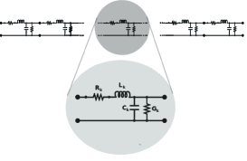
Fig. 1: Ladder network circuit topology (capacitors are nonlinear)

Inductors and capacitors are evidently the energy storage elements of the circuit, so we take as state variables the magnetic fluxes in the inductors, $\{\phi_{k}(t)\}_{k=1}^{N}$, and the charges on the capacitors, $\{Q_{k}\}_{k=1}^{N}$, with labels referring to the Stages $k=1,\ldots,N$, respectively, where they occur. The energy stored in the Stage $k$ (linear) inductor may be expressed in terms of its magnetic flux as $\frac{1}{2\,L_{0}}\phi_{k}^{2}$. To determine the energy stored in the nonlinear capacitors, note first that the charge on a capacitor may be expressed as a function of the voltage, $V$, held across the capacitor:

$$Q_{k}(V)=\int_{0}^{V}C(v)\,dv=C_{0}\,V_{0}\,\log\left(1+\frac{V}{V_{0}}\right),$$

which may be inverted to find

$$V_{k}(Q_{k})=V_{0}\,\left[\exp\left(\frac{Q_{k}}{C_{0}V_{0}}\right)-1\right].$$

The energy stored in the capacitor at Stage $k$ of the circuit, is then given by

$$\int_{0}^{Q_{k}}V_{k}(q)\,dq=C_{0}V_{0}^{2}\left[\exp\left(\frac{Q_{k}}{C_{0}V_{0}}\right)-1\right]-Q_{k}V_{0},$$

and the total energy stored in Stage $k$ is then

$$H^{[k]}(\phi_{k},Q_{k})=C_{0}V_{0}^{2}\left[\exp\left(\frac{Q_{k}}{C_{0}V_{0}}\right)-1\right]-Q_{k}V_{0}+\frac{1}{2\,L_{0}}\phi_{k}^{2}.$$

The Hamiltonian for this system is

$$H(Q_{1},\ldots,Q_{N},\phi_{1},\ldots,\phi_{N})=\sum_{k=1}^{N}H^{[k]}(\phi_{k},Q_{k}).$$

We order the state variables so that $\mathbf{x}=[Q_{1},\ldots,Q_{N},\phi_{1},\ldots,\phi_{N}]^{T}$ and therefore $\displaystyle\mathbf{J}=\left[\begin{array}[]{cc}\mathbf{0}&\mathsf{S}\\ -\mathsf{S}^{T}&\mathbf{0}\end{array}\right]$ where $\mathsf{S}$ is an upper bidiagonal matrix with $1$ on the diagonal and $-1$ on the superdiagonal; $\displaystyle\mathbf{R}=\left[\begin{array}[]{cc}G_{0}\mathbf{I}&\mathsf{0}\\ \mathsf{0}&R_{0}\mathbf{I}\end{array}\right]$; and $\displaystyle\mathbf{B}=\left[\mathbf{e}_{N+1},\mathbf{e}_{N}\right]$ where $\mathbf{e}_{k}$ denotes the $k^{th}$ column of the identity. Consider the particular case of a 50-stage ($N=50$) circuit with parameters: $L_{0}=2\mu\mathsf{H},\quad V_{0}=1\mathsf{V},\quad R_{0}=1\Omega,\quad G_{0}=10\mu\mho.$

We applied a voltage pulse to the left port of the network (Gaussian pulse windowed to 3$\mu$sec with a magnitude of 3V, $\sigma$ of $0.5$) and observed the output voltage at the right port. The output is displayed as a solid green trace in Figure 2. The induced response of the linearized full-order network is also displayed (green dashed line) for comparison. Notice that nonlinearity sharpens the peak of the response and significantly reduces dispersion. The pod basis sets are generated from uniformly sampled snapshots $\mathbf{x}(t)$ and $\nabla_{\mathbf{x}}H(\mathbf{x}(t))$ of this full-order system with Gaussian impulse training input. These basis sets are then used to construct the pod-ph reduced system. In the cases of $\mathcal{H}_{2}^{\varepsilon}$-phbases, the procedure described in Algorithm 2 is used. We also use Algorithm 3 to generate the pod-$\mathcal{H}_{2}^{\varepsilon}$-phbases. All three reduced models are then simulated for the same Gaussian impulse training input, which was used for generating the pod snapshot as well as a different one, a sinusoidal input. First we investigate the accuracy of pod-ph and $\mathcal{H}_{2}^{\varepsilon}$-ph for $r=6$. Figure 2 illustrates the two structure-preserving nonlinear reduced models capture the output of the original nonlinear system very accurately for both types of excitations.

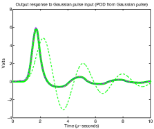
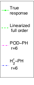
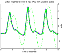
Fig. 2: Ladder network: Time responses of the reduced-order systems from Gaussian pulse (left) and from sinusoidal input(right).

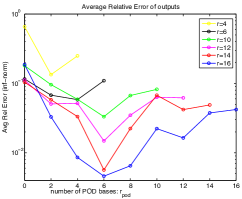
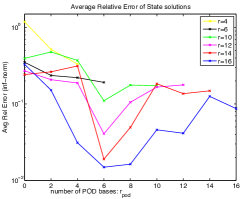
Fig. 3: Ladder Network: Average relative errors of outputs and state variables of structure-preserving reduced systems (8) using hybrid bases with different numbers of POD and $\mathcal{H}_{2}^{\Large\varepsilon}$vectors.

  

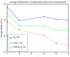
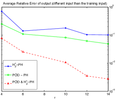
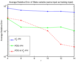
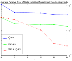
Fig. 4: Ladder Network: Average relative errors of outputs and state variables of reduced systems using bases from (i) $\mathcal{H}_{2}^{\Large\varepsilon}$, (ii) POD (iii) combination of POD and $\mathcal{H}_{2}^{\Large\varepsilon}$ (with same number of basis vectors for both POD and $\mathcal{H}_{2}^{\Large\varepsilon}$). The pod-ph reduced systems are constructed using Gaussian impulse training input. The top and the bottom plots, respectively, use the impulse input (same as the training input for POD) and with sinusoidal input (different from the training input for POD).

  

  

Next, we consider the effect on the accuracy of the state space solutions of using different proportions of pod-ph and $\mathcal{H}_{2}^{\varepsilon}$-ph basis vectors in the hybrid pod-$\mathcal{H}_{2}^{\varepsilon}$-ph basis. Results for a wide range of $r$ values are illustrated in Figure 3, depicting the relative error in the output. In these figures, the colors correspond to a fixed order $r$. The $x$-axis is the number of pod-ph basis vectors for that given order, so e.g., the blue line corresponds to relative error for $r=16$. For that line, the value corresponding to $x=12$ means that for the $r=16$ model, $\hat{r}=12$ pod-ph basis vectors are combined with $\bar{r}=r-\hat{r}=4$ $\mathcal{H}_{2}^{\varepsilon}$-ph basis vectors. The most accurate approximation resulted from reduced systems with bases that combined roughly equal numbers of pod-ph and $\mathcal{H}_{2}^{\varepsilon}$-ph basis vectors. Figure 4 shows that reduced systems constructed from these hybrid bases (using equal numbers of pod-ph and $\mathcal{H}_{2}^{\varepsilon}$-ph vectors) can give much more accurate approximations than those constructed with pod-ph alone or $\mathcal{H}_{2}^{\varepsilon}$-ph alone. For $r=12$, say, a reduced system with a hybrid basis using $\hat{r}=\bar{r}=6$ (red dashed line) produced roughly $10$ times smaller error for both state variables and outputs than those using only pod-ph (green solid lines) or $\mathcal{H}_{2}^{\varepsilon}$-ph bases (blue solid lines).

2.5 An a priori error bound for NLPH-reduced models

Fix a reduction order, $r$, and let ${\cal V}_{r}=\mathsf{Ran}(\mathbf{V}_{r})$ and ${\cal W}_{r}=\mathsf{Ran}(\mathbf{W}_{r})$ denote $r$-dimensional reduction subspaces used in creating reduced nlph systems as in (8). We provide an error analysis here that bounds the deviation between the true state trajectory of an nlph system and that provided by a reduced nlph system of the form given in (8). This leads in turn to a bound on the error between the true system output and the reduced nlph system output. Typically, the reduction subspaces ${\cal V}_{r}$ and ${\cal W}_{r}$ will be chosen consistently with the heuristics of (5) but the bounds we derive apply more generally.

Let $\mathbf{Q}\in\mathbb{R}^{n\times n}$ be a symmetric positive-definite matrix and define a weighted inner product on $\mathbb{R}^{n}$ as $\langle\mathbf{x},\mathbf{z}\rangle_{\mathbf{Q}}=\mathbf{x}^{T}\mathbf{Q}\mathbf{z}$, with a related norm, $\|\mathbf{x}\|_{\mathbf{Q}}=\sqrt{\langle\mathbf{x},\mathbf{x}\rangle_{\mathbf{Q}}}$. We leave the choice of $\mathbf{Q}$ open for the time being, however the choices $\mathbf{Q}=\mathbf{I}$ and $\mathbf{Q}=\nabla^{2}H(\mathbf{x}_{0})$ at a locally stable equilibrium point $\mathbf{x}_{0}$ will have particular merit.

For a mapping $\mathbf{F}:\mathbb{R}^{n}\to\mathbb{R}^{n}$, we define the associated Lipschitz constant and logarithmic Lipschitz constant of $\mathbf{F}$ relative to $\mathbf{Q}$ (see [26] ) as

$$L_{\mathbf{Q}}[\mathbf{F}]=\sup_{\mathbf{u}\neq\mathbf{v}}\frac{\|\mathbf{F}(\mathbf{u})-\mathbf{F}(\mathbf{v})\|_{\mathbf{Q}}}{\|\mathbf{u}-\mathbf{v}\|_{\mathbf{Q}}},\quad\mbox{and}\quad{\cal L}_{\mathbf{Q}}[\mathbf{F}]=\sup_{\mathbf{u}\neq\mathbf{v}}\frac{\langle\mathbf{u}-\mathbf{v},\mathbf{F}(\mathbf{u})-\mathbf{F}(\mathbf{v})\rangle_{\mathbf{Q}}}{\|\mathbf{u}-\mathbf{v}\|^{2}_{\mathbf{Q}}}$$ (18)

respectively. Note that ${\cal L}_{\mathbf{Q}}[\mathbf{F}]$ could be negative and $-L_{\mathbf{Q}}[\mathbf{F}]\leq{\cal L}_{\mathbf{Q}}[\mathbf{F}]\leq L_{\mathbf{Q}}[\mathbf{F}]$.

Suppose $\mathbf{Q}$-orthogonal bases for ${\cal V}_{r}$ and ${\cal W}_{r}$ are chosen: $\widetilde{\mathbf{V}}_{r},\widetilde{\mathbf{W}}_{r}\in\mathbb{R}^{n\times r}$ such that ${\cal V}_{r}=\mathsf{Ran}(\widetilde{\mathbf{V}}_{r})$ and ${\cal W}_{r}=\mathsf{Ran}(\widetilde{\mathbf{W}}_{r})$, with $\widetilde{\mathbf{V}}_{r}^{T}{\mathbf{Q}}\widetilde{\mathbf{V}}_{r}=\mathbf{I}$ and $\widetilde{\mathbf{W}}_{r}^{T}{\mathbf{Q}}\widetilde{\mathbf{W}}_{r}=\mathbf{I}$. Consider $\mathbf{Q}$-orthogonal projectors ${\boldsymbol{\Pi}}_{\cal V}:\mathbb{R}^{n}\to{\cal V}_{r}$, ${\boldsymbol{\Pi}}_{\cal W}:\mathbb{R}^{n}\to{\cal W}_{r}$ defined by ${\boldsymbol{\Pi}}_{\cal V}=\widetilde{\mathbf{V}}_{r}\widetilde{\mathbf{V}}_{r}^{T}{\mathbf{Q}}$ and ${\boldsymbol{\Pi}}_{\cal W}=\widetilde{\mathbf{W}}_{r}\widetilde{\mathbf{W}}_{r}^{T}{\mathbf{Q}}$. Define an ancillary state space projection as $\mbox{\boldmath${\mathcal{P}}$}_{r}=\mathbf{V}_{r}\mathbf{W}_{r}^{T}$. For a given (true) system trajectory, $\mathbf{x}(t)$, the best approximation (relative to the $\mathbf{Q}$-norm) that is available by a path in ${\cal V}_{r}$ is given by ${\boldsymbol{\Pi}}_{\cal V}\mathbf{x}(t)$, and so the state space error $\mathbf{x}(t)-\mathbf{V}_{r}\mathbf{x}_{r}(t)$ is bounded pointwise below as

$$\|(\mathbf{I}-{\boldsymbol{\Pi}}_{\cal V})\mathbf{x}(t)\|_{\mathbf{Q}}\leq\|\mathbf{x}(t)-\mathbf{V}_{r}\mathbf{x}_{r}(t)\|_{\mathbf{Q}}$$

for all $t\geq 0$. The error associated with the reduced internal force, $\nabla_{\mathbf{x}_{r}}H_{r}$, is bounded similarly

$$\|(\mathbf{I}-{\boldsymbol{\Pi}}_{\cal W})\nabla_{\mathbf{x}}H(\mathbf{x}(t))\|_{\mathbf{Q}}\leq\|\nabla_{\mathbf{x}}H(\mathbf{x}(t))-\mathbf{W}_{r}\nabla_{\mathbf{x}_{r}}H_{r}(\mathbf{x}_{r}(t))\|_{\mathbf{Q}}.$$

Let the optimal state-space and internal force residual vectors be defined as

$${\boldsymbol{\varepsilon}}_{\mathbf{x}}(t)=(\mathbf{I}-{\boldsymbol{\Pi}}_{\cal V})\mathbf{x}(t)\quad\mbox{and}\quad{\boldsymbol{\varepsilon}}_{\mathbf{F}}(t)=(\mathbf{I}-{\boldsymbol{\Pi}}_{\cal W})\nabla_{\mathbf{x}}H(\mathbf{x}(t)).$$

The squared residual state-space and internal force errors integrated over $[0,T]$ will be denoted as

$${\cal E}_{\mathbf{x}}=\int_{0}^{T}\|{\boldsymbol{\varepsilon}}_{\mathbf{x}}(t)\|^{2}_{\mathbf{Q}}\,dt=\int_{0}^{T}\|(\mathbf{I}-{\boldsymbol{\Pi}}_{\cal V})\mathbf{x}(t)\|^{2}_{\mathbf{Q}}\,dt$$

and

$${\cal E}_{\mathbf{F}}=\int_{0}^{T}\|{\boldsymbol{\varepsilon}}_{\mathbf{F}}(t)\|^{2}_{\mathbf{Q}}\,dt=\int_{0}^{T}\|(\mathbf{I}-{\boldsymbol{\Pi}}_{\cal W})\nabla_{\mathbf{x}}H(\mathbf{x}(t))\|^{2}_{\mathbf{Q}}\,dt.$$

We seek to bound the state space error, $\mathbf{x}-\mathbf{V}_{r}\mathbf{x}_{r}$, and output error, $\mathbf{y}-\mathbf{y}_{r}$, in terms of ${\cal E}_{\mathbf{x}}$, ${\cal E}_{\mathbf{F}}$, and the deviation between the projected and reduced initial condition. Note that when the reduction spaces, ${\cal V}_{r}$ and ${\cal W}_{r}$, are generated via a pod approach (e.g., Algorithm 1) then the aggregate errors ${\cal E}_{\mathbf{x}}$, ${\cal E}_{\mathbf{F}}$ are approximately minimized and can be expressed directly as the sum of neglected singular values of the snapshot matrix (either of $\mathbf{x}(t)$ or of $\nabla_{\mathbf{x}}H(\mathbf{x}(t))$. As we have seen in §2.4, the actual state space error or output error might not be minimized with this choice.

Theorem 2.

Suppose $\mathbf{Q}\in\mathbb{R}^{n\times n}$ is symmetric positive definite and that a reduced port-Hamiltonian system as in (8) is constructed to approximate the full order nlph system (1) using reduction bases $\mathbf{V}_{r}$, $\mathbf{W}_{r}\in\mathbb{R}^{n\times r}$ that are defined so that $\mathbf{V}_{r}^{T}{\mathbf{Q}}\mathbf{V}_{r}=\mathbf{I}_{r}$ and $\mathbf{V}_{r}^{T}\mathbf{W}_{r}=\mathbf{I}_{r}$. (Note that it may or may not be the case that $\mathbf{W}_{r}={\mathbf{Q}}\mathbf{V}_{r}$.) Suppose further that $\mathbf{F}(\mathbf{x})=\nabla_{\mathbf{x}}H(\mathbf{x})$ in (1) is Lipschitz continuous. Denote $\mbox{\boldmath${\mathcal{A}}$}=\mathbf{J}-\mathbf{R}$ and $\mbox{\boldmath${\mathcal{P}}$}_{r}=\mathbf{V}_{r}\mathbf{W}_{r}^{T}$. Then

$$\int_{0}^{T}\left\|\mathbf{x}(t)-\mathbf{V}_{r}\mathbf{x}_{r}(t)\right\|^{2}_{\mathbf{Q}}dt \leq C_{\mathbf{x}}\,{\cal E}_{\mathbf{x}}+C_{\mathbf{F}}\,{\cal E}_{\mathbf{F}}+C_{0}\mbox{\small$\|\mathbf{W}_{r}^{T}\mathbf{x}(0)-\mathbf{x}_{r}(0)\|^{2}$ }$$ (19)

$$\int_{0}^{T}\left\|\mathbf{y}(t)-\mathbf{y}_{r}(t)\right\|^{2}dt \leq \widehat{C}_{\mathbf{x}}{\cal E}_{\mathbf{x}}+\widehat{C}_{\mathbf{F}}{\cal E}_{\mathbf{F}}+\widehat{C}_{0}\mbox{\small$\|\mathbf{W}_{r}^{T}\mathbf{x}(0)-\mathbf{x}_{r}(0)\|^{2}$ }$$ (20)

where $\begin{array}[]{ccc}\alpha={\cal L}_{\mathbf{Q}}[\mbox{\boldmath${\mathcal{P}}$}_{r}\mbox{\boldmath${\mathcal{A}}$}\mbox{\boldmath${\mathcal{P}}$}_{r}^{T}\mathbf{F}],&\beta=\|\mbox{\boldmath${\mathcal{P}}$}_{r}\mbox{\boldmath${\mathcal{A}}$}\|_{\mathbf{Q}}\|\mbox{\boldmath${\mathcal{P}}$}_{r}^{T}\|_{\mathbf{Q}},&\gamma=L_{\mathbf{Q}}[\mathbf{F}]\ \|\mbox{\boldmath${\mathcal{P}}$}_{r}\|_{\mathbf{Q}},\end{array}$

$$\begin{array}[]{ccc}\delta=2\|\mathbf{B}^{T}{\mathbf{Q}}^{-1}\mathbf{B}\|\,\|\mbox{\boldmath${\mathcal{P}}$}_{r}^{T}\|_{\mathbf{Q}}^{2},&c_{\alpha}(t)=\int_{0}^{t}e^{2\alpha\tau}\,d\tau,&C_{\alpha}(t)=\int_{0}^{t}c_{\alpha}(\tau)\,d\tau,\end{array}$$

$$\begin{array}[]{ccc}C_{\mathbf{x}}=(2\beta\gamma)^{2}\,C_{\alpha}(T)+2\left\|\mbox{\boldmath${\mathcal{P}}$}_{r}\right\|^{2}_{\mathbf{Q}},&C_{\mathbf{F}}=(2\beta)^{2}\,C_{\alpha}(T),&C_{0}=2\,c_{\alpha}(T),\mbox{ and}\end{array}$$

$$\begin{array}[]{ccc}\widehat{C}_{\mathbf{x}}=\delta\cdot L_{\mathbf{Q}}[\mathbf{F}]^{2}C_{\mathbf{x}},&\widehat{C}_{\mathbf{F}}=\delta\cdot(1+L_{\mathbf{Q}}[\mathbf{F}]^{2}C_{\mathbf{F}}),&\widehat{C}_{0}=\delta\cdot L_{\mathbf{Q}}[\mathbf{F}]^{2}C_{0}.\end{array}$$

Proof.

First note that

$$(\mathbf{I}-\mbox{\boldmath${\mathcal{P}}$}_{r})\mathbf{x}(t) = (\mathbf{I}-\mbox{\boldmath${\mathcal{P}}$}_{r})(\mathbf{I}-{\boldsymbol{\Pi}}_{\cal V})\mathbf{x}(t)=(\mathbf{I}-\mbox{\boldmath${\mathcal{P}}$}_{r}){\boldsymbol{\varepsilon}}_{\mathbf{x}}(t)\quad\mbox{and}$$ (21)

$$(\mathbf{I}-\mbox{\boldmath${\mathcal{P}}$}_{r}^{T})\mathbf{F}(t) = (\mathbf{I}-\ \mbox{\boldmath${\mathcal{P}}$}_{r}^{T})(\mathbf{I}-{\boldsymbol{\Pi}}_{\cal W})\mathbf{F}(t)=(\mathbf{I}-\mbox{\boldmath${\mathcal{P}}$}_{r}^{T}){\boldsymbol{\varepsilon}}_{\mathbf{F}}(t).$$ (22)

The state space error can be separated into the sum of a component in $\mathsf{Ker}(\mbox{\boldmath${\mathcal{P}}$}_{r})$ (i.e., orthogonal to ${\cal W}_{r}$) and a component contained in $\mathsf{Ran}(\mbox{\boldmath${\mathcal{P}}$}_{r})={\cal V}_{r}$:

$$\mathbf{x}(t)-\mathbf{V}_{r}\mathbf{x}_{r}(t)={\boldsymbol{\rho}}(t)+\mathbf{V}_{r}{\boldsymbol{\theta}}(t),$$

where ${\boldsymbol{\rho}}(t)=\mathbf{x}(t)-\mathbf{V}_{r}\mathbf{W}_{r}^{T}\mathbf{x}(t)=(\mathbf{I}-\mbox{\boldmath${\mathcal{P}}$}_{r}){\boldsymbol{\varepsilon}}_{\mathbf{x}}(t)\in{\cal W}_{r}^{\perp}$ and ${\boldsymbol{\theta}}(t)=\mathbf{W}_{r}^{T}\mathbf{x}(t)-\mathbf{x}_{r}(t)$. Then

$$\int_{0}^{T}\|\mathbf{x}(t)-\mathbf{V}_{r}\mathbf{x}_{r}(t)\|_{\mathbf{Q}}^{2}\,dt\leq 2\int_{0}^{T}\|{\boldsymbol{\rho}}(t)\|_{\mathbf{Q}}^{2}\,dt+2\int_{0}^{T}\|{\boldsymbol{\theta}}(t)\|^{2}\,dt.$$ (23)

For the first term, we may estimate immediately

$$\int_{0}^{T}\|{\boldsymbol{\rho}}(t)\|_{\mathbf{Q}}^{2}\,dt\leq\int_{0}^{T}\|(\mathbf{I}-\mbox{\boldmath${\mathcal{P}}$}_{r}){\boldsymbol{\varepsilon}}_{\mathbf{x}}(t)\|_{\mathbf{Q}}^{2}\,dt\leq\|\mbox{\boldmath${\mathcal{P}}$}_{r}\|_{\mathbf{Q}}^{2}\ {\cal E}_{\mathbf{x}}$$

where we have made use of the identity, $\|\mathbf{I}-\mbox{\boldmath${\mathcal{P}}$}_{r}\|_{\mathbf{Q}}=\|\mbox{\boldmath${\mathcal{P}}$}_{r}\|_{\mathbf{Q}}$ (see [27]).

To bound the second term of (23), note that

$$\dot{{\boldsymbol{\theta}}}(t) = \mathbf{W}_{r}^{T}\dot{\mathbf{x}}(t)-\dot{\mathbf{x}}_{r}(t)=\mathbf{A}_{r}\mathbf{V}_{r}^{T}\left[\mathbf{F}(\mathbf{V}_{r}\mathbf{W}_{r}^{T}\mathbf{x}(t))-\mathbf{F}(\mathbf{V}_{r}\mathbf{x}_{r}(t))\right]+{\boldsymbol{\eta}}(t),$$

where $\mathbf{A}_{r}=\mathbf{J}_{r}-\mathbf{R}_{r}$ (see (15)) and ${\boldsymbol{\eta}}(t)=\mathbf{W}_{r}^{T}(\mathbf{J}-\mathbf{R})\left[\mathbf{F}(\mathbf{x}(t))-\mathbf{W}_{r}\mathbf{V}_{r}^{T}\mathbf{F}(\mathbf{V}_{r}\mathbf{W}_{r}^{T}\mathbf{x}(t))\right]$. Note that $\|{\boldsymbol{\theta}}(t)\|\,\frac{d}{dt}\|{\boldsymbol{\theta}}(t)\|=\frac{1}{2}\frac{d}{dt}\|{\boldsymbol{\theta}}(t)\|^{2}=\left\langle{\boldsymbol{\theta}}(t),\dot{{\boldsymbol{\theta}}}(t)\right\rangle$, so we have

$$\frac{d}{dt}\|{\boldsymbol{\theta}}(t)\|=\left\langle\frac{{\boldsymbol{\theta}}(t)}{\|{\boldsymbol{\theta}}(t)\|},\dot{{\boldsymbol{\theta}}}(t)\right\rangle=\left\langle\frac{{\boldsymbol{\theta}}(t)}{\|{\boldsymbol{\theta}}(t)\|},\mathbf{A}_{r}\mathbf{V}_{r}^{T}\left[\mathbf{F}(\mathbf{V}_{r}\mathbf{W}_{r}^{T}\mathbf{x}(t))-\mathbf{F}(\mathbf{V}_{r}\mathbf{x}_{r}(t))\right]+{\boldsymbol{\eta}}(t)\right\rangle.$$

Observe that

$$|\left\langle{\boldsymbol{\theta}}(t),{\boldsymbol{\eta}}(t)\right\rangle| =\left|\left\langle\mathbf{V}_{r}{\boldsymbol{\theta}}(t),\mathbf{V}_{r}\mathbf{W}_{r}^{T}(\mathbf{J}-\mathbf{R})\left[\mathbf{F}(\mathbf{x}(t))-\mathbf{W}_{r}\mathbf{V}_{r}^{T}\mathbf{F}(\mathbf{V}_{r}\mathbf{W}_{r}^{T}\mathbf{x}(t))\right]\right\rangle_{\mathbf{Q}}\right|$$

$$\leq\left\|\mathbf{V}_{r}{\boldsymbol{\theta}}(t)\right\|_{\mathbf{Q}}\ \|\mbox{\boldmath${\mathcal{P}}$}_{r}\mbox{\boldmath${\mathcal{A}}$}\left[\mathbf{F}(\mathbf{x}(t))-\mbox{\boldmath${\mathcal{P}}$}_{r}^{T}\mathbf{F}(\mbox{\boldmath${\mathcal{P}}$}_{r}\mathbf{x}(t))\right]\|_{\mathbf{Q}}$$

$$\leq\left\|{\boldsymbol{\theta}}(t)\right\|\|\mbox{\boldmath${\mathcal{P}}$}_{r}\mbox{\boldmath${\mathcal{A}}$}\|_{\mathbf{Q}}\|(\mathbf{I}-\mbox{\boldmath${\mathcal{P}}$}_{r}^{T})\mathbf{F}(\mathbf{x}(t))+\mbox{\boldmath${\mathcal{P}}$}_{r}^{T}(\mathbf{F}(\mathbf{x}(t))-\mathbf{F}(\mbox{\boldmath${\mathcal{P}}$}_{r}\mathbf{x}(t))\|_{\mathbf{Q}}$$

$$\leq\left\|{\boldsymbol{\theta}}(t)\right\|\|\mbox{\boldmath${\mathcal{P}}$}_{r}\mbox{\boldmath${\mathcal{A}}$}\|_{\mathbf{Q}}\cdot\left(\|(\mathbf{I}-\mbox{\boldmath${\mathcal{P}}$}_{r}^{T}){\boldsymbol{\varepsilon}}_{\mathbf{F}}(t)\|_{\mathbf{Q}}+\|\mbox{\boldmath${\mathcal{P}}$}_{r}^{T}\|_{\mathbf{Q}}\|\mathbf{F}(\mathbf{x}(t))-\mathbf{F}(\mbox{\boldmath${\mathcal{P}}$}_{r}\mathbf{x}(t))\|_{\mathbf{Q}}\right)$$

$$\leq\left\|{\boldsymbol{\theta}}(t)\right\|\|\mbox{\boldmath${\mathcal{P}}$}_{r}\mbox{\boldmath${\mathcal{A}}$}\|_{\mathbf{Q}}\cdot\left(\|\mathbf{I}-\mbox{\boldmath${\mathcal{P}}$}_{r}^{T}\|_{\mathbf{Q}}\|{\boldsymbol{\varepsilon}}_{\mathbf{F}}(t)\|_{\mathbf{Q}}+\|\mbox{\boldmath${\mathcal{P}}$}_{r}^{T}\|_{\mathbf{Q}}\ L_{\mathbf{Q}}[\mathbf{F}]\|(\mathbf{I}-\mbox{\boldmath${\mathcal{P}}$}_{r})\mathbf{x}(t)\|_{\mathbf{Q}}\right)$$

$$\leq\left\|{\boldsymbol{\theta}}(t)\right\|\left(\|\mbox{\boldmath${\mathcal{P}}$}_{r}\mbox{\boldmath${\mathcal{A}}$}\|_{\mathbf{Q}}\|\mbox{\boldmath${\mathcal{P}}$}_{r}^{T}\|_{\mathbf{Q}}\right)\cdot\left(\|{\boldsymbol{\varepsilon}}_{\mathbf{F}}(t)\|_{\mathbf{Q}}+L_{\mathbf{Q}}[\mathbf{F}]\ \|\mbox{\boldmath${\mathcal{P}}$}_{r}\|_{\mathbf{Q}}\|{\boldsymbol{\varepsilon}}_{\mathbf{x}}(t)\|_{\mathbf{Q}}\right)$$

$$\leq\left\|{\boldsymbol{\theta}}(t)\right\|\,\cdot\,\beta\left(\|{\boldsymbol{\varepsilon}}_{\mathbf{F}}(t)\|_{\mathbf{Q}}+\gamma\|{\boldsymbol{\varepsilon}}_{\mathbf{x}}(t)\|_{\mathbf{Q}}\right)$$

and

$$\left\langle{\boldsymbol{\theta}}(t),\mathbf{A}_{r}\mathbf{V}_{r}^{T}\left[\mathbf{F}(\mathbf{V}_{r}\mathbf{W}_{r}^{T}\mathbf{x}(t))-\mathbf{F}(\mathbf{V}_{r}\mathbf{x}_{r}(t))\right]\right\rangle$$

$$\qquad\qquad=\left\langle\mathbf{V}_{r}{\boldsymbol{\theta}}(t),\mbox{\boldmath${\mathcal{P}}$}_{r}\mbox{\boldmath${\mathcal{A}}$}\mbox{\boldmath${\mathcal{P}}$}_{r}^{T}\left[\mathbf{F}(\mathbf{V}_{r}\mathbf{W}_{r}^{T}\mathbf{x}(t))-\mathbf{F}(\mathbf{V}_{r}\mathbf{x}_{r}(t))\right]\right\rangle_{\mathbf{Q}}$$

$$\qquad\qquad\qquad\leq{\cal L}_{\mathbf{Q}}[\mbox{\boldmath${\mathcal{P}}$}_{r}\mbox{\boldmath${\mathcal{A}}$}\mbox{\boldmath${\mathcal{P}}$}_{r}^{T}\mathbf{F}]\,\cdot\,\left\|\mathbf{V}_{r}{\boldsymbol{\theta}}(t)\right\|_{\mathbf{Q}}^{2}=\alpha\,\left\|{\boldsymbol{\theta}}(t)\right\|^{2},$$

where we make use of the fact that $\|\mathbf{I}-\mbox{\boldmath${\mathcal{P}}$}_{r}\|_{\mathbf{Q}}=\|\mbox{\boldmath${\mathcal{P}}$}_{r}\|_{\mathbf{Q}}$ and $\|\mathbf{I}-\mbox{\boldmath${\mathcal{P}}$}_{r}^{T}\|_{\mathbf{Q}}=\|\mbox{\boldmath${\mathcal{P}}$}_{r}^{T}\|_{\mathbf{Q}}$.

For (20), we find

$$\|\mathbf{y}-\mathbf{y}_{r}\| =\|\mathbf{B}^{T}\mathbf{F}(\mathbf{x})-\mathbf{B}^{T}\mathbf{W}_{r}\mathbf{V}_{r}^{T}\mathbf{F}(\mathbf{V}_{r}\mathbf{x}_{r})\|$$

$$=\|\mathbf{B}^{T}{\mathbf{Q}}^{-1/2}{\mathbf{Q}}^{1/2}\left(\mathbf{F}(\mathbf{x})-\mbox{\boldmath${\mathcal{P}}$}_{r}^{T}\mathbf{F}(\mathbf{V}_{r}\mathbf{x}_{r})\right)\|$$

$$\leq\|\mathbf{B}^{T}{\mathbf{Q}}^{-1/2}\|\,\|(\mathbf{I}-\mbox{\boldmath${\mathcal{P}}$}_{r}^{T}){\boldsymbol{\varepsilon}}_{\mathbf{F}}+\mbox{\boldmath${\mathcal{P}}$}_{r}^{T}\left(\mathbf{F}(\mathbf{x})-\mathbf{F}(\mathbf{V}_{r}\mathbf{x}_{r})\right)\|_{\mathbf{Q}}$$

$$\leq\|\mathbf{B}^{T}{\mathbf{Q}}^{-1}\mathbf{B}\|^{1/2}\left(\|(\mathbf{I}-\mbox{\boldmath${\mathcal{P}}$}_{r}^{T}){\boldsymbol{\varepsilon}}_{\mathbf{F}}\|_{\mathbf{Q}}+\|\mbox{\boldmath${\mathcal{P}}$}_{r}^{T}\left(\mathbf{F}(\mathbf{x})-\mathbf{F}(\mathbf{V}_{r}\mathbf{x}_{r})\right)\|_{\mathbf{Q}}\right)$$

$$\leq\|\mathbf{B}^{T}{\mathbf{Q}}^{-1}\mathbf{B}\|^{1/2}\,\|\mbox{\boldmath${\mathcal{P}}$}_{r}^{T}\|_{\mathbf{Q}}\left(\|{\boldsymbol{\varepsilon}}_{\mathbf{F}}\|_{\mathbf{Q}}+\|\left(\mathbf{F}(\mathbf{x})-\mathbf{F}(\mathbf{V}_{r}\mathbf{x}_{r})\right)\|_{\mathbf{Q}}\right)$$

$$\leq\|\mathbf{B}^{T}{\mathbf{Q}}^{-1}\mathbf{B}\|^{1/2}\,\|\mbox{\boldmath${\mathcal{P}}$}_{r}^{T}\|_{\mathbf{Q}}\left(\|{\boldsymbol{\varepsilon}}_{\mathbf{F}}\|_{\mathbf{Q}}+L_{\mathbf{Q}}[\mathbf{F}]\|\mathbf{x}-\mathbf{V}_{r}\mathbf{x}_{r}\|_{\mathbf{Q}}\right)$$

Thus,

$$\int_{0}^{T}\|\mathbf{y}(t)-\mathbf{y}_{r}(t)\|^{2}\,dt \leq 2\|\mathbf{B}^{T}{\mathbf{Q}}^{-1}\mathbf{B}\|\,\|\mbox{\boldmath${\mathcal{P}}$}_{r}^{T}\|_{\mathbf{Q}}^{2}\int_{0}^{T}\left(\|{\boldsymbol{\varepsilon}}_{\mathbf{F}}(t)\|_{\mathbf{Q}}^{2}+L_{\mathbf{Q}}[\mathbf{F}]^{2}\|\mathbf{x}-\mathbf{V}_{r}\mathbf{x}_{r}\|_{\mathbf{Q}}^{2}\right)\,dt$$

$$\leq 2\|\mathbf{B}^{T}{\mathbf{Q}}^{-1}\mathbf{B}\|\,\|\mbox{\boldmath${\mathcal{P}}$}_{r}^{T}\|_{\mathbf{Q}}^{2}\ \cdot$$

$$\qquad\qquad\left({\cal E}_{\mathbf{F}}+L_{\mathbf{Q}}[\mathbf{F}]^{2}\left(C_{\mathbf{x}}\,{\cal E}_{\mathbf{x}}+C_{\mathbf{F}}\,{\cal E}_{\mathbf{F}}+C_{0}\mbox{\small$\|\mathbf{W}_{r}^{T}\mathbf{x}(0)-\mathbf{x}_{r}(0)\|^{2}$ }\right)\right)$$

and (20) follows. ∎

3 Structure-preserving model reduction with DEIM

The performance of projection-based reduels of nonlinear systems can be degraded by the need to lift the reduced state to the full state dimension in order to evaluate the nonlinear term. For example, consider the evaluation of $\mathbf{V}_{r}^{T}\nabla_{\!\mathbf{x}}{H}(\mathbf{V}_{r}\mathbf{x}_{r})$ in (6). If $\nabla_{\!\mathbf{x}}{H}(\mathbf{x})$ is nonlinear in $\mathbf{x}$, it is likely that $\mathbf{V}_{r}^{T}\nabla_{\!\mathbf{x}}{H}(\mathbf{V}_{r}\mathbf{x}_{r})$ cannot be precomputed explicitly as a map from $\mathbb{R}^{r}$ to $\mathbb{R}^{r}$ without an intermediate lifting to $\mathbb{R}^{n}$. The order of complexity required to evolve the reduced system will then remain at least $\mathcal{O}(n)$ and there may be little benefit seen in the use of a reduced model. Several approaches have been proposed to address this difficulty; see, e.g., [1, 2, 4, 6, 9]. We resolve the complexity issue by developing a variant of the discrete empirical interpolation method (deim) [6], which is itself a discrete variant of the Empirical Interpolation Method introduced in [2]. Since deim (as presented in [6]) does not typically preserve port-Hamiltonian structure, we develop here a structure-preserving variant of deim together with associated error estimates. There have been other structure-preserving methods developed recently that employ methods resolving the lifting bottleneck, e.g., see [5] for an approach that preserves Lagrangian structure in structural dynamics using gappy POD.

3.1 The Discrete Empirical Interpolation Method

The ‘lifting bottleneck’ in the reduction of large scale nonlinear models as described above is resolved by deim through the approximation of the nonlinear system function via interpolation. This approximation is done in such a way as to not require a prolongation of the reduced state variables (‘lifting’) back to the original high dimensional state space. Only a few selected entries of the original nonlinear term need be evaluated at each time step.

In particular, let $\mathbf{f}:\mathscr{D}\mapsto\mathbb{R}^{n}$ be a nonlinear vector-valued function defined on a domain $\mathscr{D}\subseteq\mathbb{R}^{n}$. Let $\mathbf{U}_{m}=[\mathbf{u}_{1},\dots,\mathbf{u}_{m}]\in\mathbb{R}^{n\times m}$ have rank $m$ and define $\mathbf{E}_{m}=[\mathbf{e}_{\wp_{1}},\dots,\mathbf{e}_{\wp_{m}}]\in\mathbb{R}^{n\times m}$ with the index set $\{\wp_{1},\dots,\wp_{m}\}$ output from Algorithm 4 using the input basis $\{\mathbf{u}_{i}\}_{i=1}^{m}$. $\mathbf{e}_{\wp_{j}}\in\mathbb{R}^{n}$ denotes the $\wp_{j}$th column of the $n$-by-$n$ identity matrix.

The deim approximation of order $m\leq n$ for $\mathbf{f}$ in ${\rm span}\{\mathbf{U}_{m}\}$ is given by

$$\widehat{\mathbf{f}}(\tau):=\mathbb{P}\,\mathbf{f}(\tau),\quad\mbox{ where }\quad\mathbb{P}=\mathbf{U}_{m}(\mathbf{E}_{m}^{T}\mathbf{U}_{m})^{-1}\mathbf{E}_{m}^{T}.$$ (24)

Note that in the original work, [6], $\mathbf{U}_{m}$ is assumed to have orthonormal columns, yet linear independence suffices for $\mathbb{P}$ to be well defined and that is all that we require here.

Algorithm 4 : deim [6]

INPUT: $\{\mathbf{u}_{\ell}\}_{\ell=1}^{m}\subset\mathbb{R}^{n}$ linearly independent
OUTPUT: $\vec{\wp}=[\wp_{1},\dots,\wp_{m}]^{T}\in\mathbb{R}^{m}$

1:   $[|\rho|,\hskip 5.69054pt\wp_{1}]={\tt max}\{|\mathbf{u}_{1}|\}$

2:  $\mathbf{U}=[\mathbf{u}_{1}]$, $\mathbf{E}=[\mathbf{e}_{\wp_{1}}]$, $\vec{\wp}=[\wp_{1}]$

3:  for $\ell=2$ to $m$ do

4:      Solve $(\mathbf{E}^{T}\mathbf{U})\mathbf{c}=\mathbf{E}^{T}\mathbf{u}_{\ell}$ for $\mathbf{c}$

5:      $\mathbf{r}=\mathbf{u}_{\ell}-\mathbf{U}\mathbf{c}$

6:      $[|\rho|,\hskip 5.69054pt\wp_{\ell}]={\tt max}\{|\mathbf{r}|\}$  $\left(\begin{array}[]{c}\mbox{ $|\rho|=|v_{{\wp}}|=\max_{i=1,\dots,n}\{|v_{i}|\}$, with the}\\ \mbox{smallest index taken for $\wp$ in case of ties.}\end{array}\right)$

7:      $\mathbf{U}\leftarrow[\mathbf{U}\hskip 5.69054pt\mathbf{u}_{\ell}]$, $\mathbf{E}\leftarrow[\mathbf{E}\hskip 5.69054pt\mathbf{e}_{\wp_{\ell}}]$, $\vec{\wp}\leftarrow\left[\begin{array}[]{c}\vec{\wp}\\ \wp_{\ell}\end{array}\right]$

8:  end for

We adapt an error bound for the deim function approximation derived in [6] for the case that $\mathbf{U}_{m}$ has $\mathbf{Q}$-orthonormal columns.

Lemma 3.

If $\mathbf{U}_{m}^{T}\mathbf{Q}\mathbf{U}_{m}=\mathbf{I}_{m}$, then $\|\mathbf{f}(\tau)-\widehat{\mathbf{f}}(\tau)\|_{\mathbf{Q}}\leq\|\mathbb{P}\|_{\mathbf{Q}}\,\hskip 2.84526pt\mathscr{E}_{\mathbf{Q}}(\mathbf{f}(\tau),\mathbf{U}_{m})$, where $\mathscr{E}_{\mathbf{Q}}(\mathbf{f}(\tau),\mathbf{U}_{m})$ is the best $\mathbf{Q}$-norm approximation error for $\mathbf{f}(\tau)$ from $\mathsf{Ran}(\mathbf{U}_{m})$.

The invertibility of $\mathbf{E}^{T}\mathbf{U}$ at the end of each cycle of the deim procedure is verified in [6] where it is shown that each deim interpolation index is selected in order to limit the stepwise growth of the factor $\|(\mathbf{E}_{m}^{T}\mathbf{U}_{m})^{-1}\|=\|\mathbb{P}\|_{\mathbf{Q}}$ in the error bound. This will be used in the next section to assess the accuracy of the state variables in the deim reduced system. deim shown in Algorithm 4 uses LU with partial pivoting for interpolation indices. A new selection operator for deim based on the pivoted QR has been recently introduced by Drmač and Gugercin [7]. Our numerical results in this paper are based the original implementation in Algorithm 4. We also refer the reader to [17] for a recently introduced localized version of deim and to [18] for online adaptivity approach to deim that adjusts the deim subspace and the interpolation indices with online low-rank updates.

Consider the nonlinear ph system in (1) where $\mathbf{J}$, $\mathbf{R}$, and $\mathbf{B}$ are constant, and $\mathbf{F}(\mathbf{x})=\nabla_{\mathbf{x}}H(\mathbf{x})$ is nonlinear. In the reduced system (8), we use the approximation (7): $\nabla_{\mathbf{x}}H(\mathbf{x})\approx\mathbf{W}_{r}\mathbf{V}_{r}^{T}\nabla_{\mathbf{x}}H(\mathbf{x})$, for $\mathbf{x}\in\mathsf{Ran}(\mathbf{V}_{r})$. deim can be applied directly to $\mathbf{F}$ (using $\mathbf{W}_{r}$ instead of $\mathbf{U}$) to obtain an approximation in the form of

$$\mathbf{F}(\mathbf{V}_{r}\mathbf{x}_{r})\approx\mathbf{W}_{r}(\mathbf{E}^{T}\mathbf{W}_{r})^{-1}\mathbf{E}^{T}\mathbf{F}(\mathbf{V}_{r}\mathbf{x}_{r}),$$

allowing us to evaluate the nonlinear term with low complexity. However, this approach will not preserve the underlying ph structure; it generally will not produce a passive system; and indeed, the reduced system might no longer be stable. We modify deim to overcome these shortcomings.

3.2 The DEIM Hamiltonian

We continue to assume that the source of nonlinearity in the system (1) lies in the Hamiltonian gradient: $\nabla_{\mathbf{x}}H(\mathbf{x})$, and we focus on approximating this nonlinear term in a way that is consistent with the ph structure, so that the complexity does not depend on the original full-order dimension. This restriction comes largely without loss of generality since additional state-space dependence of $\mathbf{J}$, $\mathbf{R}$, and $\mathbf{B}$ can be accommodated with usual deim-based approaches with no threat to the underlying port-Hamiltonian structure.

We first identify a linear component of $\nabla_{\mathbf{x}}H(\mathbf{x})$, or equivalently, a quadratic component of $H(\mathbf{x})$:

$$H(\mathbf{x})=\mbox{$\frac{1}{2}$}\mathbf{x}^{T}\mathbf{Q}\mathbf{x}+h(\mathbf{x})$$ (25)

where $\mathbf{Q}$ is an $n\times n$ positive-definite, constant matrix. A typical choice may be $\mathbf{Q}=\nabla^{2}_{\mathbf{x}}H(\mathbf{x}_{0})$ at an equilibrium point, $\nabla_{\mathbf{x}}H(\mathbf{x}_{0})={\bf 0}$. Similar strategies are considered in [15] to maintain high accuracy. Once $\mathbf{Q}$ is selected, (25) determines $h(\mathbf{x})$ and $\nabla_{\mathbf{x}}h(\mathbf{x})$ then captures the remaining nonlinear portion of $\nabla_{\mathbf{x}}H(\mathbf{x})$.

We select a new modeling basis, $\mathbf{U}_{m}$, orthogonalized with respect to $\mathbf{Q}$, so that $\nabla_{\mathbf{x}}h(\mathbf{x}(t))\approx\mathbf{U}_{m}\mathbf{g}_{m}(t)$ and $\mathbf{U}_{m}^{T}\mathbf{Q}\mathbf{U}_{m}=\mathbf{I}$. There will be a variety of choices for $\mathbf{U}_{m}$; we consider a couple of them below. Using $\mathbf{U}_{m}$, we calculate deim indices, $\wp_{1},\dots,\wp_{m}$ with Algorithm 4, define the associated deim projection, $\mathbb{P}=\mathbf{U}_{m}(\mathbf{E}_{m}^{T}\mathbf{U}_{m})^{-1}\mathbf{E}_{m}^{T}$, and finally, introduce a “deim Hamiltonian”:

$$\widehat{H}(\mathbf{x})=\frac{1}{2}\,\mathbf{x}^{T}\,\mathbf{Q}\,\mathbf{x}\,+\,h(\mathbb{P}^{T}\mathbf{x}).$$ (26)

Observe that $\nabla_{\mathbf{x}}\widehat{H}(\mathbf{x})=\mathbf{Q}\mathbf{x}+\mathbb{P}\nabla_{\mathbf{x}}h(\mathbb{P}^{T}\mathbf{x})$, so the error induced by $\nabla_{\mathbf{x}}\widehat{H}(\mathbf{x})$ is

$$\nabla_{\mathbf{x}}H(\mathbf{x})-\nabla_{\mathbf{x}}\widehat{H}(\mathbf{x})=\nabla_{\mathbf{x}}h(\mathbf{x})-\mathbb{P}\nabla_{\mathbf{x}}h(\mathbb{P}^{T}\mathbf{x}).$$

If $\mathbf{Q}$ is chosen well then $\nabla_{\mathbf{x}}\widehat{H}(\mathbf{x})$ can exactly recover the “linear part” of $\nabla_{\mathbf{x}}H(\mathbf{x})$. Observe that the evaluation of the remaining nonlinear term, $\mathbb{P}\nabla_{\mathbf{x}}h(\mathbb{P}^{T}\mathbf{x})$, only involves the evaluation of $m$ elements of $\nabla_{\mathbf{x}}h$ on only $m$ nonzero arguments - the remaining arguments having only $m$ nonzero values.

Observe that trivially $\nabla_{\mathbf{x}}H(\mathbf{x})=\nabla_{\mathbf{x}}\widehat{H}(\mathbf{x})$ when $m=n$. However, the approximation $\nabla_{\mathbf{x}}H(\mathbf{x})\approx\nabla_{\mathbf{x}}\widehat{H}(\mathbf{x})$ can be effective even for significantly smaller $m\ll n$. Nonetheless, the enforced symmetry in this approximation appears to require some additional considerations.

Let $\Omega\subset\mathbb{R}^{n}$, be a compact convex set containing each of the trajectories $\mathbf{x}(t)$ and $\mathbb{P}^{T}\mathbf{x}(t)$, for $0\leq t\leq T$ on its interior. Define

$$\mathbf{K}^{\circ}=\int_{\Omega}\nabla_{\mathbf{x}}h(\mathbf{x})\nabla_{\mathbf{x}}h(\mathbf{x})^{T}\mathbf{Q}\ d\nu(\mathbf{x}).$$

$\mathbf{K}^{\circ}$ is $\mathbf{Q}$-selfadjoint and positive-definite with associated eigenpairs $\mathbf{K}^{\circ}\,\mathbf{u}_{k}^{\circ}=\sigma_{k}^{\circ}\,\mathbf{u}_{k}^{\circ}$ for $\sigma_{1}^{\circ}\geq\sigma_{2}^{\circ}\geq\ldots\geq\sigma_{n}^{\circ}\geq 0$ and $\mathbf{Q}$-orthonormal eigenvectors, $\mathbf{u}_{i}^{\circ T}\mathbf{Q}\mathbf{u}_{j}^{\circ}=\delta_{ij}$. For any choice of $0<m\leq n$, designate the dominant modes as $\mathbf{U}_{m}^{\circ}=[\mathbf{u}_{1}^{\circ},\,\ldots,\,\mathbf{u}_{m}^{\circ}]$ and the complementary subdominant modes as $\widetilde{\mathbf{U}}_{m}^{\circ}=[\mathbf{u}_{m+1}^{\circ},\,\ldots,\,\mathbf{u}_{n}^{\circ}]$. Observe that if $\Omega$ shrank to $\mathbf{x}(t)$, $\mathbf{U}_{m}^{\circ}$ could be considered as the limiting case of a usual POD basis of dimension $m$.

We have in that case,

$$\mathbf{K}^{\circ}\,\mathbf{U}_{m}^{\circ}=\mathbf{U}_{m}^{\circ}\mathsf{diag}(\sigma_{1}^{\circ},\,\sigma_{2}^{\circ},\,\ldots,\,\sigma_{m}^{\circ})\quad\mbox{and}\quad\mathbf{K}^{\circ}\,\widetilde{\mathbf{U}}_{m}^{\circ}=\widetilde{\mathbf{U}}_{m}^{\circ}\mathsf{diag}(\sigma_{m+1}^{\circ},\,\ldots,\,\sigma_{n}^{\circ}).$$

If $\mathscr{E}_{\mathbf{Q}}(\nabla_{\mathbf{x}}h(\mathbf{x}),\mathbf{U}_{m}^{\circ})$ denotes the (local) best $\mathbf{Q}$-norm approximation error to $\nabla_{\mathbf{x}}h(\mathbf{x})$ out of $\mathbf{U}_{m}^{\circ}$ (as defined in Lemma 3), then

$$\left(\varepsilon_{\mathbf{Q}}^{\circ(m)}\right)^{2}=\int_{\Omega}\mathscr{E}_{\mathbf{Q}} (\nabla_{\mathbf{x}}h(\mathbf{x}),\mathbf{U}_{m}^{\circ})^{2}\,d\nu(\mathbf{x})=\int_{\Omega}\|(\mathbf{I}-\mathbf{U}_{m}^{\circ}\mathbf{U}_{m}^{\circ T}\mathbf{Q})\nabla_{\mathbf{x}}h(\mathbf{x})\|_{\mathbf{Q}}^{2}\ d\nu(\mathbf{x})$$

$$=\int_{\Omega} \mathsf{trace}\left((\mathbf{I}-\mathbf{U}_{m}^{\circ}\mathbf{U}_{m}^{\circ T}\mathbf{Q})\nabla_{\mathbf{x}}h(\mathbf{x})\nabla_{\mathbf{x}}h(\mathbf{x})^{T}(\mathbf{I}-\mathbf{Q}\mathbf{U}_{m}^{\circ}\mathbf{U}_{m}^{\circ T})\mathbf{Q}\right)\,d\nu(\mathbf{x})$$

$$= \int_{\Omega}\mathsf{trace}\left(\nabla_{\mathbf{x}}h(\mathbf{x})\nabla_{\mathbf{x}}h(\mathbf{x})^{T}\mathbf{Q}(\mathbf{I}-\mathbf{U}_{m}^{\circ}\mathbf{U}_{m}^{\circ T}\mathbf{Q})\right)\ d\nu(\mathbf{x})$$

$$=\mathsf{trace}\left(\mathbf{K}^{\circ}(\mathbf{I}-\mathbf{U}_{m}^{\circ}\mathbf{U}_{m}^{\circ T}\mathbf{Q})\right)=\sum_{k=m+1}^{n}\sigma_{k}^{\circ}.$$

Lemma 4.

Suppose $h(\mathbf{x})$ is continuously differentiable in $\Omega$. Construct the DEIM projection using $\mathbf{U}_{m}^{\circ}$ with $\mathbb{P}_{\circ}=\mathbf{U}_{m}^{\circ}(\mathbf{E}_{m}^{T}\mathbf{U}_{m}^{\circ})^{-1}\mathbf{E}_{m}^{T}$. Then

$$|h(\mathbf{x})-h(\mathbb{P}_{\circ}^{T}\mathbf{x})|\leq\|(\mathbf{I}-\mathbb{P}_{\circ}^{T})\mathbf{x}(t)\|_{\mathbf{Q}^{-1}}\cdot\varepsilon_{\mathbf{Q}}^{\circ(m)}$$ (27)

Proof.

Define the columns of $\widetilde{\mathbf{E}}_{m}$ to be complementary to those of $\mathbf{E}_{m}$ so that $[\mathbf{E}_{m},\widetilde{\mathbf{E}}_{m}]$ is an $n\times n$ permutation matrix. Observe that $\mathsf{Ran}(\mathbb{P}_{\circ}^{T})=\mathsf{Ran}(\mathbf{E}_{m})$ and $\mathsf{Ran}(\mathbf{I}-\mathbb{P}_{\circ}^{T})=\mathsf{Ker}(\mathbb{P}_{\circ}^{T})=\mathsf{Ker}(\mathbf{U}_{m}^{\circ T})=\mathsf{Ran}(\mathbf{Q}\widetilde{\mathbf{U}}_{m}^{\circ})$. Hence,

$$\mathbf{x}=\mathbb{P}_{\circ}^{T}\mathbf{x}+(\mathbf{I}-\mathbb{P}_{\circ}^{T})\mathbf{x}=\mathbf{E}_{m}{\boldsymbol{\zeta}}_{1}+\mathbf{Q}\widetilde{\mathbf{U}}_{m}^{\circ}{\boldsymbol{\zeta}}_{2}$$

for continuous functions given as

$${\boldsymbol{\zeta}}_{1}(\mathbf{x})=(\mathbf{U}_{m}^{\circ T}\mathbf{E}_{m})^{-1}\mathbf{U}_{m}^{\circ T}\mathbf{x}\quad\mbox{ and }\quad{\boldsymbol{\zeta}}_{2}(\mathbf{x})=(\widetilde{\mathbf{E}}_{m}^{T}\mathbf{Q}\widetilde{\mathbf{U}}_{m}^{\circ})^{-1}\widetilde{\mathbf{E}}_{m}^{T}\mathbf{x}.$$

Note that, $\mathbf{Q}^{\frac{1}{2}}\widetilde{\mathbf{U}}_{m}^{\circ}{\boldsymbol{\zeta}}_{2}=\mathbf{Q}^{-\frac{1}{2}}(\mathbf{I}-\mathbb{P}_{\circ}^{T})\mathbf{x}$ and $\|{\boldsymbol{\zeta}}_{2}\|=\|(\mathbf{I}-\mathbb{P}_{\circ}^{T})\mathbf{x}\|_{\mathbf{Q}^{-1}}$.

For each fixed $\mathbf{x}\in\Omega$, define the path connecting $\mathbf{x}$ and $\mathbb{P}_{\circ}^{T}\mathbf{x}$:

$$\mathcal{C}(\mathbf{x})=\{\theta\mathbf{x}+(1-\theta)\mathbb{P}_{\circ}^{T}\mathbf{x}\left|\ \theta\in[0,1]\right.\}=\{\mathbf{E}_{m}{\boldsymbol{\zeta}}_{1}+\theta\,\mathbf{Q}\widetilde{\mathbf{U}}_{m}^{\circ}{\boldsymbol{\zeta}}_{2}\left|\ \theta\in[0,1]\right.\}.$$

If we define, $f({\boldsymbol{\zeta}}_{1},{\boldsymbol{\zeta}}_{2})=h(\mathbf{x})=h(\mathbf{E}_{m}{\boldsymbol{\zeta}}_{1}+\widetilde{\mathbf{U}}_{m}^{\circ}{\boldsymbol{\zeta}}_{2})$, observe that

$$\nabla_{{\boldsymbol{\zeta}}_{2}}f({\boldsymbol{\zeta}}_{1},{\boldsymbol{\zeta}}_{2})=\widetilde{\mathbf{U}}_{m}^{\circ T}\mathbf{Q}\nabla_{\mathbf{x}}h(\mathbf{E}_{m}{\boldsymbol{\zeta}}_{1}+\mathbf{Q}\widetilde{\mathbf{U}}_{m}^{\circ}.{\boldsymbol{\zeta}}_{2}).$$

Integrating $\nabla_{{\boldsymbol{\zeta}}_{2}}f$ along $\mathcal{C}(t)$, we find

$$|h(\mathbf{x})-h(\mathbb{P}_{\circ}^{T}\mathbf{x})|= |f({\boldsymbol{\zeta}}_{1},{\boldsymbol{\zeta}}_{2})-f({\boldsymbol{\zeta}}_{1},0)|=\left|\int_{\mathcal{C}(\mathbf{x})}\widetilde{\mathbf{U}}_{m}^{\circ T}\mathbf{Q}\nabla_{\mathbf{x}}h({\boldsymbol{\xi}})\,\cdot\,d{\boldsymbol{\xi}}\right|$$

$$= \left|\int_{0}^{1}{\boldsymbol{\zeta}}_{2}^{T}\widetilde{\mathbf{U}}_{m}^{\circ T}\mathbf{Q}\nabla_{\mathbf{x}}h(\mathbf{E}_{m}{\boldsymbol{\zeta}}_{1}+\theta\,\mathbf{Q}\widetilde{\mathbf{U}}_{m}^{\circ}{\boldsymbol{\zeta}}_{2})\,d\theta\right|$$

$$= \|{\boldsymbol{\zeta}}_{2}\|\left(\int_{0}^{1}\|\widetilde{\mathbf{U}}_{m}^{\circ T}\mathbf{Q}\nabla_{\mathbf{x}}h(\mathbf{E}_{m}{\boldsymbol{\zeta}}_{1}+\theta\,\mathbf{Q}\widetilde{\mathbf{U}}_{m}^{\circ}{\boldsymbol{\zeta}}_{2})\|^{2}\,d\theta\right)^{\!\frac{1}{2}}$$

$$\leq \|{\boldsymbol{\zeta}}_{2}\|\left(\int_{\Omega}\|\widetilde{\mathbf{U}}_{m}^{\circ T}\mathbf{Q}\nabla_{\mathbf{x}}h({\boldsymbol{\xi}})\|^{2}\ d\nu({\boldsymbol{\xi}})\right)^{\!\frac{1}{2}}$$

$$\leq \|(\mathbf{I}-\mathbb{P}_{\circ}^{T})\mathbf{x}(t)\|_{\mathbf{Q}^{-1}}\cdot\varepsilon_{\mathbf{Q}}^{\circ(m)}.$$

∎

Thus, a modest extension of the usual POD basis is sufficient to produce DEIM approximations and associated DEIM Hamiltonians that converge uniformly to the true Hamiltonian with a rate related to the decay rate of $\sigma_{k}^{\circ}$. Stronger hypotheses on the approximating modes appear to be necessary in order to assure rapid convergence of the corresponding gradients. Towards that end, we assume that $h$ is twice continuously differentiable and define

$$\mathbf{K}=\int_{\Omega}\nabla_{\mathbf{x}}h(\mathbf{x})\nabla_{\mathbf{x}}h(\mathbf{x})^{T}\mathbf{Q}\ d\nu(\mathbf{x})+\int_{\Omega}\left(\nabla_{\mathbf{x}}^{2}h(\mathbf{x})\right)^{2}\,\mathbf{Q}\ d\nu(\mathbf{x}).$$

$\mathbf{K}$ is $\mathbf{Q}$-selfadjoint and positive-definite with associated eigenpairs $\mathbf{K}\,\mathbf{u}_{k}=\sigma_{k}\,\mathbf{u}_{k}$ for $\sigma_{1}\geq\sigma_{2}\geq\ldots\geq\sigma_{n}\geq 0$ and $\mathbf{Q}$-orthonormal eigenvectors, $\mathbf{u}_{i}^{T}\mathbf{Q}\mathbf{u}_{j}=\delta_{ij}$. Analogous to what has gone before, designate dominant modes as $\mathbf{U}_{m}=[\mathbf{u}_{1},\,\ldots,\,\mathbf{u}_{m}]$ and subdominant modes as $\widetilde{\mathbf{U}}_{m}=[\mathbf{u}_{m+1},\,\ldots,\,\mathbf{u}_{n}]$, with

$$\mathbf{K}\,\mathbf{U}_{m}=\mathbf{U}_{m}\mathsf{diag}(\sigma_{1},\,\sigma_{2},\,\ldots,\,\sigma_{m}),\qquad\mathbf{K}\,\widetilde{\mathbf{U}}_{m}=\widetilde{\mathbf{U}}_{m}\mathsf{diag}(\sigma_{m+1},\,\ldots,\,\sigma_{n}).$$

and an associated error, $\varepsilon_{\mathbf{Q}}^{(m)}$, defined similarly

$$\left(\varepsilon_{\mathbf{Q}}^{(m)}\right)^{2}=\int_{\Omega}\|(\mathbf{I}-\mathbf{U}_{m}\mathbf{U}_{m}^{T}\mathbf{Q})\nabla_{\mathbf{x}}h({\boldsymbol{\xi}})\|_{\mathbf{Q}}^{2}+\|(\mathbf{I}-\mathbf{U}_{m}\mathbf{U}_{m}^{T}\mathbf{Q})\nabla_{\mathbf{x}}^{2}h({\boldsymbol{\xi}})\|_{\mathbf{Q}}^{2}\ d\nu({\boldsymbol{\xi}})=\sum_{k=m+1}^{n}\sigma_{k}.$$

Lemma 5.

Given the modeling basis, $\mathbf{U}_{m}$, and the basis completion, $\widetilde{\mathbf{U}}_{m}$, as described above,

$$\|\nabla_{\mathbf{x}}h-\mathbb{P}\circ(\nabla_{\mathbf{x}}h)\circ\mathbb{P}^{T}\|_{{\mathcal{L}}_{2}(\Omega)}\leq\sqrt{2}\|\mathbb{P}\|_{\mathbf{Q}}\ M\ \varepsilon_{\mathbf{Q}}^{(m)}$$

where $M=\max\{1,\,\|\mathbb{P}\|_{\mathbf{Q}}\sqrt{\frac{\|\mathbf{E}_{m}^{T}\mathbf{Q}\mathbf{E}_{m}\|}{n-m+1}}\sup_{\mathbf{x}\in\Omega}\|\mathbf{x}\|_{\mathbf{Q}^{-1}}\}$

Proof.

Note that

$$\|\nabla_{\mathbf{x}}h-\mathbb{P}\circ(\nabla_{\mathbf{x}}h)\circ\mathbb{P}^{T}\|_{{\mathcal{L}}_{2}(\Omega)}^{2}=\int_{\Omega}\|\nabla_{\mathbf{x}}h(\mathbf{x})-\mathbb{P}\nabla_{\mathbf{x}}h(\mathbb{P}^{T}\mathbf{x})\|_{\mathbf{Q}}^{2}\,d\nu(\mathbf{x})$$

$$\quad\,\leq 2\int_{\Omega}\|\mathbb{P}\left(\nabla_{\mathbf{x}}h(\mathbf{x})-\nabla_{\mathbf{x}}h(\mathbb{P}^{T}\mathbf{x})\right)\|_{\mathbf{Q}}^{2}\,d\nu(\mathbf{x})+2\int_{\Omega}\|\left(\mathbf{I}-\mathbb{P}\right)\nabla_{\mathbf{x}}h(\mathbf{x})\|_{\mathbf{Q}}^{2}\,d\nu(\mathbf{x})$$

$$\quad\leq 2\,\|\mathbb{P}\|_{\mathbf{Q}}^{2}\,\|\mathbf{E}_{m}^{T}\mathbf{Q}\mathbf{E}_{m}\|\,\int_{\Omega}\|\mathbf{E}_{m}^{T}\left(\nabla_{\mathbf{x}}h(\mathbf{x})-\nabla_{\mathbf{x}}h(\mathbb{P}^{T}\mathbf{x})\right)\|^{2}\,d\nu(\mathbf{x})$$

$$\qquad\qquad\qquad+2\|\mathbf{I}-\mathbb{P}\|_{\mathbf{Q}}^{2}\int_{\Omega}\|\widetilde{\mathbf{U}}_{m}^{T}\mathbf{Q}\nabla_{\mathbf{x}}h(\mathbf{x})\|^{2}\,d\nu(\mathbf{x})$$

Consider the function $f({\boldsymbol{\zeta}}_{1},{\boldsymbol{\zeta}}_{2})$ as defined in the proof of Lemma 4, but now adapted to the new basis, $\mathbf{U}_{m}$. Note that

$$\nabla_{{\boldsymbol{\zeta}}_{1}}f({\boldsymbol{\zeta}}_{1},{\boldsymbol{\zeta}}_{2})=\mathbf{E}_{m}^{T}\nabla_{\mathbf{x}}h(\mathbf{E}_{m}{\boldsymbol{\zeta}}_{1}+\mathbf{Q}\widetilde{\mathbf{U}}_{m}{\boldsymbol{\zeta}}_{2}).$$

Since $\nabla_{\mathbf{x}}h$ is continuously differentiable in an open neighborhood of $\mathcal{C}(t)$, we have that

$$\mathbf{E}_{m}^{T}(\nabla_{\mathbf{x}}h(\mathbf{x})-\nabla_{\mathbf{x}}h(\mathbb{P}^{T}\mathbf{x})) =\nabla_{{\boldsymbol{\zeta}}_{1}}f({\boldsymbol{\zeta}}_{1},{\boldsymbol{\zeta}}_{2})-\nabla_{{\boldsymbol{\zeta}}_{1}}f({\boldsymbol{\zeta}}_{1},0)$$

$$=\nabla_{{\boldsymbol{\zeta}}_{1}}\int_{0}^{1}\nabla_{\mathbf{x}}h(\mathbf{E}_{m}{\boldsymbol{\zeta}}_{1}+\theta\,\mathbf{Q}\widetilde{\mathbf{U}}_{m}{\boldsymbol{\zeta}}_{2})\,\cdot\,\left(\mathbf{Q}\widetilde{\mathbf{U}}_{m}{\boldsymbol{\zeta}}_{2}\right)\,d\theta$$

$$=\left(\int_{0}^{1}\mathbf{E}_{m}^{T}\nabla^{2}_{\mathbf{x}}h(\mathbf{E}_{m}{\boldsymbol{\zeta}}_{1}+\theta\,\mathbf{Q}\widetilde{\mathbf{U}}_{m}{\boldsymbol{\zeta}}_{2})\,\mathbf{Q}\widetilde{\mathbf{U}}_{m}\,d\theta\right)\,{\boldsymbol{\zeta}}_{2}$$

and so,

$$\int_{\Omega}\|\mathbf{E}_{m}^{T}\left(\nabla_{\mathbf{x}}h(\mathbf{x})-\nabla_{\mathbf{x}}h(\mathbb{P}^{T}\mathbf{x})\right)\|^{2}\,d\nu(\mathbf{x})$$

$$\qquad\leq\sup_{\mathbf{x}\in\Omega}\|{\boldsymbol{\zeta}}_{2}(\mathbf{x})\|^{2}\ \int_{0}^{1}\int_{\Omega}\|\mathbf{E}_{m}^{T}\nabla^{2}_{\mathbf{x}}h(\theta\,\mathbf{x}+(1-\theta)\mathbb{P}^{T}\mathbf{x})\,\mathbf{Q}\widetilde{\mathbf{U}}_{m}\|^{2}\,\,d\nu(\mathbf{x})\,d\theta$$

$$\qquad\leq\sup_{\mathbf{x}\in\Omega}\|(\mathbf{I}-\mathbb{P}^{T})\mathbf{x}\|_{\mathbf{Q}^{-1}}^{2}\ \int_{0}^{1}\int_{\Omega}\|\mathbf{E}_{m}^{T}\nabla^{2}_{\mathbf{x}}h({\boldsymbol{\xi}})\,\mathbf{Q}\widetilde{\mathbf{U}}_{m}\|^{2}\,|\det(\theta\,\mathbf{I}+(1-\theta)\mathbb{P}^{T})|\,d\nu({\boldsymbol{\xi}})\,d\theta$$

$$\qquad\leq\|\mathbb{P}\|_{\mathbf{Q}}^{2}\sup_{\mathbf{x}\in\Omega}\|\mathbf{x}\|_{\mathbf{Q}^{-1}}^{2}\left(\int_{0}^{1}|\det(\theta\,\mathbf{I}+(1-\theta)\mathbb{P}^{T})|\,d\theta\right)\ \int_{\Omega}\|\widetilde{\mathbf{U}}_{m}^{T}\mathbf{Q}\nabla_{\mathbf{x}}^{2}h({\boldsymbol{\xi}})\mathbf{E}_{m}\|^{2}\ d\nu({\boldsymbol{\xi}})$$

$$\qquad\qquad\qquad\leq\frac{\|\mathbb{P}\|_{\mathbf{Q}}^{2}}{n-m+1}\sup_{\mathbf{x}\in\Omega}\|\mathbf{x}\|_{\mathbf{Q}^{-1}}^{2}\ \int_{\Omega}\|\widetilde{\mathbf{U}}_{m}^{T}\mathbf{Q}\nabla_{\mathbf{x}}^{2}h({\boldsymbol{\xi}})\|^{2}\ d\nu({\boldsymbol{\xi}})$$

The interchange of order of integration is justified in the first inequality since the integrand is uniformly bounded on the joint domain $[0,1]\times\Omega$. In the second inequality, we have introduced the (linear) change of variable ${\boldsymbol{\xi}}=[\theta\,\mathbf{I}+(1-\theta)\mathbb{P}^{T}]\mathbf{x}\in\Omega$ for all $\theta\in[0,1]$. The third inequality incorporates the observation $\|\mathbf{I}-\mathbb{P}^{T}\|_{\mathbf{Q}^{-1}}=\|\mathbb{P}\|_{\mathbf{Q}}.$ The last inequality uses the elementary observation that the Jacobian matrix for the change-of-variables has exactly two eigenvalues: $\lambda=1$ with multiplicity $m$ and $\lambda=\theta$ with multiplicity $n-m$. ∎

3.3 Preserving port-Hamiltonian Structure with DEIM

Equipped with the deim Hamiltonian, $\widehat{H}(\mathbf{x})$, we apply our previously described structure-preserving approach: we define a reduced deim Hamiltonian, $\widehat{H}_{r}(\mathbf{x}_{r})=\widehat{H}(\mathbf{V}_{r}\mathbf{x}_{r})$. As before, we expect that $\nabla_{\!\mathbf{x}}\widehat{H}(\mathbf{V}_{r}\mathbf{x}_{r}(t))\approx\mathbf{W}_{r}\nabla_{\!\mathbf{x}_{r}}\widehat{H}_{r}(\mathbf{x}_{r}(t))$, and the deim-reduced port-Hamiltonian approximation becomes

$$\begin{array}[]{l}\dot{\mathbf{x}}_{r}=(\mathbf{J}_{r}-\mathbf{R}_{r})\nabla_{\!\mathbf{x}_{r}}\widehat{H}_{r}(\mathbf{x}_{r})+\mathbf{B}_{r}\mathbf{u}(t),\\[7.22743pt] \quad\mathbf{y}_{r}(t)=\mathbf{B}_{r}^{T}\,\nabla_{\!\mathbf{x}_{r}}\widehat{H}_{r}(\mathbf{x}_{r})\end{array}$$ (28)

with $\mathbf{J}_{r}=\mathbf{W}_{r}^{T}\mathbf{J}\mathbf{W}_{r}$, $\mathbf{R}_{r}=\mathbf{W}_{r}^{T}\mathbf{R}\mathbf{W}_{r}$, $\mathbf{B}_{r}=\mathbf{W}_{r}^{T}\mathbf{B}$, and

$$\nabla_{\!\mathbf{x}_{r}}\widehat{H}_{r}(\mathbf{x}_{r})=\mathbf{V}_{r}^{T}\nabla_{\mathbf{x}}\widehat{H}(\mathbf{V}_{r}\mathbf{x}_{r})=\mathbf{x}_{r}+\mathbf{V}_{r}^{T}\mathbb{P}\nabla_{\mathbf{x}}h(\mathbb{P}^{T}\mathbf{V}_{r}\mathbf{x}_{r}).$$

In the evaluation of $\mathbf{V}_{r}^{T}\mathbb{P}\nabla_{\mathbf{x}}h(\mathbb{P}^{T}\mathbf{V}_{r}\mathbf{x}_{r})$, the $r\times m$ matrix, $\mathbf{V}_{r}^{T}\mathbf{U}_{m}$, may be precomputed and $\nabla_{\mathbf{x}}h$ is evaluated only on arguments having $m$ nonzero values and only $m$ values need to be evaluated (that is, only at the deim indices). Algorithm 5 summarizes the steps for constructing a structure-preserving pod-deim reduced system.

Algorithm 5 : pod-deim Structure-preserving deim reduction of NLPH systems

1:  Select a positive-definite matrix $\mathbf{Q}$ (nominally approximating $\nabla^{2}_{\mathbf{x}}H(\mathbf{x}_{0})$) and define $h(\mathbf{x})=H(\mathbf{x})-\frac{1}{2}\mathbf{x}^{T}\mathbf{Q}\mathbf{x}$.

2:  Generate the trajectory $\mathbf{x}(t)$, (or ensemble of trajectories) and collect snapshots: $\mathbb{X}=\left[\mathbf{x}(t_{0}),\mathbf{x}(t_{1}),\mathbf{x}(t_{2}),\ldots,\mathbf{x}(t_{N})\right]$. $\mathbb{F}=\left[\nabla_{\!\mathbf{x}}H(\mathbf{x}(t_{0})),\nabla_{\!\mathbf{x}}H(\mathbf{x}(t_{1})),\ldots,\nabla_{\!\mathbf{x}}H(\mathbf{x}(t_{N}))\right]$. $\mathbb{G}=\left[\nabla_{\!\mathbf{x}}h(\mathbf{x}(t_{0})),\nabla_{\!\mathbf{x}}h(\mathbf{x}(t_{1})),\ldots,\nabla_{\!\mathbf{x}}h(\mathbf{x}(t_{N}))\right]$.

3:  Truncate the SVDs of the snapshot matrices, $\mathbb{X}$, $\mathbb{F}$, and $\mathbb{G}$ to obtain, respectively, the pod basis matrices $\widetilde{\mathbf{V}}_{r}$, $\widetilde{\mathbf{W}}_{r}$, and $\mathbf{U}_{m}$ used to approximate$\mathbf{x}(t)\approx\mathbf{V}_{r}\mathbf{x}_{r}(t)$; $\nabla_{\mathbf{x}}H(\mathbf{x})\approx\mathbf{W}_{r}\mathbf{f}_{r}(t)$; and $\nabla_{\mathbf{x}}h(\mathbf{x}(t))\approx\mathbf{U}_{m}\mathbf{g}_{m}(t)$. Choose bases so that $\mathbf{V}_{r}^{T}\mathbf{Q}\mathbf{V}_{r}=\mathbf{I}$, $\mathbf{V}_{r}^{T}\mathbf{W}_{r}=\mathbf{I}$, and $\mathbf{U}_{m}^{T}\mathbf{Q}\mathbf{U}_{m}=\mathbf{I}$.

4:  From Algorithm 4, calculate deim indices, $\wp_{1},\dots,\wp_{m}$ and the deim projection,  $\mathbb{P}=\mathbf{U}_{m}(\mathbf{E}^{T}\mathbf{U}_{m})^{-1}\mathbf{E}^{T}$.

5:  The deim-reduced port-Hamiltonian approximation becomes

$$\begin{array}[]{l}{\boldsymbol{\dot{\hat{x}}}}_{r}=(\mathbf{J}_{r}-\mathbf{R}_{r})\nabla_{{\boldsymbol{\hat{\mathit{x}}}}_{r}}\widehat{H}_{r}({\boldsymbol{\hat{\mathit{x}}}}_{r})+\mathbf{B}_{r}\mathbf{u}(t)\\[7.22743pt] {\boldsymbol{\hat{\mathit{y}}}}_{r}\ =\ \mathbf{B}_{r}^{T}\nabla_{{\boldsymbol{\hat{\mathit{x}}}}_{r}}\widehat{H}_{r}({\boldsymbol{\hat{\mathit{x}}}}_{r})\end{array}$$

with $\mathbf{J}_{r}=\mathbf{W}_{r}^{T}\mathbf{J}\mathbf{W}_{r}$, $\mathbf{R}_{r}=\mathbf{W}_{r}^{T}\mathbf{R}\mathbf{W}_{r}$, $\mathbf{B}_{r}=\mathbf{W}_{r}^{T}\mathbf{B}$, and

$$\nabla_{\!{\boldsymbol{\hat{\mathit{x}}}}_{r}}\widehat{H}_{r}({\boldsymbol{\hat{\mathit{x}}}}_{r})=\mathbf{V}_{r}^{T}\nabla_{\mathbf{x}}\widehat{H}(\mathbf{V}_{r}{\boldsymbol{\hat{\mathit{x}}}}_{r})=\mathbf{x}_{r}+\mathbf{V}_{r}^{T}\mathbb{P}\nabla_{\mathbf{x}}h(\mathbb{P}^{T}\mathbf{V}_{r}{\boldsymbol{\hat{\mathit{x}}}}_{r}).$$

Note that we can apply this structure-preserving deim approach to bases $\mathbf{V}_{r}$ and $\mathbf{W}_{r}$ associated with $\mathcal{H}_{2}^{\varepsilon}$-ph  bases obtained from Algorithm 2, instead of pod-ph bases obtained from Algorithm 1. In the numerical examples of §3.4, we consider both strategies, refering to the variant using Algorithm 2 as $\mathcal{H}_{2}^{\varepsilon}$-deim-ph.

3.4 Numerical examples

We consider two system models: the nonlinear LC ladder network from Section 2.4 and a Toda lattice model with exponential interactions. We will illustrate the performance of the structure-preserving deim-based model reduction approaches introduced above using the pod-deim-ph, $\mathcal{H}_{2}^{\varepsilon}$-deim-ph and the hybrid pod-$\mathcal{H}_{2}^{\varepsilon}$-ph bases.

3.4.1 Ladder network

The $N$-stage nonlinear ladder network studied in Section 2.4 will be considered again. We will investigate here the effect of incorporating the structure-preserving deim approximation in reducing the nonlinear term. As in Section 2.4, we use a Gaussian pulse as the training input and test the reduced models on both the Gaussian pulse and a sinusoidal input. Figure 5 shows that pod-deim-ph and $\mathcal{H}_{2}^{\varepsilon}$-deim-ph reduced systems capture the behavior of the original output responses accurately for both inputs, repeating the success of the pod-ph and $\mathcal{H}_{2}^{\varepsilon}$-ph reduced models. Notice from Figure 5 that the linearized system does not give a good approximation to the true output response of the nonlinear system, as pointed out in Section 2. Notice also that, the accuracy of the pod-deim-ph reduced system ($r=6$, $m=24$) is very close to the accuracy of the pod-ph  reduced system ($r=6$); the pod-ph  reduced system is slightly more accurate as expected; however the pod-deim-ph reduced system has much lower computational complexity as explained in the previous section; thus the structure-preserving deim approximation reduces the computational complexity yet does not degrade the accuracy of the reduced model. As the deim dimension increases, the pod-deim-ph yields the same accuracy as pod-ph as shown in Figure 6 for a fixed pod dimension of $r=6$. Figure 7 shows the convergence of the average relative errors. Analogous to the previous numerical test in Section 2.4, we also consider projection bases constructed using the hybrid pod-$\mathcal{H}_{2}^{\varepsilon}$-ph approach combined with deim approximation. As one may see in Figure 8, this hybrid approach is more accurate than the ones constructed using only pod-bases (green lines) or using only $\mathcal{H}_{2}^{\Large\varepsilon}$-bases (blue lines).

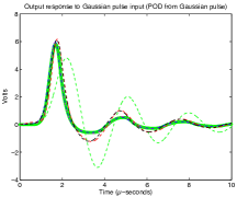
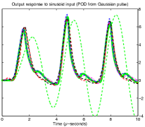
Fig. 5: Ladder Network: ROM responses to Gaussian pulse (left) and sinusoidal input (right).

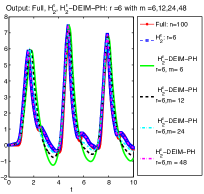
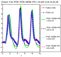
Fig. 6: Ladder Network: Outputs from $\mathcal{H}_{2}^{\varepsilon}$-ph reduced system (dimension $r=6$) and $\mathcal{H}_{2}^{\varepsilon}$-deim-phreduced systems ($\mathcal{H}_{2}^{\Large\varepsilon}$dimension $r=6$ with DIEM dimensions $m=6,12,14,48$)–similarly for the plot of pod-phand pod-deim-phreduced systems.

  

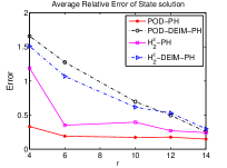
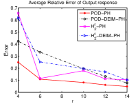
Fig. 7: Ladder Network: Average relative errors of the reduced systems constructed from pod-ph, pod-deim-ph, $\mathcal{H}_{2}^{\varepsilon}$-ph,  and $\mathcal{H}_{2}^{\varepsilon}$-deim-ph bases (with dimensions $r=2,4,....,18$ and deim dimension $m=3r$).

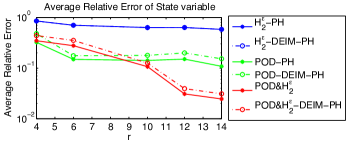
Fig. 8: Ladder Network: Average relative errors using the pod-ph, pod-deim-ph, $\mathcal{H}_{2}^{\varepsilon}$-ph, $\mathcal{H}_{2}^{\varepsilon}$-deim-ph, and the hybrid pod-$\mathcal{H}_{2}^{\varepsilon}$-ph and pod-$\mathcal{H}_{2}^{\varepsilon}$-deim-ph bases (with $r=2,4,....,18$ and deim dimension $m=3r$).

3.4.2 Toda Lattice

A Toda lattice model describes the motion of a chain of particles, each one connected to its nearest neighbors with ’exponential springs’. The equations of motion for the $N$-particle Toda lattice with such exponential interactions can be written in the form of a nonlinear port-Hamiltonian system as in (1) with

$$\mathbf{J}=\left[\begin{array}[]{cc}\rm{\bf 0}&\mathbf{I}\\ -\mathbf{I}&\rm{\bf 0}\end{array}\right]\in\mathbb{R}^{n\times n},~{}\mathbf{R}=\left[\begin{array}[]{cc}\rm{\bf 0}&\rm{\bf 0}\\ \rm{\bf 0}&\rm{diag}(\gamma_{1},\dots,\gamma_{N})\end{array}\right]\in\mathbb{R}^{n\times n},~{}\mathbf{B}=\left[\begin{array}[]{c}\rm{\bf 0}\\ \mathbf{e}_{1}\end{array}\right]\in\mathbb{R}^{n},$$

where $n=2N$ and

$$\mathbf{x}=\left[\begin{array}[]{c}\mathbf{q}\\ \mathbf{p}\end{array}\right]\in\mathbb{R}^{n},~{}~{}\mathbf{q}=[q_{1},\dots,q_{N}]^{T},~{}~{}\mathbf{p}=[p_{1},\dots,p_{N}]^{T}$$

with $q_{j}$ and $p_{j}$ being, respectively, the displacement of the $j$-th particle from its equilibrium position and the momentum of the $j$-th particle for $j=1,\dots,N$. In this example; we use $N=1000$ (i.e., the system dimension is $n=2000$), $\mathbf{x}_{0}={\bf 0}$, and $\gamma_{j}=0.1$, for $j=1,\dots,N$. The corresponding nonlinear Hamiltonian is given by

$$H(\mathbf{x})=H([\mathbf{q};\mathbf{p}])=\sum_{k=1}^{N}\frac{1}{2}p_{k}^{2}+\sum_{k=1}^{N-1}\exp(q_{k}-q_{k+1})+\exp(q_{N})-q_{1}-N.$$

The decomposition $H(\mathbf{x})=\mbox{$\frac{1}{2}$}\mathbf{x}^{T}\mathbf{Q}\mathbf{x}+h(\mathbf{x})$ is used with

$$\mathbf{Q}=\left[\begin{array}[]{cc}\mathbf{Q}_{0}&0\\ 0&\mathbf{I}\end{array}\right],\quad\mathbf{Q}_{0}=\left[\begin{array}[]{rrrrrrr}1&-1&0&\ldots&0&0\\ -1&2&-1&&&0\\ 0&-1&2&\ddots&&0\\ \vdots&&\ddots&\ddots&&&\\ &&&&-1&0\\ 0&&\ldots&-1&2&-1\\ 0&0&&0&-1&2\end{array}\right],$$

and $h(\mathbf{x})=\sum_{k=1}^{N-1}(q_{k}-q_{k+1})^{3}\varphi(q_{k}-q_{k+1})$ where $\varphi(z)=\frac{1}{2}\int_{0}^{1}\theta^{2}\,e^{(1-\theta)z}\,d\theta$. The system was excited with two different inputs: $u(t)=0.1$ and $u(t)=0.1\sin(t)$. Figure 9 shows that the outputs due to both inputs are accurately approximated by the outputs of the pod-ph and pod-deim-ph reduced systems. The average relative errors and the simulation times relative to the simulation time of the full model are illustrated in Figures 10 and 11. Notice that the accuracy of the pod-deim-ph reduced model captures that of the pod-ph model as the deim dimension $m$ increases. Note also that thepod-deim-ph reduced model cuts the simulation time by nearly $96\%$ while retaining accuracy.

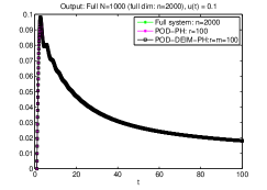
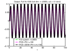
Fig. 9: Toda Lattice: The outputs from inputs $u(t)=0.1$ and $u(t)=0.1\sin(t)$.

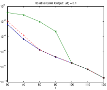
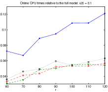
Fig. 10: Toda Lattice with input $u(t)=0.1$: Relative errors of the outputs and the online CPU times for pod-ph and pod-deim-ph reduced systems with POD basis dimension $r$ and DEIM dimension $m=r,m_{1},m_{2}$ where $m_{1}=r+$ ceil(r/3), $m_{2}=r+$ceil(2r/3); full-order system: $n=2000$.

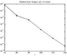
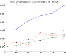
Fig. 11: Toda Lattice with input $u(t)=0.1\sin(t)$: Relative errors of the outputs and the online CPU times for pod-ph and pod-deim-ph  reduced systems with POD basis dimension $r$ and DEIM dimension $m=r,m_{1},m_{2}$ where $m_{1}=r+$ ceil(r/3), $m_{2}=r+$ceil(2r/3); full-order system: $n=2000$.

3.5 An a priori error bound for PH-preserving DEIM reduction

We derive error bounds for a deim-based reduced order model preserving PH-structure by estimating additional errors that occur by introducing the symmetrized-deim approximations into the structure-preserving reduction framework of §2. In particular, suppose that reduction bases, $\mathbf{V}_{r}$ and $\mathbf{W}_{r}$, have been chosen in some manner (e.g., as described as in §2.1, §2.2, or §2.3, say), and then are used to produce a reduced model that preserves the PH structure of the original system:

$$\begin{array}[]{ll}&\dot{\mathbf{x}}_{r}=(\mathbf{J}_{r}-\mathbf{R}_{r})\nabla_{\mathbf{x}_{r}}H_{r}(\mathbf{x}_{r})+\mathbf{B}_{r}\mathbf{u}(t)\\[5.69054pt] &\mathbf{y}_{r}\ =\ \mathbf{B}^{T}_{r}\nabla_{\mathbf{x}_{r}}H_{r}(\mathbf{x}_{r}).\end{array}$$ (29)

We then symmetrically ”sparsify” the nonlinear interactions in the Hamiltonian gradient evaluation and introduce a further deim-reduction as described in §3.3 and Algorithm 5 in order to produce:

$$\begin{array}[]{ll}&{\boldsymbol{\dot{\hat{x}}}}_{r}=(\mathbf{J}_{r}-\mathbf{R}_{r})\nabla_{{\boldsymbol{\hat{\mathit{x}}}}_{r}}\widehat{H}_{r}({\boldsymbol{\hat{\mathit{x}}}}_{r})+\mathbf{B}_{r}\mathbf{u}(t)\\[5.69054pt] &{\boldsymbol{\hat{\mathit{y}}}}_{r}\ =\ \mathbf{B}_{r}^{T}\nabla_{{\boldsymbol{\hat{\mathit{x}}}}_{r}}\widehat{H}_{r}({\boldsymbol{\hat{\mathit{x}}}}_{r})\end{array}$$ (30)

where $\mathbf{x}(0)={\boldsymbol{\hat{\mathit{x}}}}(0)$ and the deim Hamiltonian, $\widehat{H}$, has been defined in (26).

Theorem 6.

Let $\mathbf{x}_{r}(t)$ and $\mathbf{y}_{r}(t)$ be the state trajectory and output associated with the reduced port-Hamiltonian system (29). Suppose a deim basis of order $m$ has been chosen and used to define a deim projection $\mathbb{P}$ and deim Hamiltonian $\widehat{H}(\mathbf{x})$ as introduced in (26). Recalling the discussion of §3.2, suppose $\Omega\subset{\cal V}_{r}$ contains the trajectories $\mathbf{V}_{r}\mathbf{x}_{r}(t)$ and $\mathbb{P}^{T}\mathbf{V}_{r}\mathbf{x}_{r}$ and that $\varepsilon_{h}>0$ satisfies

$$\sup_{{\boldsymbol{\xi}}\in\Omega}\|\nabla_{\mathbf{x}}h({\boldsymbol{\xi}})-\mathbb{P}\nabla_{\mathbf{x}}h(\mathbb{P}^{T}{\boldsymbol{\xi}})\|_{\mathbf{Q}}\ \leq\ \varepsilon_{h}$$

Let ${\boldsymbol{\hat{\mathit{x}}}}_{r}(t)$ and ${\boldsymbol{\hat{\mathit{y}}}}_{r}(t)$ be the state trajectory and output associated with the deim-reduced port-Hamiltonian system (30).

Then with

$$\begin{array}[]{ccc}\alpha={\cal L}_{\mathbf{Q}}[\mathbf{G}]-\rho_{min},&\mathbf{G}({\boldsymbol{\xi}})=\mbox{\boldmath${\mathcal{P}}$}_{r}\mbox{\boldmath${\mathcal{A}}$}\mbox{\boldmath${\mathcal{P}}$}_{r}^{T}\mathbb{P}\nabla_{\mathbf{x}}h(\mathbb{P}^{T}{\boldsymbol{\xi}}),&\mbox{and}\quad\rho_{min}=\min\lambda(\mathbf{R}_{r})\\[5.69054pt] \beta=\|\mbox{\boldmath${\mathcal{P}}$}_{r}\mbox{\boldmath${\mathcal{A}}$}\mbox{\boldmath${\mathcal{P}}$}_{r}^{T}\|_{\mathbf{Q}},&\gamma=1+L_{\mathbf{Q}}[\mathbb{P}\,\nabla_{\mathbf{x}}h\circ\mathbb{P}^{T}],&\delta=\|\mathbf{B}\|\,\|\mbox{\boldmath${\mathcal{P}}$}_{r}\|\end{array}$$

we have, for $\alpha\neq 0$,

$$\begin{array}[]{c}\|\mathbf{x}_{r}(t)-{\boldsymbol{\hat{\mathit{x}}}}_{r}(t)\|\leq\frac{\beta}{\alpha}\left(e^{\alpha\,t}-1\right)\,\varepsilon_{h}\\[5.69054pt] \|\mathbf{y}_{r}(t)-{\boldsymbol{\hat{\mathit{y}}}}_{r}(t)\|\leq\delta\left(1+\frac{\beta\,\gamma}{\alpha}\left(e^{\alpha\,t}-1\right)\right)\,\varepsilon_{h},\end{array}$$ (31)

whereas for $\alpha=0$,

$$\begin{array}[]{c}\|\mathbf{x}_{r}(t)-{\boldsymbol{\hat{\mathit{x}}}}_{r}(t)\|\leq\beta\,t\,\varepsilon_{h}\\[5.69054pt] \|\mathbf{y}_{r}(t)-{\boldsymbol{\hat{\mathit{y}}}}_{r}(t)\|\leq\delta\left(1+\beta\,t\,\right)\,\varepsilon_{h}.\end{array}$$

Proof.

Let $\mathbf{e}_{r}(t):=\mathbf{x}_{r}(t)-{\boldsymbol{\hat{\mathit{x}}}}_{r}(t)$ be the difference between state trajectories generated by (29) and (30). Define $\mathbf{f}(\mathbf{x})=\nabla_{\mathbf{x}}h(\mathbf{x})$ and observe that

$$\frac{d}{dt}\|\mathbf{e}_{r}(t)\| =\left\langle\frac{\mathbf{e}_{r}(t)}{\|\mathbf{e}_{r}(t)\|},\dot{\mathbf{e}}_{r}(t)\right\rangle=\left\langle\frac{\mathbf{e}_{r}(t)}{\|\mathbf{e}_{r}(t)\|},\mathbf{A}_{r}\left[\nabla_{\mathbf{x}_{r}}H_{r}(\mathbf{x}_{r})-\nabla_{{\boldsymbol{\hat{\mathit{x}}}}_{r}}\widehat{H}_{r}({\boldsymbol{\hat{\mathit{x}}}}_{r})\right]\right\rangle$$

$$=\left\langle\frac{\mathbf{e}_{r}(t)}{\|\mathbf{e}_{r}(t)\|},\mathbf{A}_{r}\left[\mathbf{e}_{r}+\mathbf{V}_{r}^{T}\left(\nabla_{\mathbf{x}}h(\mathbf{V}_{r}\mathbf{x}_{r})-\mathbb{P}\,\nabla_{\mathbf{x}}h(\mathbb{P}^{T}\mathbf{V}_{r}{\boldsymbol{\hat{\mathit{x}}}}_{r})\right)\right]\right\rangle$$

We have

$$\left\langle\mathbf{e}_{r},\mathbf{A}_{r}\left[\mathbf{e}_{r}+\mathbf{V}_{r}^{T}\left(\nabla_{\mathbf{x}}h(\mathbf{V}_{r}\mathbf{x}_{r})-\mathbb{P}\,\nabla_{\mathbf{x}}h(\mathbb{P}^{T}\mathbf{V}_{r}{\boldsymbol{\hat{\mathit{x}}}}_{r})\right)\right]\right\rangle$$

$$\qquad=-\left\langle\mathbf{e}_{r},\mathbf{R}_{r}\mathbf{e}_{r}\right\rangle+\left\langle\mathbf{V}_{r}\mathbf{e}_{r},\,\mbox{\boldmath${\mathcal{P}}$}_{r}\mathbf{A}\mbox{\boldmath${\mathcal{P}}$}_{r}^{T}\left(\nabla_{\mathbf{x}}h(\mathbf{V}_{r}\mathbf{x}_{r})-\mathbb{P}\,\nabla_{\mathbf{x}}h(\mathbb{P}^{T}\mathbf{V}_{r}{\boldsymbol{\hat{\mathit{x}}}}_{r})\right)\right\rangle_{\mathbf{Q}}$$

$$\qquad=-\left\langle\mathbf{e}_{r},\mathbf{R}_{r}\mathbf{e}_{r}\right\rangle+\left\langle\mathbf{V}_{r}\mathbf{e}_{r},\,\mbox{\boldmath${\mathcal{P}}$}_{r}\mathbf{A}\mbox{\boldmath${\mathcal{P}}$}_{r}^{T}\left(\mathbb{P}\,\nabla_{\mathbf{x}}h(\mathbb{P}^{T}\mathbf{V}_{r}\mathbf{x}_{r})-\mathbb{P}\,\nabla_{\mathbf{x}}h(\mathbb{P}^{T}\mathbf{V}_{r}{\boldsymbol{\hat{\mathit{x}}}}_{r})\right)\right\rangle_{\mathbf{Q}}$$

$$\qquad\qquad+\left\langle\mathbf{V}_{r}\mathbf{e}_{r},\,\mbox{\boldmath${\mathcal{P}}$}_{r}\mathbf{A}\mbox{\boldmath${\mathcal{P}}$}_{r}^{T}\left(\nabla_{\mathbf{x}}h(\mathbf{V}_{r}\mathbf{x}_{r})-\mathbb{P}\,\nabla_{\mathbf{x}}h(\mathbb{P}^{T}\mathbf{V}_{r}\mathbf{x}_{r})\right)\right\rangle_{\mathbf{Q}}$$

$$\quad\leq-\rho_{min}\|\mathbf{e}_{r}\|^{2}+{\cal L}_{\mathbf{Q}}[\mathbf{G}]\,\|\mathbf{e}_{r}\|^{2}$$

$$\qquad\qquad+\|\mathbf{e}_{r}\|\ \|\mbox{\boldmath${\mathcal{P}}$}_{r}\mathbf{A}\mbox{\boldmath${\mathcal{P}}$}_{r}^{T}\|_{\mathbf{Q}}\,\|\nabla_{\mathbf{x}}h(\mathbf{V}_{r}\mathbf{x}_{r})-\mathbb{P}\,\nabla_{\mathbf{x}}h(\mathbb{P}^{T}\mathbf{V}_{r}\mathbf{x}_{r})\|_{\mathbf{Q}}$$

Thus,

$$\frac{d}{dt}\|\mathbf{e}_{r}(t)\|\leq \left({\cal L}_{\mathbf{Q}}[\mathbf{G}]-\rho_{min}\right)\,\|\mathbf{e}_{r}(t)\|$$

$$\qquad+\|\mbox{\boldmath${\mathcal{P}}$}_{r}\mathbf{A}\mbox{\boldmath${\mathcal{P}}$}_{r}^{T}\|_{\mathbf{Q}}\,\|\nabla_{\mathbf{x}}h(\mathbf{V}_{r}\mathbf{x}_{r}(t))-\mathbb{P}\,\nabla_{\mathbf{x}}h(\mathbb{P}^{T}\mathbf{V}_{r}\mathbf{x}_{r}(t))\|_{\mathbf{Q}}.$$

If $\alpha={\cal L}_{\mathbf{Q}}[\mathbf{G}]-\rho_{min}=0$ then trivially,

$$\|\mathbf{x}_{r}(t)-{\boldsymbol{\hat{\mathit{x}}}}_{r}(t)\|\leq\ \|\mbox{\boldmath${\mathcal{P}}$}_{r}\mathbf{A}\mbox{\boldmath${\mathcal{P}}$}_{r}^{T}\|_{\mathbf{Q}}\,\int_{0}^{t}\|\nabla_{\mathbf{x}}h(\mathbf{V}_{r}\mathbf{x}_{r}(\tau))-\mathbb{P}\,\nabla_{\mathbf{x}}h(\mathbb{P}^{T}\mathbf{V}_{r}\mathbf{x}_{r}(\tau))\|_{\mathbf{Q}}\,d\tau\leq\beta\,t\,\varepsilon_{h}.$$

If $\alpha\neq 0$ then by Gronwell’s inequality,

$$\|\mathbf{x}_{r}(t)-{\boldsymbol{\hat{\mathit{x}}}}_{r}(t)\| \leq\ \|\mbox{\boldmath${\mathcal{P}}$}_{r}\mathbf{A}\mbox{\boldmath${\mathcal{P}}$}_{r}^{T}\|_{\mathbf{Q}}\,\int_{0}^{t}e^{\alpha(t-\tau)}\,\|\nabla_{\mathbf{x}}h(\mathbf{V}_{r}\mathbf{x}_{r}(\tau))-\mathbb{P}\,\nabla_{\mathbf{x}}h(\mathbb{P}^{T}\mathbf{V}_{r}\mathbf{x}_{r}(\tau))\|_{\mathbf{Q}}\,d\tau$$

$$\leq\frac{\beta}{\alpha}\left(e^{\alpha\,t}-1\right)\,\varepsilon_{h}$$

This expression holds with a positive bound regardless of whether $\alpha>0$ or $\alpha<0$.

The resulting difference in output maps may be directly bounded:

$$\|\mathbf{y}_{r}-{\boldsymbol{\hat{\mathit{y}}}}_{r}\|\ =\ \|\mathbf{B}^{T}_{r}\left(\nabla_{\mathbf{x}_{r}}H_{r}(\mathbf{x}_{r})-\nabla_{{\boldsymbol{\hat{\mathit{x}}}}_{r}}\widehat{H}_{r}({\boldsymbol{\hat{\mathit{x}}}}_{r})\right)\|$$

$$=\ \|\mathbf{B}^{T}_{r}\left(\mathbf{x}_{r}-{\boldsymbol{\hat{\mathit{x}}}}_{r}+\mathbf{V}_{r}^{T}\left(\nabla_{\mathbf{x}}h(\mathbf{V}_{r}\mathbf{x}_{r})-\mathbb{P}\,\nabla_{\mathbf{x}}h(\mathbb{P}^{T}\mathbf{V}_{r}{\boldsymbol{\hat{\mathit{x}}}}_{r})\right)\right)\|$$

$$\leq\ \|\mathbf{B}^{T}_{r}\mathbf{e}_{r}\|+\|\mathbf{B}^{T}_{r}\mathbf{V}_{r}^{T}\left(\nabla_{\mathbf{x}}h(\mathbf{V}_{r}\mathbf{x}_{r})-\mathbb{P}\,\nabla_{\mathbf{x}}h(\mathbb{P}^{T}\mathbf{V}_{r}\mathbf{x}_{r})\right)\|$$

$$\ \qquad+\|\mathbf{B}^{T}_{r}\mathbf{V}_{r}^{T}\left(\mathbb{P}\,\nabla_{\mathbf{x}}h(\mathbb{P}^{T}\mathbf{V}_{r}\mathbf{x}_{r})-\mathbb{P}\,\nabla_{\mathbf{x}}h(\mathbb{P}^{T}\mathbf{V}_{r}{\boldsymbol{\hat{\mathit{x}}}}_{r})\right)\|$$

$$\leq\|\mathbf{B}\|\,\|\mbox{\boldmath${\mathcal{P}}$}_{r}\|\,\left(1+L_{\mathbf{Q}}[\mathbb{P}\,\nabla_{\mathbf{x}}h\circ\mathbb{P}^{T}]\right)\|\mathbf{x}_{r}(t)-{\boldsymbol{\hat{\mathit{x}}}}_{r}(t)\|+\|\mathbf{B}\|\,\|\mbox{\boldmath${\mathcal{P}}$}_{r}\|\,\varepsilon_{h},$$

which leads to the second conclusions respectively for $\alpha\neq 0$ and $\alpha=0$. ∎

4 Conclusions

We have introduced a structure-preserving projection-based model reduction framework for large-scale multi-input/multi-output nonlinear port-Hamiltonian systems. We constructed projection subspaces using three different approaches: pod, $\mathcal{H}_{2}$-based, and a hybrid pod-$\mathcal{H}_{2}$ based. We showed that for the same reduced order, the hybrid basis significantly outperforms the other two. We introduced a modification of deim within this framework to approximate the nonlinear part of the Hamiltonian gradient symmetrically. In all cases, the resulting reduced system preserves port-Hamiltonian structure, and thus retains the stability and passivity of the original system. We have derived the corresponding a priori error bounds of the state variables and outputs by using an application of generalized logarithmic norms for unbounded nonlinear operators. The effectiveness of the proposed approaches were shown on a nonlinear ladder network and a Toda lattice model.

References

- [1] P. Astrid, S. Weiland, K. Willcox, and T. Backx, Missing point estimation in models described by proper orthogonal decomposition, IEEE Transactions on Automatic Control, (2008), pp. 2237–2251.
- [2] M. Barrault, Y. Maday, N. Nguyen, and A. Patera, An “empirical interpolation” method: Application to efficient reduced-basis discretization of partial differential equations, Comptes Rendus Mathématique. Académie des Sciences. Paris, I (2004), pp. 339–667.
- [3] C. Beattie and S. Gugercin, Structure-preserving model reduction for nonlinear port-hamiltonian systems, in Decision and Control and European Control Conference (CDC-ECC), 2011 50th IEEE Conference on, Dec., pp. 6564–6569.
- [4] K. Carlberg, C. Farhat, J. Cortial, and D. Amsallem, The GNAT method for nonlinear model reduction: Effective implementation and application to computational fluid dynamics and turbulent flows, Journal of Computational Physics, 242 (2013), pp. 623–647.
- [5] K. Carlberg, R. Tuminaro, and P. Boggs, Preserving lagrangian structure in nonlinear model reduction with application to structural dynamics, SIAM Journal on Scientific Computing, 37 (2015), pp. B153–B184.
- [6] S. Chaturantabut and D. C. Sorensen, Nonlinear model reduction via discrete empirical interpolation, SIAM Journal on Scientific Computing, 32 (2010), pp. 2737–2764.
- [7] Z. Drmač and S. Gugercin, A new selection operator for the discrete empirical interpolation method–improved a priori error bound and extensions, SIAM Journal on Scientific Computing. Accepted to appear. Available as http://arxiv.org/abs/1505.00370, (2015).
- [8] V. Duindam, A. Macchelli, S. Stramigioli, and H. Bruyninckx, Modeling and control of complex physical systems, Springer, 2009.
- [9] R. Everson and L. Sirovich, The Karhunen-Loeve Procedure for Gappy Data, Journal of the Optical Society of America, 12 (1995), pp. 1657–1664.
- [10] K. Fujimoto and H. Kajiura, Balanced realization and model reduction of port-Hamiltonian systems, in American Control Conference, 2007, 2007, pp. 930–934.
- [11] K. Fujimoto and J. Scherpen, Balanced realization and model order reduction for nonlinear systems based on singular value analysis, SIAM Journal on Control and Optimization, 48 (2010), pp. 4591–4623.
- [12] S. Gugercin, A. C. Antoulas, and C. A. Beattie, model reduction for large-scale linear dynamical systems, SIAM J. Matrix Anal. Appl., 30 (2008), pp. 609–638.
- [13] S. Gugercin, R. Polyuga, C. Beattie, and A. van der Schaft, Interpolation-based Model Reduction for port-Hamiltonian Systems, in Proceedings of the Joint 48th IEEE Conference on Decision and Control and 28th Chinese Control Conference, Shanghai, PR China, 2009, pp. 5362–5369.
- [14] S. Gugercin, R. Polyuga, C. Beattie, and A. Van der Schaft, Structure-preserving tangential interpolation for model reduction of port-hamiltonian systems, Automatica, 48 (2012), pp. 1963–1974.
- [15] A. Hochman, B. Bond, and J. White, A stabilized discrete empirical interpolation method for model reduction of electrical, thermal, and microelectromechanical systems, in Design Automation Conference (DAC), 2011 48th ACM/EDAC/IEEE, June, pp. 540–545.
- [16] J. Lumley, The Structures of Inhomogeneous Turbulent Flow, Atmospheric Turbulence and Radio Wave Propagation, (1967), pp. 166–178.
- [17] B. Peherstorfer, D. Butnaru, K. Willcox, and H.-J. Bungartz, Localized discrete empirical interpolation method, SIAM Journal on Scientific Computing, 36 (2014), pp. A168–A192.
- [18] B. Peherstorfer and K. Willcox, Online adaptive model reduction for nonlinear systems via low-rank updates, SIAM Journal on Scientific Computing, 37 (2015), pp. A2123–A2150.
- [19] J. Phillips, Projection frameworks for model reduction of weakly nonlinear systems, in Proceedings of the 37th Annual Design Automation Conference, ACM, 2000, pp. 184–189.
- [20] R. V. Polyuga, Model Reduction of Port-Hamiltonian Systems, PhD thesis, University of Groningen, 2010.
- [21] R. V. Polyuga and A. van der Schaft, Structure preserving model reduction of port-Hamiltonian systems by moment matching at infinity, Automatica, 46 (2010), pp. 665–672.
- [22] , Structure preserving moment matching for port-Hamiltonian systems: Arnoldi and Lanczos, To appear in IEEE Transactions on Automatic Control, (2010).
- [23] M. Rewienski and J. White, A trajectory piecewise-linear approach to model order reduction and fast simulation of nonlinear circuits and micromachined devices, Computer-Aided Design of Integrated Circuits and Systems, IEEE Transactions on, 22 (2003), pp. 155–170.
- [24] J. Scherpen and A. van der Schaft, A structure preserving minimal representation of a nonlinear port-Hamiltonian system, in Decision and Control, 2008, 47th IEEE Conference on, 2008, pp. 4885–4890.
- [25] L. Sirovich, Turbulence and the dynamics of coherent structures. Part 1: Coherent structures, Quarterly of Applied Mathematics, 45 (1987), pp. 561–571.
- [26] G. Söderlind, The logarithmic norm. history and modern theory, BIT Numerical Mathematics, 46 (2006), pp. 631–652. 10.1007/s10543-006-0069-9.
- [27] D. B. Szyld, The Many Proofs of an Identity on the Norm of Oblique Projections, Numerical Algorithms, 42 (2006), pp. 309–323.
- [28] A. van der Schaft, Port-Hamiltonian systems: an introductory survey, in Proceedings of the International Congress of Mathematicians Vol. III, Madrid, M. Sanz-Sole, J. Soria, J. L. Varona, and J. Verdera, eds., Madrid, Spain, 2006, European Mathematical Society Publishing House (EMS Ph), pp. 1339–1365.
- [29] J. C. Willems, Dissipative dynamical systems part i: General theory, Archive for rational mechanics and analysis, 45 (1972), pp. 321–351.
- [30] H. Zwart and B. Jacob, Distributed-parameter port-hamiltonian systems, tech. rep., Technischer Bericht, Lehrstuhl für angewandte Mathematik, Universität Twente, Niederlande, 2009.