Abstract

We study SU$(N)$ Yang-Mills-Chern-Simons theory in the presence of defects that shift the Chern-Simons level from a holographic point of view by embedding the system in string theory. The model is a D3-D7 system in Type IIB string theory, whose gravity dual is given by the AdS soliton background with probe D7 branes attaching to the AdS boundary along the defects. We holographically renormalize the free energy of the defect system with sources, from which we obtain the correlation functions for certain operators naturally associated to these defects. We find interesting phase transitions when the separation of the defects as well as the temperature are varied. We also discuss some implications for the Fractional Quantum Hall Effect and for 2-dimensional QCD.

1 Introduction

Pure gauge theory in three dimensions has some distinguishing features when compared to its more familiar 4-dimensional cousin, which arise from two important differences: (1) the Yang-Mills (YM) coupling is a dimensionful quantity and determines the scale of confinement; and (2) in three dimensions it is possible to include a Chern-Simons (CS) term, inducing a gauge-invariant “topological mass” [1].

Pure Chern-Simons theory in particular has a wide range of interesting properties, and has seen numerous applications. Witten [2] showed that the expectation values of Wilson loop operators in $SU(2)$ CS theory reproduce the Jones polynomial knot invariants, leading to extensive development of its applications to knot theory. CS theory also has important applications in condensed matter theory, the most important perhaps being its use as an effective theory for the Fractional Quantum Hall Effect (FQHE). For example, $U(1)$ CS-theory at level $m$ gives the low energy effective theory of the $m^{\rm th}$ Laughlin state, which realizes the FQHE with filling fraction $\nu=1/m$ [3, 4] (for a review see, e.g., [5]). Another interesting aspect of CS theory is level-rank duality, the equivalence between the $U(N)$ CS theory at level $k$ and the $U(k)$ CS theory at level $N$ [6, 7, 8, 9]. This level-rank duality is related to Seiberg-like duality in 3-dimensional supersymmetric gauge theories [10, 11, 12, 13, 14, 15]. More recently, it has been generalized to non-supersymmetric theories with matter in the fundamental representation [16, 17, 18, 19, 20, 21, 22], providing rare examples of dualities in dynamical theories that can be established explicitly by exact calculations.

In this paper, we study the properties of 2-dimensional defects (domain walls) separating two phases at different CS levels in $SU(N)$ YM-CS theory using string theory and holography. While the CS term is not gauge-invariant in the presence of such level changing defects, the full quantum system is rendered consistent by the Callan-Harvey anomaly inflow mechanism [23]: the tree level gauge variation of the action is canceled by the chiral anomaly of chiral fermions that live on the defect.

There are several motivations for introducing such defects. One is to see how the defects behave under level-rank duality. Assuming that level-rank duality works locally, it predicts that the rank of the gauge group in the dual description jumps at the defect. We will give a geometric understanding of this phenomenon in terms of the brane configuration in the holographic model. A second motivation arises if we compactify one of the spatial directions to a circle, and introduce a defect anti-defect pair separated along the circle; the system then flows to 2-dimensional QCD at low energies. Two-dimensional QCD in the large $N$ limit is known to be solvable [25] and has rich structures, such as confinement and chiral symmetry breaking, similar to 4-dimensional QCD. We will discuss some interesting relations between 3-dimensional YM-CS theory and 2-dimensional QCD, which might shed some new light on the QCD physics. These defects are of interest in condensed matter physics as well, so it is of value to study them in the holographic context. As we will see, these defects generalize edges in the FQHE, and like FQH state edges, have gapless chiral excitations localized on them.

A string theory realization of the YM-CS system (without defects) was proposed in [26], where YM-CS dynamics is realized as the infrared behavior of a D3/D7 system. The 3-dimensional $SU(N)$ gauge theory with level $(-k)$ CS term is constructed by putting $N$ D3 branes compactified on an $S^{1}$ with SUSY-breaking boundary conditions and $k$ units of RR 1-form flux. The gravity dual is obtained by taking the near horizon limit of the background corresponding to the $N$ D3 branes (the AdS₅ soliton) in the presence of $k$ probe D7 branes wrapped on $S^{5}$. One nice feature of this construction is that its IR behavior explains the level-rank duality of CS theory. Furthermore, the fractionally quantized Hall conductivity was computed in both the gauge theory side and its gravity dual, and it was shown how the model could be used to compute the topological entanglement entropy. [27, 28, 29]

Our main goal is to show how to realize defects shifting the CS level from $(-k)$ to $(-k^{\prime})$ within this model, and to analyze the system in detail using holography. The defects are naturally realized geometrically by $|k-k^{\prime}|$ D7 branes peeling off the soliton tip to attach to the AdS boundary along the defect locus. Note that the gravity dual can be treated within the supergravity approximation when $N$ and the ’t Hooft coupling $\lambda_{\rm 3d}=g_{\rm 3d}^{2}N$ are large. Therefore, we are dealing with large $N$ strongly coupled regime of the 3-dimensional gauge theory.

Although the direct relevance of the large $N$ gauge theories to condensed matter systems is perhaps questionable, non-Abelian CS theory does have known applications to condensed matter theory. In the FQH state with filling fraction $\nu=\frac{1}{2}$, for example, the effective theory of the fermionic Moore-Read Pfaffian state can be derived by flux attachment from the $SU(2)_{2}$ CS theory describing the bosonic Pfaffian state at $\nu=1$ [30]. The (non-abelian) edge states of the non-Abelian CS theory are also known to play an important role in the context of FQHE, being the edge excitations which carry the topologically protected and quantized Hall response [33, 34, 35]. In fact, the derivation of the bulk effective $SU(2)_{2}$ CS action in [30] started from the observation that the edge theory of the bosonic Pfaffian state at $\nu=1$ is a $SU(2)_{2}$ Kac-Moody algebra.

The contents of this paper can be summarized as follows. We begin in section 2 by introducing 3-dimensional $SU(N)$ YM-CS field theory and its level-changing defects, followed by its realization by probe branes in section 3. Section 4 analyses the probe D7($\overline{\rm D7}$) branes on the gravity side and gives general solutions for the transverse scalar and the worldvolume gauge fields. In section 5, we perform the holographic renormalization of the on-shell D7-brane action, and use the renormalized action to compute holographic correlation functions of defect operators. Section 6 uses these results to evaluate the free energy of the D7-brane configuration, revealing a phase transition in the correlation functions across defects pairs as a function of defect separation; studies in greater detail the question of confinement in YM-CS from the point of view of the gravity dual; and computes the chiral condensate that forms between the chiral fermions living on adjacent defect/anti-defect pairs. In section 7, we generalize our considerations to finite temperature by replacing the AdS soliton with the AdS black hole, and study the effects of finite temperature on the phase transitions of the cross-defect correlators. Finally in section 8, we summarize our results and discuss some of the implications and the outlook. In particular, we point out an interesting relation between the FQHE and 2-dimensional QCD, and discuss possible applications of our model to FQH physics. Our notational conventions are summarized in Appendix A, and details of the solutions of the D7-brane equations of motion can be found in Appendix B.

2 Yang-Mills-Chern-Simons theory and its level-changing defects

In this section, we consider 3-dimensional $SU(N)$ YM-CS theory defined on a flat spacetime parametrized by $x^{\mu}$ ($\mu=0,1,2$). We study this theory in the presence of 2-dimensional defects (domain walls) at which the CS level changes. To simplify things, we consider only defects extended along the $x^{\pm}\equiv(x^{0}\pm x^{1})/2$ directions at fixed values of $y\equiv x^{2}$ so that the 2-dimensional Lorentz symmetry is preserved.

As a first example, let us consider a defect placed at $y=0$, as depicted in the left panel of Fig. 1. The level of the CS term is set to be $(-k)$ and $(-k^{\prime})$ for the regions $y<0$ and $y>0$, respectively. We assume that $k$ and $k^{\prime}$ are integers satisfying $k>k^{\prime}$. The Lagrangian for the $SU(N)$ gauge field $A=A_{\mu}dx^{\mu}$ is

$$S_{A}=-\frac{1}{4g_{\rm 3d}^{2}}\int d^{3}x\,{\rm Tr}(F^{\mu\nu}F_{\mu\nu})-\frac{k}{4\pi}\int_{y<0}\omega_{3}(A)-\frac{k^{\prime}}{4\pi}\int_{y>0}\omega_{3}(A)\ ,$$ (2.1)

where $\omega_{3}(A)$ is the Chern-Simons 3-form

$$\omega_{3}(A)\equiv\operatorname{\mathrm{Tr}}\left(A\wedge dA-\frac{2i}{3}A\wedge A\wedge A\right)\ .$$ (2.2)

Note that the CS 3-form transforms as

$$\delta_{\alpha}\omega_{3}(A)=d{\rm Tr}(\alpha\,dA)\ ,$$ (2.3)

under the infinitesimal gauge transformation $\delta_{\alpha}A=d\alpha-i[A,\alpha]$, and the action (2.1) transforms as

$$\delta_{\alpha}S_{A}=\frac{k^{\prime}-k}{4\pi}\int_{y=0}\operatorname{\mathrm{Tr}}({\alpha\,dA})\ .$$ (2.4)

Here, we have assumed that the gauge field is continuous at $y=0$, and dropped boundary terms at infinity not relevant for our discussion. In order to have a gauge invariant action, we put $(k-k^{\prime})$ negative chirality Weyl fermions $\psi_{-}^{i}$ ($i=1,2,\cdots,k-k^{\prime}$), which transform as the fundamental representation of the gauge group $SU(N)$, on the 2-dimensional defect at $y=0$. The subscript “$-$” of $\psi_{-}^{i}$ indicates the chirality of the fermion. The action for the chiral fermions is

$$S_{\psi}=\int_{y=0}d^{2}x\,\psi_{-i}^{\dagger}(i\partial_{+}+A_{+})\psi_{-}^{i}\ ,$$ (2.5)

where $\partial_{\pm}\equiv\partial_{0}\pm\partial_{1}$ and $A_{\pm}\equiv A_{0}\pm A_{1}$. The gauge anomaly induced by the chiral fermion precisely cancels the anomalous gauge transformation due to the CS term (2.4), and the whole system is gauge invariant.

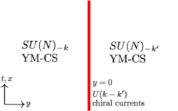
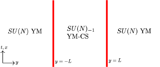
Fig. 1: Left: A (1+1)-dimensional defect in (2+1)-dimensional $SU(N)$ YM-CS theory. Chiral fermions on the defect induce the jump in the CS level when crossing the defect, and give rise to chiral $U(k-k^{\prime})$ global currents. Right: A more complicated configuration in which a YM-CS vacuum with nontrivial level can exist between vacua of pure YM theory if the fermions on both defects are equal in number but opposite in chirality.

In the following sections, we consider operators inserted on the defects. An important example for the defect operators is the current operator associated to the $U(k-k^{\prime})$ global symmetry, which acts on the chiral fermions on the defect, defined as

$$J^{a+}\equiv\psi_{-j}^{\dagger}(T^{a})^{j}_{~{}i}\psi_{-}^{i}\ ,$$ (2.6)

where $T^{a}$ are the generators of the $U(k-k^{\prime})$ symmetry. When the external gauge field ${\cal A}_{+}$ associated to the $U(k-k^{\prime})$ symmetry is introduced in the action (2.5), it naturally couples with the current operator as

$$\int_{y=0}d^{2}x\,{\cal A}^{a}_{+}J^{a+}\ .$$ (2.7)

As with any gauge field, coupling an external gauge field to 2-dimensional chiral fermions gives rise to a chiral anomaly. From the point of view of the external $U(k-k^{\prime})$ symmetry there are $N$ chiral fermions, and as a result the gauge variation $\delta{\cal A}^{a}_{+}=D_{+}\Lambda^{a}$ of the effective action $S({\cal A})$ takes the form

$$\delta_{\Lambda}S({\cal A})=\frac{N}{4\pi}\int d^{2}x\,\Lambda^{a}\partial_{-}{\cal A}_{+}^{a}\ .$$ (2.8)

From $\delta W[{\cal A}]=\int d^{2}x\,J^{a\mu}(x)\delta{\cal A}^{a}_{\mu}(x)$ and the relation $J_{-}=-2J^{+}$ we obtain the anomalous current conservation equation

$$\langle D_{+}J_{-}\rangle=\frac{N}{2\pi}\partial_{-}{\cal A}_{+}\ .$$ (2.9)

Another example is the operator associated with the displacement of the defect. If we put the defect at $y=\epsilon$ with $|\epsilon|\ll 1$, the chiral fermions couple with the gauge field evaluated at $y=\epsilon$ and hence the action (2.5) is modified as

$$S_{\psi} \simeq \int_{y=0}d^{2}x\left(\psi_{-i}^{\dagger}(i\partial_{+}+A_{+})\psi_{-}^{i}+\epsilon\,{\cal O}_{y}\right)\ ,$$ (2.10)

where

$${\cal O}_{y}\equiv\psi_{-i}^{\dagger}F_{y+}\psi_{-}^{i}\ ,$$ (2.11)

and $F_{y+}=\partial_{y}A_{+}-\partial_{+}A_{y}-i[A_{y},A_{+}]$. We will also consider a third operator that does not have such a straightforward geometric interpretation from the point of view of the field theory, the dimension 5 operator

$${\cal O}_{+}\equiv\psi_{-i}^{\dagger}F_{+y}F_{+y}\psi^{i}_{-}\ .$$ (2.12)

When $k<k^{\prime}$ then, as the coefficient of (2.4) has the opposite sign, we should introduce $(k^{\prime}-k)$ chiral fermions with positive chirality $\psi_{+}^{i}$ ($i=1,2,\cdots,k^{\prime}-k$) on the defect. Then, the action for the fermions with the source terms is

$$S_{\psi}=\int_{y=0}d^{2}x\,\left(\psi_{+i}^{\dagger}(i\partial_{-}+A_{-})\psi_{+}^{i}+{\cal A}_{-}^{a}J^{a-}+\epsilon{\cal O}^{\prime}_{y}\right)\ ,$$ (2.13)

where

$$J^{a-}\equiv\psi_{+j}^{\dagger}(T^{a})^{j}_{~{}i}\psi_{+}^{i}$$ (2.14)

is the current operator associated with the $U(k^{\prime}-k)$ symmetry and ${\cal O}^{\prime}_{y}$ is defined as

$${\cal O}^{\prime}_{y}\equiv\psi_{+i}^{\dagger}F_{y-}\psi_{+}^{i}\ .$$ (2.15)

The generalization to more complicated configurations is straightforward. In sections 4–7, we will mainly consider the case with two defects at $y=-L$ and $y=L$, which change the level of the CS term from $0$ to $-1$ at $y=-L$ and $-1$ to $0$ at $y=L$ along the $y$ axis. Such a configuration is depicted in the right panel of Fig. 1. The action for the gauge field is

$$S_{A}=-\frac{1}{4g_{\rm 3d}^{2}}\int d^{3}x\,{\rm Tr}(F^{\mu\nu}F_{\mu\nu})-\frac{1}{4\pi}\int_{-L<y<L}\omega_{3}(A)\ .$$ (2.16)

In this case, we put positive and negative chirality fermions at $y=-L$ and $y=L$, respectively. In the region with $|y|>L$, the theory is pure YM theory without CS term.

YM theory in 3-dimensions is known to have a mass gap due to confinement and the Wilson loop exhibits area law behavior. Pure CS theory on the other hand is a topological theory, so that the expectation value of Wilson lines depends only on topology and is independent of separation. It is a non-trivial question which behavior arises in the region between the two defects: the system should be gapped, as the CS term gives the gauge field a mass at tree level, but if the gap is sufficiently smaller than the confinement scale, the confining behavior may take over. (See, e.g., [36, 37] for a discussion of related issues.) We address the question of confinement in our system in section 6.3.

3 Brane configuration

We now turn to the realization of 3-dimensional YM-CS theory with level-changing defects by the infrared behavior of a brane configuration in string theory.

Consider Type IIB string theory compactified on an $S^{1}$ of radius $M_{\rm KK}^{-1}$ and $N$ D3 branes wrapped on it. The D3 brane is extended along $x^{0}$, $x^{1}$, $x^{2}\equiv y$ and $x^{3}\equiv\tau$ directions, where $\tau$ parametrizes the $S^{1}$ direction. Following [38], we impose an anti-periodic boundary condition on all the fermions along the $S^{1}$. This SUSY-breaking boundary condition gives all fermion modes a tree level mass of order $M_{\mathrm{KK}}$. Quantum corrections then induce masses in the scalar fields, lifting them from the infrared spectrum. The resulting theory is thus expected to flow to 3-dimensional pure $SU(N)$ YM theory at low energies. The gauge coupling $g_{\rm 3d}$ for the 3-dimensional YM theory is identified with

$$g_{\rm 3d}^{2}=g_{s}M_{\rm KK}\ ,$$ (3.1)

where $g_{s}$ is the string coupling.

Note that we can safely take the limit $l_{s}\rightarrow 0$, where $l_{s}$ is the string length, so that all the stringy excited states become infinitely heavy and the couplings to closed strings vanish. To be precise, the resulting theory is not exactly pure 3-dimensional YM theory, but ${\cal N}=4$ supersymmetric YM theory compactified on the $S^{1}$ with SUSY-breaking boundary conditions. The 3-dimensional pure YM theory is realized as the massless sector of this configuration, but there are infinitely many massive Kaluza-Klein (KK) modes associated to the $S^{1}$. In principle, in order to make the KK modes infinitely heavy, we should take the limit $M_{\rm KK}\rightarrow\infty$ with $\lambda_{\rm 3d}\equiv g_{\rm 3d}^{2}N$ kept finite by tuning $g_{s}\rightarrow 0$. However, in the following sections, we study the holographic description within the supergravity approximation, which can be trusted only when $N\gg 1$ and $\lambda_{\rm 3d}\gg M_{\rm KK}$. Therefore, it is not possible to decouple the Kaluza-Klein modes in the parameter region we are going to consider. For this reason, we will keep $M_{\rm KK}$ finite, and mainly consider the low energy behavior of the theory. We hope that the KK modes will not alter the qualitative behavior at low energies.

The CS term is obtained by introducing non-zero RR flux $dC_{0}$, where $C_{0}$ is the RR 0-from field, along the $S^{1}$.[26] Recall that the CS term of the D3-brane action has the following term when $dC_{0}$ is non-trivial:

$$S_{\rm CS}^{\rm D3}=-\frac{1}{8\pi^{2}}\int_{R^{3}\times S^{1}}dC_{0}\wedge\omega_{3}(A)\ .$$ (3.2)

Therefore, when we have

$$\int_{S^{1}}dC_{0}=2\pi k\ ,$$ (3.3)

(3.2) gives the CS term at level $(-k)$ and hence we obtain the brane configuration corresponding to the 3-dimensional $SU(N)$ YM-CS theory at low energies.

In order to introduce 2-dimensional defects with chiral fermions on them, we put D7 branes extended along $x^{0}$, $x^{1}$, $x^{4},\cdots,x^{9}$ directions, as considered in [44, 45, 46] for the supersymmetric case. When $n$ D7 branes are placed at $y=\tau=0$, the 3-7 strings (open strings stretched between D3 branes and D7 branes) give $n$ flavors of chiral fermions as the massless modes. In addition, since the D7 branes are magnetically charged under RR 0-form field $C_{0}$, we have the relation

$$\int_{S^{1}_{-}}dC_{0}-\int_{S^{1}_{+}}dC_{0}=2\pi n\ ,$$ (3.4)

where $S^{1}_{+}$ and $S^{1}_{-}$ are the $S^{1}$ in the $\tau$ direction with $y>0$ and $y<0$, respectively. Choosing $C_{0}$ to satisfy

$$\int_{S^{1}_{+}}dC_{0}=2\pi k^{\prime}\ ,~{}~{}\int_{S^{1}_{-}}dC_{0}=2\pi k\ ,$$ (3.5)

with $n=k-k^{\prime}$, the CS term (3.2) becomes

$$S_{\rm CS}^{\rm D3}=-\frac{k}{4\pi}\int_{y<0}\omega_{3}(A)-\frac{k^{\prime}}{4\pi}\int_{y>0}\omega_{3}(A)\ ,$$ (3.6)

which agrees with the CS term in (2.1). In this way, the first example in section 2 is obtained by putting $(k-k^{\prime})$ D7 branes at $y=\tau=0$.

Similarly, the brane configuration that realizes the theory in (2.16) is given by placing a D7 brane and a $\overline{\rm D7}$ brane at $y=L$ and $y=-L$, respectively. It is known that the chirality of the massless fermion in the spectrum of the 3-$\overline{7}$ strings is opposite to that of the 3-7 strings, as required by the anomaly cancellation discussed in section 2. This configuration is a close analogue to the D4-D8-$\overline{\rm D8}$ system used in [47] to obtain a holographic description of QCD. In fact, if we place $N_{f}$ D7 branes at $(y,\tau)=(0,0)$ and $N_{f}$ $\overline{\rm D7}$ branes at $(y,\tau)=(0,\pi M_{\rm KK}^{-1})$, and T-dualize along the $y$ direction, we obtain the D2-D8-$\overline{\rm D8}$ system considered in [48, 49], which is the 2-dimensional version of the holographic QCD.

One may question the stability of this brane configuration. At the least we must make sure that the separation between the D7 brane and the $\overline{\rm D7}$ brane is larger than the string length scale $l_{s}$ so that there is no tachyonic mode in the spectrum of the open strings connecting the D7 brane and the $\overline{\rm D7}$ brane. In addition, because the D7 brane and the $\overline{\rm D7}$ brane are attracted to each other by closed string exchange, the asymptotic behavior of the branes may need to be modified to pull the D7 brane and $\overline{\rm D7}$ branes apart at infinity so as to balance the force. We will not try to investigate this issue in this paper. In the following sections, we will only consider the near horizon limit of the D3-brane background and assume that we can work in the probe approximation [50], in which the backreaction due to the D7 branes is neglected, with $N$ being much larger than the number of D7 branes. At least in this limit, it is possible to show that there are no tachyonic modes in the fluctuations of the D7 brane in the holographic description.

4 Holographic description

4.1 Background geometry

As mentioned in the previous section, we treat D7 branes as probe branes embedded in the near horizon geometry corresponding to the D3-brane background. The background corresponding to the D3 brane considered in section 3 is called the AdS soliton background. The metric as well as the configuration of the other fields for this background is explicitly known.[38] The metric is given by

$$ds^{2}=\frac{u^{2}}{R^{2}}\left(\eta_{\mu\nu}dx^{\mu}dx^{\nu}+f(u)d\tau^{2}\right)+\frac{R^{2}}{u^{2}}\frac{du^{2}}{f(u)}+R^{2}d\Omega_{5}^{2}\ ,$$ (4.1)

where $\eta_{\mu\nu}={\rm diag}(-1,1,1)$ $(\mu,\nu=0,1,2)$ is the 3-dimensional Minkowski metric, $d\Omega_{5}^{2}$ is the line element of the unit $S^{5}$, and

$$f(u)\equiv 1-\frac{u_{0}^{4}}{u^{4}}\ .$$ (4.2)

We also use the coordinates $x^{\pm}\equiv\frac{1}{2}(x^{0}\pm x^{1})$ and $y\equiv x^{2}$ as we did in the previous section. Since $f(u)$ should be positive, the radial coordinate $u$ is restricted as $u\geq u_{0}$. The $\tau$ direction is compactified to a circle of radius $M_{\rm KK}^{-1}$ by the identification

$$\tau\sim\tau+2\pi M_{\rm KK}^{-1}\ .$$ (4.3)

To avoid a conical singularity at $u=u_{0}$, $M_{\rm KK}$ must be related to $u_{0}$ and $R$ by

$$M_{\rm KK}=\frac{2u_{0}}{R^{2}}\ .$$ (4.4)

The dilaton field $\phi$ is constant and it is related to the string coupling $g_{s}$ as $g_{s}=e^{\phi}$. The parameter $R$ in the metric (4.1) is related to the string length $l_{s}=\sqrt{\alpha^{\prime}}$ and the number of D3 branes $N$ as

$$R^{4}=4\pi g_{s}Nl_{s}^{4}\ .$$ (4.5)

In addition, the RR 5-form field strength $F_{5}$ satisfies

$$\int_{S^{5}}F_{5}=2\pi N\ .$$ (4.6)

4.2 Probe D7 brane

In order to find a consistent D7-brane configuration, we have to solve the equations of motion for the fields on the D7-brane world-volume. The D7 branes corresponding to the defects considered in the previous section are extended along $x^{M}=(x^{0},x^{1},u)$ directions and wrapped on the $S^{5}$. However, since the coordinate $u$ is bounded from below, it has to bend in one of the boundary directions. Let us start with a single D7 brane embedded in the background. We parametrize the D7-brane world-volume using $x^{M}$ and the coordinates of the $S^{5}$. For simplicity, we only turn on 3-dimensional components $a_{M}$ ($M=0,1,u$) of the $U(1)$ gauge field on the D7 brane and consider the configurations that are uniform along the $S^{5}$ directions. The position of the D7 brane in the $(y,\tau)$ space is given by the functions $y=y(x^{M})$ and $\tau=\tau(x^{M})$, which are treated as scalar fields on the D7 brane. The effective action is

$$S^{\rm D7}=S^{\rm D7}_{\rm DBI}+S^{\rm D7}_{\rm CS}$$ (4.7)

with

$$S^{\rm D7}_{\rm DBI} = -\frac{1}{(2\pi)^{7}l_{s}^{8}g_{s}}\int dx^{0}dx^{1}du\,vol(S^{5})R^{5}\sqrt{-\det\left(g_{MN}+(2\pi\alpha^{\prime})f_{MN}\right)}\ ,$$ (4.8)

$$S^{\rm D7}_{\rm CS} = \frac{1}{8\pi^{2}}\int F_{5}\wedge a\wedge da\ ,$$ (4.9)

where $vol(S^{5})$ is the volume form of the unit $S^{5}$, $g_{MN}$ is the induced metric, $a=a_{M}dx^{M}$ is the gauge field on the D7 brane and $f_{MN}\equiv\partial_{M}a_{N}-\partial_{N}a_{M}$ is its field strength. The induced metric can be written explicitly as

$$g_{MN}=G_{MN}+G_{ij}\partial_{M}y^{i}\partial_{N}y^{j}\ ,$$ (4.10)

where $y^{i}=(y,\tau)$ are the embedding functions and $(G_{MN},G_{ij})$ are part of the background metric read from (4.1), whose non-zero components are given as

$$G_{\mu\nu}=\frac{u^{2}}{R^{2}}\eta_{\mu\nu}\ ,~{}~{}G_{uu}=\frac{R^{2}}{u^{2}}\frac{1}{f(u)}\ ,~{}~{}G_{yy}=\frac{u^{2}}{R^{2}}\ ,~{}~{}G_{\tau\tau}=\frac{u^{2}}{R^{2}}f(u)\ .$$ (4.11)

Integrating over the $S^{5}$, the action is reduced to the 3-dimensional DBI-CS action:

$$S^{\rm D7}_{\rm DBI} = -T_{\rm 3d}\int dx^{0}dx^{1}du\sqrt{-{\cal G}}\ ,$$ (4.12)

$$S^{\rm D7}_{\rm CS} = \frac{N}{4\pi}\int a\wedge da=\frac{N}{8\pi}\int dx^{0}dx^{1}du\left(a_{-}f_{+u}-a_{+}f_{-u}-a_{u}f_{+-}\right)\ ,$$ (4.13)

where the effective 3d tension is given by

$$T_{\rm 3d} =\frac{RN}{8\pi(2\pi\alpha^{\prime})^{2}}\ ,$$ (4.14)

and ${\cal G}$ is defined as

$${\cal G} =\det({\cal G}_{MN})\ ,$$ (4.15)

where

$${\cal G}_{MN} =g_{MN}+(2\pi\alpha^{\prime})f_{MN}\ .$$ (4.16)

Here we have used (4.5) and (4.6). Note that the level of the CS term (4.13) is $N$, which we take to be positive.

The equations of motion for the transverse embedding coordinates $y^{i}=(y,\tau)$ and the gauge field $a_{M}$ take the form

$$\partial_{M}\left(\sqrt{-{\cal G}}G_{ij}{\cal G}^{MN}_{S}\partial_{N}y^{j}\right) =0\ ,$$ (4.17)

$$(2\pi\alpha^{\prime})T_{\rm 3d}\partial_{M}\left(\sqrt{-{\cal G}}{\cal G}_{A}^{MN}\right) =\frac{N}{4\pi}\epsilon^{NPQ}f_{PQ}\ .$$ (4.18)

Here ${\cal G}_{S}^{MN}$ and ${\cal G}_{A}^{MN}$ are defined as

$${\cal G}_{\rm S}^{MN} =\frac{1}{2}({\cal G}^{MN}+{\cal G}^{NM})\ ,$$ (4.19)

$${\cal G}_{\rm A}^{MN} =\frac{1}{2}({\cal G}^{MN}-{\cal G}^{NM})\ ,$$ (4.20)

which are respectively the symmetric and antisymmetric parts of the inverse matrix ${\cal G}^{MN}$ of ${\cal G}_{MN}$, i.e. ${\cal G}^{MN}{\cal G}_{NP}=\delta^{M}_{P}$. (See Appendix B.1 for more details.) In Appendix B.2, we summarize the solutions of these equations in the case that $y^{i}$ and $f_{MN}$ depend only on $u$. If we further assume that the gauge field $a_{M}$ depends only on $u$, the most general solution is

$$y(u) = y_{0}+c_{y}\int^{u}_{u_{\rm min}}du^{\prime}\frac{R^{5}}{F(u^{\prime})}\ ,$$ (4.21)

$$\tau(u) = \tau_{0}+c_{\tau}\int_{u_{\rm min}}^{u}du^{\prime}\frac{R^{5}}{f(u^{\prime})F(u^{\prime})}\ ,$$ (4.22)

$$a_{\pm}(u) = a_{\pm}^{(0)}\pm\frac{c_{\pm}}{8\pi\alpha^{\prime}}\exp\left(\mp 4\int_{u_{\rm min}}^{u}du^{\prime}\frac{u^{\prime 4}}{F(u^{\prime})}\right)\ ,$$ (4.23)

where $y_{0}$, $c_{y}$, $\tau_{0}$, $c_{\tau}$, $a_{\pm}^{(0)}$, $c_{\pm}$ and $u_{\rm min}$ are constants, and

$$F(u)\equiv\sqrt{u^{4}f(u)\left(u^{6}+u^{4}c_{+}c_{-}-R^{6}c_{y}^{2}-\frac{R^{6}c_{\tau}^{2}}{f(u)}\right)}\ .$$ (4.24)

To see what the solution looks like, consider the case with $\tau_{0}=c_{\tau}=a_{\pm}^{(0)}=c_{\pm}=0$ and $c_{y}>0$. Then, (4.21) becomes

$$y(u)=y_{0}+R^{2}u_{*}^{3}\int_{u_{\rm min}}^{u}\frac{du^{\prime}}{\sqrt{(u^{\prime 4}-u_{0}^{4})(u^{\prime 6}-u_{*}^{6})}}\ ,$$ (4.25)

where $u_{*}\equiv Rc_{y}^{1/3}$.

Naïvely, for a given choice of asymptotic boundary conditions on $y(u)$ as $u\to\infty$ there are two distinct branches of solutions, one with $u_{*}\geq u_{0}$ and the other with $u_{*}<u_{0}$. However, the second branch corresponds to a D7 brane whose two ends asymptotically approach opposite sides of the $\tau$ circle. To better understand this solution, define coordinates $(\rho,\theta)$ on the $(u,\tau)$ plane by the identifications

$$\rho^{2}=\frac{R^{2}u^{2}}{4u_{0}^{2}}f(u)\ ,\qquad\theta=\frac{2u_{0}}{R^{2}}\tau\ .$$ (4.26)

Note that $\theta$ has periodicity $2\pi$. The 5-dimensional metric takes on the form

$$ds^{2}_{5}=\frac{u^{2}(\rho)}{R^{2}}\eta_{\mu\nu}dx^{\mu}dx^{\nu}+\frac{4u_{0}^{2}/u^{2}(\rho)}{\left(1+u_{0}^{4}/u^{4}(\rho)\right)^{2}}\,d\rho^{2}+\rho^{2}\,d\theta^{2}\ .$$ (4.27)

We further introduce coordinates $(v,w)$ by

$$v=\rho\,\cos\theta\ ,\qquad w=\rho\,\sin\theta\ ,$$ (4.28)

in which the asymptotic region corresponds to $\rho^{2}=v^{2}+w^{2}\to\infty$. The solutions we consider have $\tau=0$, which in the new coordinates is $w=0$. We thus wish to solve for $y$ as a function of $v$. The differential relation now becomes

$$\frac{dy}{dv}=\frac{2Ru_{*}^{3}u_{0}}{u^{2}(v)(1+u_{0}^{4}/u^{4}(v))\sqrt{u^{6}(v)-u_{*}^{6}}}\ .$$ (4.29)

In the case $u_{*}<u_{0}$, the resulting brane profile $v(y)$ does not have a turning point. Instead, the solutions behave as $v(y)\to\pm\infty$ as $y\to\pm\infty$. Referring to our original coordinate system, we see that $w=0$, $v<0$ corresponds to the angular position $\theta=\pi$. Thus the branch $u_{*}<u_{0}$ corresponds to a defect with $\theta\to 0$ as $v\to\infty$, and $\theta\to\pi$ as $v\to-\infty$.

We will therefore focus on the case $u_{*}\geq u_{0}$. It is convenient to choose $u_{\rm min}=u_{*}$ and $y_{0}=0$. This solution makes sense for $u\geq u_{*}$ and terminates at $u=u_{*}$. Actually, $u=u_{*}$ is a turning point and the solution is smoothly connected to the solution obtained by flipping the sign of $c_{y}$ as

$$y(u)=\pm R^{2}u_{*}^{3}\int_{u_{*}}^{u}\frac{du^{\prime}}{\sqrt{(u^{\prime 4}-u_{0}^{4})(u^{\prime 6}-u_{*}^{6})}}\ .$$ (4.30)

The solution is U-shaped as depicted in Fig. 2.

Fig. 2: A plot of the solution (4.30) with $u_{0}=R=1$ and $u_{*}=1.1$.

The asymptotic value of $y$ is given by $y({u=\infty})=\pm L$ with

$$L\equiv\lim_{u\rightarrow\infty}|y(u)|=R^{2}u_{*}^{3}\int_{u_{*}}^{\infty}\frac{du}{\sqrt{(u^{4}-u_{0}^{4})(u^{6}-u_{*}^{6})}}\ .$$ (4.31)

It is often convenient to use a coordinate that can smoothly parametrize the D7-brane world-volume around $u=u_{*}$. One way to do this is to introduce a coordinate $z$ related to $u$ by

$$u^{2}=u_{*}^{2}(1+z^{2})\ .$$ (4.32)

Then, (4.30) can be written as

$$y(z)=R^{2}u_{*}\int_{0}^{z}\frac{dz}{\sqrt{(u_{*}^{4}(1+z^{2})^{2}-u_{0}^{4})(1+z^{2})(3+3z^{2}+z^{4})}}\ ,$$ (4.33)

which is valid for $-\infty<z<\infty$.

The configuration given by the solution (4.30) corresponds to the case with a D7 brane and $\overline{\rm D7}$ brane placed at $y=L$ and $y=-L$, respectively, considered in section 3. As explained around (3.2), the CS level for the $SU(N)$ YM-CS theory is given by the integration of the RR 1-form field strength $dC_{0}$ along the $S^{1}$ parametrized by $\tau$. In the holographic description, it corresponds to minus the number of D7 branes penetrating the $(u,\tau)$ plane. Therefore, the configuration given by (4.30) (or (4.33)) corresponds to the $SU(N)$ YM-CS theory with the level $(-1)$ CS term in the region $-L<y<L$ considered around (2.16).

The $L$ defined in (4.31) is a monotonically decreasing function of $u_{*}$ and it diverges in the limit $u_{*}\rightarrow u_{0}$. In this limit, the two defects are pushed to infinity and the D7 brane is placed at $u=u_{0}$. This is the configuration corresponding to $SU(N)$ YM-CS theory without a defect considered in [26]. When $k$ D7 branes are placed at $u=u_{0}$, it corresponds to the $SU(N)$ YM-CS theory at level $(-k)$. Interestingly, as pointed out in [26], the world-volume theory realized on the D7 branes is a $U(k)$ DBI-CS theory at level $N$, which implies the level-rank duality of CS theory at low energy. Our construction should therefore give us insight into how level-rank duality acts on level-changing defects.

A configuration with a single defect is obtained by pushing one of the two defects in the U-shaped solution (4.30) to infinity. It can be achieved by taking a limit $u_{*}\rightarrow u_{0}$, while keeping one defect at a finite position by adjusting $y_{0}$ appropriately. For example, a solution corresponding to a defect placed at $y=0$ is given by

$$y(u)=-R^{2}u_{0}^{3}\int_{u}^{\infty}\frac{du^{\prime}}{\sqrt{(u^{\prime 4}-u_{0}^{4})(u^{\prime 6}-u_{0}^{6})}}\ .$$ (4.34)

If there are $(k-k^{\prime})$ D7 branes satisfying this equation and, in addition, $k^{\prime}$ D7 branes placed at $u=u_{0}$, we have $k$ and $k^{\prime}$ D7 branes in $y<0$ and $y>0$, respectively, as depicted in Fig. 3. (Here we have assumed $0<k^{\prime}<k$.) This configuration corresponds to the setup described around (2.1). Note that the gauge group on the D7-brane world-volume is $U(k)$ at $y\rightarrow-\infty$, where $k$ D7 branes are placed at the tip of the AdS soliton ($u=u_{0}$). This gauge group is Higgsed to $U(k^{\prime})\times U(k-k^{\prime})$ by peeling $(k-k^{\prime})$ D7 branes off from the tip in $-\infty<y<0$. The $U(k-k^{\prime})$ factor becomes the global symmetry on the defect at $y=0$, where the $(k-k^{\prime})$ D7 branes reach the boundary $u\rightarrow\infty$. The $U(k^{\prime})$ factor, on the other hand, remain intact and continues to be the gauge group on the D7 brane world-volume in $y>0$. In this way, the level-changing defect at $y=0$ is mapped to the rank-changing defect on the D7-brane world-volume, as suggested by the level-rank duality.

Fig. 3: A D7-brane configuration with a single defect. ($u_{0}=R=1$)

Let us next examine solutions with non-trivial gauge fields on the D7 brane. Here, we consider the U-shaped solution with $c_{\pm}\neq 0$ and $c_{\tau}=0$. In this case, the turning point $u_{*}$ is related to $c_{y}$ by

$$c_{y}^{2}=\frac{u_{*}^{6}}{R^{6}}\left(1+\frac{c_{+}c_{-}}{u_{*}^{2}}\right)\ .$$ (4.35)

If we use the coordinate $z$ introduced in (4.32), the solution (4.21)–(4.23) becomes

$$y(z) = \frac{R^{2}}{u_{*}}\sqrt{1+\frac{c_{+}c_{-}}{u_{*}^{2}}}\int_{0}^{z}\frac{dz^{\prime}}{\widetilde{F}(z^{\prime})}\ ,$$ (4.36)

$$a_{\pm}(z) = a_{\pm}^{(0)}\pm\frac{c_{\pm}}{8\pi\alpha^{\prime}}f^{(\mp)}(z)\ ,$$ (4.37)

where we have set $y_{0}=0$, and defined

$$\widetilde{F}(z)\equiv\sqrt{(1+z^{2})\left((1+z^{2})^{2}-\frac{u_{0}^{4}}{u_{*}^{4}}\right)\left(3+3z^{2}+z^{4}+(2+z^{2})\frac{c_{+}c_{-}}{u_{*}^{2}}\right)}\ ,$$ (4.38)

and

$$f^{(\pm)}(z) \equiv \exp\left(\pm 4\int_{0}^{z}dz^{\prime}\frac{(1+z^{\prime 2})^{2}}{\widetilde{F}(z^{\prime})}\right)\ .$$ (4.39)

This function (4.39) satisfies

$$f^{(\pm)}(z)=f^{(\mp)}(-z)=\frac{1}{f^{(\mp)}(z)}\ ,$$ (4.40)

and the asymptotic behavior is

$$f^{(+)}(z) \simeq \frac{e^{\xi}}{u_{*}^{4}}\left(u^{4}+c_{+}c_{-}u^{2}+\frac{c_{+}^{2}c_{-}^{2}}{8}-\frac{u_{0}^{4}}{2}\right)+{\cal O}(u^{-2})\ ,$$ (4.41)

$$f^{(-)}(z) \simeq e^{-\xi}\frac{u_{*}^{4}}{u^{4}}+{\cal O}(u^{-6})\ ,$$ (4.42)

for $z=\sqrt{u^{2}/u_{*}^{2}-1}\rightarrow+\infty$, where we have defined

$$\xi\equiv 4\int_{u_{*}}^{\infty}du\left(\frac{u^{4}}{F(u)}-\frac{1}{u}\right)=4\int_{0}^{\infty}dz\left(\frac{(1+z^{2})^{2}}{\widetilde{F}(z)}-\frac{z}{1+z^{2}}\right)\ .$$ (4.43)

The solution (4.36)–(4.37) behaves as

$$y(u) \simeq L-\frac{R^{2}}{4}\sqrt{1+\frac{c_{+}c_{-}}{u_{*}^{2}}}\frac{u_{*}^{3}}{u^{4}}+{\cal O}(u^{-6})\ ,$$ (4.44)

$$a_{+}(u) \simeq a_{+}^{(0)}+\frac{c_{+}e^{-\xi}}{8\pi\alpha^{\prime}}\frac{u_{*}^{4}}{u^{4}}+{\cal O}(u^{-6})\ ,$$ (4.45)

$$a_{-}(u) \simeq \frac{c_{-}e^{\xi}}{8\pi\alpha^{\prime}u_{*}^{4}}\left(u^{4}+c_{+}c_{-}u^{2}+\frac{c_{+}^{2}c_{-}^{2}}{8}-\frac{u_{0}^{4}}{2}\right)+a_{-}^{(0)}+{\cal O}(u^{-2})\ ,$$ (4.46)

for $z\rightarrow+\infty$, and

$$y(u) \simeq -L+\frac{R^{2}}{4}\sqrt{1+\frac{c_{+}c_{-}}{u_{*}^{2}}}\frac{u_{*}^{3}}{u^{4}}+{\cal O}(u^{-6})\ ,$$ (4.47)

$$a_{+}(u) \simeq \frac{c_{+}e^{\xi}}{8\pi\alpha^{\prime}u_{*}^{4}}\left(u^{4}+c_{+}c_{-}u^{2}+\frac{c_{+}^{2}c_{-}^{2}}{8}-\frac{u_{0}^{4}}{2}\right)+a_{+}^{(0)}+{\cal O}(u^{-2})\ ,$$ (4.48)

$$a_{-}(u) \simeq a_{-}^{(0)}+\frac{c_{-}e^{-\xi}}{8\pi\alpha^{\prime}}\frac{u_{*}^{4}}{u^{4}}+{\cal O}(u^{-6})\ ,$$ (4.49)

for $z\rightarrow-\infty$, where

$$L=\frac{R^{2}}{u_{*}}\sqrt{1+\frac{c_{+}c_{-}}{u_{*}^{2}}}\int_{0}^{\infty}\frac{dz}{\widetilde{F}(z)}\ .$$ (4.50)

5 Operators on the defects

5.1 Defect mode/operator map

The map between operators on the defect and fields on the D7 brane when supersymmetry is unbroken was analyzed in [46]. Since the asymptotic behavior of the background metric (4.1) and the D7-brane configuration is the same as that used in [46], the results can be applied to our system.

Note that the brane configuration considered in section 3 is invariant under the $SO(6)$ symmetry that rotates the $S^{5}$. Since the 3-dimensional gauge field and the fermions on the defects are all singlets of $SO(6)$, we are interested in the operators that are invariant under the $SO(6)$ symmetry. There are four $SO(6)$ invariant defect operators, denoted here as $J_{-}$, ${\cal O}_{y}$, ${\cal O}_{\tau}$ and ${\cal O}_{+}$, corresponding to $SO(6)$ invariant modes on the D7 brane at $y\rightarrow+L$ in the brane configuration in section 4.2. As the notation suggests, $J_{-}$ is (the $U(1)$ part of) the current operator considered in (2.6). Keeping only the gauge field $A_{\mu}$ ($\mu=0,1,2$) and the defect fermion $\psi_{-}$ in the analysis of [46], it can be shown that ${\cal O}_{y}$ corresponds to the operator defined in (2.11), and ${\cal O}_{+}$ corresponds to the dimension 5 operator (2.12). Since ${\cal O}_{\tau}$ involves $A_{\tau}$ (the $\tau$ component of the gauge field on the D3 brane) or the derivative with respect to $\tau$, we will not consider it in the following. The conformal dimension of these operators and the corresponding fields on the D7 brane are listed in Table 1.

operator	$\Delta$	source	vev
${\cal O}_{y}$	3	$y$	$y$
$J_{-}$	1	$a_{+}$	$a_{-}$
${\cal O}_{+}$	5	$a_{-}$	$a_{+}$

Table 1: Defect mode/operator map

As suggested in this table, the sources of the operators ${\cal O}_{y}$, $J_{-}$ and ${\cal O}_{+}$ correspond to the leading components of the asymptotic expansion of the fields $y$, $a_{+}$ and $a_{-}$, respectively. $\Delta$ in the table is the conformal dimension of these operators. Note that the leading terms for $y$, $a_{+}$ and $a_{-}$ in (4.44)–(4.46) are ${\cal O}(u^{0})$, ${\cal O}(u^{0})$ and ${\cal O}(u^{4})$, respectively. Because the dimensions of the bulk objects $u$, $y$ and $a_{\pm}$ under rescalings of the boundary are $+1$, $-1$ and $+1$, respectively, these asymptotic behaviors are consistent with the conformal dimensions of the sources for ${\cal O}_{y}$, $J_{-}$ and ${\cal O}_{+}$, which are $-1$, $1$ and $-3$, respectively. The correlation functions of these operators can be computed by the variation of the on-shell action with respective to the sources. The vacuum expectation values $\left\langle{\cal O}_{y}\right\rangle$, $\left\langle J_{-}\right\rangle$ and $\left\langle{\cal O}_{+}\right\rangle$ are contained in the ${\cal O}(u^{-4})$, ${\cal O}(u^{0})$ and ${\cal O}(u^{-4})$ terms in the asymptotic expansions of $y$, $a_{-}$, and $a_{+}$, respectively. We will examine them in the following subsections.

The argument above can also be applied to the other defect at $y\rightarrow-L$, and the table corresponding to Table 1 is obtained by the replacement: ${\cal O}_{y}\rightarrow{\cal O}_{y}^{\prime}$, $J_{-}\rightarrow J_{+}$, ${\cal O}_{+}\rightarrow{\cal O}_{-}$ and $a_{\pm}\rightarrow a_{\mp}$.

5.2 Holographic renormalization

Following the general prescription of AdS/CFT correspondence [40, 52], the correlation functions are obtained by varying the on-shell action. We are mostly interested in the correlation functions of the defect operators. For this purpose, one should evaluate the on-shell DBI-CS action including the counterterms that cancel the divergences in the on-shell action to make it well-defined. The general procedure of the holographic renormalization for our system turns out to be very complicated.[54] In order to avoid such complications, we restrict our consideration to the $x^{\pm}$ independent configurations, which still contain interesting information as we will soon show.

5.2.1 Counterterms and the on-shell action

First, let us find the counterterms needed to cancel the divergences. Here, we consider the solution (4.36)–(4.37). In this section, we allow the gauge field to depend on $x^{\pm}$, while assuming that its field strength is $x^{\pm}$ independent. Then, the constant part $a_{\pm}^{(0)}$ in (4.37) and $a_{u}^{(0)}\equiv a_{u}$ can be promoted to a flat connection satisfying

$$\partial_{M}a_{N}^{(0)}-\partial_{N}a_{M}^{(0)}=0\ .$$ (5.1)

As we will see in section 5.2.2, $a_{\pm}^{(0)}$ should not diverge at $z\rightarrow\pm\infty$ so that the boundary condition is consistent with the variational principle.

Inserting the solution (4.36)–(4.37) into the DBI-CS action (4.12)–(4.13), and using (B.36), the on-shell action is evaluated as

$$S_{\rm DBI}^{\rm o.s.} = -T_{\rm 3d}\int d^{2}x\int_{z_{-}}^{z_{+}}dz\,\frac{u_{*}^{2}(1+z^{2})^{3}}{R\widetilde{F}(z)}\ ,$$ (5.2)

$$S_{\rm CS}^{\rm o.s.} = \frac{N}{8\pi}\int d^{2}x\int_{z_{-}}^{z_{+}}dz\,\frac{(1+z^{2})^{2}}{\widetilde{F}(z)}\left(\frac{a_{-}^{(0)}c_{+}}{2\pi\alpha^{\prime}}f^{(-)}(z)-\frac{a_{+}^{(0)}c_{-}}{2\pi\alpha^{\prime}}f^{(+)}(z)-\frac{c_{+}c_{-}}{2(2\pi\alpha^{\prime})^{2}}\right)\ ,$$ (5.3)

where $z_{\pm}$ is the UV cut-off introduced to regularize the divergence at $z\rightarrow\pm\infty$. It can be easily seen that both (5.2) and (5.3) are divergent both in the limit $z_{+}\rightarrow\infty$ and $z_{-}\rightarrow-\infty$. The divergent terms at $z_{+}\rightarrow\infty$ are

$$S_{\rm DBI}^{\rm o.s.}|_{z_{+}\rightarrow\infty} \simeq -T_{\rm 3d}\int d^{2}x\frac{1}{2R}\left(u_{\rm max}^{2}-c_{+}c_{-}\log u_{\rm max}\right)+\mbox{finite}\ ,$$ (5.4)

$$S_{\rm CS}^{\rm o.s.}|_{z_{+}\rightarrow\infty} \simeq \frac{N}{8\pi}\int d^{2}x\left(-a_{+}^{(0)}\frac{c_{-}e^{\xi}}{8\pi\alpha^{\prime}u_{*}^{4}}\left(u_{\rm max}^{4}+c_{+}c_{-}u_{\rm max}^{2}\right)-\frac{c_{+}c_{-}}{2(2\pi\alpha^{\prime})^{2}}\log u_{\rm max}\right)+\mbox{finite}\ ,$$

where $u_{\rm max}\equiv u_{*}\sqrt{1+z_{+}^{2}}$. Similarly, the divergent terms at $z_{-}\rightarrow-\infty$ are

$$S_{\rm DBI}^{\rm o.s.}|_{z_{-}\rightarrow-\infty} \simeq -T_{\rm 3d}\int d^{2}x\frac{1}{2R}\left(u_{\rm max}^{2}-c_{+}c_{-}\log u_{\rm max}\right)+\mbox{finite}\ ,$$ (5.6)

$$S_{\rm CS}^{\rm o.s.}|_{z_{-}\rightarrow-\infty} \simeq \frac{N}{8\pi}\int d^{2}x\left(-a_{-}^{(0)}\frac{c_{+}e^{\xi}}{8\pi\alpha^{\prime}u_{*}^{4}}\left(u_{\rm max}^{4}+c_{+}c_{-}u_{\rm max}^{2}\right)-\frac{c_{+}c_{-}}{2(2\pi\alpha^{\prime})^{2}}\log u_{\rm max}\right)+\mbox{finite}\ ,$$

with $u_{\rm max}\equiv u_{*}\sqrt{1+z_{-}^{2}}$.

The relation (4.14) implies that the log divergent terms in $S_{\rm DBI}$ and $S_{\rm CS}$ cancel each other. In order to cancel the ${\cal O}(u_{\rm max}^{2})$ term in the DBI action, we add a counterterm of the form

$$S_{\gamma\pm}\equiv\frac{T_{\rm 3d}R}{2}\int_{z=z_{\pm}}d^{2}x\sqrt{-\gamma}\ ,$$ (5.8)

where $\gamma=\det(\gamma_{ab})$ ($a,b=0,1$) is the determinant of the induced metric on the 2-dimensional boundary defined at $z=z_{\pm}$. In fact, the induced metric is given as

$$\gamma_{ab}=g_{ab}|_{z=z_{\pm}}=\frac{u_{\rm max}^{2}}{R^{2}}\eta_{ab}\ ,$$ (5.9)

and the counterterm (5.8) precisely cancel the ${\cal O}(u_{\rm max}^{2})$ terms in (5.4) and (5.6). The ${\cal O}(u_{\rm max}^{4})$ and ${\cal O}(u_{\rm max}^{2})$ terms in the CS term are canceled by a counterterm of the form [55, 56, 57, 49]

$$S_{a\pm} \equiv \frac{N}{8\pi}\int_{z=z_{\pm}}d^{2}x\sqrt{-\gamma}\,\gamma^{ab}a_{a}a_{b}=-\frac{N}{8\pi}\int_{z=z_{\pm}}d^{2}x\,a_{+}a_{-}\ .$$ (5.10)

The on-shell value of this counterterm is

$$S^{\rm o.s.}_{a\pm}$$

$$\simeq -\frac{N}{8\pi}\int_{z=z_{\pm}}d^{2}x\left(\mp a_{\pm}^{(0)}\frac{c_{\mp}}{8\pi\alpha^{\prime}}f^{\pm}(u_{\rm max})+a_{+}^{(0)}a_{-}^{(0)}-\frac{c_{+}c_{-}}{(8\pi\alpha^{\prime})^{2}R^{2}}\right)$$

$$\simeq \frac{N}{8\pi}\int_{z=z_{\pm}}d^{2}x\Bigg{(}a_{\pm}^{(0)}\frac{c_{\mp}}{8\pi\alpha^{\prime}}\frac{e^{\xi}}{u_{*}^{4}}\left(u_{\rm max}^{4}+c_{+}c_{-}u_{\rm max}^{2}+\frac{c_{+}^{2}c_{-}^{2}}{8}-\frac{u_{0}^{4}}{2}\right)-a_{+}^{(0)}a_{-}^{(0)}+\frac{c_{+}c_{-}}{(8\pi\alpha^{\prime})^{2}}\Bigg{)}\ .$$

Here, we omitted the terms that vanish at $z_{\pm}\rightarrow\pm\infty$ ($u_{\rm max}\rightarrow\infty$). This counterterm cancels the divergent terms in (LABEL:SCSdiv1) and (LABEL:SCSdiv2). Therefore, the total action we consider is

$$S_{\rm total}\equiv S_{\rm DBI}+S_{\rm CS}+S_{\gamma+}+S_{\gamma-}+S_{a+}+S_{a-}\ .$$ (5.13)

Collecting the expressions (5.2), (5.3), (5.8) and (5.2.1), the on-shell action is evaluated as

$$S^{\rm o.s.}_{\rm total} = -\frac{Nu_{*}^{2}}{8\pi(2\pi\alpha^{\prime})^{2}}\int d^{2}x\int_{-\infty}^{+\infty}dz\left(\frac{(1+z^{2})^{2}}{\widetilde{F}(z)}\left(1+z^{2}+\frac{c_{+}c_{-}}{2u_{*}^{2}}\right)-|z|\right)$$ (5.14)

$$-\frac{N}{8\pi}\int d^{2}x\left((a_{+}^{(0)}a_{-}^{(0)})\big{|}_{z\rightarrow+\infty}+(a_{+}^{(0)}a_{-}^{(0)})\big{|}_{z\rightarrow-\infty}-\frac{2c_{+}c_{-}}{(8\pi\alpha^{\prime})^{2}}-\frac{u_{*}^{2}}{(2\pi\alpha^{\prime})^{2}}\right)\ .$$

Here, we have used the relations

$$\partial_{z}f^{(\pm)}(z)=\pm 4\frac{(1+z^{2})^{2}}{\widetilde{F}(z)}f^{(\pm)}(z)\ ,$$ (5.15)

$$u_{\rm max}^{2}=u_{*}^{2}\left(\int_{z_{-}}^{z_{+}}dz\,|z|+1\right)\ ,$$ (5.16)

for $z_{+}=-z_{-}=\sqrt{u_{\rm max}^{2}/u_{*}^{2}-1}$, and dropped the terms proportional to

$$\int d^{2}x\int_{z_{-}}^{z_{+}}dz\,\partial_{z}a_{\pm}^{(0)}c_{\mp}f^{(\pm)}(z)\ ,$$ (5.17)

because these terms are total derivative in the $x^{\pm}$ direction, using the flatness condition (5.1).

5.2.2 Boundary conditions

Motivated by the asymptotic behavior of the solutions (4.44)–(4.49) and the consideration in section 5.1, we impose the boundary condition for the gauge field as

$$a_{\pm}(x^{a},z)\rightarrow{\cal A}_{\pm}(x^{a})\ ,~{}~{}a_{\mp}(x^{a},z)\frac{R^{8}}{u^{4}}\rightarrow{\cal C}_{\mp}(x^{a})\ ,~{}~{}~{}(z\rightarrow\pm\infty)\ ,$$ (5.18)

where $a=0,1$, and ${\cal A}_{\pm}$ and ${\cal C}_{\mp}$ are fixed values. These ${\cal A}_{\pm}$ and ${\cal C}_{\mp}$ are interpreted as the sources that couple to the operators $J_{\mp}$ and ${\cal O}_{\pm}$ on the defects placed at $y=y(z)|_{z\rightarrow\pm\infty}$, respectively. Similarly, the boundary condition for the scalar field $y$ is

$$y(x^{a},z)\rightarrow{\cal Y}^{(\pm)}(x^{a})\ ,~{}~{}~{}(z\rightarrow\pm\infty)\ .$$ (5.19)

${\cal Y}^{(\pm)}(x^{a})$ is the source of ${\cal O}_{y}$ and ${\cal O}_{y}^{\prime}$.

Let us check that our solution (4.36)–(4.37) and the boundary conditions (5.18) and (5.19) are consistent with the variational principle including the contributions from the boundaries. The variation of the action gives surface terms as

$$\delta S_{\rm DBI} = \mbox{(EOM)}-T_{\rm 3d}\int d^{2}x\,\left[\sqrt{-{{\cal G}}}\left(\frac{u^{2}}{R^{2}}{\cal G}_{\rm S}^{uN}\partial_{N}y\,\delta y-(2\pi\alpha^{\prime}){\cal G}_{\rm A}^{uN}\delta a_{N}\right)\right]_{z=-\infty}^{z=+\infty}\ ,$$ (5.20)

$$\delta S_{\rm CS} = \mbox{(EOM)}+\frac{N}{8\pi}\int d^{2}x\,\left[a_{+}\delta a_{-}-a_{-}\delta a_{+}\right]_{z=-\infty}^{z=+\infty}\ ,$$ (5.21)

$$\delta S_{a\pm} = -\frac{N}{8\pi}\int_{z\rightarrow\pm\infty}d^{2}x\,(a_{+}\delta a_{-}+a_{-}\delta a_{+})\ ,$$ (5.22)

where (EOM) denotes the bulk terms that give the equations of motion (4.17) and (4.18), while ${\cal G}$, ${\cal G}_{\rm S}^{MN}$ and ${\cal G}_{\rm A}^{MN}$ are defined as in equations (4.15), (4.19) and (4.20).

In Appendix B.1, it is shown that the gauge field $a_{M}$ satisfying the equations of motion can always be decomposed as

$$a_{M}=a_{M}^{(0)}+b_{M}\ ,$$ (5.23)

where $a_{M}^{(0)}$ is a flat connection satisfying (5.1), and $b_{M}$ is defined by

$$b_{\pm} \equiv \mp\frac{4\pi}{N}(2\pi\alpha^{\prime})T_{\rm 3d}\sqrt{-{\cal G}}\,{\cal G}_{A}^{u\mp}\ ,$$ (5.24)

$$b_{u} \equiv \frac{4\pi}{N}(2\pi\alpha^{\prime})T_{\rm 3d}\sqrt{-{\cal G}}\,{\cal G}_{A}^{+-}\ .$$ (5.25)

Therefore, for the on-shell configurations, the variation becomes

$$\delta S_{\rm total} = -T_{\rm 3d}\int d^{2}x\,\left[\sqrt{-{\cal G}}\frac{u^{2}}{R^{2}}{\cal G}_{S}^{uN}\partial_{N}y\,\delta y\right]_{z=-\infty}^{z=+\infty}$$ (5.26)

$$-\frac{N}{4\pi}\int_{z\rightarrow+\infty}d^{2}x\,(a^{(0)}_{-}\delta a_{+}+b_{+}\delta a_{-})-\frac{N}{4\pi}\int_{z\rightarrow-\infty}d^{2}x\,(a^{(0)}_{+}\delta a_{-}+b_{-}\delta a_{+})\ .$$

For our solution (4.44)–(4.49), we have

$$\sqrt{-{{\cal G}}}\frac{u^{2}}{R^{2}}{\cal G}_{S}^{uN}\partial_{N}y=c_{y}\ ,$$ (5.27)

$$b_{\pm}(z)=\frac{c_{\pm}}{8\pi\alpha^{\prime}}f^{(\mp)}(z)\sim{\cal O}(u^{-4})\ ,~{}~{}(z\rightarrow\pm\infty)\ .$$ (5.28)

Then, the boundary conditions (5.18) and (5.19) imply that the surface terms in (5.26) with $\delta y$ and $b_{\pm}\delta a_{\mp}$ vanish, because ${\cal O}(u^{0})$ terms in $\delta y$, and ${\cal O}(u^{4})$ terms in $\delta a_{\mp}$ ($z\rightarrow\pm\infty$) are zero when the sources are fixed. In order to make sure that the surface terms in (5.26) with $a_{\mp}^{(0)}\delta a_{\pm}$ vanish, we impose a boundary condition as $a_{\mp}^{(0)}\sim{\cal O}(u^{0})$ at $z\rightarrow\pm\infty$.

5.3 Gauge invariance and anomaly

One may wonder the consistency of the counterterm (5.10), because it is not gauge invariant. In fact the counterterm (5.10) is needed to ensure the gauge invariance. Let us clarify this point. Under the gauge transformation

$$a\rightarrow a+d\lambda\ ,$$ (5.29)

$S_{\rm CS}$ and $S_{a\pm}$ transform as

$$\delta_{\lambda}S_{\rm CS} = -\frac{N}{8\pi}\left(\int_{z\rightarrow+\infty}d^{2}x\,\lambda f_{+-}-\int_{z\rightarrow-\infty}d^{2}x\,\lambda f_{+-}\right)\ ,$$ (5.30)

$$\delta_{\lambda}S_{a\pm} = \frac{N}{8\pi}\int_{z\rightarrow\pm\infty}d^{2}x\,\left(\lambda\partial_{+}a_{-}+\lambda\partial_{-}a_{+}\right)\ .$$ (5.31)

Here, we have dropped the surface terms at $|x^{\pm}|\rightarrow\infty$. Then, assuming that all the other counterterms are gauge invariant, the total action transforms as

$$\delta_{\lambda}S_{\rm total}=\frac{N}{4\pi}\left(\int_{z\rightarrow+\infty}d^{2}x\,\lambda\partial_{-}a_{+}+\int_{z\rightarrow-\infty}d^{2}x\,\lambda\partial_{+}a_{-}\right)\ .$$ (5.32)

Because of the boundary condition (5.18), $a_{\pm}$ do not diverge at $z\rightarrow\pm\infty$, and the total action is invariant under the gauge transformation with $\lambda$ vanishing at $z\rightarrow\pm\infty$. Note that for general field configuration with the boundary condition (5.18), (5.30) is non-vanishing. The gauge invariance is guaranteed only after the counterterms $S_{a\pm}$ are added.

When the $U(1)$ symmetry associated to the current $J_{-}$ is gauged, the gauge transformation of this $U(1)$ symmetry

$${\cal A}_{+}\rightarrow{\cal A}_{+}+\partial_{+}\Lambda\ ,$$ (5.33)

is realized by imposing a boundary condition for $\lambda$ as

$$\lambda(x^{a},z)\rightarrow\Lambda(x^{a})\ ,~{}~{}~{}(z\rightarrow+\infty)\ .$$ (5.34)

As we have seen in (5.32), the D7-brane action is not invariant under this gauge transformation and transforms as

$$\delta_{\lambda}S_{\rm total}=\frac{N}{4\pi}\int_{z\rightarrow+\infty}d^{2}x\,\Lambda\partial_{-}{\cal A}_{+}\ .$$ (5.35)

This expression precisely agrees with the anomalous transformation of the generating function for correlation functions in the dual field theory induced by one loop diagrams of the chiral fermion on the defect. In fact, omitting the supergravity action, the on-shell value of the action $S_{\rm total}$ is identified as

$$e^{iS_{\rm total}^{\rm o.s.}({\cal A})}\propto\int{\cal D}\psi{\cal D}A\,e^{iS_{\rm 3d}(\psi,A,{\cal A})}\ ,$$ (5.36)

where $S_{\rm 3d}(\psi,A,{\cal A})$ is the action of the 3-dimensional $SU(N)$ YM-CS theory with defect given by the sum of (2.1) (with $k=1$, $k^{\prime}=0$), (2.5) and (2.7). Then, the gauge transformation (5.33) of this equation and (5.35) imply the anomaly equation

$$\partial_{+}\left\langle J_{-}\right\rangle=-2\partial_{+}\left\langle J^{+}\right\rangle=\frac{N}{2\pi}\partial_{-}{\cal A}_{+}\ ,$$ (5.37)

reproducing equation (2.9) for the case $k-k^{\prime}=1$.

5.4 Correlation functions

Comparing the asymptotic behavior (4.44)–(4.49) of the solution to the boundary conditions (5.18)–(5.19), the sources in our configuration are identified as

$${\cal A}_{\pm}=a_{\pm}^{(0)}|_{z\rightarrow\pm\infty}\ ,~{}~{}~{}{\cal C}_{\mp}=\frac{c_{\mp}}{8\pi\alpha^{\prime}}\frac{R^{8}}{u_{*}^{4}}e^{\xi}\ ,~{}~{}~{}{\cal Y}^{(\pm)}=\pm L\ .$$ (5.38)

The correlation functions can be computed by differentiating the on-shell action (5.14) with respect to these sources. Using the expressions (5.26)–(5.28), the one point functions for the operators at $y=+L$ ($z\rightarrow+\infty$) are obtained as

$$\left\langle{\cal O}_{y}\right\rangle = \frac{\delta S_{\rm total}^{\rm o.s.}}{\delta{\cal Y}^{(+)}}=-T_{\rm 3d}c_{y}=-\frac{N}{8\pi(2\pi\alpha^{\prime})^{2}}\frac{u_{*}^{3}}{R^{2}}\sqrt{1+\frac{c_{+}c_{-}}{u_{*}^{2}}}\ ,$$ (5.39)

$$\left\langle J^{+}\right\rangle = \frac{\delta S_{\rm total}^{\rm o.s.}}{\delta{\cal A}_{+}}=-\frac{N}{4\pi}a^{(0)}_{-}|_{z\rightarrow+\infty}\ ,$$ (5.40)

$$\left\langle{\cal O}_{+}\right\rangle = \frac{\delta S_{\rm total}^{\rm o.s.}}{\delta{\cal C}_{-}}=-\frac{N}{4\pi}\frac{c_{+}}{8\pi\alpha^{\prime}}\frac{u_{*}^{4}}{R^{8}}e^{-\xi}\ .$$ (5.41)

The two (or higher) point functions can be obtained by differentiating these expressions with respect to the sources.

5.4.1 Condensation of ${\cal O}_{y}$

In particular, (5.39) implies that $\left\langle{\cal O}_{y}\right\rangle$ is non-zero even when the external sources ${\cal A}_{\pm}$ and ${\cal C}_{\pm}$ are turned off. When ${\cal C}_{\pm}=0$, as depicted in Fig. 4, the absolute value $|\left\langle{\cal O}_{y}\right\rangle|$ is a monotonically decreasing function of $L$ and the asymptotic value is

$$\left\langle{\cal O}_{y}\right\rangle|_{{\cal C}_{\pm}=0,L\rightarrow\infty}=-\frac{N}{8\pi(2\pi\alpha^{\prime})^{2}}\frac{u_{0}^{3}}{R^{2}}=-\frac{N\lambda_{\rm 3d}M_{\rm KK}^{2}}{64\pi^{2}}\ ,$$ (5.42)

where $\lambda_{\rm 3d}\equiv g_{\rm 3d}^{2}N=g_{s}M_{\rm KK}N$ is the ’t Hooft coupling.

Fig. 4: $\left\langle{\cal O}_{y}\right\rangle|_{{\cal C}_{\pm}=0}$ as a function of $L$, normalized by its absolute value at $L\rightarrow\infty$.

For small $L$ ($u_{*}\gg u_{0}$), the equation (4.31) is approximated as

$$L\simeq 2f_{0}\frac{R^{2}}{u_{*}}\ ,$$ (5.43)

where

$$f_{0}=\frac{\sqrt{\pi}\Gamma(2/3)}{2\Gamma(1/6)}\simeq 0.216\ .$$ (5.44)

Then, we obtain

$$\left\langle{\cal O}_{y}\right\rangle|_{{\cal C}_{\pm}=0}\simeq-\frac{Nf_{0}^{3}}{\pi^{2}}\frac{\lambda_{\rm 3d}}{M_{\rm KK}}\frac{1}{L^{3}}$$ (5.45)

for small $L$. The $L$ dependence is consistent with the conformal symmetry at UV.

5.4.2 Anomaly, symmetry breaking and edge modes

The one point function for the current (5.40) was obtained and analyzed in closely related systems in [57, 49]. Let us comment on some of the interesting consequences obtained by following the arguments given in these papers.

Recall that $a^{(0)}$ is a flat connection and it can be written as

$$a^{(0)}=d\varphi\ ,$$ (5.46)

with a real scalar field $\varphi$. Then, (5.40) and the analogous equation for $J^{-}$ on the other defect placed at $y=-L$ ($z\rightarrow-\infty$) can be written as

$$\left\langle J^{\pm}\right\rangle=-\frac{N}{4\pi}\partial_{\mp}\varphi^{(\pm)}\ ,$$ (5.47)

where we have defined

$$\varphi^{(\pm)}\equiv\lim_{z\rightarrow\pm\infty}\varphi\ .$$ (5.48)

As we have argued in section 5.3, the gauge transformation (5.29) acts trivially at $z\rightarrow\pm\infty$, and therefore these $\varphi^{(\pm)}$ cannot be gauged away. Because $a_{\pm}^{(0)}|_{z\rightarrow\pm\infty}={\cal A}_{\pm}$, they are related to the external fields ${\cal A}_{\pm}$ as

$${\cal A}_{\pm}=\partial_{\pm}\varphi^{(\pm)}\ .$$ (5.49)

Then, it is easy to see that (5.47) reproduces the anomaly equation (5.37).

When ${\cal A}_{\pm}=0$, (5.49) implies that $\varphi^{(+)}$ and $\varphi^{(-)}$ are chiral and anti-chiral boson which depend only on $x^{-}$ and $x^{+}$, respectively. These modes correspond to the gapless edge modes that exist at the boundary of FQH states, which are described by the CS theory. As the relation (5.47) suggests, they are related to the chiral (anti-chiral) fermions on the defects by bosonization. The equation (5.47) also suggests that $\varphi^{(\pm)}$ are the Nambu-Goldstone modes associated with the spontaneous breaking of the $U(1)\times U(1)$ symmetry generated by the currents $J_{\pm}$. Actually, the vacuum expectation value of $\varphi^{(+)}+\varphi^{(-)}$ is unphysical, since it can be shifted by a constant shift $\varphi\rightarrow\varphi+(\mbox{constant})$, which is the redundancy of the definition of $\varphi$ in (5.46). Therefore, the diagonal subgroup $U(1)_{\rm diag}$ of the $U(1)\times U(1)$ is unbroken. On the other hand, the other combination

$$\varphi^{(+)}-\varphi^{(-)}=\int_{-\infty}^{\infty}dz\,(a_{z}-b_{z})\ ,$$ (5.50)

is unambiguously defined and it corresponds to the Nambu-Goldstone (NG) mode associated with the symmetry breaking $U(1)\times U(1)\rightarrow U(1)_{\rm diag}$. This is analogous to the chiral symmetry breaking in holographic QCD as discussed in [47] and more directly related to the 2-dimensional version studied in [49]. Note that this NG mode lives in 2-dimension, which is justified only in the large $N$ limit. When $N$ is finite, the quantum corrections for the holographic description should be taken into account and the symmetry will be restored as shown in [59, 60].

5.4.3 Correlations between the two defects

Let us consider the two point function $\left\langle{\cal O}_{-}{\cal O}_{+}\right\rangle$ at vanishing source ${\cal C}_{\pm}=0$, where ${\cal O}_{-}$ and ${\cal O}_{+}$ are dimension 5 operators placed on the defect at $y=-L$ and $y=+L$, respectively. Differentiating (5.41) with respect to the constant source ${\cal C}_{+}$, we obtain

$$\left\langle{\cal O}_{-}{\cal O}_{+}\right\rangle\equiv\int d^{2}x^{\prime}\left\langle{\cal O}_{-}(x){\cal O}_{+}(x^{\prime})\right\rangle|_{{\cal C}_{\pm}=0}=-\frac{N}{4\pi}\frac{u_{*}^{8}}{R^{16}}e^{-2\xi}\Big{|}_{{\cal C}_{\pm}=0}\ .$$ (5.51)

The behavior of this two point function as a function of $L$ is depicted in Fig. 5.

Fig. 5: $\left\langle{\cal O}_{-}{\cal O}_{+}\right\rangle$ as a function of $L$.

For large $L$ ($u_{*}\rightarrow u_{0}$), we can show

$$\xi\,|_{{\cal C}_{\pm}=0} = 4\int_{u_{*}}^{\infty}du\left(\sqrt{\frac{u^{4}-u_{0}^{4}}{u^{6}-u_{*}^{6}}}-\frac{1}{u}\right)+\frac{4u_{0}^{4}}{R^{2}u_{*}^{3}}L$$ (5.52)

$$\simeq -c_{0}+2LM_{\rm KK}\ ,$$

where

$$c_{0}\equiv-4\int_{1}^{\infty}dt\left(\sqrt{\frac{t^{4}-1}{t^{6}-1}}-\frac{1}{t}\right)\simeq 0.260\ .$$ (5.53)

and hence the two point function behaves as

$$\left\langle{\cal O}_{-}{\cal O}_{+}\right\rangle\simeq-\frac{N}{4\pi}\frac{u_{0}^{8}\,e^{2c_{0}}}{R^{16}}e^{-(2M_{\rm KK})2L}=-\frac{N}{1024\pi}M_{\rm KK}^{8}e^{2c_{0}}e^{-(2M_{\rm KK})2L}$$ (5.54)

for large $L$. This behavior suggests that the lightest particle that couples to ${\cal O}_{+}$ and ${\cal O}_{-}$ has mass $2M_{\rm KK}$.

For small $L$ ($u_{*}\gg u_{0}$), using (5.43), we get

$$\xi\,|_{{\cal C}_{\pm}=0}\simeq\frac{4}{3}\log 2+\frac{M_{\rm KK}^{4}}{32f_{0}^{3}}L^{4}\ ,$$ (5.55)

and

$$\left\langle{\cal O}_{-}{\cal O}_{+}\right\rangle\simeq-\frac{N2^{10/3}f_{0}^{8}}{\pi}\frac{1}{L^{8}}\ .$$ (5.56)

This falloff is consistent with conformal scaling for a position-space two-point function of the dimension five operators ${\cal O}_{\pm}$ due to the additional integral in the definition (5.51).

6 Free energy, phase transition, and confinement

In this section, we consider the free energy of our system at zero temperature using the holographic description. We are mainly interested in the $L$ dependence of the free energy and study the phase structure by varying the positions of the defects. Here, we set ${\cal A}_{\pm}={\cal C}_{\mp}=0$.

6.1 Free energy

Following the standard dictionary of holography, the free energy for our configuration, neglecting the $L$-independent part, is proportional to the on-shell action (5.14). We define a function ${\cal F}(L)$ proportional to the free energy by

$$S^{\rm o.s.}_{\rm total}|_{{\cal A}_{\pm}={\cal C}_{\mp}=0}\equiv-2T_{\rm 3d}\int d^{2}x\,{\cal F}(L)\ .$$ (6.1)

Setting $a_{\pm}^{(0)}=c_{\pm}=0$ in (5.14), we obtain

$${\cal F}(L) = \frac{u_{*}^{2}}{2R}\left(\int_{-\infty}^{+\infty}dz\left(\frac{(1+z^{2})^{3}}{\widetilde{F}(z)}-|z|\right)-1\right)\Bigg{|}_{c_{\pm}=0}$$ (6.2)

$$= \int_{u_{*}}^{\infty}du\,\frac{u}{R}\left(\frac{u^{5}}{\sqrt{(u^{4}-u_{0}^{4})(u^{6}-u_{*}^{6})}}-1\right)-\frac{u_{*}^{2}}{2R}\ ,$$

where $u_{*}$ is related to $L$ by (4.31). A plot of ${\cal F}(L)$ is depicted in Fig. 6.

Fig. 6: Free energy as a function of $L$.

For $u_{*}\gg u_{0}$ (small $L$), ${\cal F}$ and $L$ behave as

$${\cal F}\simeq-f_{0}\frac{u_{*}^{2}}{R}\ ,~{}~{}~{}L\simeq 2f_{0}\frac{R^{2}}{u_{*}}\ ,$$ (6.3)

where $f_{0}$ is defined in (5.44), and hence we obtain

$${\cal F}(L)\simeq-4f_{0}^{3}\frac{R^{3}}{L^{2}}$$ (6.4)

for small $L$.

For $u_{*}\rightarrow u_{0}$ (large $L$), we have

$${\cal F}(L)\simeq\frac{u_{0}^{2}}{R}\left(\frac{u_{0}}{R^{2}}L-a_{0}\right)$$ (6.5)

with

$$a_{0}=\frac{1}{2}-\int_{1}^{\infty}dt\left(\sqrt{\frac{t^{6}-1}{t^{4}-1}}-t\right)\simeq 0.333\ .$$ (6.6)

To get this, note that (6.2) can be written as

$${\cal F} = \frac{1}{R}\int_{u_{*}}^{\infty}du\left(\frac{u^{6}-u_{*}^{6}}{\sqrt{(u^{4}-u_{0}^{4})(u^{6}-u_{*}^{6})}}-u+\frac{u_{*}^{6}}{\sqrt{(u^{4}-u_{0}^{4})(u^{6}-u_{*}^{6})}}\right)-\frac{u_{*}^{2}}{2R}$$ (6.7)

$$= \frac{1}{R}\int_{u_{*}}^{\infty}du\left(\sqrt{\frac{u^{6}-u_{*}^{6}}{u^{4}-u_{0}^{4}}}-u\right)+\frac{u_{*}^{3}}{R^{3}}L-\frac{u_{*}^{2}}{2R}\ .$$

Then, (6.5) can be easily obtained by taking $u_{*}\rightarrow u_{0}$.

The linear behavior of the leading term in (6.5) is analogous to the linear potential for a quark - anti-quark pair in confining gauge theories. Instead of inserting a quark - anti-quark pair, we have considered a defect - anti-defect pair and observed similar linear behavior. In fact, they have the same geometric origin in the holographic description. In the case of the quark - anti-quark potential, the linear behavior is due to the fact that the string tension is non-zero at the minimum value of the radial coordinate $u$.[38] In our case, the string is replaced with the probe D7 brane and the linear behavior in (6.5) is understood from the fact that the D7-brane tension evaluated at $u=u_{0}$ is non-zero, which is evident from the geometry. In fact, the D7-brane tension at $u=u_{0}$ is given by

$$T_{\rm 3d}\sqrt{-g_{00}g_{11}g_{yy}}\,\Big{|}_{u=u_{*}}=T_{\rm 3d}\frac{u_{0}^{3}}{R^{3}}\ ,$$ (6.8)

and the factor $u_{0}^{3}/R^{3}$ agrees with the coefficient of $L$ in the leading term of (6.5) for large $L$.

Note that the problem of finding D7-brane configurations and the on-shell values of the D7-brane action (for $a_{M}=0$) is mathematically equivalent to the holographic computation of entanglement entropy when $\tau$ is interpreted as time after double Wick rotation. This is because the dilaton field is constant in our background and the D7-brane configurations are given by minimal surfaces with given boundary conditions. Since the D7-brane action is proportional to the area of the D7-brane world-volume, the on-shell value of the action gives the area of the minimal surface, which is proportional to the entanglement entropy as proposed in [62, 63].Therefore, the free energy ${\cal F}(L)$ is proportional to the entanglement entropy between the regions $|y|<L$ and $|y|>L$ up to a divergent $L$ independent constant. In fact, the entanglement entropy for the AdS soliton background has been studied in [64, 65, 66] and many of the formulas and figures shown below (section 7) agree with those appearing in these papers.

6.2 Phase transition

If there are more than one components of U-shaped D7 branes, phase transitions occur by changing the parameters of the system. As a simple example, consider placing four defects (1)$\sim$(4) at (1) $y=-L$, (2) $y=-l$, (3) $y=+l$, (4) $y=+L$ with $0<l<L$ such that the CS level $(-k)$ for the $SU(N)$ YM-CS theory is $k=1$ for $l<|y|<L$, and $k=0$ for $|y|<l$ and $L<|y|$. The holographic dual of this system contains two U-shaped D7 branes as in Fig. 7. There are two solutions with the same boundary conditions. We call the left and right sides of Fig. 7 the $UU$-phase and the $\breve{U}$-phase, respectively. When the parameter $l$ is smaller (larger) than a critical value $l_{c}$, the $\breve{U}$-phase ($UU$-phase) is favored. The free energy of these configurations is depicted in Fig. 8.

Fig. 7: $UU$-phase (left) and $\breve{U}$-phase (right).

Fig. 8: Free energy of $\breve{U}$-phase and $UU$-phase.

In terms of the two point function $\left\langle{\cal O}_{+}{\cal O}_{-}\right\rangle$ discussed in section 5.4.3, there are correlations between defects (1) and (2), and also between (3) and (4) for $l>l_{c}$:

$$\left\langle{\cal O}_{-}^{(1)}{\cal O}_{+}^{(2)}\right\rangle\neq 0\ ,~{}~{}~{}\left\langle{\cal O}_{-}^{(3)}{\cal O}_{+}^{(4)}\right\rangle\neq 0\ .~{}~{}~{}(l>l_{c})$$ (6.9)

As $l$ decreases and the defect (2) and (3) approach, there is a phase transition at critical value of $l=l_{c}$ and the $\breve{U}$-phase is favored for $l<l_{c}$. Then, in this phase, the correlated pairs are changed to

$$\left\langle{\cal O}_{+}^{(2)}{\cal O}_{-}^{(3)}\right\rangle\neq 0\ ,~{}~{}~{}\left\langle{\cal O}_{-}^{(1)}{\cal O}_{+}^{(4)}\right\rangle\neq 0\ .~{}~{}~{}(l<l_{c})$$ (6.10)

It is interesting that the correlation between the farthest pair (1) and (4) appears when $l$ is small.

6.3 Confinement

Pure YM in 3-dimensions is known to be confining at a scale of order $\Lambda_{\rm YM}\sim g_{\rm 3d}^{2}$, giving rise to a mass gap $m_{\rm gap}\sim\Lambda_{\rm YM}$. Pure CS theory, on the other hand, does not confine: it is a topological field theory, whose expectation values compute topological invariants of the spacetime manifold [2]. In YM-CS theory, the CS term induces a tree-level mass for gluons, $m_{CS}=\frac{|k_{CS}|g_{\rm 3d}^{2}}{2\pi}$, and the topological gap competes with the confining behavior of the YM action. It is a non-trivial question which behavior will dominate in the infrared.

To determine which is realized in our system we should compute the expectation value of a Wilson loop along a contour ${\cal C}$ in some representation ${\cal R}$, $\left\langle\operatorname{\mathrm{Tr}}_{\cal R}{\cal P}\exp\left(i\oint_{\cal C}A\right)\right\rangle$. The contour most often used consists of a rectangle with length $T$ in the temporal direction and width $W$ in a spatial direction, with $T\gg W$. If large loops have an expectation value $e^{i{\cal W}_{\cal C}}$ with ${\cal W}_{\cal C}$ proportional to minus the area $WT$, then the theory is confining. This is the famous area law. On the other hand, if the behavior is topological then for large loops, the expectation value will be finite and independent of the loop’s size and shape (up to local counterterms).

In the holographic context it is practical to make the computation instead in Euclidean time, with metric

$$ds_{E}^{2}=\frac{u^{2}}{R^{2}}(dt_{E}^{2}+dx^{2}+dy^{2}+f(u)d\tau^{2})+\frac{R^{2}}{u^{2}}\frac{du^{2}}{f(u)}+R^{2}d\Omega_{5}^{2}\ .$$ (6.11)

As usual we have identified $t_{E}\sim t_{E}+\beta$, with $\beta$ the inverse temperature. It is important here that we take the temperature to be much smaller than the compactification scale $M_{\rm KK}$.

Having compactified the time direction, we will consider a pair of Wilson lines wrapping the Euclidean time direction, with opposite orientation and at fixed separation $W$. Our discussion here will be restricted to the case where the level $(-k)$ is the same everywhere, and there are no defects, corresponding to $k$ D7 branes located at the tip ($u=u_{0}$) of the AdS soliton.

We start by reviewing the case $k=0$, with no D7 branes at the soliton tip.[38, 39] Wilson lines are computed in the semi-classical limit by the holographically renormalized Euclidean worldsheet action of a string which attaches to the Wilson line at the asymptotic boundary,

$$S^{\rm euc.}_{\mathrm{string}}=\frac{1}{2\pi\alpha^{\prime}}\int_{\Sigma}d^{2}\sigma\,\sqrt{\det(g_{ab})}+\mbox{(counterterms)}\$$ (6.12)

where $g_{ab}$ is the pullback to the worldsheet of the spacetime metric (6.11). The loop we are interested in is invariant under time translations, so the shape of the worldsheet is determined by the profile in the $y$-$u$ plane, $y(u)$. With this ansatz the Nambu-Goto action takes the form

$$S^{\rm euc.}_{\rm NG}=\frac{1}{2\pi\alpha^{\prime}}\int_{\Sigma}dt_{E}\ du\sqrt{\Delta(u)}\qquad\quad\Delta(u)=\frac{1}{f(u)}+\frac{u^{4}}{R^{4}}\!\left(\frac{dy}{du}\right)^{2}\ ,$$ (6.13)

resulting in the equation of motion

$$\frac{u^{4}}{R^{4}}\frac{y^{\prime}(u)}{\sqrt{\Delta}}=c$$ (6.14)

with $c$ a constant. The solution is

$$y(u)=y_{0}+\int_{u_{*}}^{u}\frac{cR^{4}\,d\hat{u}}{\sqrt{(\hat{u}^{4}-u_{0}^{4})(\hat{u}^{4}-u_{*}^{4})}}$$ (6.15)

where $c=\pm u_{*}^{2}/R^{2}$, from which we find the distance between the endpoints

$$W=2\int_{u_{*}}^{\infty}\frac{u_{*}^{2}R^{2}\ du}{\sqrt{(u^{4}-u_{0}^{4})(u^{4}-u_{*}^{4})}}\ .$$ (6.16)

As with the D7-brane configuration, the Wilson line at constant $\tau$ corresponds to $u_{*}\geq u_{0}$.

As usual, the on-shell action is divergent, but can be regularized by cutting off the ambient spacetime along the cutoff surface $u=u_{\Lambda}$. Using the relation $\sqrt{\Delta}=\frac{u^{4}}{cR^{4}}\frac{dy}{du}$, the NG action takes the form

$$S_{\rm NG}=\frac{2\beta}{2\pi\alpha^{\prime}}\int_{u_{*}}^{u_{\Lambda}}\frac{u^{4}\ du}{\sqrt{(u^{4}-u_{0}^{4})(u^{4}-u_{*}^{4})}}\simeq\frac{2u_{\Lambda}\beta}{2\pi\alpha^{\prime}}\ .$$ (6.17)

To renormalize the action we must include the counterterm

$$S_{\rm ct}=-\frac{R}{2\pi\alpha^{\prime}}\int_{\partial\Sigma}dt\sqrt{\gamma}=-\frac{1}{2\pi\alpha^{\prime}}\left(\int_{\rm left}+\int_{\rm right}\right)u_{\Lambda}\,dt$$ (6.18)

with $\gamma$ the pullback of the Euclidean AdS soliton metric to the intersection of the worldsheet with the cutoff surface $u=u_{\Lambda}$.

The renormalized action is $S_{\rm ren}=\lim_{u_{\Lambda}\to\infty}(S_{\rm NG}+S_{\rm ct})$. It is convenient to introduce the free energy ${\cal F}$ associated with the Wilson line, $S_{\rm ren}=\beta{\cal F}$. The free energy then takes the form

$${\cal F}=\frac{1}{\pi\alpha^{\prime}}\left[\int_{u_{*}}^{\infty}du\left(\frac{u^{4}}{\sqrt{(u^{4}-u_{0}^{4})(u^{4}-u_{*}^{4})}}-1\right)-u_{*}\right].$$ (6.19)

The behavior of ${\cal F}$ for $W\gg M_{\rm KK}^{-1}$ can be obtained using the same method as (6.7), giving the asymptotic $W$-dependence

$${\cal F}\simeq\frac{u_{0}^{2}}{2\pi\alpha^{\prime}R^{2}}W-\frac{u_{0}}{\pi\alpha^{\prime}}+{\cal O}(e^{-M_{\rm KK}W})\ .$$ (6.20)

Thus for sufficiently large $W$ we find the area law expected in a confining theory.

Fig. 9: Free energy ${\cal F}$ of the Wilson line anti-line pair as a function of separation $W$.

The computation changes qualitatively when the CS level $(-k)$ of the boundary is non-zero, because in this case there are $k$ D7 branes located at the soliton tip on which the worldsheet can end. Now there is a competing configuration in which two disconnected worldsheets stretch between the loops on the boundary and the branes at the soliton tip. In the semi-classical limit, we can ignore backreaction from both the gravitational sector and the gauge fields on the brane, in which case the preferred configuration is $y={\rm constant}$. The renormalized worldsheet action then takes the form

$$S_{\rm ren}=\frac{2\beta}{2\pi\alpha^{\prime}}\left[\int_{u_{0}}^{\infty}du\left(\frac{1}{\sqrt{f(u)}}-1\right)-u_{0}\right]\ .$$ (6.21)

The resulting free energy is a constant ${\cal F}=2{\cal F}_{0}$, with

$${\cal F}_{0}=-\frac{u_{0}}{2\pi\alpha^{\prime}}\frac{\sqrt{\pi}\Gamma(3/4)}{\Gamma(1/4)}=-\frac{\Gamma(3/4)}{2\ \Gamma(1/4)}\sqrt{\lambda_{\rm 3d}M_{\rm KK}}\simeq-0.1690\times\sqrt{\lambda_{\rm 3d}M_{\rm KK}}\ .$$ (6.22)

(Recall that $\lambda_{\rm 3d}=Ng_{s}M_{\rm KK}$.)

The comparison of the free energy in the two phases is shown in figure 9. We see that, for $W>W_{\rm crit}\simeq\frac{R^{2}}{u_{0}}\times 1.063$, the phase with the worldsheet ending on the D7 branes has lower free energy, indicating a first order transition from the connected phase (which would show an area law at large separation) to the disconnected phase that shows a perimeter law.

Note that if we interpret the Wilson line as the insertion of a heavy quark, the free energy ${\cal F}_{0}$ corresponds to a self-energy. When computing Wilson line expectation values it is natural to choose a renormalization scheme in which the perimeter law contributions vanish precisely, which can be accomplished by adding the finite local counterterm $S_{\rm ct}^{(2)}=-\int_{\partial\Sigma}{\cal F}_{0}$.

With this modification, the computation of large Wilson lines in the $k\neq 0$ phase reduces to the computation of correlators the Wilson lines in CS theory on the D7 brane, in agreement with the claim of [26] that this system provides an explicit realization of level-rank duality. We conclude that in the semi-classical regime, and with $|k|\ll N$, the theory is in a topological phase and does not confine.

6.4 Chiral condensate

In the presence of a defect–anti-defect pair, we expect a chiral condensate to form between the chiral fermions living on the two defects at zero temperature. The chiral condensate in question takes the form $\langle\psi_{L}^{\dagger}{\cal P}e^{i\int_{R}^{L}A}\psi_{R}\rangle$, where gauge invariance forces us to include an open Wilson line stretching between the fermion insertions on the two defects. The holographic dual of this object is the open string worldsheet that attaches on the AdS soliton boundary to the Wilson line.[67, 68] The dual configuration is shown in Fig. 10.

Fig. 10: Open string configuration dual to the open Wilson line ending on two parallel level-changing defects.

In the semi-classical limit, the expectation value takes the form $\langle\psi_{L}^{\dagger}{\cal P}e^{i\int_{R}^{L}A}\psi_{R}\rangle=e^{-S_{\rm ren}}$, with $S_{\rm ren}$ the renormalized Euclidean worldsheet action as derived in the previous section. For the present configuration, it takes the form

$$S_{\rm ren}=\frac{1}{\pi\alpha^{\prime}}\left[\int_{u_{*}}^{\infty}du\left(\frac{y(u)}{\sqrt{f(u)}}-L\right)-Lu_{*}\right],$$ (6.23)

where $y(u)$ is as in (4.25) (here we set $y_{0}=0$ and $u_{\rm min}=u_{*}$).

For large $L$, it is convenient to introduce the object

$$d(u)=y(u)-L=-R^{2}u_{*}^{3}\int_{u}^{\infty}\frac{d\hat{u}}{\sqrt{(\hat{u}^{4}-u_{0}^{4})(\hat{u}^{6}-u_{*}^{6})}}\ ,$$ (6.24)

in which case we may write

$$S_{\rm ren}=\frac{1}{\pi\alpha^{\prime}}\int_{u_{*}}^{\infty}du\frac{d(u)}{\sqrt{f(u)}}+\frac{(2L)}{2\pi\alpha^{\prime}}\left[\int_{u_{*}}^{\infty}du\left(\frac{1}{\sqrt{f(u)}}-1\right)-u_{*}\right]\ .$$ (6.25)

When $L\gg M_{\rm KK}^{-1}$, $u_{*}$ approaches $u_{0}$ and the second term of (6.25) depends linearly on $L$, taking the form $2L{\cal F}_{0}$ (with ${\cal F}_{0}$ the free energy (6.22) of an isolated Wilson line). It is instructive to consider the dependence of the first term on $L$, which in the limit of large $L$ contributes a constant to the free energy:

$$\lim_{L\to\infty}(S_{\rm ren}-2L{\cal F}_{0})=\frac{1}{\pi\alpha^{\prime}}\int_{u_{0}}^{\infty}du\frac{d(u)|_{u_{*}=u_{0}}}{\sqrt{f(u)}}=\frac{R^{2}}{\pi\alpha^{\prime}}J_{0}$$ (6.26)

with

$$J_{0}=-\int_{1}^{\infty}dx\frac{x^{2}}{\sqrt{x^{4}-1}}\int_{x}^{\infty}\frac{dv}{\sqrt{(v^{4}-1)(v^{6}-1)}}\simeq-0.299\ .$$ (6.27)

This should be understood as (twice) the contribution due to an isolated endpoint of an infinitely extended open Wilson line. Therefore we may write

$$S_{\rm ren}=(2L){\cal F}_{0}+\frac{R^{2}}{\pi\alpha^{\prime}}J_{0}+I(L)$$ (6.28)

where the remainder $I(L)={\cal O}(e^{-\sqrt{6}M_{\rm KK}L})$ decays exponentially to zero as $L\to\infty$.

For $L\ll M_{\rm KK}^{-1}$, $d(u)$ can be approximated by a hypergeometric function

$$d(u)\simeq-\frac{R^{2}}{4u_{*}}\left(\frac{u_{*}}{u}\right)^{4}{}_{2}F_{1}\bigl{(}\frac{1}{2},\frac{2}{3};\frac{5}{3};\frac{u_{*}^{6}}{u^{6}}\bigr{)}\ .$$ (6.29)

Using with the asymptotic behavior (5.43) of $L$, we find that for $L\ll M_{\rm KK}^{-1}$,

$$S_{\rm ren}\simeq S_{0}=\frac{1}{\pi\alpha^{\prime}}\left[\int_{u_{*}}^{\infty}du\,d(u)-u_{*}L\right]_{u_{0}=0}=-\frac{R^{2}}{\pi\alpha^{\prime}}\cdot\frac{\pi}{6}=-\frac{\sqrt{4\pi g_{s}N}}{6}\ .$$ (6.30)

The action $S_{\rm ren}$ for general values of $L$ is shown in figure 11.

Fig. 11: Plot of the open Wilson line action $S_{\rm ren}$ (in units of $R^{2}/\pi\alpha^{\prime}$) as a function of length.

Note that for large separations, the chiral condensate in the semiclassical limit is $e^{-S_{\rm ren}}\sim e^{2L\cdot|{\cal F}_{0}|}$. The exponential growth with length of the correlation function is surprising, as one might expect it rather to decay exponentially at a rate determined by the scale $M_{\rm KK}$. In our case, we can see that the exponential dependence on $L$ arises because of the self energy of the Wilson line derived in section 6.3. These results are analogous to the behavior of the chiral condensate for D8-$\overline{\rm D8}$ defects in the D4 brane worldvolume theory discussed in [67], which also found a similar exponential dependence on separation as the endpoints of the chiral condensate operator were given a large separation parallel to the defects. In particular, they find that at strong coupling, the dominant contribution to the chiral condensate operator comes from the Wilson line, rather than the fermion bilinear.

When defining the renormalized Wilson line operator, we have the option of including a finite counterterm of the form $S_{\rm ct}=a\int ds$, which is sufficient to eliminate the linear behavior at large $L$ of eq. (6.28). Similarly, we may insert a constant counterterm at the string endpoints, allowing us to eliminate the $J_{0}$ contribution. This suggests that the quantity that is physically relevant to the computation of the expectation value of the chiral condensate itself is the function $I(L)$ of (6.28).

7 Finite temperature

7.1 Background metric and D7-brane configuration

In order to introduce finite temperature $T$, we compactify the Wick rotated time $t_{E}\equiv ix^{0}$ as

$$t_{E}\sim t_{E}+\beta$$ (7.1)

with inverse temperature $\beta=1/T$. It is known that there is a phase transition at the critical temperature

$$T_{c}\equiv\frac{M_{\rm KK}}{2\pi}=\frac{u_{0}}{R^{2}\pi}\ ,$$ (7.2)

corresponding to the confinement/deconfinement transition. [38, 70] The background metric for the low temperature phase $T<T_{c}$ is the same as (4.1). For the high temperature phase $T>T_{c}$, it is changed to

$$ds^{2}=\frac{u^{2}}{R^{2}}\left(f_{T}(u)dt_{E}^{2}+dx^{2}+dy^{2}+d\tau^{2}\right)+\frac{R^{2}}{u^{2}}\frac{du^{2}}{f_{T}(u)}+R^{2}d\Omega_{5}^{2}\ ,$$ (7.3)

where $x=x^{1}$, $y=x^{2}$, $\tau=x^{3}$ and

$$f_{T}(u)=1-\frac{u_{T}^{4}}{u^{4}}$$ (7.4)

with

$$u_{T}=\pi R^{2}T\ .$$ (7.5)

Note that $T>T_{c}$ implies $u_{T}>u_{0}$.

The U-shaped D7-brane configuration for $T>T_{c}$ with $f_{MN}=0$ and $\tau=0$ is given by

$$y(u)=R^{2}\int_{u_{*}}^{u}\frac{du^{\prime}}{\sqrt{(u^{\prime 4}-u_{T}^{4})\left(\frac{u^{\prime 2}(u^{\prime 4}-u_{T}^{4})}{u_{*}^{2}(u_{*}^{4}-u_{T}^{4})}-1\right)}}\ .$$ (7.6)

(See Appendix B.3 for details.) A plot of $L\equiv\lim_{u\rightarrow\infty}|y(u)|$ as a function of $u_{*}$ is shown in Fig. 12.

Fig. 12: $L$ as a function of $u_{*}$.

As one can see from Fig. 12, there is a maximum value of $L$ around

$$L_{\rm max}\simeq 0.346\times\frac{R^{2}}{u_{T}}\ ,$$ (7.7)

for the U-shaped solution to exist. For $L<L_{\rm max}$, there are two solutions with the same $L$.

There is another type of solution given by $y={\rm constant}$. In this case, the D7 brane and $\overline{\rm D7}$ brane are disconnected and placed at $y=L$ and $y=-L$, respectively. They cover the entire $(t_{E},x,u)$ directions without any singularities. Unlike the U-shaped solution considered above, the disconnected solutions exist for all $L$. These solutions are shown in Fig. 13.

Fig. 13: U-shaped solutions (left) and a disconnected solution (right). There are two U-shaped solutions with the same $L$ as shown in the left figure.

7.2 Free energy and phase transition

For the U-shaped solution (7.6), the function ${\cal F}$ defined in (6.1) is given by

$${\cal F}=\int_{u_{*}}^{\infty}du\,\frac{u}{R}\left(\frac{1}{\sqrt{1-\frac{u_{*}^{2}(u_{*}^{4}-u_{T}^{4})}{u^{2}(u^{4}-u_{T}^{4})}}}-1\right)-\frac{u_{*}^{2}}{2R}\ .$$ (7.8)

For the disconnected solution $y={\rm constant}$, we get

$${\cal F}=-\frac{u_{T}^{2}}{2R}\ ,$$ (7.9)

which is independent of $u_{*}$.

For $u_{*}\gg u_{T}$ (small $L$), we have

$$L\simeq 2f_{0}\frac{R^{2}}{u_{*}}\ ,~{}~{}~{}{\cal F}\simeq-f_{0}\frac{u_{*}^{2}}{R}\ ,$$ (7.10)

and

$${\cal F}\simeq-4f_{0}^{3}\frac{R^{3}}{L^{2}}\ ,$$ (7.11)

which are the same as (6.3) and (6.4). This is expected because the asymptotic behavior in the region $u\gg u_{T}$ is not affected by the temperature.

Another configuration with small $L$ is obtained when $u_{*}$ approaches $u_{T}$. In the limit $u_{*}\rightarrow u_{T}$, we have

$$L \simeq -\frac{R^{2}}{4u_{T}}\sqrt{\epsilon_{*}}\log\epsilon_{*}\ ,$$ (7.12)

$${\cal F} \simeq -\frac{u_{T}^{2}}{2R}\left(1+\frac{\epsilon_{*}}{4}\log\epsilon_{*}\right)\ ,$$ (7.13)

where $\epsilon_{*}\equiv(u_{*}/u_{T})^{4}-1$.

Fig. 14: ${\cal F}$ as a function of $u_{*}$.

The behavior of ${\cal F}$ as a function of $u_{*}$ and $L$ are shown in Fig. 14 and Fig. 15, respectively.

Fig. 15: ${\cal F}$ as a function of $L$.

Fig. 12 and Fig. 14 suggest that both $L$ and ${\cal F}$ take maximum values at $u_{*}/u_{T}\sim 1.13$. In fact, one can show a relation

$$\frac{\partial{\cal F}(u_{*})}{\partial u_{*}}=\frac{u_{*}^{3}}{R^{3}}\sqrt{1-\frac{u_{T}^{4}}{u_{*}^{4}}}\,\frac{\partial L(u_{*})}{\partial u_{*}}\ ,$$ (7.14)

which implies that $L$ and ${\cal F}$ take maximum at the same point.

Therefore, there is a critical value of $L$ around

$$L_{c}\simeq\frac{R^{2}}{u_{T}}\times 0.308\ ,$$ (7.15)

at which the brane configuration jumps:

$$\begin{array}[]{ccl}L<L_{c}&\Rightarrow&\mbox{U-shaped solution}\,,\\ L>L_{c}&\Rightarrow&\mbox{disconnected solution}\,.\end{array}$$ (7.18)

A plot of the minimum values of ${\cal F}$ is shown in Fig. 16.

Fig. 16: Free energy as a function of $L$.

This phenomenon is similar to the behavior of the probe D8 brane discussed in [71] in the context of the holographic QCD based on D4/D8-brane system.[47] In the phase described by the disconnected solution, the $U(1)\times U(1)$ symmetry, which is broken to $U(1)_{\rm diag}$ at $T=0$ as discussed in section 5.4.2, is restored. This is because the two boundaries are disconnected and $\varphi^{(+)}$ and $\varphi^{(-)}$ can be shifted independently, unlike the case for the U-shaped configuration discussed in section 5.4.2,

8 Summary and discussion

This work dealt with level-changing defects in YM-CS field theory, as realized holographically within the construction of [26]. We found explicit solutions for the probe brane profiles dual to these defects, providing a clear geometric understanding of their behavior under level-rank duality. After holographic renormalization, we computed the zero-momentum correlation functions for operators transforming trivially under the (ultraviolet) $SO(6)$ $R$-symmetry. Our analysis shows that the system exhibits several interesting phenomena including anomalies and (in the limit of infinite $N$) the spontaneous breaking of global symmetries localized on the defects. Systems with multiple defects furthermore exhibit interesting phase transitions in which operators localized on defect pairs become correlated or uncorrelated, depending on the relative separations of the defects. In the finite temperature case, we find that this phase transition has an interesting structure as the temperature rises above the critical temperature for the ($k=0$) confinement-deconfinement phase transition.

As we argued in section 5.4.2, the gapless edge mode found in the 3-dimensional $U(1)$ DBI-CS theory on the probe D7 brane with two boundaries corresponds to the Nambu-Goldstone mode associated with the chiral symmetry breaking (an analog of the pion) in large $N$ 2-dimensional QCD with one massless flavor. This observation suggests interesting relations between the physics of the FQHE and 2-dimensional QCD. In fact, there is a direct correspondence between these two seemingly unrelated theories, because both of them are governed by $U(1)$ CS theory at low energies: the effective theory of mesons in 2-dimensional QCD is given by 3-dimensional DBI-CS theory on a D7 brane [49], while the $U(1)$ CS theory (for the statistical gauge field) is an effective theory of the Laughlin states of the FQHE. The particle that couples to the statistical $U(1)$ gauge field with the unit charge is the quasiparticle (or quasihole) of the FQH state, and should correspond to the end point of a fundamental string attached to the D7 brane; in 2-dimensional QCD, this is interpreted as an external quark. Since the CS level is $N$, the quasiparticle carries an electric charge $1/N$, corresponding to the baryon number charge of the quark. Therefore, the electron (an object with unit electric charge) in FQH state corresponds to the baryon in 2-dimensional QCD. It would be interesting to investigate this correspondence in more detail.

We offered further evidence that in the IR limit the model becomes non-abelian CS theory with level-changing defects, and thus resembles (the non-Abelian generalization of) the FQHE in the presence of defects (or edges). Not only does the IR theory exhibit a gap in the bulk between the defects, the Wilson loop evaluated in the bulk between the defects exhibits the topological (perimeter law) behavior expected of a CS theory when the CS level is non-vanishing, and confining (area law) behavior expected of pure YM theory when the CS level vanishes. This suggests a number of interesting further questions. The first regards the Hall response. This was computed in [26] in the absence of defects, both in field theory and its holographic dual. However, the physical Hall current should actually be carried by the edge modes, being localized on the defects. It would be interesting to verify that this edge current is correctly reproduced by our system in the presence of a background electric field. Another is how flux attachment, recently discussed in two different holographic setups in [72, 73, 74], is realized in the setup considered here.

Condensed matter physicists have discussed a variety of experimental setups that can probe the charge and statistics of the gapless quasiparticle excitations at the edge of FQH samples. In the simplest setup, an electric voltage applied between the two edges of a FQH sample leads, at zero temperature, to tunneling of quasiparticle excitations between the edges. Assuming that the edges are described by 1-dimensional Luttinger liquids with Luttinger exponent $g$, the tunneling current responds non-linearly to the applied voltage as $I_{t}\sim V_{t}^{2g-1}$ for non-resonant, and $I_{t}\sim V_{t}^{g-1}$ for resonant, tunneling [75, 76, 77]. The temperature dependence of the tunneling conductivity is determined by the same exponents [77]. It would be interesting to calculate the tunneling current and conductivities directly in our holographic setup. This could either be done directly by applying an electric field between our defects, or via the retarded correlator of the relevant quasiparticles on the edge [77]. There is also a third way, employing the retarded correlator of the tunneling operator between the edges [78]. Of course, in order to be consistent all these three approaches should yield the same result. We hope to return to the calculation of the tunneling response in the near future [54].

The non-trivial correlations for the dimension five operator between distinct edges of the D7 branes found in (6.9) exhibit a behavior that differs between the cases of defects separated by the YM vacuum ($k=0$) and by a QH state ($k\neq 0$): correlations between insertions of the dimension 5 operator at different edges are non-trivial (to leading order in $N$ and $\lambda$) if and only if the two edges are connected by a D7 brane in the holographic dual. But the edges being connected by a D7 brane means that there is a nontrivial YM-CS vacuum between them, while edges not connected by any D7 brane are separated by the confining YM vacuum. It will be interesting to analyze the implications of this observation for other observables (such as e.g. the chiral condensate) associated to defect pairs in our model.

Tunneling experiments can also distinguish, in the AC response, between different non-Abelian statistics at the same filling fraction (which in most cases determines the Luttinger exponent $g$).[77] Another very elegant experimental setup, the two point-contact interferometer, was proposed in [30]. In this setup, quasi-holes can interfere along two interfering paths of a quantum interferometer, with quasi-holes tunneling from one path to the other at two point contacts (similar to Josephson junctions). The setup is then equivalent to an Aharonov-Bohm type experiment, except that the quasiholes can not only feel the quanta of magnetic flux inside the closed loop their path is tracing, but also the non-trivial self-statistics they have with quasiholes inserted in the loop. By dialing the flux quanta and the number of quasiholes in the interferometer, one can access both the effective charge and statistics of the quasiholes. In this way, using the two point-contact interferometer, one can measure the VEV of closed Wilson lines with non-Abelian statistics [30], and ultimately the Jones polynomial. In the holographic setup, the VEV of Wilson loops is derived from the minimal surface of the string worldsheet ending at a prescribed closed curve on the boundary [79, 80]. It would be interesting to carry out such a calculation in our model. We hope to return to this and other interesting aspects of the model considered here in the near future [54].

Appendix A Notation

Our convention for light-cone coordinates, the Minkowski metric, the epsilon tensor, etc., are summarized as follows.

$$x^{\pm}=\frac{1}{2}(x^{0}\pm x^{1})\ ,~{}~{}\partial_{\pm}=\partial_{0}\pm\partial_{1}\ .~{}~{}$$ (A.1)

$$\eta_{+-}=-2\ ,~{}~{}\eta^{+-}=-\frac{1}{2}\ ,~{}~{}\epsilon^{01u}=-\epsilon_{01u}=+1\ ,~{}~{}\epsilon^{+-u}=-\frac{1}{2}\ ,~{}~{}\epsilon_{+-u}=+2\ ,$$ (A.2)

$$f_{+-}=-2f_{01}\ ,~{}~{}f_{\pm u}=f_{0u}\pm f_{1u}\ ,$$ (A.3)

$$dx^{0}\wedge dx^{1}=2dx^{-}\wedge dx^{+}\ .$$ (A.4)

We define conjugation on the product of Grassmann fields to act as $(\xi\eta)^{\dagger}=\eta^{\dagger}\xi^{\dagger}$, so that, for example, the Hermitian action for a (complex) 2d Weyl spinor $\psi_{-}$ is $S=\int d^{2}x\,\psi^{\dagger}_{-}\,i\partial_{+}\psi_{-}$.

Gauge field conventions: We take the gauge field $A$ and infinitesimal gauge parameters both to be Hermitian matrices. The covariant derivative and field strength are given by

$$D_{\mu}=\partial_{\mu}-iA_{\mu}\ ,\quad F=dA-iA\wedge A\ ,$$ (A.5)

and gauge transformations act as $\delta\psi=i\alpha\psi$, $\delta A=d\alpha-i[A,\alpha]$. When we expand in a basis for the Lie algebra, we choose an orthonormal basis $\operatorname{\mathrm{Tr}}(T^{a}T^{b})=\delta_{ab}$ (we also take our generators to be Hermitian), with the trace taken in the fundamental representation.

Appendix B Solutions of the equations of motion

B.1 Equations of motion

Here we consider a single D7 brane extended along $x^{M}$ ($M=0,1,u$) directions, and the values of $y^{i}$ ($i=y,\tau$) are functions of $x^{M}$. We are interested in the case with background metric

$$ds^{2}=G_{MN}dx^{M}dx^{N}+G_{ij}dy^{i}dy^{j}\ ,$$ (B.1)

where $G_{MN}$ and $G_{ij}$ are assumed to be independent of $y^{i}$. Then, the induced metric on the D7 brane is

$$g_{MN}=G_{MN}+G_{ij}\partial_{M}y^{i}\partial_{N}y^{j}\ .$$ (B.2)

The variation of the DBI action (4.12) under the variations of scalar fields $y^{i}$ and the gauge field $a_{M}$ is

$$\delta S_{\rm DBI} = T_{\rm 3d}\int d^{3}x\,\delta y^{i}\partial_{M}\left(\sqrt{-{\cal G}}\,G_{ij}{\cal G}_{\rm S}^{MN}\partial_{N}y^{j}\right)$$ (B.3)

$$-(2\pi\alpha^{\prime})T_{\rm 3d}\int d^{3}x\,\delta a_{N}\partial_{M}\left(\sqrt{-{\cal G}}\,{\cal G}_{\rm A}^{MN}\right)$$

$$-T_{\rm 3d}\int d^{2}x\,\left[\sqrt{-{\cal G}}\,\left(G_{ij}{\cal G}_{\rm S}^{uN}\partial_{N}y^{j}\,\delta y^{i}-(2\pi\alpha^{\prime}){\cal G}_{\rm A}^{uN}\delta a_{N}\right)\right]^{z=+\infty}_{z=-\infty}\ ,$$

where ${\cal G}$, ${\cal G}_{\rm S}^{MN}$ and ${\cal G}_{\rm A}^{MN}$ are as defined in (4.15), (4.19) and (4.20). The third line is the surface term for the case that there are two boundaries at $z\rightarrow\pm\infty$, where $z$ is defied in (4.32). The variation of the CS action (4.13) is

$$\delta S_{\rm CS}=\frac{N}{4\pi}\int d^{3}x\,\epsilon^{MPN}f_{MP}\delta a_{N}+\frac{N}{8\pi}\int d^{2}x\,\big{[}a_{+}\delta a_{-}-a_{-}\delta a_{+}\big{]}^{z=+\infty}_{z=-\infty}\ .$$ (B.4)

The equations of motion for $y^{i}$ and $a_{N}$ are

$$\partial_{M}\left(\sqrt{-{\cal G}}\,G_{ij}{\cal G}_{\rm S}^{MN}\partial_{N}y^{j}\right)=0\ ,$$ (B.5)

and

$$-(2\pi\alpha^{\prime})T_{\rm 3d}\partial_{M}\left(\sqrt{-{\cal G}}\,{\cal G}_{\rm A}^{MN}\right)+\frac{N}{4\pi}\epsilon^{MPN}f_{MP}=0\ .$$ (B.6)

The latter equation can be written as

$$f_{MN}=\partial_{M}b_{N}-\partial_{N}b_{M}\ ,$$ (B.7)

with

$$b_{P}\equiv\frac{\pi}{N}(2\pi\alpha^{\prime})T_{\rm 3d}\sqrt{-{\cal G}}\,\epsilon_{MNP}{\cal G}_{\rm A}^{MN}\ .$$ (B.8)

This is equivalent to the statement that

$$a_{M}^{(0)}\equiv a_{M}-b_{M}$$ (B.9)

is a flat connection.

If we assume that $y^{i}$, $f_{MN}$ and all the components of the metric only depend on $u$, the equations of motion (B.5) and (B.6) imply

$$\sqrt{-{\cal G}}\,G_{ij}{\cal G}_{\rm S}^{uu}\partial_{u}y^{j}={\rm constant}\ ,$$ (B.10)

and

$$f_{01} = 0\ ,$$ (B.11)

$$-(2\pi\alpha^{\prime})T_{\rm 3d}\partial_{u}\left(\sqrt{-{\cal G}}\,{\cal G}_{\rm A}^{u0}\right)+\frac{N}{2\pi}f_{1u} = 0\ ,$$ (B.12)

$$-(2\pi\alpha^{\prime})T_{\rm 3d}\partial_{u}\left(\sqrt{-{\cal G}}\,{\cal G}_{\rm A}^{u1}\right)-\frac{N}{2\pi}f_{0u} = 0\ .$$ (B.13)

When the metric $G_{MN}$ is diagonal and the non-zero components of the field strength are

$$\hat{e}\equiv(2\pi\alpha^{\prime})f_{0u}\ ,~{}~{}~{}\hat{b}\equiv(2\pi\alpha^{\prime})f_{1u}\ ,$$ (B.14)

we have

$$({\cal G}_{MN})=\left(\begin{array}[]{ccc}G_{00}&0&\hat{e}\\ 0&G_{11}&\hat{b}\\ -\hat{e}&-\hat{b}&g_{uu}\end{array}\right)\ ,$$ (B.18)

$${\cal G}=G_{00}G_{11}g_{uu}+\hat{b}^{2}G_{00}+\hat{e}^{2}G_{11}\ ,$$ (B.19)

$$\left({\cal G}_{\rm S}^{MN}\right)=\frac{1}{{\cal G}}\left(\begin{array}[]{ccc}\hat{b}^{2}+G_{11}g_{uu}&-\hat{b}\hat{e}&0\\ -\hat{b}\hat{e}&\hat{e}^{2}+G_{00}g_{uu}&0\\ 0&0&G_{00}G_{11}\end{array}\right)\ ,$$ (B.23)

$$\left({\cal G}_{\rm A}^{MN}\right)=\frac{1}{{\cal G}}\left(\begin{array}[]{ccc}0&0&-\hat{e}G_{11}\\ 0&0&-\hat{b}G_{00}\\ \hat{e}G_{11}&\hat{b}G_{00}&0\end{array}\right)\ ,$$ (B.27)

where

$$g_{uu}=G_{uu}+G_{ij}\partial_{u}y^{i}\partial_{u}y^{j}\ .$$ (B.28)

In this case, the equations of motion (B.10), (B.12) and (B.13) are

$$c_{i}\equiv\frac{-G_{00}G_{11}G_{ij}\partial_{u}y^{j}}{\sqrt{-{\cal G}}} = {\rm constant}\ ,$$ (B.29)

$$\partial_{u}\left(\frac{\hat{e}G_{11}}{\sqrt{-{\cal G}}}\right) = -\frac{4}{R}\hat{b}\ ,$$ (B.30)

$$\partial_{u}\left(\frac{\hat{b}G_{00}}{\sqrt{-{\cal G}}}\right) = +\frac{4}{R}\hat{e}\ ,$$ (B.31)

where we have used the relation (4.14). Using (B.28) and (B.29) to write $g_{uu}$ in terms of ${\cal G}$, $G$ and $c_{i}$, we can use (B.19) to conclude that

$${\cal G}=\frac{G_{00}G_{11}G_{uu}+G_{00}\hat{b}^{2}+G_{11}\hat{e}^{2}}{1+\frac{G^{ij}c_{i}c_{j}}{G_{00}G_{11}}}\ ,$$ (B.32)

and

$$\partial_{u}y^{i}=G^{ij}c_{j}\sqrt{\frac{G_{uu}+\frac{\hat{b}^{2}}{G_{11}}+\frac{\hat{e}^{2}}{G_{00}}}{-G_{00}G_{11}-G^{kl}c_{k}c_{l}}}\ .$$ (B.33)

B.2 Solutions for $T<T_{c}$.

For the background (4.1), we have

$$-G_{00}=G_{11}=\frac{u^{2}}{R^{2}}\ ,~{}~{}~{}G_{uu}=\frac{R^{2}}{u^{2}}\frac{1}{f(u)}\ ,~{}~{}~{}G_{yy}=\frac{u^{2}}{R^{2}}\ ,~{}~{}~{}G_{\tau\tau}=\frac{u^{2}}{R^{2}}f(u)\ .$$ (B.34)

In this case, (B.30)$\times\hat{e}$ + (B.31)$\times\hat{b}$ implies

$$\zeta\equiv\frac{(\hat{e}^{2}-\hat{b}^{2})}{-{\cal G}}\frac{u^{4}}{R^{4}}={\rm constant}\ .$$ (B.35)

Then, (B.32) and (B.33) become

$$-{\cal G}=\frac{u^{12}}{R^{2}F(u)^{2}}\ ,$$ (B.36)

and

$$\partial_{u}y=\frac{R^{5}c_{y}}{F(u)}\ ,~{}~{}~{}\partial_{u}\tau=\frac{R^{5}c_{\tau}}{f(u)F(u)}\ ,$$ (B.37)

where

$$F(u)\equiv\sqrt{u^{4}f(u)\left(u^{6}+R^{2}\zeta u^{4}-R^{6}c_{y}^{2}-\frac{R^{6}c_{\tau}^{2}}{f(u)}\right)}\ .$$ (B.38)

This function $F(u)$ agrees with (4.24), when

$$\zeta=\frac{c_{+}c_{-}}{R^{2}}$$ (B.39)

is satisfied. We will soon show that this is indeed the case.

Then, (B.31) and (B.30) become

$$\partial_{u}\left(\frac{F(u)}{u^{4}}(\hat{e}\pm\hat{b})\right) = \mp 4(\hat{e}\pm\hat{b})\ .$$ (B.40)

(B.37) and (B.40) can be easily integrated and we obtain

$$y(u)=y_{0}+c_{y}\int^{u}_{u_{\rm min}}du^{\prime}\frac{R^{5}}{F(u^{\prime})}\ ,~{}~{}~{}\tau(u)=\tau_{0}+c_{\tau}\int^{u}_{u_{\rm min}}du^{\prime}\frac{R^{5}}{f(u^{\prime})F(u^{\prime})}\ ,$$ (B.41)

and

$$f_{\pm u}(u)=\frac{\hat{e}\pm\hat{b}}{2\pi\alpha^{\prime}}=\frac{c_{\pm}}{2\pi\alpha^{\prime}}\frac{u^{4}}{F(u)}\exp\left(\mp 4\int_{u_{\rm min}}^{u}du^{\prime}\frac{u^{\prime 4}}{F(u^{\prime})}\right)\ ,$$ (B.42)

where $y_{0}$, $c_{y}$, $\tau_{0}$, $c_{\tau}$, $c_{\pm}$ and $u_{\rm min}$ are constants. With this parametrization, it is easy to check that (B.39) is satisfied. When $\partial_{\pm}a_{u}=0$, (B.42) can be integrated as

$$a_{\pm}(u)=a_{\pm}^{(0)}\pm\frac{c_{\pm}}{8\pi\alpha^{\prime}}\exp\left(\mp 4\int_{u_{\rm min}}^{u}du^{\prime}\frac{u^{\prime 4}}{F(u^{\prime})}\right)\ ,~{}~{}~{}$$ (B.43)

with constant $a_{\pm}^{(0)}$.

B.3 Solutions for $T>T_{c}$

Here, we consider the cases with $f_{MN}=0$ and $\tau=0$. Inserting the components

$$G_{00}=-\frac{u^{2}}{R^{2}}f_{T}(u)\ ,~{}~{}~{}G_{11}=\frac{u^{2}}{R^{2}}\ ,~{}~{}~{}G_{uu}=\frac{R^{2}}{u^{2}}\frac{1}{f_{T}(u)}\ ,~{}~{}~{}G_{yy}=\frac{u^{2}}{R^{2}}$$ (B.44)

of the metric (7.3) into (B.32) and (B.33), we obtain

$$-{\cal G}=\frac{u^{2}}{R^{2}}\frac{1}{1-\frac{R^{6}c_{y}^{2}}{u^{2}(u^{4}-u_{T}^{4})}}$$ (B.45)

and

$$\partial_{u}y=\frac{R^{2}}{u^{2}}c_{y}\sqrt{\frac{\frac{R^{2}}{u^{2}}\frac{1}{f_{T}(u)}}{\frac{u^{4}}{R^{4}}f_{T}(u)-\frac{R^{2}}{u^{2}}c_{y}^{2}}}\ .$$ (B.46)

Assuming $\partial_{u}y=\infty$ at $u=u_{*}>u_{T}$, $c_{y}$ can be written as

$$c_{y}^{2}=\frac{u_{*}^{2}(u_{*}^{4}-u_{T}^{4})}{R^{6}}\ ,$$ (B.47)

and (B.46) becomes

$$\partial_{u}y=\frac{R^{2}}{\sqrt{(u^{4}-u_{T}^{4})\left(\frac{u^{2}(u^{4}-u_{T}^{4})}{u_{*}^{2}(u_{*}^{4}-u_{T}^{4})}-1\right)}}\ .$$ (B.48)

Integrating this, we obtain a U-shaped solution

$$y(u)=R^{2}\int_{u_{*}}^{u}\frac{du^{\prime}}{\sqrt{(u^{\prime 4}-u_{T}^{4})\left(\frac{u^{\prime 2}(u^{\prime 4}-u_{T}^{4})}{u_{*}^{2}(u_{*}^{4}-u_{T}^{4})}-1\right)}}\ .$$ (B.49)

References

• [1] S. Deser, R. Jackiw and S. Templeton, “Topologically Massive Gauge Theories,” Annals Phys.  140 (1982) 372 [Annals Phys.  185 (1988) 406] [Annals Phys.  281 (2000) 409].
• [2] E. Witten, “Quantum Field Theory and the Jones Polynomial,” Commun. Math. Phys.  121 (1989) 351.
• [3] S. C. Zhang, T. H. Hansson and S. Kivelson, “An effective field theory model for the fractional quantum hall effect,” Phys. Rev. Lett.  62 (1988) 82.
• [4] D. H. Lee and S.  C. Zhang, “Collective excitations in the Ginzburg-Landau theory of the fractional quantum Hall effect”, Phys. Rev. Lett. 66 (1991) 1220.
• [5] S. C. Zhang, “The Chern-Simons-Landau-Ginzburg theory of the fractional quantum Hall effect,” Int. J. Mod. Phys. B 6 (1992) 25.
• [6] S. G. Naculich, H. A. Riggs and H. J. Schnitzer, “Group Level Duality in WZW Models and Chern-Simons Theory,” Phys. Lett. B 246 (1990) 417.
• [7] M. Camperi, F. Levstein and G. Zemba, “The Large $N$ Limit of Chern-Simons Gauge Theory,” Phys. Lett. B 247 (1990) 549.
• [8] E. J. Mlawer, S. G. Naculich, H. A. Riggs and H. J. Schnitzer, “Group level duality of WZW fusion coefficients and Chern-Simons link observables,” Nucl. Phys. B 352 (1991) 863.
• [9] S. G. Naculich and H. J. Schnitzer, “Level-rank duality of the U(N) WZW model, Chern-Simons theory, and 2-D qYM theory,” JHEP 0706 (2007) 023 [hep-th/0703089].
• [10] O. Aharony, O. Bergman and D. L. Jafferis, “Fractional M2-branes,” JHEP 0811 (2008) 043 [arXiv:0807.4924 [hep-th]].
• [11] A. Giveon and D. Kutasov, “Seiberg Duality in Chern-Simons Theory,” Nucl. Phys. B 812 (2009) 1 [arXiv:0808.0360 [hep-th]].
• [12] V. Niarchos, “Seiberg Duality in Chern-Simons Theories with Fundamental and Adjoint Matter,” JHEP 0811 (2008) 001 [arXiv:0808.2771 [hep-th]].
• [13] F. Benini, C. Closset and S. Cremonesi, “Comments on 3d Seiberg-like dualities,” JHEP 1110 (2011) 075 [arXiv:1108.5373 [hep-th]].
• [14] O. Aharony, S. S. Razamat, N. Seiberg and B. Willett, “3d dualities from 4d dualities,” JHEP 1307 (2013) 149 [arXiv:1305.3924 [hep-th]].
• [15] O. Aharony and D. Fleischer, “IR Dualities in General 3d Supersymmetric SU(N) QCD Theories,” JHEP 1502 (2015) 162 [arXiv:1411.5475 [hep-th]].
• [16] S. Giombi, S. Minwalla, S. Prakash, S. P. Trivedi, S. R. Wadia and X. Yin, “Chern-Simons Theory with Vector Fermion Matter,” Eur. Phys. J. C 72 (2012) 2112 [arXiv:1110.4386 [hep-th]].
• [17] O. Aharony, G. Gur-Ari and R. Yacoby, “Correlation Functions of Large N Chern-Simons-Matter Theories and Bosonization in Three Dimensions,” JHEP 1212 (2012) 028 [arXiv:1207.4593 [hep-th]].
• [18] G. Gur-Ari and R. Yacoby, “Correlators of Large N Fermionic Chern-Simons Vector Models,” JHEP 1302 (2013) 150 [arXiv:1211.1866 [hep-th]].
• [19] O. Aharony, S. Giombi, G. Gur-Ari, J. Maldacena and R. Yacoby, “The Thermal Free Energy in Large N Chern-Simons-Matter Theories,” JHEP 1303 (2013) 121 [arXiv:1211.4843 [hep-th]].
• [20] S. Jain, S. Minwalla, T. Sharma, T. Takimi, S. R. Wadia and S. Yokoyama, “Phases of large $N$ vector Chern-Simons theories on $S^{2}\times S^{1}$,” JHEP 1309 (2013) 009 [arXiv:1301.6169 [hep-th]].
• [21] S. Jain, S. Minwalla and S. Yokoyama, “Chern Simons duality with a fundamental boson and fermion,” JHEP 1311 (2013) 037 [arXiv:1305.7235 [hep-th]].
• [22] O. Aharony, “Baryons, monopoles and dualities in Chern-Simons-matter theories,” arXiv:1512.00161 [hep-th].
• [23] C. G. Callan, Jr. and J. A. Harvey, “Anomalies and Fermion Zero Modes on Strings and Domain Walls,” Nucl. Phys. B 250 (1985) 427.
• [24] A. Armoni and V. Niarchos, “Defects in Chern-Simons theory, gauged WZW models on the brane, and level-rank duality,” JHEP 1507 (2015) 062 [arXiv:1505.02916 [hep-th]].
• [25] G. ’t Hooft, “A Two-Dimensional Model for Mesons,” Nucl. Phys. B 75 (1974) 461.
• [26] M. Fujita, W. Li, S. Ryu and T. Takayanagi, “Fractional Quantum Hall Effect via Holography: Chern-Simons, Edge States, and Hierarchy,” JHEP 0906 (2009) 066 [arXiv:0901.0924 [hep-th]].
• [27] A. Kitaev and J. Preskill, “Topological entanglement entropy,” Phys. Rev. Lett.  96 (2006) 110404 [hep-th/0510092].
• [28] M. Levin and X. G. Wen, “Detecting Topological Order in a Ground State Wave Function,” Phys. Rev. Lett.  96 (2006) 110405.
• [29] S. Dong, E. Fradkin, R. G. Leigh and S. Nowling, “Topological Entanglement Entropy in Chern-Simons Theories and Quantum Hall Fluids,” JHEP 0805 (2008) 016 [arXiv:0802.3231 [hep-th]].
• [30] E. H. Fradkin, C. Nayak, A. Tsvelik and F. Wilczek, “A Chern-Simons effective field theory for the Pfaffian quantum Hall state,” Nucl. Phys. B 516 (1998) 704 [cond-mat/9711087].
• [31] M. Greiter, X. G. Wen and F. Wilczek, “On paired Hall states,” Nucl. Phys. B 374 (1992) 567.
• [32] B. I. Halperin, “Theory of the quantized Hall conductance,” Helv. Phys. Acta 56 (1983) 75.
• [33] G. W. Moore and N. Read, “Nonabelions in the fractional quantum Hall effect,” Nucl. Phys. B 360 (1991) 362.
• [34] M. Milovanovic and N. Read, “Edge excitations of paired fractional quantum Hall states,” Phys. Rev. B 53 (1996) 13559 [cond-mat/9602113].
• [35] N. Read and E. Rezayi, “Beyond paired quantum Hall states: Parafermions and incompressible states in the first excited Landau level,” Phys. Rev. B 59 (1999) 8084 [cond-mat/9809384].
• [36] J. M. Cornwall, “On the phase transition in D = 3 Yang-Mills Chern-Simons gauge theory,” Phys. Rev. D 54 (1996) 1814 [hep-th/9602157].
• [37] D. Karabali, C. j. Kim and V. P. Nair, “Gauge invariant variables and the Yang-Mills-Chern-Simons theory,” Nucl. Phys. B 566 (2000) 331 [hep-th/9907078].
• [38] E. Witten, “Anti-de Sitter space, thermal phase transition, and confinement in gauge theories,” Adv. Theor. Math. Phys.  2 (1998) 505 [hep-th/9803131].
• [39] A. Brandhuber, N. Itzhaki, J. Sonnenschein and S. Yankielowicz, “Wilson loops, confinement, and phase transitions in large N gauge theories from supergravity,” JHEP 9806 (1998) 001 [hep-th/9803263].
• [40] E. Witten, “Anti-de Sitter space and holography,” Adv. Theor. Math. Phys.  2 (1998) 253 [hep-th/9802150].
• [41] O. Aharony and E. Witten, “Anti-de Sitter space and the center of the gauge group,” JHEP 9811 (1998) 018 [hep-th/9807205].
• [42] J. M. Maldacena, G. W. Moore and N. Seiberg, “D-brane charges in five-brane backgrounds,” JHEP 0110 (2001) 005 [hep-th/0108152].
• [43] M. J. Teper, “SU(N) gauge theories in (2+1)-dimensions,” Phys. Rev. D 59 (1999) 014512 [hep-lat/9804008].
• [44] J. A. Harvey and A. B. Royston, “Localized modes at a D-brane-O-plane intersection and heterotic Alice atrings,” JHEP 0804 (2008) 018 [arXiv:0709.1482 [hep-th]].
• [45] E. I. Buchbinder, J. Gomis and F. Passerini, “Holographic gauge theories in background fields and surface operators,” JHEP 0712 (2007) 101 [arXiv:0710.5170 [hep-th]].
• [46] J. A. Harvey and A. B. Royston, “Gauge/Gravity duality with a chiral N=(0,8) string defect,” JHEP 0808 (2008) 006 [arXiv:0804.2854 [hep-th]].
• [47] T. Sakai and S. Sugimoto, “Low energy hadron physics in holographic QCD,” Prog. Theor. Phys.  113 (2005) 843 [hep-th/0412141].
• [48] M. J. Rodriguez and P. Talavera, “A 1+1 field theory spectrum from M theory,” hep-th/0508058.
• [49] H. U. Yee and I. Zahed, “Holographic two dimensional QCD and Chern-Simons term,” JHEP 1107 (2011) 033 [arXiv:1103.6286 [hep-th]].
• [50] A. Karch and E. Katz, “Adding flavor to AdS / CFT,” JHEP 0206 (2002) 043 [hep-th/0205236].
• [51] O. Aharony, S. S. Gubser, J. M. Maldacena, H. Ooguri and Y. Oz, “Large N field theories, string theory and gravity,” Phys. Rept.  323 (2000) 183 [hep-th/9905111].
• [52] S. S. Gubser, I. R. Klebanov and A. M. Polyakov, “Gauge theory correlators from noncritical string theory,” Phys. Lett. B 428 (1998) 105 [hep-th/9802109].
• [53] K. Skenderis, “Lecture notes on holographic renormalization,” Class. Quant. Grav.  19 (2002) 5849 [hep-th/0209067].
• [54] M. Fujita, C. Melby-Thompson, R. Meyer and S. Sugimoto, work in progress.
• [55] S. Elitzur, G. W. Moore, A. Schwimmer and N. Seiberg, “Remarks on the Canonical Quantization of the Chern-Simons-Witten Theory,” Nucl. Phys. B 326 (1989) 108.
• [56] J. L. Davis, M. Gutperle, P. Kraus and I. Sachs, “Stringy NJL and Gross-Neveu models at finite density and temperature,” JHEP 0710 (2007) 049 [arXiv:0708.0589 [hep-th]].
• [57] K. Jensen, “Chiral anomalies and AdS/CMT in two dimensions,” JHEP 1101 (2011) 109 [arXiv:1012.4831 [hep-th]].
• [58] W. A. Bardeen and B. Zumino, “Consistent and Covariant Anomalies in Gauge and Gravitational Theories,” Nucl. Phys. B 244 (1984) 421.
• [59] N. D. Mermin and H. Wagner, “Absence of ferromagnetism or antiferromagnetism in one-dimensional or two-dimensional isotropic Heisenberg models,” Phys. Rev. Lett.  17 (1966) 1133.
• [60] S. R. Coleman, “There are no Goldstone bosons in two-dimensions,” Commun. Math. Phys.  31 (1973) 259.
• [61] D. Anninos, S. A. Hartnoll and N. Iqbal, “Holography and the Coleman-Mermin-Wagner theorem,” Phys. Rev. D 82 (2010) 066008 [arXiv:1005.1973 [hep-th]].
• [62] S. Ryu and T. Takayanagi, “Holographic derivation of entanglement entropy from AdS/CFT,” Phys. Rev. Lett.  96 (2006) 181602 [hep-th/0603001].
• [63] S. Ryu and T. Takayanagi, “Aspects of Holographic Entanglement Entropy,” JHEP 0608 (2006) 045 [hep-th/0605073].
• [64] T. Nishioka and T. Takayanagi, “AdS Bubbles, Entropy and Closed String Tachyons,” JHEP 0701 (2007) 090 [hep-th/0611035].
• [65] I. R. Klebanov, D. Kutasov and A. Murugan, “Entanglement as a probe of confinement,” Nucl. Phys. B 796 (2008) 274 [arXiv:0709.2140 [hep-th]].
• [66] O. Ben-Ami, D. Carmi and J. Sonnenschein, “Holographic Entanglement Entropy of Multiple Strips,” JHEP 1411 (2014) 144 [arXiv:1409.6305 [hep-th]].
• [67] O. Aharony and D. Kutasov, “Holographic Duals of Long Open Strings,” Phys. Rev. D 78 (2008) 026005 [arXiv:0803.3547 [hep-th]].
• [68] K. Hashimoto, T. Hirayama, F. L. Lin and H. U. Yee, “Quark Mass Deformation of Holographic Massless QCD,” JHEP 0807 (2008) 089 [arXiv:0803.4192 [hep-th]].
• [69] R. McNees, R. C. Myers and A. Sinha, “On quark masses in holographic QCD,” JHEP 0811 (2008) 056 [arXiv:0807.5127 [hep-th]].
• [70] M. Kruczenski, D. Mateos, R. C. Myers and D. J. Winters, “Towards a holographic dual of large N(c) QCD,” JHEP 0405 (2004) 041 [hep-th/0311270].
• [71] O. Aharony, J. Sonnenschein and S. Yankielowicz, “A Holographic model of deconfinement and chiral symmetry restoration,” Annals Phys.  322 (2007) 1420 [hep-th/0604161].
• [72] N. Jokela, G. Lifschytz and M. Lippert, “Holographic anyonic superfluidity,” JHEP 1310 (2013) 014 [arXiv:1307.6336 [hep-th]].
• [73] N. Jokela, G. Lifschytz and M. Lippert, “Flowing holographic anyonic superfluid,” JHEP 1410 (2014) 21 [arXiv:1407.3794 [hep-th]].
• [74] M. Lippert, R. Meyer and A. Taliotis, “A holographic model for the fractional quantum Hall effect,” JHEP 1501 (2015) 023 [arXiv:1409.1369 [hep-th]].
• [75] X. Wen, “Edge transport properties of the fractional quantum Hall states and weak impurity scattering of one-dimensional ’Charge density wave’,” Phys. Rev. B 44 (1991) 5708.
• [76] C. L. Kane and M. P. A. Fisher, “ Transport in a one-channel luttinger liquid,” Phys. Rev. Lett. 68 (Feb, 1992) 1220–1223.
• [77] X. G. Wen, “Topological order and edge structure of nu=1/2 quantum Hall state,” Phys. Rev. Lett.  70 (1993) 355.
• [78] X. Wen, “Quantum field theory of many-body systems,” Oxford University Press, Oxford U.K. (2004).
• [79] S. J. Rey and J. T. Yee, “Macroscopic strings as heavy quarks in large N gauge theory and anti-de Sitter supergravity,” Eur. Phys. J. C 22 (2001) 379 [hep-th/9803001].
• [80] J. M. Maldacena, “Wilson loops in large N field theories,” Phys. Rev. Lett.  80 (1998) 4859 [hep-th/9803002].