A comparative study of $2d$ Ising model at different boundary conditions using Cellular Automata
^†Jahangir Mohammed and ^∗,‡Swapna Mahapatra

Department of Physics, Utkal University,
Bhubaneswar, Odisha 751004, India
^†jahangirmd.physics@gmail.com
^∗swapna.mahapatra@gmail.com
^‡swapna@iopb.res.in

Abstract

Using Cellular Automata, we simulate spin systems corresponding to $2d$ Ising model with various kinds of boundary conditions (bcs). The appearance of spontaneous magnetization in the absence of magnetic field is studied with a $64\times 64$ square lattice with five different bcs, i.e., periodic, adiabatic, reflexive, fixed ($+1$ or $-1$) bcs with three initial conditions (all spins up, all spins down and random orientation of spins). In the context of $2d$ Ising model, we have calculated the magnetisation, energy, specific heat, susceptibility and entropy with each of the bcs and observed that the phase transition occurs around $T_{c}$ = 2.269 as obtained by Onsager. We compare the behaviour of magnetisation vs temperature for different types of bcs by calculating the number of points close to the line of zero magnetisation after $T>T_{c}$ at various lattice sizes. We observe that the periodic, adiabatic and reflexive bcs give closer approximation to the value of $T_{c}$ than fixed +1 and fixed -1 bcs with all three initial conditions for lattice size less than $70\times 70$. However, for lattice size between $70\times 70$ and $100\times 100$, fixed +1 bc and fixed -1 bc give closer approximation to the $T_{c}$ with initial conditions all spin down configuration and all spin up configuration respectively.

1 Introduction

The phenomenon of magnetism belongs to one of the oldest observations in nature which is yet to be understood at a fundamental level. One remarkable effect is the appearance of spontaneous magnetization giving rise to ferromagnetism when certain materials are cooled down below a critical temperature called Curie temperature in the absence of any external applied magnetic field. The $2d$ Ising model is represented by a square lattice of particles, each carrying one of the two spins states with magnetic moments $\pm 1$. Each particle at a node is assigned a definite orientation. Spins of these particles cause a magnetic field whose strength decreases with increase in distance in the lattice. For simplification, we consider only the nearest neighbour interaction i.e., no other particle is located closer to one of them. In $2d$ Ising model, an ordinary particle has four nearest neighbours at east, west, north and south direction of the particle. These spin interactions contribute to the energy of the whole system. The energy of a spin configuration $s=\{s_{i,j},s_{i,j}\in\{+1,-1\},i,j=1,\dots,L\}$, with $L$ as the order of square lattice is given by the Hamiltonian

$$H(s)=-\sum\limits_{i,j=1}^{L}J_{i,j}s_{i,j}(s_{i,j-1}+s_{i,j+1}+s_{i-1,j}+s_{i+1,j})-\mu\sum\limits_{kl}H_{k,l}s_{k,l}$$ (1.1)

Where $J_{i,j}$ is the exchange interaction among $s_{i,j}$ with their four neighbours, $\mu$ is the magnetic moment and $H_{k,l}$ is the external magnetic field at $(k,l)^{th}$ spin. For simulation purpose, we have to define a finite system with $L^{2}<\infty$. We study different bcs under which the interaction energy will be maximum. In a periodic bc, the matrix $J_{i,j}$ defines a nearest neighbourhood topology of a loop and for other bcs nearest neighborhood topology is a square of a square lattice. A $2d$ Ising model with $L^{2}$ particles has $2^{L^{2}}$ spin configurations.

The partition function in Boltzmann statistics is given by

$$Z_{\beta}=\sum\limits_{s}e^{-\beta H(s)}$$ (1.2)

where $\beta=\frac{1}{k_{B}T}$, where $k_{B}$ is Boltzmann constant. If we consider a $8\times 8$ lattice, the space of states $s$ has $2^{64}$ elements and it is a daunting task to compute $Z_{\beta}$. To find a concise formula for $Z_{\beta}$, the thermodynamic limit $L\rightarrow\infty$ is considered in analytical calculation. Basing on the transfer matrix method with pbc, Onsager has solved the $2d$ Ising model [1]. Kotecky et. al [2] have studied magnetization of the Ising model under minus fixed bc. Still the $2d$ Ising model with other bcs are yet to be solved. So, here we consider five boundary conditions (bcs) to simulate $2d$ Ising model.

Explicit formulation of the spontaneous magnetization of the $2d$ Ising model with pbc for $L\rightarrow\infty$ was carried out in reference [3] and the magnetization $m_{\beta}$ in terms $\beta$ is found to be,

$$m_{\beta}=\left\{\begin{array}[]{lr}(1-(\sinh(2J\beta))^{-4})^{1/8},&\beta>\beta_{c}\\ 0,&\beta\leq\beta_{c}\end{array}\right.$$

where

$$\beta_{c} = \frac{\log(1+\sqrt{2})}{2J}$$

$$\Rightarrow T_{c} = 2.269\quad(or\,exact\,solution).$$

where $k_{B}=1$ and $J=1$ for a ferromagnetic substance.

Magnetisation in terms of $T$ and $T_{c}$ is given by,

$$m=\left\{\begin{array}[]{lr}(1-(\sinh(\log(1+\sqrt{2})\frac{T_{c}}{T})^{-4})^{1/8},&T<T_{c}\\ 0,&T\geq T_{c}\end{array}\right.$$ (1.3)

From equation 3, it is seen that magnetisation has at least two different possible directions and the average magnetization is zero in the absence of external magnetic field at $T>T_{c}$. We consider the above theory to compare among different bcs.

Cellular Automaton is a mathematical model in which the state of a cell interact with neighbours and then updates the state according to a specific rule in $2d$ CA [4]. This transition rule depends on the problem on which one is interested. While dealing with different dimensions, CA models are categorised as $1D$, $2D$, $3D$ CA etc. In $2D$ CA, cells may be square, triangular, hexagonal, polygon type. State of the cell is given in terms of any finite number. The number of neighbours depend on the dimension and the specific approach to the problem. To simulate the Ising model, we can create a $2$ states CA, for spin up state ($+1$) and spin down state ($-1$). For $1D$ model, we can consider two (nearest neighbours) or four neighborhoods (next nearest neighbours), for $2D$ we can consider four (north, south, east and west), six (honeycomb lattice) or eight neighborhoods (north, south, east, west and four corners neighbours)and for $3D$ we can consider six (north, south, east, west, top and bottom) or twenty six neighborhoods (north, south, east, west, top, bottom and twenty corners neighbours)[4]. Both the CA model and the Ising model have similar characteristics. However, in Ising model case, before $T_{c}$ states of the cells are either all in up state or all in down state and after $T_{c}$, the net magnetisation becomes zero and the pattern become random (on the average half in $+1$ spin states and half in $-1$ spin states). So, it is a big challenge to find a specific rule in CA that satisfies the above behaviour of the Ising model.

Numerical methods like Markov chain, Metropolis [5], Wolff algorithm [6] take a lot of time to simulate the Ising model. Monte Carlo is one of the simulation methods which has been widely used for studying Ising models [7]. Lot of work has been done for mapping Ising models using CA. A deterministic CA (DCA) is mostly used for this purpose. Domany and Kinzel [8] modelled a DCA in triangular lattice with conditional probabilities as the transition rule which maps $2d$ Ising model by the directed percolation. The so called Q2R CA [9] (so named by Gérard Vichniac [10]) is a deterministic, reversible, nonergodic and fast method that is used for the microcanonical Ising model. Many authors have produced results based on this model [11, 12, 13]. The Creutz CA [14] has simulated the $2d$ Ising model successfully near the critical region under periodic bc and using this Creutz CA, the Ising model simulations in higher dimensions e.g., in $3D$ [15], $4D$ [16], $8D$ [17] have been done. Although the Q2R and Creutz CA models are deterministic and fast, it has been demonstrated that the probabilistic model of the CA like Metropolis algorithm is more realistic for description of the Ising model even though the random number generation makes it slower. Probabilistic CA model under periodic bc has been studied in the context of an anisotropic-layer (nearest-neighbor interactions within each layer are different) Ising and Potts models to find the critical point and shift exponent between two-layers [18]. However, Ising model using two dimensional CA under different bcs other than period has not yet been studied.

The paper is organised as follows: in section 2, we discuss the basic theory to treat a $2D$ CA and how to implement it in the Ising model. The simulation result and discussions are given in section 3. The comparison of the five bcs with three different initial conditions are discussed in section 4. Our conclusion and future perspective are discussed in section 5.

2 Implemetation of Isotropic $2d$ Ising Model by Square-Lattice CA

Two dimensional CA is described by finite states of cells ($s$), neighborhood cells ($n$) and its distance among neighbourhood ($r$), boundary conditions and transition functions or rules ($f$). In our 2D CA model, $s=\{s_{i,j},\,s_{i,j}\in-1/+1\}$, number of neighbours $n=4$ (four nearest neighbours), $r=1$ and we consider all five bcs.

Neighbourhoods of extreme cells are taken care of by bc. In fixed bc, the extreme cells are connected to $-1$ or $+1$ state. If it is connected to $+1$ state, it is called fixed $+1$ bc (f1bc) and if it is connected to $-1$ state, then it is called fixed -1 bc (f-1bc). If the extreme cells are adjacent to each other then it is called periodic bc (pbc). In adiabatic bc (abc), the extreme cells replicate their state and in reflexive bc (rbc), mirror position states replace the extreme cells.

If the same rule is applied to all the elements of the matrix, then it is called uniform CA and if different rules are applied to all the elements of the matrix or block of elements then it is called nonuniform CA. At different time intervals, if different rules are applied to the matrix then it is called varying CA e.g., probabilistic CA. With the application of these rules, elements (states) of the matrix change at successive intervals as shown in the following equation.

$$s_{L\times L}^{t+1}=f_{L\times L}^{t}\times s_{L\times L}^{t}$$ (2.1)

where $f$ is a time varying rule or transition matrix.

Consider an isotropic $2d$ Ising Model in the form of square lattice ($s$) with $L$ rows and $L$ columns. Lattice has then $L^{2}=N$ sites. Each of the site $s_{i,j},\,i,j=1,\,\dots,\,L$ in such a way that $i$ increases from left to right and $j$ increases from top to bottom, has one of the $\pm 1$ spin, which are two states in CA. So, there are $2^{L^{2}}$ spin configurations. We consider the nearest neighbor interactions, so the number of neighbor is $4$. We include the five different bcs as

1. pbc : $s_{i,L+1}=s_{i,1}$, $s_{L+1,j}=s_{1,j}$,
   $s_{i,0}=s_{i,L}$ and $s_{0,j}=s_{L,j}$.

2. abc : $s_{i,L+1}=s_{i,L}$, $s_{L+1,j}=s_{L,j}$,
   $s_{i,0}=s_{i,1}$ and $s_{0,j}=s_{1,j}$.

3. rbc : $s_{i,L+1}=s_{i,L-1}$, $s_{L+1,j}=s_{L-1,j}$,
   $s_{i,0}=s_{i,2}$ and $s_{0,j}=s_{2,j}$.

4. f1bc : $s_{i,L+1}=+1$, $s_{L+1,j}=+1$,
   $s_{i,0}=+1$ and $s_{0,j}=+1$.

5. f-1bc : $s_{i,L+1}=-1$, $s_{L+1,j}=-1$,
   $s_{i,0}=-1$ and $s_{0,j}=-1$.

Average magnetization for the configuration is defined as,

$$\left\langle M\right\rangle=\sum\limits_{i,j=1}^{L}s_{ij}$$ (2.2)

and the average magnetization per spin is given by,

$$\left\langle m\right\rangle=\frac{\left\langle M\right\rangle}{N}$$ (2.3)

Energy for the configuration $s$ is defined as,

$$E(s)=-\frac{J}{2}\sum\limits_{i,j=1}^{L}s_{ij}\times(s_{i-1,j}+s_{i+1,j}+s_{i,j-1}+s_{i,j+1})$$ (2.4)

Here, the factor of $1/2$ has been put to remove the double counting of energy otherwise the interacting energy will be computed twice. $J_{ij}=J$ (isotropic) for $4$ neighbours, or else, $J_{ij}=0$.

The configuration energy per spin is

$$\left\langle e\right\rangle=\frac{E(s)}{N}$$ (2.5)

For updating the lattice in next iteration, we use the probabilistic approach by constructing a probabilistic CA. We use the following procedure.

First we calculate the change in energy, $\Delta E(s^{t})=E(s^{t})-E(s^{t-1})$ i.e., the energy difference at successive time intervals. We do not consider the case when $\Delta E<0$, because it is obvious that after a finite time, system falls to ground state, and there can not be a state with lower energy. In our approach, we consider $E(s^{t})\geq E(s^{t-1})$. Next we calculate the probability of each site in the spin configuration $s$ at time $t$ (number of iterations) by using the Boltzmann factor

$$p_{t}=\frac{p(E(s^{t}))}{p(E(s^{t-1}))}=e^{-\frac{\Delta E(s^{t})}{k_{B}T}}$$ (2.6)

With the above probability for each site, we construct a probability weighted matrix (or transition matrix). This matrix leads to our probabilistic CA matrix ($PCA^{t}$) by comparing with a random matrix and multiplying by a factor $0.1$ to normalise the $PCA^{t}$.

Successive spin configurations are obtained from

$$[s_{i,j}^{t+1}]_{L\times L}=[PCA_{i,j}^{t}]_{L\times L}[s_{i,j}^{t}]_{L\times L}$$ (2.7)

After a finite iteration we calculate the average energy of the system per site ($e$), magnetisation per site ($m$), susceptibility per site ($\chi$), specific heat per site ($C_{v}$) and entropy ($S$), where,

$$\chi=\frac{N}{k_{B}T}(\left\langle m^{2}\right\rangle-\left\langle m\right\rangle^{2})$$ (2.8)

$$C_{v}=\frac{N}{k_{B}T^{2}}(\left\langle E^{2}\right\rangle-\left\langle E\right\rangle^{2})$$ (2.9)

$$S=-k_{B}(r_{1}P_{1}\log_{2}P_{1}-r_{2}P_{2}\log_{2}P_{2})$$ (2.10)

Where $r_{1}$ is the total number of spin up states, $r_{2}$ is the total number of spin down states, $P_{1}$ is the probability of spin up states and $P_{2}$ is the probability of spin down states in the lattice $s$. Our probabilistic CA matrix updates in successive time and every spin that is updated in the direction of higher energy will be unflipped in the next iteration. This algorithm checks the time complexity better than the Metropolis algorithm [5] that transits one spin at a time.

3 Simulation Results and Discussions

In this work, we have considered square lattice of different sizes with $J=1$ and $k_{B}=1$. We do not consider external magnetic field $H$. Here, temperature $T$ ranges from $0.1$ to $5.0$ (as we study the phase transition). We carry out the simulation with all the three initial conditions and with all five bcs. Here three initial conditions are (i) all up (or most of spins up/$+1$), (ii) all down (or most of the spins down/$-1$) and (iii) random (or randomly oriented spins up/down). The optimal lattice size and maximum iteration are decided by the simulation result, which is relevant to study the phase transition.

3.1 Simulation to find maximum iteration

In this simulation, we have found the maximum iteration time ($t_{max}$) by applying our transition rule to compare between different bcs and for calculation of magnetisation per site $\bf m$, energy per site $\bf e$, $\bf\chi$, $\bf C_{v}$ and $\bf S$. We have done all the above calculations by taking the average of ten simulations. For our initial guess of $t_{max}=2^{15}$ (for optimization purpose and to avoid the time complexity), we have considered lattice sizes $4\times 4$, $8\times 8$, $16\times 16$, $32\times 32$, $64\times 64$ and $128\times 128$ with all three initial conditions and all the five bcs. In figure  1, with abc, $64\times 64$ and $128\times 128$ lattice sizes show $m\approx 0$ after $T>T_{c}$ i.e., magnetisation fluctuates less around zero value of magnetisation. After several runs on different bcs with all three initial conditions, we have found $t_{max}$, by taking lattice sizes $64\times 64$ and $128\times 128$. Here, we have chosen $64\times 64$ lattice size for reducing the computational time.

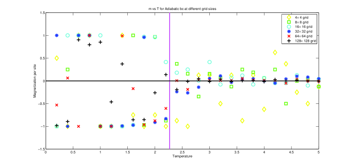
Figure 1: Magnetisation per site vs temperature for the comparison among lattice sizes ($4\times 4$, $8\times 8$, $16\times 16$, $32\times 32$, $64\times 64$ and $128\times 128$) with randomly oriented spin configuration as initial condition and abc. Magenta line represents a parallel line to magnetisation per site at $T=T_{c}$.

We have considered similar simulation procedure to find the optimal $t_{max}$ with lattice size $64\times 64$ for different $t_{max}$ i.e., $2^{13}$, $2^{14}$, $2^{15}$, $2^{16}$, $2^{17}$ and $2^{18}$. One of the simulation result given in figure  2 shows that $t_{max}=2^{17}$ is the best.

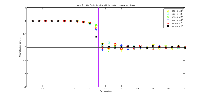
Figure 2: Magnetisation per site vs temperature for the comparison among different $t_{max}$ i.e., $2^{13}$, $2^{14}$, $2^{15}$, $2^{16}$, $2^{17}$ and $2^{18}$ at all down spin initial condition and abc. Magenta line represents a parallel line to magnetisation per site at $T=T_{c}$.

3.2 Phase transition with pbc, abc, rbc, f1bc and f-1bc

In this simulation, we have considered $64\times 64$ lattice size and $t_{max}=2^{17}$ with all bcs and the temperature ranging from $0.1$ to $5.0$ with increment of $0.1$ unit. In figure 3, we have plotted $\bf e$ vs $\bf T$, $\bf m$ vs $\bf T$, $\bf m$ vs $\bf e$, $\bf\chi$ vs $\bf T$, $\bf C_{v}$ vs $\bf T$ and $\bf S$ vs $\bf T$ with initial condition all up with all bcs. Figures 4 and 5 show similar plots with initial condition all down and random spin configuration respectively. We compare, the simulation result of magnetisation with all five bcs with all three initial conditions with the exact solution given by Onsager which are shown in $m$ vs $T$ graphs in figures 3(a), 4(a) and 5(a). Between temperature $T=2$ and $T=2.5$, one finds that the energy gradually increases, magnetisation gradually decreases to zero. The susceptibility and specific heat also change, initially they increase up to $T_{c}$ and then start decreasing as shown in figures 3(d), 4(d), 5(d) and 3(e), 4(e), 5(e) respectively. Entropy gradually increases between temperature $T=2$ and $T=2.5$ and the stays at maximum which are shown in figures 3(f), 4(f) and 5(f). So, a phase transition is clearly visible in between $T=2$ and $T=2.5$ with all three initial conditions with all five bcs. In $m$ vs $e$ graphs shown in figures 3(c), 4(c) and 5(c), the higher density states indicate four states. We find two low temperature ground states around ($M=\pm 1$, $E=-4$) with all three initial conditions and all five bcs. The high temperature phase is centered at ($M=0$, $E=-1$) with all three initial conditions with all five bcs. Then the other state is around ($M=0$, $E=-3.5$), which is a low-temperature metastable states with all five bcs and this happens only in case of random initial condition. With initial condition all up spins and f-1bc, one can find ground state at ($M=-1$, $E=-4$) and for other bcs at ($M=+1$, $E=-4$) and with initial condition all down spins and f1bc, one can find ground state at ($M=+1$, $E=-4$) and for other bcs at ($M=-1$, $E=-4$).

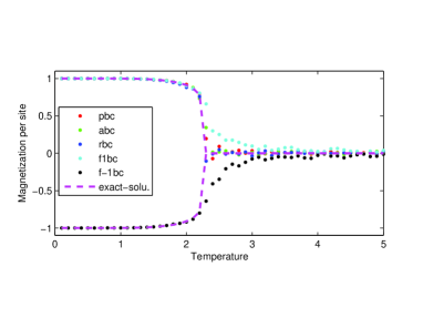
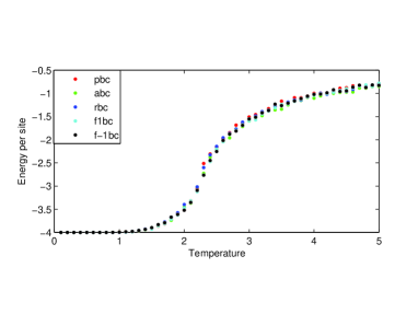
(a)	(b)
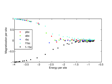
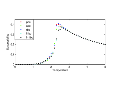
(c)	(d)
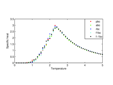
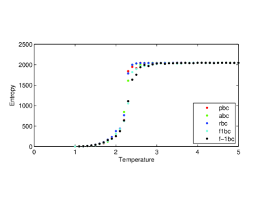
(e)	(f)

Figure 3: (a) $m$ versus $T$ for all bcs, (b) $e$ versus $T$ for all bcs, (c) $m$ versus $e$ for all bcs, (d) $\chi$ versus $T$ for all bcs, (e) $C_{v}$ versus $T$ for all bcs and (f) $S$ versus $T$ for all bcs. Initial condition with all up spin configuration for all five bcs.

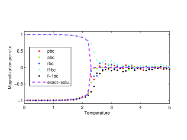
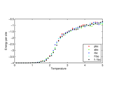
(a)	(b)
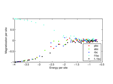
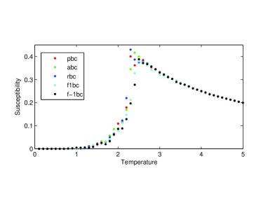
(c)	(d)
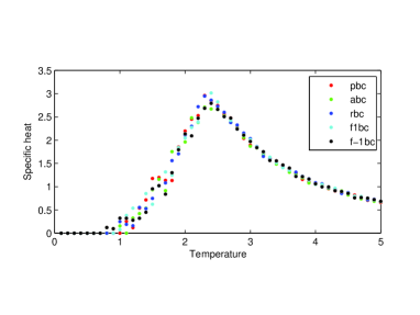
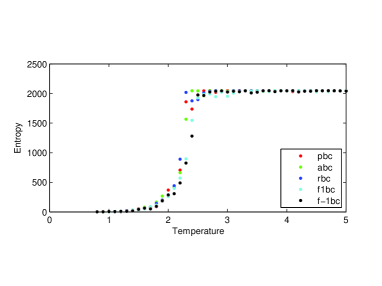
(e)	(f)

Figure 4: (a) $m$ versus $T$ for all bcs, (b) $e$ versus $T$ for all bcs, (c) $m$ versus $e$ for all bcs, (d) $\chi$ versus $T$ for all bcs, (e) $C_{v}$ versus $T$ for all bcs and (f) $S$ versus $T$ for all bcs. Initial condition with all down spin configuration for all five bcs.

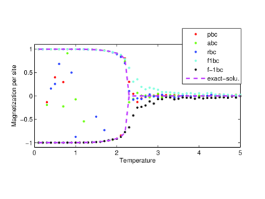
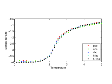
(a)	(b)
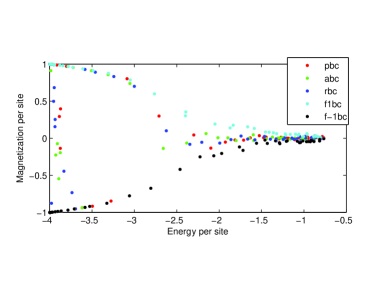
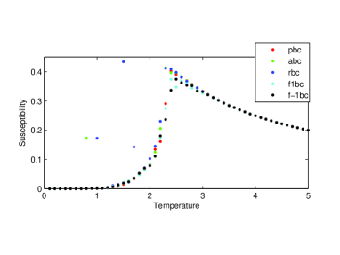
(c)	(d)
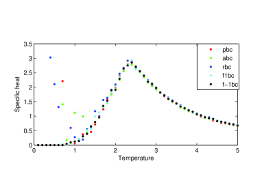
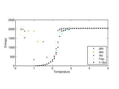
(e)	(f)

Figure 5: (a) $m$ versus $T$ for all bcs, (b) $e$ versus $T$ for all bcs, (c) $m$ versus $e$ for all bcs, (d) $\chi$ versus $T$ for all bcs, (e) $C_{v}$ versus $T$ for all bcs and (f) $S$ versus $T$ for all bcs. Initial condition with random spin configuration for all five bcs.

4 Comparison among Boundary Conditions

Starting with three different initial conditions, from figure 2, one finds that the magnetisation meet the zero line after $T>T_{c}$ differently which is closer to the exact solution in all bcs.

With one simulation for all bcs, it is not possible to predict which bc is closer to $T_{c}$. So, we analyse the points for magnetisation in the range $-0.1\leq m\leq 0.1$ and $-0.2\leq m\leq 0.2$ which are close to the zero line of magnetization (where magnetisation is zero) after $T>T_{c}$. We call such points as converging points.

For the above purpose, we have taken different lattice sizes ranging from $5\times 5$ to $60\times 60$ with increment of $5$; from $60\times 60$ to $100\times 100$ with increment of $10$ and temperature ranging from $0.1$ to $5.0$ with small increment of $0.05$ units. We have considered $t_{max}=2^{15}$ for lattice size $\leq 30\times 30$ and $t_{max}=2^{17}$ for lattice size $>30\times 30$. Figure 6 shows converging points in the above mentioned range of $m$. We have counted the number of converging points as defined above. Their average percentage have calculated by taking average of ten simulations result of each bc with three different initial conditions.

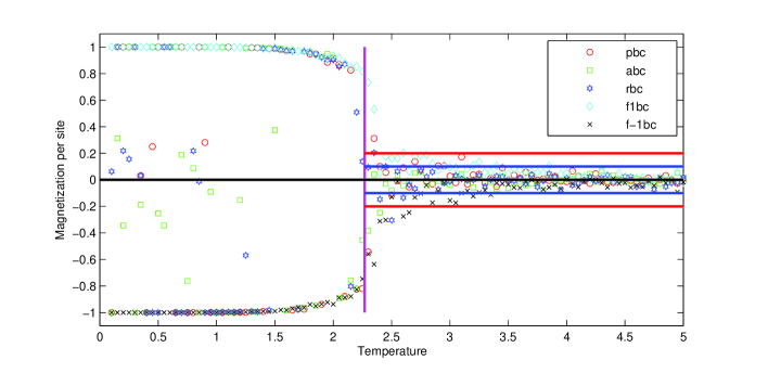
Figure 6: Converging points of bcs for $60\times 60$ lattice size after $T>T_{c}$. Red lines are for magnetisation $m=+0.2$ and $m=-0.2$ and blue lines are for magnetisation $m=+0.1$ and $m=-0.1$ with the initial condition of random spin configuration. Magenta line represents a parallel line to magnetisation per site at $T=T_{c}$.

Lattice $size\leq 30\times 30$ with pbc, abc and rbc, one finds more convergent points in both cases $-0.1\leq m\leq 0.1$ and $-0.2\leq m\leq 0.2$ than f1bc and f-1bc but among the three rbc shows more converging points in all three initial conditions. With lattice size between $30\times 30$ and $70\times 70$ with pbc, abc, rbc, one finds more convergent points in both the cases $-0.1\leq m\leq 0.1$ and $-0.2\leq m\leq 0.2$ in comparison to f1bc and f-1bc with random initial case. For all initial cases with $-0.1\leq m\leq 0.1$, the result is better for pbc, abc and rbc. For $-0.2\leq m\leq 0.2$, the results are better for f1bc with initial condition all down spins and f-1bc with initial condition all up spins. For lattice size greater than $70\times 70$ and less than equal to $100\times 100$ with initial conditions of all up spins and f-1bc and initial condition of all down spins and f1bc, one observe more converging points in both cases $-0.1\leq m\leq 0.1$ and $-0.2\leq m\leq 0.2$. For random initial condition with pbc, rbc and abc, one finds more converging points in both the range of magnetisation per site.

5 Conclusion

We have observed a second order phase transition with respect to all boundary conditions considering all the initial conditions around the critical temperature $T_{c}$. This implies that with the different initial conditions on different lattice sizes $\leq 30\times 30$, one can take care of boundary spins by not only pbc but also by abc and rbc. Further in our analysis, rbc shows more converging points than pbc and rbc for lattice size $\leq 30\times 30$. For lattice size greater than $70\times 70$, f1bc and f-1bc are better suited to use than other bcs in case of initial spin configuration with all up or all down spins. It is also observed that, in case of random initial spin configuration, it is better to use either pbc, abc or rbc when the lattice size is $\leq 100\times 100$. It will be interesting to study the behaviour of all five bcs for lattice $size>100^{2}$ with all initial conditions. Further, also study the phase transition with different values of $t_{max}$ for different lattice sizes. From the simulation point of view, our method takes lesser time than the Metropolis algorithm [5]. This observation is expected to find the approximate values of the critical exponents more accurately. Here, one can reduce the simulation time by generating random numbers using deterministic CA.

Acknowledgement

Work of JM is supported by UGC under the Basic Scientific Research (BSR) scheme. We thank K. Maharana and S. Pattanayak for useful discussions.

References

- [1] L. Onsager, Crystal statistics. I. A two dimensional model with an order-disorder transition,Phys. Rev. 65, 117-149 (1944).
- [2] R. Kotecky and I. Medved, Finite Size Scaling for the 2d Ising model with minus boundary condition, J. Stat. Phys., 104, 905–943 (2001).
- [3] B. M. McCoy and T. T. Wu, The two-dimensional Ising model, Harvard University Press, Cambridge, Massachusetts, (1973).
- [4] N. H. Packard and S. Wolfram, Two-Dimensional Cellular Automata, J. Stat. Phys., 38, 5/6 (1985).
- [5] N. Metropolis, A. W. Rosenbluth, M. N. Rosenbluth, A. H. Teller and E. Teller, Equation of state calculations by fast computing machines, The Journal of Chemical Physics, 21(6), 1087–1092 (1953).
- [6] W. Ulli, Collective Monte Carlo Updating for Spin Systems, Phys. Rev. Lett., 62(4), 361 (1989).
- [7] B. Zheng, Monte Carlo simulations of short-time critical dynamics, Int. J. Mod. Phys., B12, 1419-1484 (1998).
- [8] E. Domany and W. Kinzel, Equivalence of Cellular Automata to Ising Models and Directed Percolation, Phys. Rev. Lett., 53, 4 (1984).
- [9] G. Y. Vichniac, Simulating physics with cellular automata, Physica D., 10, 96-116 (1984).
- [10] J. G. Zabolitzky and H. J. Herrmann, Multitasking case study on the Cray-2: The Q2R cellular automaton, J. Comp. Phys., 76, 426-447 (1988).
- [11] D. Stauffer, Critical 2D and 3D Dynamics of Q2R Cellular Automata, Comp. Phys. Comm., 127, 113-119 (2000).
- [12] S. Kremer and D. E. Wolf, Numerical method for analyzing surface fluctuations, Physica A, 182, 542-556 (1992).
- [13] C. Moukarzel and N. Parga, On the evaluation of magnetisation fluctuations with Q2R cellular automata, J. Phys. A, 22, 943 (1989).
- [14] M. Creutz, Deterministic ising dynamics, Ann. Phys., 167(1), 62-72 (1986).
- [15] N. Aktekin, Simulation of the three-dimensional Ising model on the Creutz cellular automaton, Physica A, 219, 3-4, 436-446 (1995).
- [16] N. Aktekin, Simulation of the four-dimensional Ising model on the Creutz cellular automaton, Physica A, 232, 1-2, 397-407 (1996).
- [17] N. Aktekin, Simulation of the Eight-Dimensional Ising Model on the Creutz Cellular Automaton, Int. J. Mod. Phys. C, 8(2), 287-292 (1997).
- [18] Y. Asgari and M. Ghaemi, Obtaining critical point and shift exponent for the anisotropic two-layer Ising and Potts models: Cellular automata approach, Physica A, 387, 8-9, 1937-1946 (2008).