Transverse exponential stability and applications

Abstract

We investigate how the following properties are related to each other: i) - A manifold is “transversally” exponentially stable; ii) - The “transverse” linearization along any solution in the manifold is exponentially stable; iii) - There exists a field of positive definite quadratic forms whose restrictions to the directions transversal to the manifold are decreasing along the flow. We illustrate their relevance with the study of exponential incremental stability. Finally, we apply these results to two control design problems, nonlinear observer design and synchronization. In particular, we provide necessary and sufficient conditions for the design of nonlinear observer and of nonlinear synchronizer with exponential convergence property.

1 Introduction

The property of attractiveness of a (non-trivial) invariant manifold is often sought in many control design problems. In the classical internal model based output regulation [16], it is known that the closed-loop system must have an attractive invariant manifold, on which, the tracking error is equal to zero. In the Immersion & Invariance [6], in the sliding-mode control approaches, or observer designs [3], obtaining an attractive manifold is an integral part of the design procedure. Many multi-agent system problems, such as, formation control, consensus and synchronization problems, are also closely related to the analysis and design of an attractive invariant manifold, see, for example, [8, 29, 34].

The study of stability and/or attractiveness of invariant manifolds and more generally of sets has a long history. See for instance [35, §16] and the references therein. In this paper, we focus on the exponential convergence property by studying the system linearized transversally to the manifold. We show that this attractiveness property is equivalent to the existence of positive definite quadratic forms which are decreasing along the flow of the transversally linear system. For constant quadratic forms and when the system has some specific structure, the latter becomes the Demidovich criterion which is a sufficient, but not yet necessary, condition for convergent systems [22, 23, 25]. On the other hand, if we consider the standard output regulation theory as pursued in [16], the attractiveness of the invariant manifold is established using the center manifold theorem which corresponds to the stability property of the linearized system at an equilibrium point. Due to the lack of characterization of an attractive invariant manifold, most of the literature on constructive design for nonlinear output regulator is based on various different sufficient conditions that can be very conservative. In these regards, our main results can potentially provide a new framework for control designs aiming at making an invariant manifold attractive.

The paper is divided into two parts. In Subsection 2.1, we study a dynamical system that admits a transverse exponentially stable invariant manifold. In particular, we establish equivalent relations between:

• the transverse exponential stability of an invariant manifold;

• the exponential stability of the transverse linearized system;

• the existence of field of positive definite quadratic forms the restrictions to the transverse direction to the manifold of which are decreasing along the flow.

We illustrate these results by considering a particular case of exponential incremental stable systems in Subsection 2.2. Here, incremental stability refers to the property where the distance between any two trajectories converges to zero (see, for example, [4, 12, 5]). For such systems, the property (i) $\Leftrightarrow$ (iii) is used to prove that the exponential incremental stability property is equivalent to the existence of a Riemannian distance which is contracted by the flow.

In the second part of the paper, we apply the equivalence results to two different control problems: nonlinear observer design and synchronization of nonlinear multi-agent systems. In both problems, a necessary condition is obtained. Based on this necessary condition, we propose a novel design for an observer, in Subsection 3.1, and for a synchronizer, in Subsection 3.2.

In Subsection 3.1, we reinterpret the three properties (i), (ii) and (iii) in the context of observer design. This allows us to revisit some of the results obtained recently in [27] and [1] and, more importantly, to show that the sufficient condition given in [27] is actually also a necessary condition to design an exponential (local) full-order observer.

Finally, in Subsection 3.2, we solve a nonlinear synchronization problem. In particular, we give some necessary and sufficient conditions to achieve (local) exponential synchronization of nonlinear multi-agent systems involving more than two agents. This result generalizes our preliminary work in [2]. Moreover, under an extra assumption, we show how to obtain a global synchronization for the two agents case.

It is worth noting that our main results are applicable to other control problems beyond the two control problems mentioned before. In a recent paper by Wang, Ortega & Su [33], our results have been applied to solve an adaptive control problem via the Immersion & Invariance principle.

2 Main result

2.1 Transversally exponentially stable manifold

Throughout this section, we consider a system in the form

$$\dot{e}=F(e,x)\ ,\quad\dot{x}=G(e,x)$$ (1)

where $e$ is in ${\mathbb{R}}^{n_{e}}$, $x$ is in ${\mathbb{R}}^{n_{x}}$ and the functions $F:{\mathbb{R}}^{n_{e}}\times{\mathbb{R}}^{n_{x}}\rightarrow{\mathbb{R}}^{n_{e}}$ and $G:{\mathbb{R}}^{n_{e}}\times{\mathbb{R}}^{n_{x}}\rightarrow{\mathbb{R}}^{n_{x}}$ are $C^{2}$. We denote by $(E(e_{0},x_{0},t),X(e_{0},x_{0},t))$ the (unique) solution which goes through $(e_{0},x_{0})$ in ${\mathbb{R}}^{n_{e}}\times{\mathbb{R}}^{n_{x}}$ at time $t=0$. We assume it is defined for all positive times, i.e. the system is forward complete.

The system (1) above can be used, for example, to study the behavior of two distinct solutions $X(x_{1},t)$ and $X(x_{2},t)$ of the system defined on ${\mathbb{R}}^{n}$ by

$$\dot{x}=f(x)$$ (2)

Indeed, we obtain an $(e,x)$-system of the type (1) with

$$F(e,x)=f(x+e)-f(x)\ ,\quad G(e,x)=f(x)\ .$$ (3)

This is the context of incremental stability that we will use throughout this section to illustrate our main results.

In the following, to simplify our notations, we denote by $B_{e}(a)$ the open ball of radius $a$ centered at the origin in ${\mathbb{R}}^{n_{e}}$.

We study the links between the following three notions.

• (Transversal uniform local exponential stability)
  The system (1) is forward complete and there exist strictly positive real numbers $r$, $k$ and $\lambda$ such that we have, for all $(e_{0},x_{0},t)$ in $B_{e}(r)\times{\mathbb{R}}^{n_{x}}\times{\mathbb{R}}_{\geq 0}$,

  $$|E(e_{0},x_{0},t)|\leq k|e_{0}|\exp(-\lambda t)\ .$$ (4)

• (Uniform exponential stability for the transversally linear system)
  The system

  $$\dot{{\widetilde{x}}}={\widetilde{G}}({\widetilde{x}}):=G(0,{\widetilde{x}})$$ (5)

  is forward complete and there exist strictly positive real numbers ${\widetilde{k}}$ and $\tilde{\lambda}$ such that any solution $({\widetilde{E}}({\widetilde{e}}_{0},{\widetilde{x}}_{0},t),{\widetilde{X}}({\widetilde{x}}_{0},t))$ of the transversally linear system

  $$\dot{\widetilde{e}}=\frac{\partial F}{\partial e}(0,{\widetilde{x}}){\widetilde{e}}\ ,\quad\dot{\widetilde{x}}={\widetilde{G}}({\widetilde{x}})$$ (6)

  satisfies, for all $({\widetilde{e}}_{0},{\widetilde{x}}_{0},t)$ in ${\mathbb{R}}^{n_{e}}\times{\mathbb{R}}^{n_{x}}\times{\mathbb{R}}_{\geq 0}$,

  $$|{\widetilde{E}}({\widetilde{e}}_{0},{\widetilde{x}},t)|\leq{\widetilde{k}}\exp(-\tilde{\lambda}t)|{\widetilde{e}}_{0}|\ .$$ (7)

• (Uniform Lyapunov matrix transversal equation)
  For all positive definite matrix $Q$, there exists a continuous function ${P}:{\mathbb{R}}^{n_{x}}\rightarrow{\mathbb{R}}^{n_{e}\times n_{e}}$ and strictly positive real numbers $\underline{p}$ and $\overline{p}$ such that ${P}$ has a derivative ${\mathfrak{d}}_{{\widetilde{G}}}{P}$ along ${\widetilde{G}}$ in the following sense

  $${\mathfrak{d}}_{{\widetilde{G}}}{P}({\widetilde{x}})\;:=\;\lim_{h\to 0}\frac{{P}({\widetilde{X}}({\widetilde{x}},h))-{P}({\widetilde{x}})}{h}$$ (8)

  and we have, for all ${\widetilde{x}}$ in ${\mathbb{R}}^{n_{x}}$,

  $$\displaystyle\hskip-30.00005pt{\mathfrak{d}}_{{\widetilde{G}}}{P}({\widetilde{x}})+{P}({\widetilde{x}})\frac{\partial F}{\partial e}(0,{\widetilde{x}})+\frac{\partial F}{\partial e}(0,{\widetilde{x}})^{\prime}{P}({\widetilde{x}})\leq-Q$$ (9)

  $$\displaystyle\underline{p}\,I\leq{P}({\widetilde{x}})\leq\overline{p}\,I\ .$$ (10)

In other words, the system (1) is said to be TULES-NL if the manifold $\mathcal{E}:=\{(e,x):\,e=0\}$ is exponentially stable for the system (1), locally in $e$ and uniformly in $x$; and it is said to be UES-TL if the manifold $\tilde{\mathcal{E}}:=\{({\widetilde{x}},{\widetilde{e}}):\,{\widetilde{e}}=0\}$ of the linearized system transversal to $\mathcal{E}$ in (6) is exponentially stable uniformly in ${\widetilde{x}}$.

Concerning the ULMTE property, condition (9) is related to the notion of horizontal contraction introduced in [11, Section VII]). However a key difference is that we do not require the monotonicity condition (9) to hold in the whole manifold ${\mathbb{R}}^{n_{e}}\times{\mathbb{R}}^{n_{x}}$ but only along the invariant submanifold $\mathcal{E}$. In this case the corresponding horizontal Finsler-Lyapunov function $V:\left({\mathbb{R}}^{n_{x}}\times{\mathbb{R}}^{n_{e}}\right)\times\left({\mathbb{R}}^{n_{x}}\times{\mathbb{R}}^{n_{e}}\right)$ that we get takes the form $V((x,e),(\delta_{x},\delta_{e}))=\delta_{e}^{\prime}P(x)\delta_{e}$.

In the case where the manifold is reduced to a single point, i.e. when the system (1) is simply $\dot{e}=F(e)$ with an equilibrium point at the origin (i.e. $F(0)=0$) then

• the TULES-NL property can be understood as the local exponential stability of the origin;

• the UES-TL notion translates to the exponential stability of the linear system $\dot{\widetilde{e}}=\frac{\partial F}{\partial e}(0){\widetilde{e}}$; and

• the ULMTE concept is about the existence of a positive definite matrix $P$ solution to the Lyapunov equation $P\frac{\partial F}{\partial e}(0)+\frac{\partial F}{\partial e}(0)^{\top}P=-Q$ where $Q$ is an arbitrary positive definite matrix.

In this particular case it is well known that these three properties are equivalent.

For the example of incremental stability, as mentioned before, the three properties of TULES-NL, UES-TL and ULMTE can be understood globally as follows :

• System (2) is globally exponentially incrementally stable. Namely there exist two strictly positive real numbers $k$ and $\lambda$ such that for all $(x_{1},x_{2})$ in ${\mathbb{R}}^{n}\times{\mathbb{R}}^{n}$ we have, for all $t$ in ${\mathbb{R}}_{\geq 0}$,

  $$|X(x_{1},t)-X(x_{2},t)|\leq k|x_{1}-x_{2}|\exp(-\lambda t).$$ (11)

• The manifold $\mathcal{E}=\{(x,e),e=0\}$ is globally exponentially stable for the system

  $$\dot{e}=\frac{\partial f}{\partial x}(x)e\ ,\quad\dot{x}=f(x)$$ (12)

  Namely there exist two strictly positive real numbers $k_{e}$ and $\lambda_{e}$ such that for all $(e,x)$ in ${\mathbb{R}}^{n}\times{\mathbb{R}}^{n}$, the corresponding solution of (12) satisfies

  $$|E(e,x,t)|\leq k_{e}|e|\exp(-\lambda_{e}t)\ ,\ \forall t\in{\mathbb{R}}_{\geq 0}\ .$$

• There exists a positive definite matrix $Q$ in ${\mathbb{R}}^{n\times n}$, a $C^{2}$ function $P:{\mathbb{R}}^{n}\rightarrow{\mathbb{R}}^{n\times n}$ and strictly positive real numbers $\underline{p}$ and $\overline{p}$ such that $P$ has a derivative ${\mathfrak{d}}_{f}P$ along $f$ in the sense of (22) ,and satisfies (21) and(19).

In this context it is known that P3 $\Rightarrow$ P1. Actually asymptotic incremental stability for which Property P1 is a particular case is known to be equivalent to the existence of an appropriate Lyapunov function. This has been established in [36, 32, 4] or [25] for instance. In our context, this Lyapunov function is given as a Riemannian distance. We shall show below that, as for the case of an equilibrium point, we have also P1 $\Rightarrow$ P2 $\Rightarrow$ P3, (see Proposition 4), namely incremental exponential stability implies the existence of a Riemannian distance for which the flow is contracting.

In studying the equivalence relation between TULES-NL,UES-TL and ULMTE, we are not interested in the possibility of a solution near the invariant manifold to inherit some properties of solutions in this manifold, such as, the asymptotic phase, the shadowing property, the reduction principle, etc., nor in the existence of some special coordinates allowing us to exhibit some invariant splitting in the dynamics (exponential dichotomy). This is the reason that, besides forward completeness, we assume nothing for the in-manifold dynamics given by :

$$\dot{\tilde{x}}={\widetilde{G}}(\tilde{x})=G(0,\tilde{x})\ .$$

So, for not misleading our reader, we prefer to use the word “transversal” instead of “normal” as seen for instance in the various definitions of normally hyperbolic submanifolds given in [14, §1].

In order to simplify the exposition of our results and to concentrate our attention on the main ideas, we assume everything is global and/or uniform, including restrictive bounds. Most of this can be relaxed with working on open or compact sets, but then with restricting the results to time intervals where a solution remains in such a particular set.

2.1.1 TULES-NL “$\Rightarrow$” UES-TL

In the spirit of Lyapunov first method, we have the following result.

Proposition 1.

If Property TULES-NL holds and there exist positive real numbers $\rho$, $\mu$ and $c$ such that, for all $x$ in ${\mathbb{R}}^{n_{x}}$,

$$\left|\frac{\partial F}{\partial e}(0,x)\right|\leq\mu\ ,\quad\left|\frac{\partial G}{\partial x}(0,x)\right|\leq\rho$$ (13)

and, for all $(e,x)$ in $B_{e}(kr)\times{\mathbb{R}}^{n_{x}}$,

$$\left|\frac{\partial^{2}F}{\partial e\partial e}(e,x)\right|\leq c\ ,\ \left|\frac{\partial^{2}F}{\partial x\partial e}(e,x)\right|\leq c\ ,\ \left|\frac{\partial G}{\partial e}(e,x)\right|\leq c\;,$$ (14)

then Property UES-TL holds.

The proof of this proposition is given in Appendix .1. Roughly speaking, it is based on the comparison between a given $e$-component of a solution ${\widetilde{E}}({\widetilde{e}}_{0},{\widetilde{x}}_{0},t)$ of (6) with pieces of $e$-component of solutions $E({\widetilde{e}}_{i},{\widetilde{x}}_{i},t-t_{i})$ of solutions of (1) where ${\widetilde{e}}_{i},{\widetilde{x}}_{i}$ are sequences of points defined on ${\widetilde{E}}({\widetilde{e}}_{0},{\widetilde{x}}_{0},t)$. Thanks to the bounds (13) and (14), it is possible to show that ${\widetilde{E}}$ and $E$ remain sufficiently closed so that ${\widetilde{E}}$ inherit the convergence property of the solution $E$. As a consequence, in the particular case in which $F$ does not depend on $x$, the two functions $E$ and ${\widetilde{E}}$ do not depend on $x$ either and the bounds on the derivatives of the $G$ function are useless.

2.1.2 UES-TL “$\Rightarrow$” ULMTE

Analogous to the property of existence of a solution to the Lyapunov matrix equation, we have the following proposition on the link between UES-TL and ULMTE notions.

Proposition 2.

If Property UES-TL holds and there exists a positive real number $\mu$ such that

$$\left|\frac{\partial F}{\partial e}(0,x)\right|\leq\mu\qquad\forall x\in{\mathbb{R}}^{n_{x}}\ ,$$ (15)

then Property ULMTE holds.

The proof of this proposition is given in Appendix .2. The idea is to show that, for every symmetric positive definite matrix $Q$, the function ${P}:{\mathbb{R}}^{n_{x}}\rightarrow{\mathbb{R}}^{n_{e}\times n_{e}}$ given by

$${P}({\widetilde{x}})=\lim_{T\to+\infty}\int_{0}^{T}\left(\frac{\partial{\widetilde{E}}}{\partial{\widetilde{e}}}(0,{\widetilde{x}},s)\right)^{\prime}Q\frac{\partial{\widetilde{E}}}{\partial{\widetilde{e}}}(0,{\widetilde{x}},s)ds$$ (16)

is well defined, continuous and satisfies all the requirements of the property ULMTE. The assumption (15) is used to show that $P$ satisfies the left inequality in (10). Nevertheless this inequality holds without (15) provided the function $s\mapsto\left|\frac{\partial{\widetilde{E}}}{\partial{\widetilde{e}}}(0,{\widetilde{x}},s)\right|$ does not go too fast to zero.

2.1.3 ULMTE “$\Rightarrow$” TULES-NL

Proposition 3.

If Property ULMTE holds and there exist positive real numbers $\eta$ and $c$ such that, for all $(e,x)$ in $B_{e}(\eta)\times{\mathbb{R}}^{n_{x}}$,

$$\displaystyle\left|\frac{\partial P}{\partial x}(x)\right|\leq c\;,$$ (17)

$$\hskip-16.00008pt\displaystyle\left|\frac{\partial^{2}F}{\partial e\partial e}(e,x)\right|\leq c\;,\ \left|\frac{\partial^{2}F}{\partial x\partial e}(e,x)\right|\leq c\;,\ \left|\frac{\partial G}{\partial e}(e,x)\right|\leq c\,,\hbox{}$$ (18)

then Property TULES-NL holds.

The proof of this proposition can be found in Appendix .3. This is a direct consequence of the use of $V(e,x)=e^{\prime}P(x)e$ as a Lyapunov function. The bounds (17) and (18) are used to show that, with equation (9), the time derivative of this Lyapunov function is negative in a (uniform) tubular neighborhood of the manifold $\{(e,x),e=0\}$.

2.2 Revisiting the exponential incremental stable systems

Incremental stability of an autonomous system (2) is the property that a distance between any two solutions of (2) converges asymptotically to zero. The characterization of it has been studied thoroughly, for example, in [4, 12, 5]. In [4, 5], a Lyapunov characterization of incremental stability ($\delta$-GAS for autonomous systems and $\delta$-ISS for non-autonomous ones) is given based on the Euclidean distance between two states that evolve in an identical system. A variant of this notion is that of convergent systems discussed in [22, 25]. All these studies are based on the notion of contracting flows which has been widely studied in the literature and for a long time, see, for example, [18, 19, 13, 9, 21, 20, 11]. These flows generate trajectories between which an appropriately defined distance is monotonically decreasing with increasing time. See [17] for a historical discussion on the contraction analysis and [30] for a partial survey.

The big issue in this view points is to find the appropriate distance which may be a difficult task. The results in Section 2 may help in this regard with providing an explicit construction of a Riemannian distance.

Precisely, let $P$ be a $C^{2}$ function defined on ${\mathbb{R}}^{n}$ the values of which are symmetric matrices satisfying

$$\underline{p}\,I\leq P(x)\leq\overline{p}\,I\qquad\forall x\in{\mathbb{R}}^{n}$$ (19)

The length of any piece-wise $C^{1}$ path $\gamma:[s_{1},s_{2}]\to{\mathbb{R}}^{n}$ between two arbitrary points $x_{1}=\gamma(s_{1})$ and $x_{2}=\gamma(s_{2})$ in ${\mathbb{R}}^{n}$ is defined as :

$$\left.L(\gamma)\vrule height=5.09995pt,depth=5.09995pt,width=0.0pt\right|_{s_{1}}^{s_{2}}=\int_{s_{1}}^{s_{2}}\sqrt{\frac{d\gamma}{ds}(\sigma)^{\prime}P(\gamma(\sigma))\frac{d\gamma}{ds}(\sigma)}\>d\sigma$$ (20)

By minimizing along all such path we get the distance $d(x_{1},x_{2})$.

Then, thanks to the well established relation between (geodesically) monotone vector field (semi-group generator) (operator) and contracting (non-expansive) flow (semi-group) (see [18, 13, 7, 15] and many others), we know that this distance between any two solutions of (2) is exponentially decreasing to $0$ as time goes on forward if we have

$${\mathfrak{d}}_{f}P(x)+P(x)\frac{\partial f}{\partial x}(x)+\frac{\partial f}{\partial x}(x)^{\prime}P(x)\leq-Q\qquad\forall x\in{\mathbb{R}}^{n}\ ,$$ (21)

where $Q$ is a positive definite symmetric matrix and

$${\mathfrak{d}}_{f}P(x)\;=\;\lim_{h\to 0}\frac{P(X(x,h))-P(x)}{h}\ .$$ (22)

For a proof, see for example [18, Theorem 1] or [15, Theorems 5.7 and 5.33] or [24, Lemma 3.3] (replacing $f(x)$ by $x+hf(x)$).

In this context, using the main results of our previous section, we can show that, if we have exponential incremental stability, then there exists a function $P$ meeting the above requirements. Specifically, we have the following proposition.

Proposition 4 (Incremental stability).

Assume the system (2) is forward complete with a function $f$ which is $C^{3}$ with bounded first, second and third derivatives. Let $X(x,t)$ denotes its solutions. Then we have P1 $\Rightarrow$ P2 $\Rightarrow$ P3 (and therefore P1 $\Leftrightarrow$ P2 $\Leftrightarrow$ P3).

In other words, exponential incremental stability property is equivalent to the existence of a Riemannian distance which is contracted by the flow and can be used as a $\delta$-GAS Lyapunov function. Note also that, despite the fact that the main results in Section 2 are local, when we restrict ourselves to the incremental stability problem, we can obtain a global result.

Proof : P1 $\Rightarrow$ P2 $\Rightarrow$ P3: Consider the system (3) and let $n_{x}=n_{e}=n$. The boundedness of the first derivative of $f$ implies the forward completeness of the corresponding systems (1) and (5). Moreover the inequalities (13), (14) and (15) with $r=+\infty$ follow from the assumption of boundedness of the derivatives of $f$.

As a consequence P1$\Rightarrow$ P2 follows from Proposition 1 and P2$\Rightarrow$ P3 from Proposition 2. Note however that it remains to show that $P$ defined in (16) is $C^{2}$. This is obtained employing the boundedness of the first, second and third derivatives of $f$. Indeed, note that we have for all $(t,x)$ $\frac{\partial{\widetilde{E}}}{\partial e}(0,x,t)=\frac{\partial X}{\partial x}(x,t)$. So to show that $P$ is $C^{1}$ it suffices to show that the mapping $t\mapsto\frac{\partial^{2}X}{\partial x_{i}\partial x}(x,t)$ goes exponentially to zero as time goes to infinity. Note that this is indeed the case since given a vector $v$ in ${\mathbb{R}}^{n}$ and $i$ in $\{1,\dots,n\}$ the mapping $\nu(t)=\frac{\partial^{2}X}{\partial x_{i}\partial x}(x,t)v$ is solution to

$$\dot{\nu}=\frac{\partial f}{\partial x}(X(x,t))\nu+\\ \sum_{j=1}^{n}\frac{\partial^{2}f}{\partial x_{j}\partial x}(X(x,t))\frac{\partial X_{j}}{\partial x_{i}}(x,t)\frac{\partial X}{\partial x}(x,t)v$$

Hence, from (21), (19) and the fact that $f$ has bounded second derivatives, it yields the existence of a positive real number $\tilde{c}$ such that

$$\dot{\mathop{\vbox{\halign{#\cr\crcr\kern 1.72218pt\cr$\braceld\leaders\vrule\hfill\bracerd$\crcr\kern 1.72218pt\nointerlineskip\cr$\hfil\displaystyle{\nu^{\prime}P(X(x,t))\nu}\hfil$\crcr}}}\limits}\leq-\nu^{\prime}Q\nu+\tilde{c}|\nu|\left|\frac{\partial X}{\partial x}(x,t)\right|^{2}\ .$$

Since $t\mapsto\frac{\partial X}{\partial x}(x,t)$ exponentially goes to zero as time goes to infinity, it implies that $\nu$ exponentially goes to zero. Hence, $P$ is $C^{1}$. Employing the bound on the third derivative and following the same route, it follows that $P$ is $C^{2}$. $\Box$

3 Applications

In this section, we apply Propositions 1, 2 and 3 in two different contexts: full order observer and synchronization.

3.1 Nonlinear observer design

Consider a system

$$\dot{x}=f(x)\ ,\quad y=h(x)\ .$$ (23)

with state $x$ in ${\mathbb{R}}^{n}$ and output $y$ in ${\mathbb{R}}^{p}$ augmented with a state observer of the particular form

$$\dot{\hat{x}}=f(\hat{x})+K(y,\hat{x})$$ (24)

with state $\hat{x}$ in ${\mathbb{R}}^{n}$ and where

$$K(h(x),x)\;=\;0\qquad\forall x\ .$$ (25)

Assuming the functions $f$, $h$ and $K$ are $C^{2}$, we are interested in having the manifold $\{(x,\hat{x}):\,x=\hat{x}\}$ exponentially stable for the overall system

$$\dot{x}=f(x)\ ,\quad\dot{\hat{x}}=f(\hat{x})+K(y,\hat{x})\ .$$ (26)

When specified to this context, the properties TULES-NL, UES-TL and ULMTE are

• The system (26) is forward complete and there exist strictly positive real numbers $r$, $k$ and $\lambda$ such that we have, for all $(x,\hat{x},t)$ in ${\mathbb{R}}^{n}\times{\mathbb{R}}^{n_{x}}\times{\mathbb{R}}_{\geq 0}$ satisfying $|x_{0}-\hat{x}_{0}|\leq r$, we have

  $$|X(x_{0},t)-\hat{X}(x_{0},\hat{x}_{0},t)|\leq k|x_{0}-\hat{x}_{0}|\exp(-\lambda t)\ .$$ (27)

• The system

  $$\dot{x}=f(x)$$

  is forward complete and there exist strictly positive real numbers ${\widetilde{k}}$ and $\tilde{\lambda}$ such that any solution $({\widetilde{E}}({\widetilde{e}}_{0},x_{0},t),X(x_{0},t))$ of the transversally linear system

  $$\dot{\widetilde{e}}=\left[\frac{\partial f}{\partial x}(x)+\frac{\partial K}{\partial y}(h(x),x)\frac{\partial h}{\partial x}(x)\right]{\widetilde{e}}\ ,\quad\dot{x}=f(x)$$ (28)

  satisfies, for all $({\widetilde{e}}_{0},x_{0},t)$ in ${\mathbb{R}}^{n}\times{\mathbb{R}}^{n}\times{\mathbb{R}}_{\geq 0}$,

  $$|{\widetilde{E}}({\widetilde{e}}_{0},x_{0},t)|\leq{\widetilde{k}}\exp(-\tilde{\lambda}t)|{\widetilde{e}}_{0}|\ .$$ (29)

• : For all positive definite matrix $Q$, there exists a continuous function ${P}:{\mathbb{R}}^{n}\rightarrow{\mathbb{R}}^{n\times n}$ and strictly positive real numbers $\underline{p}$ and $\overline{p}$ such that we have, for all $x$ in ${\mathbb{R}}^{n}$,

  $$\underline{p}\,I\leq{P}(x)\leq\overline{p}\,I\ ,$$

  $\displaystyle{\mathfrak{d}}_{f}{P}(x)$
  $\displaystyle+\;2\texttt{Sym}\left(\!{P}(x)\!\left[\frac{\partial f}{\partial x}(x)+\frac{\partial K}{\partial y}(h(x),x)\frac{\partial h}{\partial x}(x)\right]\!\right)$ $(30)$
  $\displaystyle\leq-Q\ .\quad$

  
  

  where $\texttt{Sym}(A)=A+A^{\prime}$.

Propositions 1, 2 and 3 give conditions under which these properties are equivalent. But these properties assume the data of the correction term $K$. Hence, by rewriting UES-TEL and TULES-NL in a way in which the design parameter $K$ disappears, these propositions give necessary conditions for the existence of an exponentially convergent observer.

Property UES-TL involves the existence of an observer with correction term depending on $x$ for the time-varying linear system resulting from the linearization along a solution to the system (23), i.e.

$$\dot{\widetilde{e}}=\frac{\partial f}{\partial x}(x){\widetilde{e}}\ ,\quad\tilde{y}=\frac{\partial h}{\partial x}(x){\widetilde{e}}$$ (31)

seeing $\tilde{y}$ as output. As a consequence of Proposition 1, a necessary condition for Property UES-TL to hold and further, when some derivatives are bounded, for the existence of an exponentially convergent observer is that the system (23) be infinitesimally detectable in the following sense

• We say that the system (23) is infinitesimally detectable if every solution of

  $$\dot{x}=f(x)\ ,\quad\dot{\widetilde{e}}=\frac{\partial f}{\partial x}(x){\widetilde{e}}\ ,\ \frac{\partial h}{\partial x}(x){\widetilde{e}}=0$$

  defined on $[0,+\infty)$ satisfies $\lim_{t\rightarrow+\infty}|{\widetilde{E}}(e,x,t)|=0$.

A similar necessary condition has been established in [1] for a larger class of observers but under an extra assumption (the existence of a locally quadratic Lyapunov function).

Example 1: Consider the planar system

$$\dot{x}_{1}\;=\;x_{2}^{3}\ ,\quad\dot{x}_{2}\;=\;-x_{1}\ ,\quad y\;=\;x_{1}\ .$$ (32)

We wish to know whether or not it is possible to design an exponentially convergent observer for this nonlinear oscillator in the form of (24). The linearized system is

$$\dot{\widetilde{e}}_{1}\;=\;3x_{2}^{2}\,{\widetilde{e}}_{2}\ ,\quad\dot{\widetilde{e}}_{2}\;=\;-{\widetilde{e}}_{1}\ ,\quad\tilde{y}\;=\;{\widetilde{e}}_{1}$$ (33)

This system is not detectable when the solution, along which we linearize, is the origin which is an equilibrium of (32). Consequently the system (32) is not infinitesimally detectable on ${\mathbb{R}}^{2}$ and so there is no exponentially convergent observer on ${\mathbb{R}}^{2}$. Fortunately the subset $\{x\in{\mathbb{R}}^{2}:\,\frac{x_{1}^{2}}{2}+\frac{x_{2}^{4}}{4}\geq\epsilon\}$, with $\epsilon>0$, is invariant and (32) is infinitesimally detectable in it.

To design a correction term $K$ for an exponentially convergent observer, we use the property that

$$L(y,x)\;=\;\frac{\partial K}{\partial y}(y,x)$$

should be an observer gain for the linear system (33). So we start our design by selecting $L$. We pick

$$L(y,x)=\begin{bmatrix}-3x_{2}^{2}\\ -3x_{2}^{2}+1\end{bmatrix}$$

This gives (see (28))

$$A(x)\;=\;\frac{\partial f}{\partial x}(x)+\frac{\partial K}{\partial y}(h(x),x)\frac{\partial h}{\partial x}(x)\;=\;3x_{2}\begin{bmatrix}-1&1\\ 0&-1\end{bmatrix}$$

The transition matrix generated by $A(X(x,t))$ when $X(x,t)$ is a solution of (32) is

$$\Phi(t,0)\;=\;\exp\left(-I(t)\right)\begin{bmatrix}1&I(t)\\ 0&1\end{bmatrix}$$

where

$$I(t)\;=\;3\,\int_{0}^{t}X_{2}(x,s)^{2}ds\ .$$

Since $X_{2}(x,t)$ is periodic, (29) holds when the initial condition $x$ is in the compact invariant subset

$$\mathcal{C}\;=\;\{x\in{\mathbb{R}}^{2}:\,\frac{1}{\varepsilon}\geq\frac{x_{1}^{2}}{2}+\frac{x_{2}^{4}}{4}\geq\epsilon\}\ .$$ (34)

Then, according to Propositions 2 and 3, and in view of (25), we obtain an exponentially convergent observer by choosing $K$ as

$$K(y,x)\;=\;\int_{x_{1}}^{y}L(s,x)ds\;=\;\begin{bmatrix}-3x_{2}^{2}\\ -3x_{2}^{2}+1\end{bmatrix}(y-x_{1})\ .$$

Similarly, Property ULMTE involves the existence of $P$ and $K$ such that (ULMTE FOR OBSERVER) holds. By restricting this inequality on quadratic forms to vectors which are in the kernel of $\frac{\partial h}{\partial x}$, we obtain as a consequence of Propositions 1 and 2 that a necessary condition for Property ULMTE to hold and further, when some derivatives are bounded, for the existence of an exponentially convergent observer is that the system (23) be R-detectable (R for Riemann) in the following sense.

• We say that the system (23) is R-detectable if there exist a continuous function ${P}:{\mathbb{R}}^{n}\rightarrow{\mathbb{R}}^{n\times n}$ and positive real numbers $0<\underline{p}\leq\overline{p}$ and $0<\underline{q}$ such that $P$ has a derivative ${\mathfrak{d}}_{f}P$ along $f$ in the sense of (22) and we have

  $$\underline{p}\,I\leq P(x)\leq\overline{p}\,I\qquad\forall x\in{\mathbb{R}}^{n}$$ (35)

  and

  $$v^{\prime}{\mathfrak{d}}_{f}{P}({\widetilde{x}})v+2v^{\prime}{P}({\widetilde{x}})\frac{\partial f}{\partial x}(x)v\leq-\underline{q}\,v^{\prime}P(x)v$$ (36)

  holds for all $(x,v)$ in ${\mathbb{R}}^{n}\times{\mathbb{R}}^{n}$ satisfying $\frac{\partial h}{\partial x}(x)v=0$.

A similar necessary condition has been established in [27], where only asymptotic and not exponential convergence is assumed. In that case, the condition allows $\underline{p}$ and $q$ to be zero.

Further it is established in [28] that when the R-detectability holds then

$$K(y,x)\;=\;k\,P(x)^{-1}\frac{\partial h}{\partial x}(x)^{T}(y-h(x))$$

gives, for $k$ large enough, a (locally) exponentially convergent observer.

Example 1 continued: For the system (32), the necessary R-Detectability condition is the existence of $P=\left(\begin{array}[]{cc}P_{11}&P_{12}\\ P_{12}&P_{22}\end{array}\right)$ satisfying in particular (36) which is (see (34))

$$\frac{\partial P_{22}}{\partial x_{1}}(x)\,x_{2}^{3}-\frac{\partial P_{22}}{\partial x_{2}}(x)\,x_{1}+6P_{12}(x)\,x_{2}^{2}<-\underline{q}\,P_{22}(x)\quad\forall x\in\mathcal{C}$$ (37)

We view this as a condition on $P_{22}$ only since whatever $P_{12}$ is, we can always pick $P_{11}$ to satisfy (35). Note also that we can take care of any term with $x_{2}^{2}$ in factor by selecting $P_{12}$ appropriately. With this, it can be shown that it is sufficient to pick $P_{22}$ in the form

$$\left(\ \frac{r(x)}{2}\;\leq\right)\quad P_{22}(x)\;=\;r(x)+\frac{x_{1}x_{2}}{\sqrt{r(x)}}+x_{2}^{2}\quad\left(\ \leq\;3r(x)\right)\ ,$$

where the presence of $r$ defined below is justified by homogeneity considerations

$$\left(\ 4\varepsilon\;\leq\right)\quad r(x)\;=\;\sqrt{2x_{1}^{2}+x_{2}^{4}}\quad\left(\ \leq\;\frac{4}{\varepsilon}\right)\ .$$

This motivates us to design

$$P_{12}(x)\;=\;-\frac{5}{24}\frac{x_{2}^{2}}{\sqrt{r(x)}}-\frac{1}{3}\sqrt{r(x)}$$

In this case, the left hand side in the inequality (37) is
$\displaystyle-\frac{x_{1}^{2}}{\sqrt{r}}-\frac{1}{4}\frac{x_{2}^{4}}{\sqrt{r(x)}}+2x_{1}x_{2}-2\sqrt{r(x)}x_{2}^{2}$
$\displaystyle\leq\,-\frac{1}{4}r(x)\sqrt{r(x)}\,\leq\,-\frac{\sqrt{r(x)}}{12}P_{22}(x)\,\leq\,-\frac{\sqrt{\varepsilon}}{6}P_{22}(x)\ .$

Finally, by choosing

$$P_{11}(x)\;=\;2+\frac{P_{12}(x)^{2}}{P_{22}(x)-\frac{r(x)}{4}}\ ,$$

it can be shown that we obtain

$$\varepsilon\,I\,\leq\,\min\left\{\!1,\frac{r(x)}{4}\!\right\}I\,\leq\,P(x)\,\leq\,3\,\max\{1,r(x)\}\,I\,\leq\,\frac{12}{\varepsilon}\>.$$

Hence (35) holds on $\mathcal{C}$. From this, the correction term

$$K(y,x)\;=\;\frac{kP_{22}(x)}{P_{11}P_{22}(x)-P_{12}(x)^{2}}\,\left(\begin{array}[]{c}P_{22}(x)\\ -P_{12}(x)\end{array}\right)(y-x_{1})$$

gives a (locally) convergent observer on $\mathcal{C}$.

3.2 Exponential synchronization

Finally, we revisit the synchronization problem as another class of control problems that can be dealt with the results in Section II. We consider here the synchronization of $m\geq 2$ identical systems given by

$$\dot{w}_{i}=f(w_{i})+g(w_{i})u_{i}\ ,\ i=1,\dots,m\ ,$$ (38)

In this setting, all systems have the same drift vector field $f$ and the same control vector field $g:{\mathbb{R}}^{n}\rightarrow{\mathbb{R}}^{n\times p}$, but not the same controls in ${\mathbb{R}}^{p}$. The state of the whole system is denoted $w=(w_{1},\dots w_{m})$ in ${\mathbb{R}}^{mn}$. We define also the diagonal subset of ${\mathbb{R}}^{mn}$

$$\mathcal{D}=\{(w_{1},\dots,w_{m})\in{\mathbb{R}}^{mn},w_{1}=w_{2}\dots=w_{m}\}$$

Given $w$ in ${\mathbb{R}}^{mn}$, we denote the Euclidean distance to the set $\mathcal{D}$ as $|w|_{\mathcal{D}}$. The synchronization problem that we consider in this section is as follows.

Definition 1.

The control laws $u_{i}=\phi_{i}(w)$, $w=(w_{1},\dots w_{m})$, $i=1\dots,m$ solve the local uniform exponential synchronization problem for (38) if the following holds:

1. $\phi$ is invariant by permutation of agents. More precisely, given a permutation $\pi:\{1,\dots m\}\mapsto\{1,\dots m\}$

   $$\phi_{\pi_{i}}(w_{1},\dots,w_{m})=\phi_{i}(w_{\pi_{1}},\dots,w_{\pi_{m}})$$

2. $\phi$ is zero on $\mathcal{D}$:

   $$\phi(w)=0\qquad\forall w\in\mathcal{D}\;,$$ (39)

3. and the set $\mathcal{D}$ is uniformly exponentially stable for the closed-loop system, i.e., there exist positive real numbers $r_{w}$, $k$ and $\lambda>0$ such that, for all $w$ in ${\mathbb{R}}^{mn}$ satisfying $|w|_{\mathcal{D}}<r_{w}$,

   $$|W(w,t)|_{\mathcal{D}}\leq k\exp(-\lambda t)\,|w|_{\mathcal{D}},$$ (40)

   holds for all $t$ in the domain of existence of the solutions $W(w,t)$ going through $w$ at $t=0$.

When $r_{w}=\infty$, it is called the global uniform exponential synchronization problem.

In this context, we assume that every agent shares an information (which will be designed later) to all other agents (in which case, it forms a complete graph) and it has local access to its state variables.

It is possible to rewrite the property of having the manifold $\mathcal{D}$ exponentially stable as property TULES-NL. As it has been done in the observer design context, employing Propositions 1 and 2 and by rewriting properties UES-TL and ULMTE it is possible to give equivalent characterization of the synchronization property. By rewriting these conditions in a way in which the control law disappears, these properties give necessary conditions to achieve exponential synchronization.

Proposition 5 (Necessary condition).

Consider the systems in (38) and assume the existence of control laws $u_{i}=\phi_{i}(w)$, $i=1,\dots m$ that solve the uniform exponential synchronization of (38). Assume moreover that $g$ is bounded and $f$, $g$ and the $\phi_{i}$’s have bounded first and second derivatives. Then the following two properties hold.

1. The origin of the transversally linear system

   $$\dot{\widetilde{e}}=\frac{\partial f}{\partial x}({\widetilde{x}}){\widetilde{e}}+g({\widetilde{x}})u\ ,\ \dot{\widetilde{x}}=f({\widetilde{x}})\ ,$$ (41)

   is stabilizable by a (linear in ${\widetilde{e}}$) state feedback.

2. For every positive definite matrix $Q$, there exist a continuous function ${P}:{\mathbb{R}}^{n}\rightarrow{\mathbb{R}}^{n\times n}$ and positive real numbers $\underline{p}$ and $\overline{p}$ such that inequalities (19) are satisfied, $P$ has a derivative ${\mathfrak{d}}_{f}P$ along $f$ in the sense of (22), and

   $${\mathfrak{d}}_{f}v^{\prime}{P}(x)v+2v^{\prime}{P}(x)\frac{\partial f}{\partial x}(x)v\leq-v^{\prime}Qv\$$ (42)

   holds for all $(v,x)$ in ${\mathbb{R}}^{2n}$ satisfying $v^{\prime}{P}(x)g(x)=0$.

Proof : First of all note that the vector fields having bounded first derivatives, it implies that the system is complete. Consider $(i,j,k,l)$, $4$ integers in $\{1,\dots,m\}$ and consider a permutation $\pi:\{1,\dots,m\}\mapsto\{1,\dots,m\}$ such that $\pi_{i}=k$ and $\pi_{j}=\ell$. Note that $k=\ell$ if and only if $i=j$. Note that the invariance by permutation implies

$$\phi_{k}(w)=\phi_{i}(w_{\pi_{1}},\dots,w_{\pi_{m}})\ .$$

Hence, it follows that

$$\frac{\partial\phi_{k}}{\partial w_{\ell}}(w)=\frac{\partial\phi_{i}}{\partial w_{j}}(w_{\pi_{1}},\dots,w_{\pi_{m}})$$

and if we consider $w$ in $\mathcal{D}$, this implies

$$\frac{\partial\phi_{k}}{\partial w_{\ell}}(w)=\frac{\partial\phi_{i}}{\partial w_{j}}(w)\ ,i\neq j\ ,\ k\neq\ell$$

$$\frac{\partial\phi_{j}}{\partial w_{j}}(w)=\frac{\partial\phi_{i}}{\partial w_{i}}(w)$$

By denoting $e=(e_{2},\dots e_{m})$ with $e_{i}=w_{i}-w_{1}$, $i=2,\dots m$ and $x=w_{1}$, we obtain an $(e,x)$-system of the type (1) with

$$F(e,x) \hskip-8.00003pt= (F_{i}(e,x))_{i=2,\dots m}$$ (43)

$$F_{i}(e,x) \hskip-8.00003pt= \hskip-8.00003ptf(x+e_{i})-f(x)$$ (44)

$$\hskip-8.00003pt+g(x+e_{i})\bar{\phi}_{i}(e,x)-g(x)\bar{\phi}_{1}(e,x)\ ,$$

$$G(e,x) \hskip-8.00003pt= \hskip-8.00003ptf(x)+g(x)\bar{\phi}_{1}(e,x)\ ,$$ (45)

where we have used the notation

$$\bar{\phi}_{i}(e,x)=\phi_{i}(x,x+e_{2},\dots,x+e_{n})$$

Note that we have

$$|e|^{2} \leq(m-1)|w|_{\mathcal{D}}^{2}\ ,$$ (46)

and

$$|w|_{\mathcal{D}}^{2} \leq|e|^{2}+(m-1)\left|\sum_{i=1}^{m}\frac{w_{1}-w_{i}}{m}\right|^{2}$$

$$\leq\left(1+\frac{m-1}{m^{2}}\right)|e|^{2}$$ (47)

Hence, (40) implies for all $(e,x)$ with $|e|\leq\frac{mr_{w}}{\sqrt{m^{2}+m-1}}$

$$|E(e,x,t)|\leq\sqrt{(m-1)\left(1+\frac{m-1}{m^{2}}\right)}k\exp(-\lambda t)\,|e|,$$

It follows from the assumptions of the proposition that Property TULES-NL is satisfied with $r=\frac{mr_{w}}{\sqrt{m^{2}+m-1}}$ and that inequalities (13) and (14) hold. We conclude with Proposition 1 that Property UES-TL is satisfied also. So, in particular, there exist positive real numbers ${\widetilde{k}}$ and $\tilde{\lambda}$ such that any $e_{i}$ component of $({\widetilde{E}}({\widetilde{e}}_{0},{\widetilde{x}}_{0},t),{\widetilde{X}}({\widetilde{x}}_{0},t))$ solution of (6) satisfies, for all $({\widetilde{e}}_{0},{\widetilde{x}}_{0},t)$ in ${\mathbb{R}}^{mn}\times{\mathbb{R}}^{mn}\times{\mathbb{R}}_{\geq 0}$,

$$|{\widetilde{E}}_{i}({\widetilde{e}}_{0},{\widetilde{x}},t)|\leq{\widetilde{k}}\exp(-\tilde{\lambda}t)|{\widetilde{e}}_{0}|\ .$$ (48)

On another hand, with (39), we obtain :

$$\frac{\partial F_{i}}{\partial e_{i}}(0,{\widetilde{x}})\;=\;\frac{\partial f}{\partial x}({\widetilde{x}})+g({\widetilde{x}})\left[\frac{\partial\bar{\phi}_{i}}{\partial e_{i}}(0,{\widetilde{x}})-\frac{\partial\bar{\phi}_{1}}{\partial e_{i}}(0,{\widetilde{x}})\right]\ .$$ (49)

And, when $j\neq i$, it yields

$$\frac{\partial F_{i}}{\partial e_{j}}(0,{\widetilde{x}})\;=\;g({\widetilde{x}})\left[\frac{\partial\bar{\phi}_{i}}{\partial e_{j}}(0,{\widetilde{x}})-\frac{\partial\bar{\phi}_{1}}{\partial e_{j}}(0,{\widetilde{x}})\right]=0\ .$$ (50)

Consequently, any solution of the system

$$\dot{\widetilde{e}}_{i}\;=\;\left[\frac{\partial f}{\partial x}({\widetilde{x}})+g({\widetilde{x}})\left[\frac{\partial\bar{\phi}_{i}}{\partial e_{i}}(0,{\widetilde{x}})-\frac{\partial\bar{\phi}_{1}}{\partial e_{i}}(0,{\widetilde{x}})\right]\right]{\widetilde{e}}_{i}\ ,$$

and $\dot{\widetilde{x}}=f({\widetilde{x}})$ can be expressed as an $e_{i}$ component of $({\widetilde{E}}({\widetilde{e}}_{0},{\widetilde{x}}_{0},t),{\widetilde{X}}({\widetilde{x}}_{0},t))$ solution of (6) Since these solutions satisfy (48), Property Q1 does hold.

Finally we consider the system with state $(e_{i},x)$ in ${\mathbb{R}}^{2n}$

$$\dot{e}_{i}=\bar{F}_{i}(e_{i},x)\ ,\ \dot{x}=G(e_{i},x)=f(x)$$ (51)

with $\bar{F}_{i}(e_{i},x)=F_{i}((0,e_{i},0),x)$. The previous property and Proposition 2 imply that Property ULMTE is satisfied for system (51). So in particular we have a function $P$ satisfying the properties in Q2 and such that we have, for all $(v,x)$ in ${\mathbb{R}}^{n}\times{\mathbb{R}}^{n}$,
$\displaystyle v^{\prime}{\mathfrak{d}}_{f}{P}({\widetilde{x}})v$
$\displaystyle+2v^{\prime}{P}({\widetilde{x}})\left(\frac{\partial f}{\partial x}({\widetilde{x}})+g({\widetilde{x}})\left[\frac{\partial\bar{\phi}_{i}}{\partial e_{i}}(0,{\widetilde{x}})-\frac{\partial\bar{\phi}_{1}}{\partial e_{i}}(0,{\widetilde{x}})\right]\right)v$
$\displaystyle\leq-v^{\prime}Qv$
which implies (42) when $v^{\prime}{P}(x)g(x)=0$. $\Box$

Example 2: As an illustrative example consider the case in which the system is given by by $m$ agents $w_{i}$ in ${\mathbb{R}}^{2}$ with individual dynamics

$$\dot{w}_{i1}=w_{i2}+2\sin(w_{i2})\ ,\ \dot{w}_{i2}=a+u_{i}\ ,$$ (52)

where $a$ is a real number. Because of a singularity when $1+2\cos(w_{i2})=0$, this system is not feedback linearizable per se. Hence the design of a synchronizing controller may be involved.

In order to check if local synchronization in the sense of Definition 1 is possible, the necessary conditions of Proposition 5 may be tested. The transversally linear system is

$$\dot{\widetilde{e}}=\begin{bmatrix}0&1+2\cos(x_{0}+at)\\ 0&0\end{bmatrix}{\widetilde{e}}+\begin{bmatrix}0\\ 1\end{bmatrix}u\ .$$ (53)

When $a=0$ and $x_{0}=\frac{2\pi}{3}$, this system is not stabilizable by any feedback law. Hence in this case, with Proposition 5, there is no exponentially synchronizing control law in the sense of Definition 1 satisfying (39) in particular.

Similar to the analysis of incremental stability in the previous section and observer design in [27] , by using a function ${P}$ satisfying the property Q2 in Proposition 5, we can obtain sufficient conditions for the solvability of uniform exponential synchronization of (38).

We do this under an extra assumption which is that, up to a scaling factor, the control vector field $g$ is a gradient field with $P$ as Riemannian metric.

Proposition 6 (Local sufficient condition).

Assume $f$ has bounded first and second derivatives, and $g$ is bounded and has bounded first and second derivatives. Moreover, assume that

• there exist a $C^{2}$ function $U:{\mathbb{R}}^{n}\to{\mathbb{R}}$ and a bounded $C^{2}$ function $\alpha:{\mathbb{R}}^{n}\to{\mathbb{R}}^{p}$ which has bounded first and second derivative such that

  $$\frac{\partial U}{\partial x}(x)^{\prime}=P(x)g(x)\alpha(x)\;;$$ (54)

  holds for all $x$ in ${\mathbb{R}}^{n}$; and

• there exist a positive definite matrix $Q$, a $C^{2}$ function ${P}:{\mathbb{R}}^{n}\rightarrow{\mathbb{R}}^{n\times n}$ with bounded derivative, and positive real numbers $\underline{p}$, $\overline{p}$ and $\rho>0$ such that (19) is satisfied and
  $\displaystyle v^{\prime}{\mathfrak{d}}_{f}{P}(x)v+2v^{\prime}{P}(x)\frac{\partial f}{\partial x}(x)v-\rho\left|\frac{\partial U}{\partial x}(x)v\right|^{2}\leq-v^{\prime}Qv\ ,$
  $(55)$
  holds for all $(x,v)$ in ${\mathbb{R}}^{n}\times{\mathbb{R}}^{n}$.

Then there exist a real number $\underline{{\ell}}$ such that with the control laws $u_{i}=\phi_{i}(w)$ given by
$\displaystyle\phi_{i}(w)={\ell}\alpha(w_{i})\,\left[\sum_{j=1}^{m}\frac{U(w_{j})}{m}-U(w_{i})\right]$ $(56)$
and ${\ell}\geq\underline{{\ell}}$ and if the closed loop system is complete then the local uniform exponential synchronization of (38) is solved.

Note that, for its implementation, the control law (6) requires that each agent $i$ communicates $U(w_{i})$ to all the other agents.

Proof : First of all, note that the control law $\phi_{i}$ is invariant by permutation due to its structure. Let $e=(e_{2},\dots,e_{m})$ with $e_{i}=x_{1}-x_{i}$ and $x=x_{1}$. We obtain an $(e,x)$-system of the type (1) with $F$ and $G$ as defined in (43-44-45) with $\phi$ as control input. For this system, we will show that property ULMTE is satisfied. Consider the function $P_{m}:{\mathbb{R}}^{n}\rightarrow{\mathbb{R}}^{(m-1)n\times(m-1)n}$ defined as a block diagonal matrix composed of $(m-1)$ matrices $P$. i.e. $P_{m}(x)=\texttt{Diag}(P(x),\dots,P(x))$. Note that with property (49) and (50), it yields that $\frac{\partial F}{\partial e}(0,{\widetilde{x}})$ is also $(m-1)$ block diagonal. Hence, we have
$\displaystyle{\mathfrak{d}}_{{\widetilde{G}}}{P}_{m}({\widetilde{x}})+{P}_{m}({\widetilde{x}})\frac{\partial F}{\partial e}(0,{\widetilde{x}})+\frac{\partial F}{\partial e}(0,{\widetilde{x}})^{\prime}{P}_{m}({\widetilde{x}})$
$\displaystyle=\texttt{Diag}\{R({\widetilde{x}})),\dots,R({\widetilde{x}}))\}$
where
$\displaystyle R({\widetilde{x}})={\mathfrak{d}}_{f}P({\widetilde{x}})v+P({\widetilde{x}})\left[\frac{\partial f}{\partial x}({\widetilde{x}})-\ell g({\widetilde{x}})\alpha({\widetilde{x}})\frac{\partial U}{\partial x}({\widetilde{x}})\right]$
$\displaystyle+\left[\frac{\partial f}{\partial x}({\widetilde{x}})-\ell g({\widetilde{x}})\alpha({\widetilde{x}})\frac{\partial U}{\partial x}({\widetilde{x}})\right]^{\prime}P({\widetilde{x}})\ .$
With (2.), this gives
$\displaystyle v^{\prime}R({\widetilde{x}})v\leq-v^{\prime}Qv+(k-2\ell)\left|\frac{\partial U}{\partial x}({\widetilde{x}})v\right|^{2}\ .$
for all $({\widetilde{x}},v)$ in ${\mathbb{R}}^{n}\times{\mathbb{R}}^{n}$. Hence, picking $\ell>\frac{k}{2}$, inequality (9) holds. To apply proposition 3, it remains to show that inequalities (15), (17) and (18) are satisfied. Note that employing the bounds on the functions $P$, $f$, $g$, $\alpha$ and there derivatives, it is possible to get a positive real number $\tilde{c}$ (depending on $\ell$) such that for all $i$ in $2,\dots,m$ and all $(e,x)$

$$\left|\frac{\partial F_{i}}{\partial e_{i}}(e,x)\right| \leq \tilde{c}\left|\sum_{j=1}^{m}\frac{U(x+e_{i})}{m}-U(x+e_{i})\right|+\tilde{c}\ ,\$$

$$\left|\frac{\partial F_{i}}{\partial e_{i}\partial x}(e,x)\right| \leq \tilde{c}\left|\sum_{j=1}^{m}\frac{U(x+e_{i})}{m}-U(x+e_{i})\right|+\tilde{c}\ ,$$

$$\left|\frac{\partial F_{i}}{\partial e_{i}\partial e_{j}}(e,x)\right| \leq \tilde{c}\left|\sum_{j=1}^{m}\frac{U(x+e_{i})}{m}-U(x+e_{i})\right|+\tilde{c}\ ,\$$

$$\left|\sum_{j=1}^{m}\frac{U(x+e_{i})}{m}-U(x+e_{i})\right|\leq\tilde{c}|e|\ ,\ \forall(e,x)$$

So we fix $\eta$ positive and pick $c=\tilde{c}^{2}\eta+\tilde{c}$. The above shows that inequalities (17) and (18) are satisfied. With Proposition 3, we conclude that Property TULES-NL holds. Hence $e=0$ is (locally) exponentially stable manifold. With inequalities (46) and (47) this implies that inequality (40) holds. $\Box$

In this result it is important to remark that there is no guarantee that the control law given here ensures completeness of the solution. Note however, that on the manifold $|w|_{\mathcal{D}}=0$, the trajectories satisfy $\dot{x}=f(x)$ which is a complete system

Example 2 (continued): We come back to the example (52) in the case where $a=1$. We note that the linear system (53) is stabilizable by a feedback in the form

$$u=-(1+2(\cos(x_{0}+t))\begin{bmatrix}2&3\end{bmatrix}{\widetilde{e}}$$

Indeed, the solution of (53) with the previous feedback satisfies

$$\dot{\widetilde{e}}=(1+\cos(x_{0}+t))\begin{bmatrix}0&1\\ -2&-3\end{bmatrix}{\widetilde{e}}\ .$$

Hence its solution are ${\widetilde{E}}(e,x,t)=\psi(x,t){\widetilde{e}}$, where $\psi$ is the generator of this time varying linear system given as

$$\psi(x,t) =\exp\left((t+2\sin(x+t)\begin{bmatrix}0&1\\ -2&-3\end{bmatrix}\right)$$

$$=\varphi(x,t)^{-2}\begin{bmatrix}-1+2\varphi(x,t)&-1+\varphi(x,t)\\ 2(1-\varphi(x,t))&2-\varphi(x,t)\end{bmatrix}$$

with $\varphi(x,t)=e^{t+2\sin(t+x)}$.

Consequently, we get that ${\widetilde{e}}$ goes exponentially to zero. Hence Property $Q_{1}$ is satisfied.

We can then introduce the matrix $P$ solution to Q2 and given in (16) as

$$P(x)=\int_{0}^{+\infty}\psi(x,s)^{\prime}\psi(x,s)ds\ .$$ (57)

This matrix is positive definite and satisfies property Q2. So we may want to use it for designing an exponentially synchronizing control law. With decomposing the $2\times 2$ matrix $P$ as

$$P(w_{i})=\begin{bmatrix}P_{11}(w_{i2})&P_{12}(w_{i2})\\ P_{12}(w_{i2})&P_{22}(w_{i2})\end{bmatrix}\ ,$$

we obtain $P(w)g(w)=\begin{bmatrix}P_{12}(w_{i2})&P_{22}(w_{i2})\end{bmatrix}^{\prime}$. Note that it can be shown (numerically) that

$$P_{12}(w_{i2})=\int_{0}^{\infty}\frac{4}{\varphi(w_{i2},t)^{2}}-\frac{9}{\varphi(w_{i2},t)^{3}}+\frac{5}{\varphi(w_{i2},t)^{4}}dt>0\ .$$

It follows the that function $\alpha(w)=\frac{1}{P_{12}(w_{i2})}$ is well defined and setting

$$U(w_{i})=w_{i1}+\int_{0}^{w_{i2}}\frac{P_{22}(s)}{P_{12}(s)}ds$$

property (54) is satisfied. Hence, for this example, picking $\ell$ a sufficiently large real number, the control law (6) ensures local exponential synchronization of $m$ agents. We have checked this via simulation for the case $m=5$, $\ell=3$. The time evolution of the solution with $w_{i}(0)$, $i=1,\ldots,5$ chosen randomly according to a uniform distribution on $[0,10]$ is shown in Figure 1a for $w_{i1}$ and 1b for $w_{i2}$.

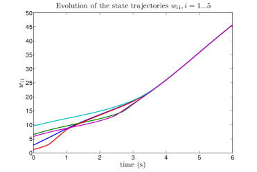
(a) The plot of $w_{i1}$, $i=1,\ldots 5$

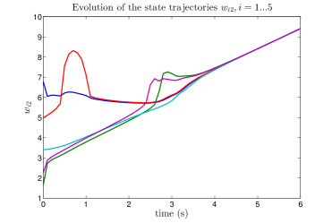
(b) The plot of $w_{i2}$, $i=1,\ldots 5$

Figure 1: Numerical simulation results of the interconnected five agents as considered in Example 1. The left-figure shows the trajectories of the first state variable of each agent, $w_{i1},i=1\ldots 5$ while the right-figure shows those of the second state variable of each agent $w_{i2},i=1\ldots 5$. The simulation results show that the proposed contraction-based distributed control law is able to synchronize the states $w_{i}$, $i=1\ldots 5$.

As in the context of the observer design given in [27], a global result can be obtained by imposing a further constraint on $P$. Specifically, the notion we need to introduce is the following.

Definition 2 (Totally Geodesically Set).

Given a $C^{2}$ function $P$ defined on ${\mathbb{R}}^{n}$ the values of which are symmetric positive definite matrices, a $C^{1}$ function $\varphi:{\mathbb{R}}^{n}\rightarrow{\mathbb{R}}_{+}$ and a real number $\bar{\varphi}$, the (level) set $S=\{x\in{\mathbb{R}}^{n},\varphi(x)=\bar{\varphi}\}$ is said to be totally geodesic with respect to $P$ if, for any $(x,v)$ in $S\times{\mathbb{R}}^{n}$ such that

$$\frac{\partial\varphi}{\partial x}(x)v=0,v^{\prime}P(x)v=1\ ,$$

any geodesic $\gamma$, i.e. a solution of
$\displaystyle\frac{d}{ds}\left(\frac{d\gamma^{*}}{ds}(s)^{\prime}P(\gamma^{*}(s))\right)l$ $(58)$
$\displaystyle\;=\;\frac{1}{2}\frac{\partial}{\partial x}\left.\left(\frac{d\gamma^{*}}{ds}(s)^{\prime}P(x)\frac{d\gamma^{*}}{ds}(s)\right)\right|_{x=\gamma^{*}(s)}\ ,$
with $\gamma(0)=x$ and $\frac{d\gamma}{ds}(0)=v$ satisfies

$$\frac{\partial\varphi}{\partial x}(\gamma(s))\frac{d\gamma}{ds}(s)=0\ ,\forall s\ .$$

For the case of two agents only, we have the following.

Proposition 7 (Global sufficient condition for $m=2$).

Assume

• there exist a $C^{3}$ function $U:{\mathbb{R}}^{n}\to{\mathbb{R}}$ which has bounded first and second derivatives, and a $C^{1}$ function $\alpha:{\mathbb{R}}^{n}\to{\mathbb{R}}^{p}$ such that, for all $x$ in ${\mathbb{R}}^{n}$, (54) is satisfied;

• there exist a positive real number $\lambda$, a $C^{3}$ function ${P}:{\mathbb{R}}^{n}\rightarrow{\mathbb{R}}^{n\times n}$ and positive real numbers $\underline{p}$ and $\overline{p}$, such that inequalities (19) hold and we have, for all $(x,v)$ in ${\mathbb{R}}^{n}\times{\mathbb{R}}^{n}$ such that $\frac{\partial U}{\partial x}(x)^{\prime}v=0$

  $$\hskip-10.00002pt\frac{1}{2}\,v^{\prime}{\mathfrak{d}}_{f}{P}(x)v+v^{\prime}{P}(x)\frac{\partial f}{\partial x}(x)v\leq-\,\lambda\,v^{\prime}P(x)v\ ,$$ (59)

• For all $\bar{U}$ in ${\mathbb{R}}$, the set $S=\{x\in{\mathbb{R}}^{n},U(x)=\bar{U}\}$ is totally geodesic with respect to $P$.

Then there exists a function ${\ell}:{\mathbb{R}}^{2n}\rightarrow{\mathbb{R}}_{+}$, invariant by permutation such that, with the controls given by

$$\phi_{i}(w)={\ell}(w)\alpha(w_{i})\,(U(w_{j})-U(w_{i}))\ ,$$

with $(i,j)\in\{(1,2),(2,1)\}$ the following holds and for all $w$ in ${\mathbb{R}}^{2n}$,

$$|W(w,t)|_{\mathcal{D}}\leq k|w|_{\mathcal{D}}\exp\left(-\frac{\lambda}{2}t\right)\ ,$$ (60)

where $t$ is any positive real number in the time domain of definition of the closed loop solution.

The proof of this result is given in Appendix .4. It borrows some ideas of [27]. However, different from [27], we have here a global convergence result. This follows from the fact that in the high gain parameter ${\ell}$, the norm of the full state space can be used (and not only the norm of the estimate as in the observer case ).

Note that nothing is said about the domain of existence of the solution.

4 Conclusion

We have studied the relationship between the exponential stability of an invariant manifold and the existence of a Riemannian metric for which the flow is “transversally” contracting. It was shown that the following properties are equivalent

1. A manifold is “transversally” exponentially stable;

2. The “transverse” linearization along any solution in the manifold is exponentially stable;

3. There exists a field of positive definite quadratic forms whose restrictions to the transverse direction to the manifold are decreasing along the flow.

As an illustrative example for these equivalence results, we have revisited the property of exponential incremental stability where we can obtain a global result.

The characterization of transverse exponential stability has allowed us to investigate a necessary condition for two different control problems of nonlinear observer design and of synchronization of nonlinear multi-agent systems which leads to a novel constructive design for each problem. Recent result by others has also shown the applicability of our results beyond these two control problems. Although the main results hold for local uniform transverse exponential stability, we show that global results can also be obtained in some particular cases. The extension of all the results to the global case is currently under study.

References

- [1] V. Andrieu, G. Besancon, and U. Serres. Observability necessary conditions for the existence of observers. In Proc. of the 52nd IEEE Conference on Decision and Control, 2013.
- [2] V. Andrieu, B. Jayawardhana, and L. Praly. On the transverse exponential stability and its use in incremental stability, observer and synchronization. In Proc. of the 52nd IEEE Conference on Decision and Control, 2013.
- [3] V. Andrieu and L. Praly. On the existence of Kazantzis-Kravaris / Luenberger Observers. SIAM Journal on Control and Optimization, 45(2):432–456, 2006.
- [4] D. Angeli. A Lyapunov approach to incremental stability properties. Automatic Control, IEEE Transactions on, 47(3):410–421, 2002.
- [5] D. Angeli. Further results on incremental input-to-state stability. Automatic Control, IEEE Transactions on, 54(6):1386–1391, 2009.
- [6] A. Astolfi and R. Ortega. Invariance: A new tool for stabilization and adaptive control of nonlinear systems. IEEE Transactions on Automatic Control, 48(4):590–606, 2003.
- [7] H. Brezis. Opérateur maximaux monotones et semi-groupes de contractions dans les espaces de Hilbert, volume 5. Mathematics Studies, 1973.
- [8] C. De Persis and B. Jayawardhana. On the internal model principle in the coordination of nonlinear systems. IEEE Transactions on Control of Network Systems, 2014.
- [9] B. P. Demidovich. Dissipativity of a system of nonlinear differential equations in the large. Uspekhi Matematicheskikh Nauk, 16(3):216–216, 1961.
- [10] A.F. Filippov. Differential Equations with Discontinuous Right Hand Sides. Mathematics and Its Applications. Kluwer Academic Publishers, 1988.
- [11] F. Forni and R. Sepulchre. A differential Lyapunov framework for contraction analysis. Automatic Control, IEEE Transactions on, 59(3):614–628, March 2014.
- [12] V. Fromion and G. Scorletti. Connecting nonlinear incremental Lyapunov stability with the linearizations Lyapunov stability. In Decision and Control, 2005 and 2005 European Control Conference. CDC-ECC’05. 44th IEEE Conference on, pages 4736–4741. IEEE, 2005.
- [13] P. Hartman. Ordinary differential equations. Wiley, 1964.
- [14] MW Hirsch, C Pugh, and M Shub. Invariant manifolds, volume 583 of Lecture notes in mathematics. Springer, 1977.
- [15] George Isac and Sándor Zoltán Németh. Scalar and asymptotic scalar derivatives: theory and applications, volume 13. Springer, 2008.
- [16] Alberto Isidori and Christopher I Byrnes. Output regulation of nonlinear systems. Automatic Control, IEEE Transactions on, 35(2):131–140, 1990.
- [17] Jérôme Jouffroy. Some ancestors of contraction analysis. In Decision and Control, 2005 and 2005 European Control Conference. CDC-ECC’05. 44th IEEE Conference on, pages 5450–5455. IEEE, 2005.
- [18] DC Lewis. Metric properties of differential equations. American Journal of Mathematics, 71(2):294–312, 1949.
- [19] DC Lewis. Differential equations referred to a variable metric. American Journal of Mathematics, 73(1):48–58, 1951.
- [20] W. Lohmiller and J.-J. E Slotine. On contraction analysis for non-linear systems. Automatica, 34(6):683–696, 1998.
- [21] S.Z. Németh. Geometric aspects of Minty-Browder monotonicity. PhD thesis, PhD thesis, E ötvös Loránd University. Budapest, 1998.
- [22] A Pavlov, A Pogromsky, Nathan van de Wouw, and Henk Nijmeijer. Convergent dynamics, a tribute to Boris Pavlovich Demidovich. Systems & Control Letters, 52(3):257–261, 2004.
- [23] A. Pavlov, N. van de Wouw, and H. Nijmeijer. Uniform Output Regulation of Nonlinear Systems: A convergent Dynamics Approach. Birkhauser, 2005.
- [24] Simeon Reich. Nonlinear semigroups, fixed points, and geometry of domains in Banach spaces. Imperial College Press, 2005.
- [25] B. S. Rüffer, N. van de Wouw, and M. Mueller. Convergent systems vs. incremental stability. Systems & Control Letters, 62(3):277–285, 2013.
- [26] T. Sakai. Riemaniann Geometry, volume 149 of Translation of Mathematical Monographs. American Mathematical Society, 1996.
- [27] R.G. Sanfelice and L. Praly. Convergence of nonlinear observers on with a Riemannian metric (part i). Automatic Control, IEEE Transactions on, 57(7):1709–1722, 2012.
- [28] R.G. Sanfelice and L. Praly. Convergence of nonlinear observers on with a Riemannian metric (part ii). Internal report, 2013.
- [29] Luca Scardovi and Rodolphe Sepulchre. Synchronization in networks of identical linear systems. Automatica, 45(11):2557–2562, 2009.
- [30] E.D. Sontag. Contractive systems with inputs. In Perspectives in Mathematical System Theory, Control, and Signal Processing, pages 217–228. Springer, 2010.
- [31] M. Spivak. A Comprehensive Introduction to Differential Geometry, volume 2. Publish or Perish, Inc., second edition, 1979.
- [32] A.R. Teel and L. Praly. A smooth Lyapunov function from a class-$ mathcal KL$ estimate involving two positive semidefinite functions. ESAIM: Control Optim. Calc. Var., 5:313–367, 2000.
- [33] L. Wang, R. Ortega, and H. Su. On Parameter Convergence of Nonlinearly Parameterized Adaptive Systems: Analysis via Contraction and First Lyapunov’s Methods. In Proc. 53rd IEEE Conference on Decision and Control, 2014.
- [34] Peter Wieland, Rodolphe Sepulchre, and Frank Allgöwer. An internal model principle is necessary and sufficient for linear output synchronization. Automatica, 47(5):1068–1074, 2011.
- [35] T. Yoshizawa. Stability theory by Liapunov’s second method, volume 9. Mathematical Society of Japan, 1966.
- [36] Taro Yoshizawa. Extreme stability and almost periodic solutions of functional-differential equations. Archive for Rational Mechanics and Analysis, 17(2):148–170, 1964.