Thermodynamics of amyloid formation and the role of intersheet interactions

Abstract

The self-assembly of proteins into $\beta$-sheet-rich amyloid fibrils has been observed to occur with sigmoidal kinetics, indicating that the system initially is trapped in a metastable state. Here, we use a minimal lattice-based model to explore the thermodynamic forces driving amyloid formation in a finite canonical ($NVT$) system. By means of generalized-ensemble Monte Carlo techniques and a semi-analytical method, the thermodynamic properties of this model are investigated for different sets of intersheet interaction parameters. When the interactions support lateral growth into multi-layered fibrillar structures, an evaporation/condensation transition is observed, between a supersaturated solution state and a thermodynamically distinct state where small and large fibril-like species exist in equilibrium. Intermediate-size aggregates are statistically suppressed. These properties do not hold if aggregate growth is one-dimensional.

I Introduction

The formation of amyloid fibrils is currently an intensely studied phenomenon.Chiti:06 ; Knowles:11 ; Hard:14 Protein aggregates of this type are found in pathological deposits in several human diseases, but also with functional roles. In addition, they possess interesting mechanical properties, stemming from their characteristic ordered cross-$\beta$ organization. Insight into the mechanisms of amyloid formation has been gained from kinetic profiles, as measured primarily by using thioflavin T (ThT) fluorescence.Hellstrand:10 In particular, it has been shown that kinetic data for a broad range of systems can be well described in terms of a few basic mechanisms for the nucleation and growth of fibrils, through a rate-equation approach.Knowles:09 This approach can reveal some general properties of intermediate species participating in the aggregation process, and has proven useful for related self-assembly phenomena as well.Ferrone:85 ; Flyvbjerg:96

Structure-based modeling of amyloid formation is a challenge to implement, due to the wide range of spatial and temporal scales involved. Hence, all-atom computer simulations with explicit solvent have focused on characterizing monomeric forms and early aggregation events.Straub:10 By using coarse-grained models, at various levels of resolution, it has been possible to study the formation and stability of larger assemblies Auer:08 ; Junghans:08 ; Irback:08 ; Li:08 ; LiMS:08 ; Bellesia:09 ; Lu:09 ; Wang:10 ; Auer:10 ; Kashchiev:10 ; Friedman:10 ; Rojas:10 ; Urbanc:10 ; Kim:10 ; Cheon:11 ; Linse:11 ; Baiesi:11 ; Carmichael:12 ; Bieler:12 ; Smaoui:13 ; Ni:13 ; Zheng:13 ; DiMichele:13 ; Abeln:14 ; MorrissAndrews:14 ; Saric:14 ; Assenza:14 and also get insight into the thermodynamic forces at play in amyloid formation.Zhang:09 ; Auer:11 ; Schmit:11 ; Auer:14 However, to map out the thermodynamics of amyloid formation as a function of control parameters such as temperature and concentration is computationally demanding even in simple models.

In this article, we use cluster Swendsen:87 and generalized-ensemble Berg:91 ; Hansmann:93 ; Wang:01a Monte Carlo (MC) techniques, supplemented with a semi-analytical approximation, to investigate the thermodynamics of a minimal model for amyloid formation.Irback:13 We study this model for three different choices of intersheet interaction parameters. The first choice leads to aggregates with at most two layers, and therefore an essentially 1D growth. The second choice permits aggregates with more than two layers to form, but odd-layered aggregates are energetically suppressed. This choice, inspired by evidence that the core of amyloid fibrils often has a pairwise $\beta$-sheet organization,Sawaya:07 ; Fitzpatrick:13 leads to a stepwise, quasi-2D growth. In the third and final case, odd-layered aggregates are not suppressed, which opens up for 2D growth, although slower laterally than longitudinally. Using $NVT$ ensembles ($N$ is the number of peptides, $V$ is volume, $T$ is temperature), we investigate the equilibrium properties of these three systems as a function of $T$ and the concentration $c=N/V$. In addition, we study the relaxation of the systems in MC simulations under fibril-favoring conditions, starting from random initial states.

II Methods

II.1 Model

We use a minimal model for peptide aggregation where each peptide $i$ is represented by a unit-length stick centered at a site, $\textbf{r}_{i}$, on a periodic cubic lattice with volume $V=L^{3}$.Irback:13 It is thus assumed that the internal dynamics of the peptides are fast, compared to the timescales of fibril formation, and can be averaged out. The systems studied consist of $N$ identical peptides or sticks. Two peptides cannot simultaneously occupy the same site. The orientation of a peptide is specified by two perpendicular lattice unit vectors, $\hat{\textbf{b}}_{i}$ and $\hat{\textbf{p}}_{i}$, yielding a total of 24 orientational states. The $\hat{\textbf{b}}_{i}$ vector represents the N-to-C backbone direction, whereas $\pm\hat{\textbf{p}}_{i}$ are the directions in which the peptide can form intrasheet interactions. The vectors $\pm\hat{\textbf{s}}_{i}=\pm\hat{\textbf{b}}_{i}\times\hat{\textbf{p}}_{i}$ represent sidechain directions, in which the peptide can form intersheet interactions. Throughout the article, we assume units in which the lattice spacing, the peptide mass and Boltzmann’s constant have the value one.

The interaction energy is taken to have a pairwise additive form, $E=\sum_{i<j}\epsilon_{ij}$, where $\epsilon_{ij}\leq 0$. The interaction geometry is illustrated in Fig. 1. Consider an arbitrary pair $i$ and $j$ of peptides and let $\textbf{r}_{ij}=\textbf{r}_{j}-\textbf{r}_{i}$. The peptides interact ($\epsilon_{ij}\neq 0$) only if (i) they are nearest neighbors on the lattice ($|\textbf{r}_{ij}|=1$), (ii) their backbone vectors are aligned either parallel or antiparallel to each other ($|\hat{\textbf{b}}_{i}\cdot\hat{\textbf{b}}_{j}|=1$), and (iii) $\hat{\textbf{b}}_{i}\cdot\textbf{r}_{ij}=\hat{\textbf{b}}_{j}\cdot\textbf{r}_{ij}=0$. The interaction that takes place when these conditions are met can be of one of three types, depending on the relative orientation of the peptides:

1. The interaction is of intrasheet type if both $\hat{\textbf{p}}_{i}$ and $\hat{\textbf{p}}_{j}$ equal $\pm\textbf{r}_{ij}$, and $\epsilon_{ij}$ is then given by

   $$\epsilon_{ij}=\begin{cases}-(1+a_{\text{p}})&\text{if}\ \hat{\textbf{b}}_{i}\cdot\hat{\textbf{b}}_{j}=\hat{\textbf{p}}_{i}\cdot\hat{\textbf{p}}_{j}=1\\ -(1+a_{\text{ap}})&\text{if}\ \hat{\textbf{b}}_{i}\cdot\hat{\textbf{b}}_{j}=\hat{\textbf{p}}_{i}\cdot\hat{\textbf{p}}_{j}=-1\\ -1&\text{otherwise}\end{cases}$$ (1)

   $$\begin{split}\qquad\qquad\qquad\qquad\qquad(|\textbf{r}_{ij}|=|\hat{\textbf{b}}_{i}\cdot\hat{\textbf{b}}_{j}|=1,\ \hat{\textbf{p}}_{i},\hat{\textbf{p}}_{j}=\pm\textbf{r}_{ij})\end{split}$$

   where the first two cases represent parallel and antiparallel $\beta$-sheet structure, respectively.

2. The interaction is of intersheet type if neither $\hat{\textbf{p}}_{i}$ nor $\hat{\textbf{p}}_{j}$ equals $\pm\textbf{r}_{ij}$, which implies that both $\hat{\textbf{s}}_{i}$ and $\hat{\textbf{s}}_{j}$ equal $\pm\textbf{r}_{ij}$. The $+\hat{\textbf{s}}$ and $-\hat{\textbf{s}}$ sides of a peptide, denoted by h and p, respectively, are assumed to have different interaction properties. The $+\hat{\textbf{s}}$, or h, side is taken as more sticky or hydrophobic. The pair potential is given by

   $$\epsilon_{ij}=\begin{cases}-(1+b_{\text{hh}})&\text{if}\ \hat{\textbf{s}}_{i}=-\hat{\textbf{s}}_{j}=\textbf{r}_{ij}\\ -(1+b_{\text{hp}})&\text{if}\ \hat{\textbf{s}}_{i}=\hat{\textbf{s}}_{j}\\ -(1+b_{\text{pp}})&\text{if}\ -\hat{\textbf{s}}_{i}=\hat{\textbf{s}}_{j}=\textbf{r}_{ij}\end{cases}$$ (2)

   $$\begin{split}\qquad\qquad\qquad\qquad\qquad(|\textbf{r}_{ij}|=|\hat{\textbf{b}}_{i}\cdot\hat{\textbf{b}}_{j}|=1,\ \hat{\textbf{s}}_{i},\hat{\textbf{s}}_{j}=\pm\textbf{r}_{ij})\end{split}$$

   and is assumed lowest when the two h sides face each other ($b_{\text{hh}}\geq b_{\text{hp}},b_{\text{pp}}$).

3. If the interaction is of neither of these two types ($|\textbf{r}_{ij}|=|\hat{\textbf{b}}_{i}\cdot\hat{\textbf{b}}_{j}|=1,\hat{\textbf{p}}_{i}\cdot\hat{\textbf{p}}_{j}=\hat{\textbf{s}}_{i}\cdot\hat{\textbf{s}}_{j}=0$), the pair potential is set to $\epsilon_{ij}=-1$.

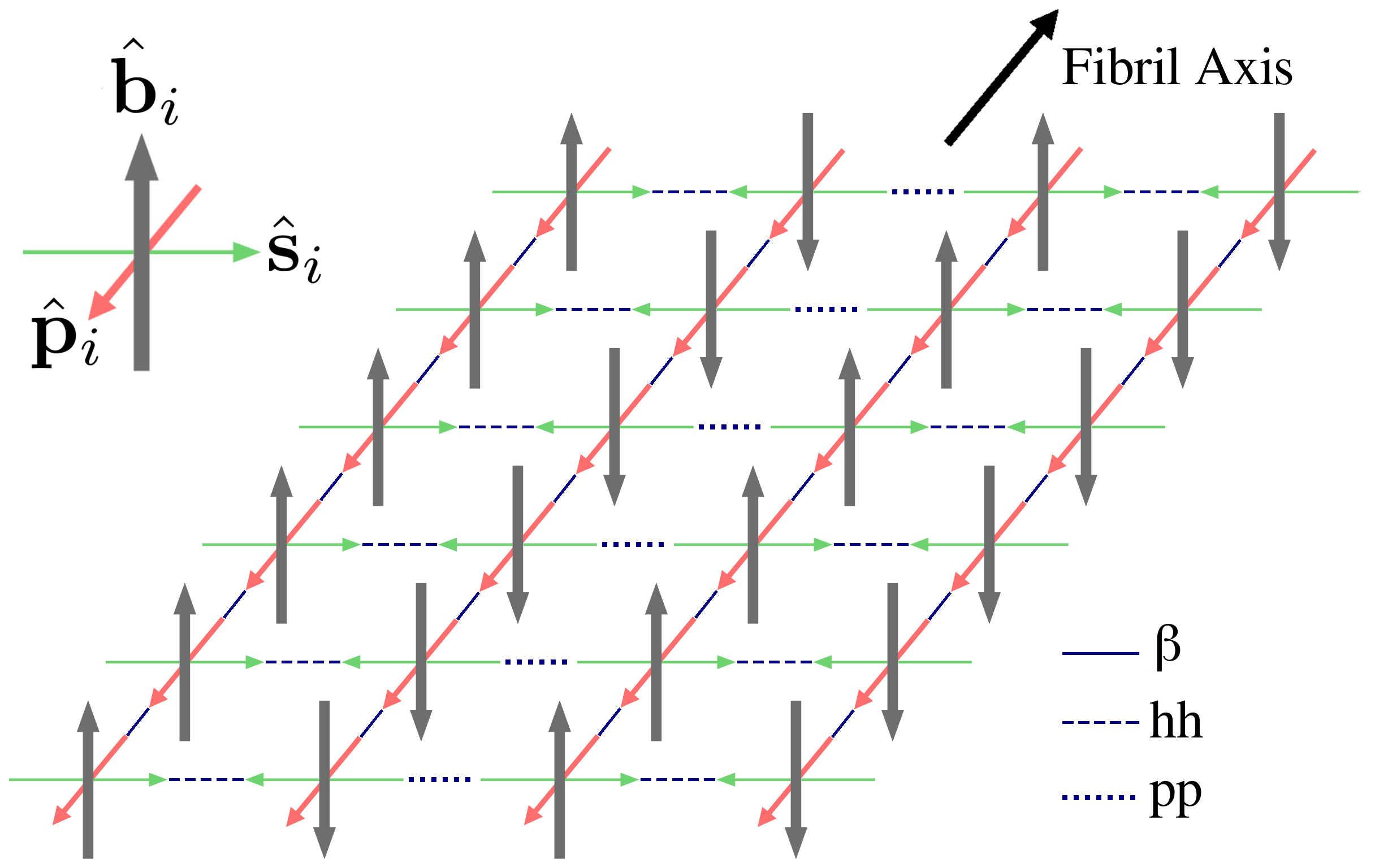
Figure 1: Example of a rectangular aggregate with length $l=6$ and width $w=4$. Along the fibril axis, the peptides are bound together by parallel $\beta$ interactions (solid blue, $\beta$). The four layers are connected either via hh interactions (blue dashes, hh), or via pp interactions (blue dots, pp). For potential B, pp interactions are weaker than hh interactions, which favors even-layered aggregates. The symmetric potential A assigns equal energy to pp, hh and hp bonds. With potential C, hp and pp interactions are missing, which makes lateral growth beyond two layers impossible.

The intersheet interactions must be weak compared to the intrasheet interactions for elongated fibril-like aggregates to form, but are nevertheless important. To assess the role played by the intersheet interactions, we study the model using three potentials A, B and C, which differ in the choice of the parameters $b_{\text{hh}}$, $b_{\text{hp}}$ and $b_{\text{pp}}$ (Table 1). The intrasheet parameters $a_{\text{p}}$ and $a_{\text{ap}}$ are the same in all three cases, namely $a_{\text{p}}=5$ and $a_{\text{ap}}=3$.

Table 1: Our three choices of the intersheet interactions parameters $b_{\text{hh}}$, $b_{\text{hp}}$ and $b_{\text{pp}}$ (Eq. 2), and the corresponding growth behavior of aggregates.

Potential	$b_{\text{hh}}$	$b_{\text{hp}}$	$b_{\text{pp}}$	Growth
A	0.5	0.5	0.5	2D
B	1	0	0	quasi-2D
C	1	$-1$	$-1$	1D

Our previous study of this model was carried out using potential B.Irback:13 With this potential, it was shown that aggregates grow in a stepwise fashion, where the major steps correspond to changes in width. Aggregate growth may here be regarded as a quasi-2D process. Potential A leads to less severe barriers to increases in width, and thereby to (asymmetric) 2D growth. With potential C, there is no interaction at all ($\epsilon_{ij}=0$) at hp and pp interfaces, which prevents the formation of aggregates with more than two stacked sheets. In this case, aggregate growth becomes an effectively 1D process.

In our model, aggregates can be assigned a length and a width, whereas growth in a third dimension does not occur due to the interaction geometry. The length $l$ and width $w$ can be conveniently defined via the inertia tensor. Specifically, we define $l=\sqrt{12\lambda_{1}^{2}/m+1}$ and $w=\sqrt{12\lambda_{2}^{2}/m+1}$, where $\lambda_{1}\geq\lambda_{2}$ are eigenvalues of this tensor and $m$ is the number of peptides in the aggregate. This definition is such that a rectangular aggregate consisting of $w$ stacked sheets with $l$ peptides each ($l\geq w$) is assigned exactly length $l$ and width $w$.

II.2 MC simulations

In order to determine the thermodynamics of these systems, one needs simulations in which large aggregates form and dissolve many times, which is challenging to achieve even in a simple model. For our thermodynamic simulations, we therefore use a Swendsen-Wang–type cluster move Swendsen:87 and a flat-histogram procedure.Berg:91 ; Hansmann:93 ; Wang:01a ; Jonsson:11

The cluster move is based on a stochastic cluster construction scheme.Swendsen:87 The procedure is recursive and begins by picking a random first cluster member, $i$. Then, all peptides $j$ interacting with peptide $i$ ($\epsilon_{ij}<0$) are identified and added to the cluster with probability $P_{ij}=1-\text{e}^{\beta\epsilon_{ij}}$, where $\beta$ is inverse temperature. This step is iterated until there are no more peptides to be tested for inclusion in the growing cluster. The resulting cluster is subject to a trial rigid-body translation or rotation, which is accepted whenever it does not cause any steric clashes. Unlike simpler cluster moves, this update can split and merge aggregates. The update fulfills detailed balance with respect to the canonical microstate distribution, $P_{\nu}\propto\text{e}^{-\beta E_{\nu}}$.

To further enhance the sampling, we use the multicanonical method,Berg:91 ; Hansmann:93 ; Wang:01a which can be very useful for systems with multimodal energy landscapes. Our simulation procedure consists of three steps.Jonsson:11 First, we estimate the density of states, $g(E)$, by the Wang-Landau method Wang:01a (an early variant of which was proposed in Ref. (48)). Second, keeping this estimate, $\tilde{g}(E)$, fixed, we simulate the ensemble $P_{\nu}\propto 1/\tilde{g}(E_{\nu})$, whose energy distribution is approximately flat.Berg:91 Finally, we calculate canonical averages via reweighting to the desired temperature.Ferrenberg:89 Throughout these simulations, we restrict the sampling to energies above a cutoff $E_{\text{min}}$. This cutoff is taken sufficiently high to avoid sampling of states containing unphysical cyclic aggregates, but sufficiently low to permit unbiased studies over the temperature range of interest. A more advanced, diffusion-optimized generalized-ensemble method was recently tested on this model.Tian:14 For our present purposes, the speed-up brought by the flat-histogram method suffices.

In our flat-histogram simulations, we use both single-peptide moves and the cluster move. The cluster move, as defined above, does not satisfy detailed balance with respect to $P_{\nu}\propto 1/\tilde{g}(E_{\nu})$. This can be easily rectified by adding a Metropolis accept/reject step with the acceptance probability given by $P_{\text{acc}}(\nu\to\nu^{\prime})=\min[1,g(E_{\nu})\text{e}^{-\beta E_{\nu}}/g(E_{\nu^{\prime}})\text{e}^{-\beta E_{\nu^{\prime}}}]$. Note that, in this context, $\beta$ is a tunable algorithm parameter, entering in the cluster construction, rather than a physical parameter. In our simulations, this parameter is chosen in the vicinity of the inverse fibrillation temperature.

In addition to the thermodynamic simulations, we perform relaxation simulations under fibril-favoring constant-temperature conditions. Here, motivated by experimental indications that amyloid growth occurs dominantly via monomer addition,Collins:04 we use single-peptide moves only; the elementary moves are translations by one lattice spacing and rotations of individual peptides. Since there is no need to observe transitions back and forth between states with and without large aggregates, the systems can be much larger than in the thermodynamic simulations ($\sim$$10^{5}$ rather than $\sim$$10^{2}$ peptides).

All statistical uncertainties quoted below are 1$\sigma$ errors.

II.3 Semi-analytical approximation

In this section, we present a semi-analytical method which can be used to estimate thermodynamic properties of the model for system sizes not amenable to direct simulation. Let $\xi$ denote a certain configuration of $m_{\xi}$ peptides forming an aggregate, and let $N_{\xi}$ denote the number of such aggregates in the system. Treating the $N_{\xi}$’s as independent variables, the chemical potential for aggregates with configuration $\xi$ may be defined as $\mu_{\xi}\equiv\partial F/\partial N_{\xi}$, where $F(T,V,\{N_{\xi}\})$ is a Helmholtz free energy. Imposing that the total number of peptides $\sum_{\xi}m_{\xi}N_{\xi}$ adds up to $N$, the function

$$\tilde{F}=F+\lambda\left(\sum_{\xi}m_{\xi}N_{\xi}-N\right),$$ (3)

is minimized at equilibrium. After eliminating the Lagrange multiplier $\lambda$, this leads to an equilibrium condition on the chemical potentials, namely

$$\mu_{\xi}=m_{\xi}\mu_{1},$$ (4)

where $\mu_{1}$ is the monomer chemical potential.

With a simplified grand-canonical description, the partition function for the set of aggregates with configuration $\xi$ is given by

$$\mathcal{Z}_{\xi}=\sum_{N_{\xi}=0}^{\infty}\frac{\text{e}^{\beta\mu_{\xi}N_{\xi}}}{N_{\xi}!}{Z^{(1)}_{\xi}}^{N_{\xi}}=\exp\left[gV\text{e}^{\beta(\mu_{\xi}-E_{\xi})}\right],$$ (5)

where $Z^{(1)}_{\xi}=gV\text{e}^{-\beta E_{\xi}}$ is the single-aggregate partition function, $E_{\xi}$ is the internal energy, and $g=24$ is the number of possible spatial orientations of the aggregate. This description neglects interactions between aggregates, but note that two adjacent $\xi$ aggregates correspond to one aggregate of some other type $\xi^{\prime}$. Eq. 5 implies that the $N_{\xi}$ variable is Poisson distributed with mean

$$\langle N_{\xi}\rangle=\frac{1}{\beta}\frac{\partial\log\mathcal{Z}_{\xi}}{\partial\mu_{\xi}}=gV\text{e}^{\beta(\mu_{1}m_{\xi}-E_{\xi})},$$ (6)

where Eq. 4 has been used. Given $\beta$, $V$ and $N$, the monomer chemical potential can be determined by approximating $N_{\xi}\approx\langle N_{\xi}\rangle$ and solving

$$N=\sum_{\xi}m_{\xi}N_{\xi},$$ (7)

for $\mu_{1}$. Knowing $\mu_{1}$, one can obtain the $N_{\xi}$’s from Eq. 6 and compute the total energy as

$$E=\sum_{\xi}E_{\xi}N_{\xi}\,.$$ (8)

The fibrillation temperature $T_{\text{f}}$ may be defined as the maximum of the heat capacity, and can therefore be estimated by numerically differentiating Eq. 8. This procedure for computing $T_{\text{f}}$ is fast and can be repeated for many different concentrations $c=N/V$, once the relevant aggregates $\xi$ and their energies $E_{\xi}$ are specified. Hence, it can be used to estimate the state of the system as a function of both $T$ and $c$.

The above scheme has similarities to the approach of Oosawa and Kasai,Oosawa:62 but has here been derived for more general choices of included aggregates. When applying it to the present model, we only consider rectangular aggregates with an energetically optimal internal organization. The generic index $\xi$ can therefore be replaced by the aggregate length $l$ and width $w$. This set of configurations turns out to be sufficient to obtain quite accurate estimates of $T_{\text{f}}$. To respect the finite size of the systems, we limit the sums over $l$ and $w$ to $l\leq l_{\max}=\min(N,L)$ and $w\leq w_{\max}(l)=\min\left[L,\mathrm{floor}\left(N/l\right)\right]$. For the potential C, which leads to aggregates with at most two proper sheets, we set $w_{\max}(l)=\min\left[2,\mathrm{floor}(N/l)\right]$.

The energy of an aggregate with length $l$ and width $w$, $E_{lw}$, is a sum of intra- and intersheet contributions. In the minimum energy configuration, the intrasheet energy is $-(1+a_{\text{p}})(l-1)w$, corresponding to a parallel organization of the $l$ peptides, whereas the intersheet energy depends on the parameters $b_{\text{hh}}$, $b_{\text{hp}}$ and $b_{\text{pp}}$. For the potentials A, B and C (Table 1), the respective minimum total energies are given by

$$E^{\mathrm{(A)}}_{lw} = -(1+a_{\text{p}})(l-1)w-\frac{3l(w-1)}{2}$$ (9)

$$E_{lw}^{(\mathrm{B})} = -(1+a_{\text{p}})(l-1)w-\frac{3l(w-1)}{2}-\frac{(1+(-1)^{w})l}{4}$$ (10)

$$E_{lw}^{(\mathrm{C})} = -(1+a_{\text{p}})(l-1)w-2l(w-1)\qquad(w=1,2)$$ (11)

With potential B, the minimal energy is achieved when both outer surfaces are entirely polar, which maximizes the number of favorable hh contacts. Likewise, with potential C, the energy of a two-sheet aggregate is minimal if the entire interface is of hh type.

III Results and discussion

We study both equilibrium and relaxation properties of the above model for the three choices of intersheet interaction parameters listed in Table 1, which correspond to 2D, quasi-2D and 1D growth and are referred to as A, B and C, respectively. The intrasheet interactions, which are stronger, stay the same in all three cases.

III.1 Equilibrium properties

The equilibrium properties of the model are investigated by using MC simulations and the semi-analytical approximation described in Sec. II. We first present the MC results which, unless otherwise stated, are obtained using $N=256$ and $L=64$, corresponding to a concentration of $c=0.977\times 10^{-3}$ per unit volume.

All three systems contain large fibril-like aggregates at low $T$, while being disordered at high $T$. The onset of fibril formation is accompanied by a peak in the heat capacity $C_{V}=(\langle E^{2}\rangle-\langle E\rangle^{2})/T^{2}$ (Fig. 2a). The fibrillation temperature, $T_{\text{f}}$, may therefore be defined as the maximum of $C_{V}$, and is found to be given by $T_{\text{f}}^{\text{(A)}}=0.66500\pm 0.00007$, $T_{\text{f}}^{\text{(B)}}=0.67093\pm 0.00007$ and $T_{\text{f}}^{\text{(C)}}=0.6548\pm 0.0002$ for systems A, B and C, respectively.

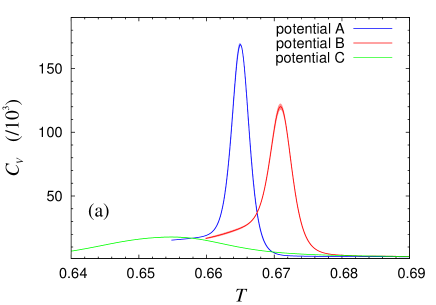
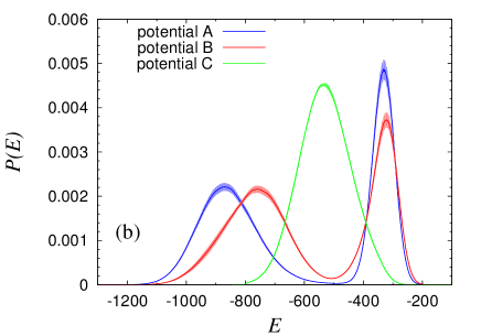
Figure 2: (a) Temperature-dependence of the heat capacity, $C_{V}$, from MC simulations with $N=256$ and $L=64$ for the potentials A, B and C (Table 1). The shaded bands indicate statistical uncertainty. Our flat-histogram simulations sample energies $E>E_{\min}$, where $E_{\min}$ is a cutoff. Data are shown only at temperatures that are sufficiently high for the effects of this cutoff to be negligible. (b) Distribution of energy, $P(E)$, at $T=T_{\text{f}}$, for the same three systems. Due to short-scale irregularities in the density of states, a moving average is used (window size $\Delta E=10$).

While $T_{\text{f}}$ is thus roughly similar for all three systems, there are large differences in the height of the $C_{V}$ peak (Fig. 2a). This fact reflects a fundamental difference between systems A and B, on one hand, and system C, on the other hand, as can be seen from the probability distribution of the total system energy $E$ (Fig. 2b). For systems A and B, with a pronounced peak in $C_{V}$, the energy distribution is clearly bimodal, showing that these systems can exist in two distinct types of states at $T=T_{\text{f}}$. The difference between the two potentials shows up in the location of the low-energy peak. For system C, the $C_{V}$ peak is broader and lower. In this system, the onset of fibril formation is smooth. As the temperature is reduced, the energy distribution slides toward lower values while retaining a unimodal shape.

The behavior of the systems at the fibrillation temperature can be further characterized in terms of the aggregate-size distribution, $p(m)$, which gives the probability for a random peptide to be part of an aggregate with size $m$ (Fig. 3a). For systems A and B, $p(m)$ is bimodal at $T=T_{\text{f}}$. Hence, whereas both small and large aggregates occur in these systems, there is a range of suppressed intermediate sizes. Above, it was seen that the energy distribution is bimodal as well (Fig. 2b). States belonging to the low-energy peak contain both small and large aggregates and contribute, therefore, to both peaks in $p(m)$, whereas high-energy states are dominated by small aggregates. Fig. 3b shows the contributions to $p(m)$ from low- and high-energy states in system B, which indeed are bi- and unimodal, respectively. Also worth noting in this figure is that the amount of aggregates with size between $m\approx 7$ and $m\approx 35$ tends to be much smaller in low-energy states than in high-energy states. Hence, the appearance of large aggregates in low-energy states occurs, at least in part, at the expense of these mid-size ones. For system C, the aggregate-size distribution $p(m)$ is fundamentally different (Fig. 3a). In this system, there is no intermediate range of suppressed sizes $m$, and therefore no clear division into either small or large species.

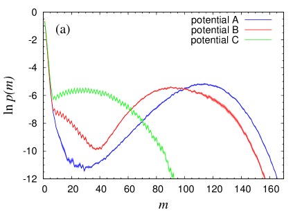
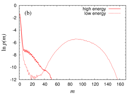
Figure 3: (a) Mass fraction of aggregates with size $m$, $p(m)$, against $m$ at $T=T_{\text{f}}$, as obtained from MC simulations with $N=256$ and $L=64$ for the potentials A, B and C (Table 1). The shaded bands indicate statistical uncertainty. The saw-tooth-like behavior that occurs for systems B and C is due to even-odd effects for two-layered aggregates. (b) Decomposition of $p(m)$ for system B into contributions from low- and high-energy states, respectively (compare Fig. 2b). Each configuration in the simulated ensemble is classified as either low energy ($E<-500$) or high energy ($E\geq-500$).

The intersheet interactions directly influence the width of the aggregates, $w$ (see Sec. II). Fig. 4 shows the mass-weighted distribution of $w$, $p(w)$, at $T=T_{\text{f}}$ for our three systems. As expected, $p(w)$ decays rapidly beyond $w=2$ for potential C, whereas potentials A and B permit the formation of wider aggregates (Fig. 4). The data also confirm that the asymmetric intersheet interactions of potential B indeed favor even-layered aggregates over odd-layered ones.

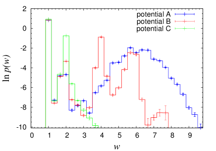
Figure 4: Mass fraction of aggregates with width $w$, $p(w)$, against $w$ at $T=T_{\text{f}}$, as obtained from MC simulations with $N=256$ and $L=64$ for the potentials A, B and C (Table 1).

The above discussion focused on results obtained using $N=256$ and $L=64$. To better understand the sharp onset of fibril formation in systems A and B, additional simulations were performed for a few different $N$, keeping the concentration approximately constant. Fig. 5a shows the specific heat, $C_{V}/N$, of system B for $N=128$, 256, 512 and 1024. As $N$ increases, the peak in $C_{V}/N$ gets sharper. However, the height of the peak increases more slowly than the linear growth expected at a first-order phase transition with a non-zero specific latent heat. Indeed, the latent heat, or energy gap, does not scale linearly with $N$ (Fig. 5b). Still, the gap grows sufficiently fast (faster than $N^{1/2}$) for the bimodality of the energy distribution to become more and more pronounced with increasing $N$ (Fig. 5b). Therefore, fibril formation sets in at a first-order-like transition, where distinct states coexist. Similar analyses were performed for potentials A and C, using $N=128$, 256 and 512. The results obtained with potential A are qualitatively similar to those just described for potential B. For potential C, $C_{V,\max}/N$ does not grow with $N$, thus confirming the conclusion that, in this case, the onset of fibril formation represents a crossover rather than a sharp transition.

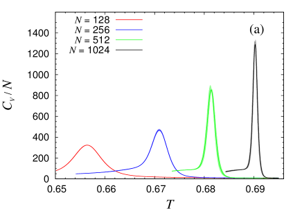
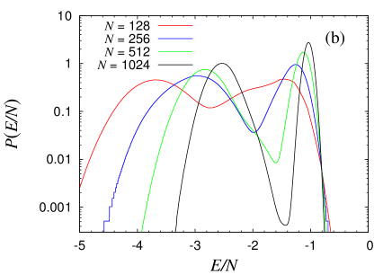
Figure 5: Finite-size scaling for system B (Table 1), at fixed concentration. The data are from MC simulations with $N=128$, 256, 512 and 1028 ($L=51$, 64, 81 and 102). (a) Temperature dependence of the specific heat, $C_{V}/N$. The shaded bands indicate statistical uncertainty. (b) Probability distribution of the energy density $E/N$ at the specific-heat maximum $T_{\text{f}}$.

Our systems resemble a lattice gas at fixed particle number, albeit with asymmetric interactions. For finite-volume liquid-vapor systems at phase coexistence, the formation of droplets due to a fixed particle excess above the ambient gas concentration has been extensively investigated,Binder:80 ; Furukawa:82 ; Biskup:02 ; Biskup:03 ; Neuhaus:03 ; Biskup:04 ; MacDowell:04 ; Nussbaumer:06 ; Nussbaumer:10 ; Bauer:10 ; Nogawa:11 often by mapping to the Ising model at fixed magnetization. A sharp transition has been shown to occur, below which the particle excess can be accommodated by gas-phase fluctuations. At the transition point, a large droplet appears, whereas intermediate-size droplets remain strongly suppressed. The volume of the droplet and the latent heat scale as $V^{3/4}$. To accurately determine the corresponding scaling behavior for our systems A and B, data over a wider range of system sizes would be required. However, the scaling of the latent heat does seem to be faster than $V^{1/2}$ and slower than $V$ (Fig. 5b).

At the droplet condensation transition, the gas concentration drops by an amount that scales as $V^{-1/4}$.Biskup:02 ; MacDowell:04 In our systems A and B, at the threshold concentration for fibril formation, $c_{\text{f}}(T)$, a similar drop occurs in the concentration of free peptides, $c_{\text{s}}$, as is illustrated in Fig. 6 by data obtained with potential B for $L=64$ and different $N$. To test the scaling with system size, this drop, $\Delta c_{\text{s}}$, was computed at the heat-capacity maxima of Fig. 5a, for system B and four different $V$. These $\Delta c_{\text{s}}$ values vary roughly as $V^{-1/4}$ with $V$ ($\Delta c_{\text{s}}\times V^{1/4}=0.0089$, 0.0079, 0.0085 and 0.0086 for $N=128$, 256, 512 and 1024, respectively).

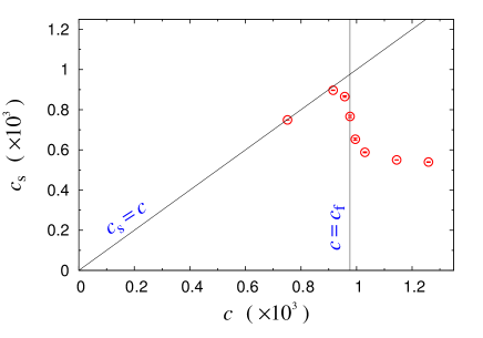
Figure 6: Concentration of free peptides, $c_{\text{s}}$, against total concentration, $c$, as obtained by MC simulations of system B (Table 1) for $T=0.67093$, $L=64$ and different $N$. At this temperature, fibrillation sets in at $c_{\text{f}}\approx 256/64^{3}$. Our definition of free peptides includes monomers and aggregates with size $m\leq 6$, so $c_{\text{s}}=c\times\sum_{m=1}^{6}p(m)$.

The results presented so far were obtained by MC simulations, which are bias-free but time-consuming. To be able to study larger systems, the approximate but much faster semi-analytical approach (Sec. II) is used. For $L=64$ and $N=256$, this method provides estimates of the fibrillation temperature ($T_{\text{f}}^{\text{(A)}}=0.6783$, $T_{\text{f}}^{\text{(B)}}=0.6866$, $T_{\text{f}}^{\text{(C)}}=0.6509$) that agree to within $\sim$1% with the MC results, and the ordering $T_{\text{f}}^{\text{(C)}}<T_{\text{f}}^{\text{(A)}}<T_{\text{f}}^{\text{(B)}}$ is correct. Having seen this agreement, the method is applied to estimate the threshold concentration, $c_{\text{f}}(T)$, as a function of temperature for the box size used in the relaxation simulations below, that is $L=512$. To this end, the fibrillation temperature is calculated for a large set of concentrations in the range $1.0\times 10^{-6}<c<2.3\times 10^{-3}$. The resulting estimates of $c_{\text{f}}(T)$ are shown in Fig. 7. The curves for systems A and B, with closely related energies (Eqs. 9,10), agree to within $\sim$1% at $T=0.65$ and become even more similar at higher $T$. For system C, our method estimates a higher $c_{\text{f}}(T)$. As discussed above, in this system, $c_{\text{f}}(T)$ represents a crossover rather than a sharp transition. The same scheme also provides an estimate of the heat capacity. It predicts $C_{V}$ to vary smoothly with $T$ in system C but that a jump occurs at $T=T_{\text{f}}$ in systems A and B, all of which match well with our earlier conclusions based on MC data for smaller systems.

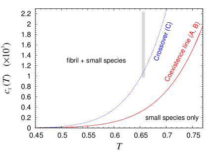
Figure 7: Temperature-dependence of the threshold concentration, $c_{\text{f}}(T)$, for systems A, B and C (Table 1), as obtained by the semi-analytical approximation (Sec. II) for $L=512$. For system C, $c_{\text{f}}(T)$ represents a crossover rather than a sharp transition. The grey vertical bar indicates the $T,c$ interval studied in our relaxation simulations.

III.2 Relaxation simulations

Having located the threshold concentration $c_{\text{f}}(T)$ for fibril formation, we next study the relaxation of the systems in constant-temperature MC simulations with $c>c_{\text{f}}(T)$, starting from random initial states. Assuming fibril growth to occur through monomer addition,Collins:04 the simulations are performed using single-peptide moves only. The parameters $T=0.6535$ and $L=512$ are the same in all these calculations, whereas $N$ varies between $2^{17}=131,072$ and 300,000. The corresponding $c$ interval is indicated in Fig. 7. To assess statistical uncertainties, a set of eight independent runs is generated for each choice of concentration and potential.

Fig. 8

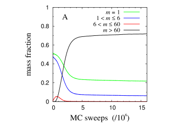
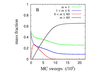
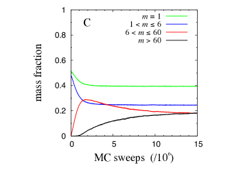
Figure 8: MC time evolution of the mass fractions of monomers ($m=1$), small aggregates ($1<m\leq 6$), mid-size aggregates ($6<m\leq 60$) and large aggregates ($m>60$) in simulations with the potentials A, B and C (Table 1), using $T=0.6535$, $L=512$ and $N=170,000$. At large times, small and large species dominate in systems A and B, whereas mid-size aggregates remain present in system C. Each MC sweep consists of $N$ single-peptide moves. The data represent averages over eight independent runs. The statistical uncertainties, indicated by shaded bands, are barely visible.

illustrates how aggregation proceeds with potentials A, B and C, by showing the evolution of the respective mass fractions of (i) monomers, (ii) small aggregates with $1<m\leq 6$ peptides, (iii) mid-size aggregates with $6<m\leq 60$, and (iv) large aggregates with $m>60$. The number of peptides is the same in all three cases ($N=170,000$). The monomer fraction is close to unity in the random initial states, but roughly a factor 2 smaller already at the time of the first measurement, due to rapid equilibration between monomers and small aggregates. After this point, the amounts of monomers and small aggregates decrease monotonically toward apparent steady-state levels. The fate of the mid-size aggregates depends on the potential. In systems A and B, these aggregates are transient species. Examples of final configurations from the simulations of these systems can be found in Fig. 9, both of which contain many large fibril-like aggregates but only very few mid-size ones. In system C, there is, by contrast, a non-negligible amount of mid-size aggregates still present in the apparent steady-state regime.

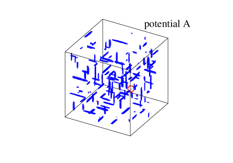
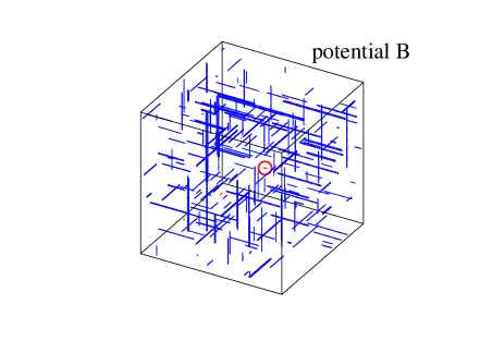
Figure 9: Final configurations from relaxation simulations with potentials A and B (Table 1), using $T=0.6535$, $L=512$ and $N=170,000$. Large ($m>60$) and mid-size ($6<m\leq 60)$ aggregates are shown in blue and red, respectively. For clarity, small species ($m\leq 6$) are not shown. At this stage, the mid-size aggregates have almost disappeared (compare Fig. 8). Red circles indicate one of $\leq$5 such aggregates in each configuration. Large aggregates tend to be shorter and wider with potential A than they are with potential B.

The apparent steady-state regimes in these simulations need not correspond to thermodynamic equilibrium states. In fact, it is likely that the true equilibrium states of the systems shown in Fig. 9 contain only one very large aggregate accompanied by surrounding small species, as observed in our equilibrium simulations of smaller systems. However, due to the very slow dynamics of large aggregates, the states shown in Fig. 9 are effectively frozen on the timescales of our simulations.

Finally, we also study how the overall rate of fibril formation scales with concentration in our relaxation simulations, focusing on systems A and B. Here, an aggregate is taken to be a fibril if its width $w$ exceeds 3.5, because thinner aggregates are unstable. This definition is somewhat arbitrary, but ambiguous assemblies close to the cutoff in width are transient species that essentially disappear as aggregation proceeds.

Fig. 10

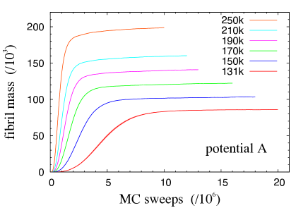
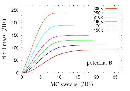
Figure 10: MC evolution of the total fibril mass in relaxation simulations with the potentials A and B (Table 1) for $T=0.6563$, $L=512$ and different $N$ between $2^{17}=131,072$ and 300,000. The data represent averages over eight independent runs, started from random initial states. The statistical uncertainties, indicated by shaded bands, are barely visible.

shows the MC evolution of the total fibril mass in systems A and B for different concentrations. The curves are sigmoidal in shape, especially at low $c$. As expected, as $c$ is increased, aggregation gets faster and the saturation level gets higher. The statistical errors are small because our systems are large. A simple measure of the overall rate of fibril formation is the time, $t_{1/2}$, at which half the saturation level is reached. In amyloid formation, the scaling of $t_{1/2}$ with $c$ has often, but not always,Meisl:14 been found to be well described by a power law, $t_{1/2}\sim c^{\gamma}$, where the exponent $\gamma\leq-0.5$ depends on both the protein and the conditions under which the fibrils grow.Knowles:09 Data for $t_{1/2}$ from our relaxation simulations do not show a perfect power-law behavior, as can be seen from a log-log plot (Fig. 11). Nevertheless, to get a measure of the overall strength of the $c$-dependence, power-law fits were performed. For system B, with quasi-2D growth, the fitted exponent, $\gamma^{\text{(B)}}=-0.8\pm 0.1$, indicates a $c$-dependence comparable in strength to that of typical experimental data.Knowles:09 For system A, with 2D growth, the $c$-dependence is slightly stronger, with a fitted exponent of $\gamma^{\text{(A)}}=-2.3\pm 0.2$.

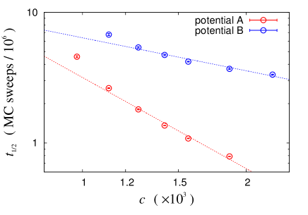
Figure 11: Concentration-dependence of the half-time for fibril formation, $t_{1/2}$, as extracted from the simulations shown in Fig. 10. The lines are power-law fits to the data, $t_{1/2}\propto c^{\gamma}$. The fitted exponents are $\gamma^{\text{(A)}}=-2.3\pm 0.2$ and $\gamma^{\text{(B)}}=-0.8\pm 0.1$ for potentials A and B, respectively.

IV Summary

Amyloid formation involves a wide range of spatial and temporal scales. In this article, we have used a minimal lattice-based model to investigate the overall thermodynamics of amyloid formation in finite systems under $NVT$ conditions. With 2D or quasi-2D aggregate growth, the model exhibits a sharp transition, from a supersaturated solution state to a distinct state where small and large species exist in equilibrium. At the threshold concentration, $c_{\text{f}}(T)$, these states coexist, thus giving rise to a bimodal energy distribution. At concentrations not too much higher than $c_{\text{f}}(T)$, there exists, therefore, a local free-energy minimum corresponding to a metastable solution state, in which the system can get trapped, thereby causing fibril formation to occur after a lag period. At and above $c_{\text{f}}(T)$, while both small and large aggregates are present, intermediate-size ones are suppressed. With 1D growth, this suppression is not observed, and the energy distribution is unimodal. Intuitively, the first-order-like transition seen with 2D or quasi-2D growth stems from a competition between bulk and surface energies. With 1D growth, this mechanism is missing, because the surface energy is associated with the fibril endpoints, whose size does not grow with fibril mass. Previous work has studied the dependence of the solubility of fibrils on their width, using different models. Zhang:09 ; Auer:10 One study compared one-, two- and three-layered aggregates, and showed that the stability region in the $T$,$c$ plane grows with increasing fibril width. Auer:10 This behavior suggests that fibril formation in a finite system may set in at a concentration roughly corresponding to the solubility of the widest aggregates that occur for this system size. Upon increasing $N$ (at fixed $c$ and $T$), one would then expect a growth in both latent heat and threshold concentration, as is indeed observed in our simulations.

The first-order-like onset of fibril formation that we observe with 2D or quasi-2D growth shows similarities with the droplet evaporation/condensation transition at liquid-vapor coexistence, which has been extensively investigated.Binder:80 ; Furukawa:82 ; Biskup:02 ; Biskup:03 ; Neuhaus:03 ; Biskup:04 ; MacDowell:04 ; Nussbaumer:06 ; Nussbaumer:10 ; Bauer:10 ; Nogawa:11 Indeed, at this transition, mid-size droplets are suppressed and the energy distribution is bimodal. Furthermore, the specific latent heat, which we find to decrease with system size (Fig. 5b), is known to vanish at the droplet transition in the limit of infinite system size.

Our equilibrium findings may be used to rationalize, in part, properties observed in our relaxation simulations. For the systems studied here, with $>$$10^{5}$ peptides, the MC evolution of the total fibril mass turns out to be highly reproducible from run to run. The trajectories are, at not too high concentrations, sigmoidal, with an initial lag phase (Fig. 10). Due to slow dynamics of large aggregates, the apparent steady-state levels at the end of the runs need not correspond to equilibrium states. However, as at equilibrium, intermediate-size aggregates are suppressed in the final states (Fig. 8), which is in line with experimental findings. Walsh:97 . With the droplet interpretation, this statistical suppression occurs because intermediate-size aggregates correspond to a free-energy maximum, at which the bulk free energy and surface energy terms balance each other. The precise shape of the aggregate-size distribution is influenced by factors that are unlikely to be captured by our simple model, such as the existence of specific oligomeric states with enhanced stability. One type of aggregate that does not occur in our simulations, due to the model geometry, is closed $\beta$-barrels, which have a potentially high stability for their size. Irback:08

- (1) F. Chiti and C. M. Dobson, Annu. Rev. Biochem. 75, 333 (2006).
- (2) T. P. J. Knowles and M. J. Buehler, Nat. Nanotechnol. 6, 469 (2011).
- (3) T. Härd, J. Phys. Chem. Lett. 5, 607 (2014).
- (4) E. Hellstrand, B. Boland, D. M. Walsh, and S. Linse, ACS Chem. Neurosci. 1, 13 (2010).
- (5) T. P. J. Knowles, C. A. Waudby, G. L. Devlin, S. I. A. Cohen, A. Aguzzi, M. Vendruscolo, E. M. Terentjev, M. E. Welland, and C. M. Dobson, Science 326, 1533 (2009).
- (6) F. A. Ferrone, J. Hofrichter, and W. Eaton, J. Mol. Biol. 183, 611 (1985).
- (7) H. Flyvbjerg, E. Jobs, and S. Leibler, Proc. Natl. Acad. Sci. USA 93, 5975 (1996).
- (8) J. E. Straub and D. Thirumalai, Curr. Opin. Struct. Biol. 20, 187 (2010).
- (9) S. Auer, C. M. Dobson, M. Vendruscolo, and A. Maritan, Phys. Rev. Lett. 101, 258101 (2008).
- (10) C. Junghans, M. Bachmann, and W. Janke, J. Chem. Phys. 128, 085103 (2008).
- (11) A. Irbäck and S. Mitternacht, Proteins 71, 207 (2008).
- (12) D. Li, S. Mohanty, A. Irbäck, and S. Huo, PLoS Comput. Biol. 4, e1000238 (2008).
- (13) M. S. Li, D. K. Klimov, J. E. Straub, and D. Thirumalai, J. Chem. Phys. 129, 175101 (2008).
- (14) G. Bellesia and J.-E. Shea, J. Chem. Phys. 130, 145103 (2009).
- (15) Y. Lu, P. Derreumaux, Z. Guo, N. Mousseau, and G. Wei, Proteins 75, 954 (2009).
- (16) Y. Wang and G. A. Voth, J. Phys. Chem. B 114, 8735 (2010).
- (17) S. Auer and D. Kashchiev, Phys. Rev. Lett. 104, 168105 (2010).
- (18) D. Kashchiev and S. Auer, J. Chem. Phys. 132, 215101 (2010).
- (19) R. Friedman, R. Pellarin, and A. Caflisch, J. Phys. Chem. Lett. 1, 471 (2010).
- (20) A. Rojas, A. Liwo, D. Browne, and H. A. Scheraga, J. Mol. Biol. 404, 537 (2010).
- (21) B. Urbanc, M. Betnel, L. Cruz, G. Bitan, and D. B. Teplow, J. Am. Chem. Soc. 132, 4266 (2010).
- (22) S. Kim, T. Takeda, and D. K. Klimov, Biophys. J. 99, 1949 (2010).
- (23) M. Cheon, I. Chang, and C. K. Hall, Biophys. J. 101, 2493 (2011).
- (24) B. Linse and S. Linse, Mol. BioSyst. 7, 2296 (2011).
- (25) M. Baiesi, F. Seno, and A. Trovato, Proteins 79, 3067 (2011).
- (26) S. P. Carmichael and M. S. Shell, J. Phys. Chem. B 116, 8383 (2012).
- (27) N. S. Bieler, T. P. J. Knowles, D. Frenkel, and R. Vácha, PLoS Comput. Biol. 8, e1002692 (2012).
- (28) M. R. Smaoui, F. Poitevin, M. Delarue, P. Koehl, H. Orland, and J. Waldispühl, Biophys. J. 104, 683 (2013).
- (29) R. Ni, S. Abeln, M. Schor, M. A. Cohen Stuart, and P. G. Bolhuis, Phys. Rev. Lett. 111, 058101 (2013).
- (30) W. Zheng, N. P. Schafer, and P. G. Wolynes, Proc. Natl. Acad. Sci. USA 110, 20515 (2013).
- (31) L. Di Michele, E. Eiser, and V. Foderà, J. Phys. Chem. Lett. 4, 3158 (2013).
- (32) S. Abeln, M. Vendruscolo, C. M. Dobson, and D. Frenkel, PLoS One 9, e85185 (2014).
- (33) A. Morriss-Andrews and J.-E. Shea, J. Phys. Chem. Lett. 5, 1899 (2014).
- (34) A. Šarić, Y. C. Chebaro, T. P. J. Knowles, and D. Frenkel, Proc. Natl. Acad. Sci. USA 111, 17869 (2014).
- (35) S. Assenza, J. Adamcik, R. Mezzenga, and P. De Los Rios, Phys. Rev. Lett. 113, 268103 (2014).
- (36) J. Zhang and M. Muthukumar, J. Chem. Phys. 130, 035102 (2009).
- (37) S. Auer, J. Chem. Phys. 135, 175103 (2011).
- (38) J. D. Schmit, K. Ghosh, and K. Dill, Biophys. J. 100, 450 (2011).
- (39) S. Auer, J. Phys. Chem. B 118, 5289 (2014).
- (40) R. H. Swendsen and J.-S. Wang, Phys. Rev. Lett. 58, 86 (1987).
- (41) B. A. Berg and T. Neuhaus, Phys. Lett. B 267, 249 (1991).
- (42) U. H. E. Hansmann and Y. Okamoto, J. Comput. Chem. 14, 1333 (1993).
- (43) F. Wang and D. P. Landau, Phys. Rev. Lett. 86, 2050 (2001).
- (44) A. Irbäck, S. Æ. Jónsson, N. Linnemann, B. Linse, and S. Wallin, Phys. Rev. Lett. 110, 058101 (2013).
- (45) M. R. Sawaya, S. Sambashivan, R. Nelson, M. I. Ivanova, S. A. Sievers, M. I. Apostol, M. J. Thompson, M. Balbirnie, J. J. W. Wiltzius, H. T. McFarlane, A. Ø. Madsen, C. Riekel, and D. Eisenberg, Nature 447, 453 (2007).
- (46) A. W. P. Fitzpatrick, G. T. Debelouchina, M. J. Bayro, D. K. Clare, M. A. Caporini, V. S. Bajaj, C. P. Jaroniec, L. Wang, V. Ladizhansky, S. A. Müller, C. E. MacPhee, C. A. Waudby, H. R. Mott, A. De Simone, T. P. J. Knowles, H. R. Saibil, M. Vendruscolo, E. V. Orlova, R. G. Griffin, and C. M. Dobson, Proc. Natl. Acad. Sci. USA 110, 5468 (2013).
- (47) S. Æ. Jónsson, S. Mohanty, and A. Irbäck, J. Chem. Phys. 135, 125102 (2011).
- (48) O. Engkvist and G. Karlström, Chem. Phys. 213, 63 (1996).
- (49) A. M. Ferrenberg and R. H. Swendsen, Phys. Rev. Lett. 63, 1195 (1989).
- (50) P. Tian, S. Æ. Jónsson, J. Ferkinghoff-Borg, S. V. Krivov, K. Lindorff-Larsen, A. Irbäck, and W. Boomsma, J. Chem. Theory Comput. 10, 543 (2014).
- (51) S. R. Collins, A. Douglass, R. D. Vale, and J. S. Weissman, PLoS Biol. 2, e321 (2004).
- (52) F. Oosawa and M. Kasai, J. Mol. Biol. 4, 10 (1962).
- (53) K. Binder and M. H. Kalos, J. Stat. Phys. 22, 363 (1980).
- (54) H. Furukawa and K. Binder, Phys. Rev. A 26, 556 (1982).
- (55) M. Biskup, L. Chayes, and R. Kotecký, EPL 60, 21 (2002).
- (56) M. Biskup, L. Chayes, and R. Kotecký, Commun. Math. Phys. 242, 137 (2003).
- (57) T. Neuhaus and J. S. Hager, J. Stat. Phys. 113, 47 (2003).
- (58) M. Biskup, L. Chayes, and R. Kotecký, J. Stat. Phys. 116, 175 (2004).
- (59) L. G. MacDowell, P. Virnau, M. Müller, and K. Binder, J. Chem. Phys. 120, 5293 (2004).
- (60) A. Nußbaumer, E. Bittner, T. Neuhaus, and W. Janke, EPL 75, 716 (2006).
- (61) A. Nußbaumer, E. Bittner, and W. Janke, Prog. Theor. Phys. Suppl. 184, 400 (2010).
- (62) B. Bauer, E. Gull, S. Trebst, M. Troyer, and D. A. Huse, J. Stat. Mech., P01020(2010).
- (63) T. Nogawa, N. Ito, and H. Watanabe, Phys. Rev. E 84, 061107 (2011).
- (64) G. Meisl, X. Yang, E. Hellstrand, B. Frohm, J. B. Kirkegaard, S. Cohen, C. M. Dobson, S. Linse, and T. P. J. Knowles, Proc. Natl. Acad. Sci. USA 111, 9384 (2014).
- (65) D. M. Walsh, A. Lomakin, G. B. Benedek, M. M. Condron, and D. B. Teplow, J. Biol. Chem. 272, 22364 (1997).