Solitons in an effective theory of CP violation

Abstract

We study an effective field theory describing CP-violation in a scalar meson sector. We write the simplest interaction that we can imagine,

$${\cal L}\sim\epsilon_{i_{1}\cdots i_{5}}\epsilon^{\mu_{1}\cdots\mu_{4}}\phi_{i_{1}}\partial_{\mu_{1}}\phi_{i_{2}}\partial_{\mu_{2}}\phi_{i_{3}}\partial_{\mu_{3}}\phi_{i_{4}}\partial_{\mu_{4}}\phi_{i_{5}}$$

which involves 5 scalar fields. The theory describes CP-violation only when it contains scalar fields representing mesons such as the $K^{*}_{0}$, sigma, $f_{0}$ or $a_{0}$. If the fields represent pseudo-scalar mesons, such as B, K and $\pi$ mesons then the Lagrangian describes anomalous processes such as $KK\to\pi\pi\pi$. We speculate that the field theory contains long lived excitations corresponding to $Q$-ball type domain walls expanding through space-time. In an 1+1 dimensional, analogous, field theory we find an exact, analytic solution corresponding to such solitons. The solitons have a U(1) charge $Q$, which can be arbitrarily high, but oddly, the energy behaves as $Q^{2/3}$ for large charge, thus the configurations are stable under disintegration into elementary charged particles of mass $m$ with $Q=1$. We also find analytic complex instanton solutions which have finite, positive Euclidean action.

I Introduction

CP violation is predicted by the standard model Burgess and Moore (2006), and exists because of the Kobayashi-Maskawa mass matrix Kobayashi and Maskawa (1973) which crucially involves and mixes three flavours of quarks. However, the CP-violation in the standard model is woefully inadequate to describe the baryon asymmetry of the universe Sakharov (1967); Kuzmin (1970); Weinberg (1979). In this letter we look for new non-perturbative sources of CP violation within the context of the standard model. Solitons and instantons, classical field configurations in general, are understood to contribute to quantum amplitudes in a non-perturbative dependence on the coupling constant Coleman (1979). Here we look for solitons-like configurations in an effective theory of mesons. Such an effective theory would arise within a low energy description of the dynamics of the mesons in the standard model.

CP-violation could be modelled, in a possible effective description, by the Lagrangian containing five real scalar (not pseudo-scalar) fields $\phi_{i},i=1\cdots 5$ representing the various mesons, with a CP violating interaction term:

$${\cal L}={\textstyle{1\over 2}}\left(\partial_{\mu}\phi_{i}\partial^{\mu}\phi_{i}-m_{i}^{2}\phi_{i}^{2}\right)+{\textstyle{\lambda\over 2}}\epsilon_{i_{1}\cdots i_{5}}\epsilon^{\mu_{1}\cdots\mu_{4}}\phi_{i_{1}}\partial_{\mu_{1}}\phi_{i_{2}}\partial_{\mu_{2}}\phi_{i_{3}}\partial_{\mu_{3}}\phi_{i_{4}}\partial_{\mu_{4}}\phi_{i_{5}}$$ (1)

where a sum over repeated latin indices from $1,\cdots,5$ and a sum over repeated greek indices from $0,\cdots,3$ is understood. Such interactions have been considered before in the context of Bi and Multi Gallileon theories Padilla et al. (2011, 2010). This Lagrangian is CP violating if the fields are taken even under time reversal. Lorentz invariance implies the CPT theorem Streater and Wightman (2000), hence CP violation is the same as time reversal violation. The interaction in the Lagrangian (1) is odd under time reversal. It is easy to imagine that there are other terms in the Lagrangian that give rise to CP conserving interactions between the mesons and require the fields be time reversal even.

The pseudo-scalar B mesons decay to lighter hadronic mesons through flavour changing, charged current, weak leptonic decays that contain CP violating channels Durieux and Grossman (2015); Aaij et al. (2014); Gronau and London (1990). The decay$B\rightarrow 2\,K\,2\,\pi$, is of great specific interest in the experiment LHCb that is going on at the present time at the accelerator at CERN Alves Jr et al. (2008) . The interaction in (1) cannot describe such decays as it is not CP-violating for pseudo-scalar meson fields. However, the interaction in (1) appears as the lowest order term in the expansion of the Wess-Zumino-Novikov-Witten Wess and Zumino (1971); Witten (1983a); Novikov (1982) that must be added to the usual Skyrme Skyrme (1961, 1962); Gisiger and Paranjape (1998) model. The interaction in (1) then describes anomalous processes such as $KK\to\pi\pi\pi$ which are of course allowed in QCD but absent in the usual Skyrme model without the WZNW term Witten (1983a, b, 1979).

Consider the ansatz

$$\phi_{1}+i\phi_{2} = f(r)e^{i\omega t}$$ (2)

$$(\phi_{3},\phi_{4},\phi_{5}) = g(r)\hat{r}(\theta,\varphi)$$ (3)

with a mass $m$ for the fields $\phi_{1}$ and $\phi_{2}$, and zero mass for the remaining fields. This ansatz yields the equations of motion:

$$-\omega^{2}f-(1/r^{2})(r^{2}f^{\prime})^{\prime}+m^{2}f+60\lambda g^{\prime}g^{2}f/r^{2} = 0$$ (4)

$$-(1/r^{2})(r^{2}g^{\prime})^{\prime}+60\lambda\omega g^{\prime}gf^{2}/r^{2} = 0$$ (5)

We imagine the existence of localized, finite energy solutions to these equations of motion. The fields $f(r)$ and $g(r)$ both vanish at the origin and stay negligible until they reach a certain radius $R$. Here they exhibit non-trivial behaviour, we presume $f$ has a small, positive bump while $g(r)$ interpolates to +1, and for larger $r$, $f(r)\to 0$ while $g(r)\sim 1$, although, it could well be that both fields vanish at spatial infinity. Such a configuration could be of finite energy, and depending on what other terms might be added to the Lagrangian. Usually the non-trivial dependence of the fields $\phi_{3},\phi_{4}\phi_{5}$ at $\infty$ would correspond to infinite energy, however we speculate that this is not the case. In any case, in the cosmological context, infinite energy solitons are not prohibited Vilenkin and Shellard (2000), for example, global strings are permitted. The configurations could be stable or unstable to expansion or contraction, however, we expect the configurations to be generally long lived. In that way, they could give rise to non-perturbative contributions to CP-violating processes. The analysis of this 3+1 model will be left to a future publication.

Our intuition is gleaned from the study of an analogous 1+1 dimensional model, where surprisingly, we find exact, analytic soliton and instanton solutions. Our analysis gives plausibility to the possibility that the 3+1 dimensional model contains soliton solutions and even instantons. The 1+1 dimensional instantons have a nontrivial winding at infinity, but the action is finite, which lends credence to our impression that the analogous 3+1 dimensional solutions of finite energy, would also exist. Their higher dimensional analogs would be infinite domain wall type solitons, or closed (spherical) domain walls giving rise to spherical solitons. The existence and stability of the 3+1 dimensional configurations is not studied in this paper.

II Minkowski 1+1 dimensional model

The analog of the model (1) in 1+1 dimensions contains three real scalar fields. We will write the Lagrangian for arbitrary masses, but we will specialize when we solve the equations of motion.

II.1 Action and the Equations of Motion

We will study the equations of motion corresponding to the Lagrangian density given by

$$\mathcal{L}=\frac{1}{2}\left[(\partial_{\mu}\phi_{i})(\partial^{\mu}\phi_{i})-m_{i}^{2}\phi_{i}^{2}+\lambda\epsilon_{ijk}\epsilon^{\mu\nu}\phi_{i}(\partial_{\mu}\phi_{j})(\partial_{\nu}\phi_{k})\right]$$ (6)

where summations over repeated indices are to be understood. $\mu,\nu=0,1$ and $i,j,k=1,2,3$. The equations of motion are simply

$$\partial_{\mu}\partial^{\mu}\phi_{i}+m_{i}^{2}\phi_{i}-\frac{3}{2}\lambda\epsilon_{ijk}\epsilon^{\mu\nu}(\partial_{\mu}\phi_{j})(\partial_{\nu}\phi_{k})=0$$ (7)

for $i=1,2,3$.

II.2 Energy

The Lagrangian (6) is invariant under the time translation giving rise to energy conservation. The interaction term being linear in time derivatives, does not contribute to the Hamiltonian and consequently nor to the energy. The energy density is given by

$$\varepsilon(x)=T^{0}_{0}=\frac{1}{2}\left[\dot{\phi_{i}}\dot{\phi_{i}}+\phi^{\prime}_{i}\phi^{\prime}_{i}+m_{i}^{2}\phi_{i}^{2}\right]$$ (8)

the total energy obtained upon integration over space.

II.3 The Case $m_{1}=m=m_{2},m_{3}=0$

The equations of motion are:

$$\partial_{\mu}\partial^{\mu}\phi_{1}+m^{2}\phi_{1}-{\textstyle{3\over 2}}\lambda\epsilon_{1jk}\epsilon^{\mu\nu}(\partial_{\mu}\phi_{j})(\partial_{\nu}\phi_{k}) = 0$$ (9)

$$\partial_{\mu}\partial^{\mu}\phi_{2}+m^{2}\phi_{2}-{\textstyle{3\over 2}}\lambda\epsilon_{2jk}\epsilon^{\mu\nu}(\partial_{\mu}\phi_{j})(\partial_{\nu}\phi_{k}) = 0$$ (10)

$$\partial_{\mu}\partial^{\mu}\phi_{3}-{\textstyle{3\over 2}}\lambda\epsilon_{3jk}\epsilon^{\mu\nu}(\partial_{\mu}\phi_{j})(\partial_{\nu}\phi_{k}) = 0$$ (11)

The kinetic term and the interaction are invariant under $SO(3)$ iso-rotations, but these are explicitly, softly broken by the mass terms. In the present case, $SO(2)$ symmetry is preserved and the Lagrangian is invariant under an iso-rotation between $\phi_{1}$ and $\phi_{2}$, $\phi_{1}+i\phi_{2}\rightarrow e^{i\alpha}(\phi_{1}+i\phi_{2})$.The corresponding conserved current is given by

$$j^{\mu}=\phi_{1}(\partial^{\mu}\phi_{2})-\phi_{2}(\partial^{\mu}\phi_{1})+\lambda\epsilon^{\mu\nu}\left[(\phi_{1}^{2}+\phi_{2}^{2})(\partial_{\nu}\phi_{3})-\phi_{3}(1/2)\partial_{\nu}(\phi_{1}^{2}+\phi_{2}^{2})\right].$$ (12)

II.4 Ansatz and exact soliton

We take the ansatz

$$\phi_{1}+i\phi_{2}=f(x)e^{i\omega(t-t_{0})}\quad\quad\phi_{3}=g(x)$$ (13)

which gives the simple, equations of motion

$$(m^{2}-\omega^{2})f-f^{\prime\prime}-3\lambda\omega fg^{\prime}=0$$ (14)

and

$$-g^{\prime\prime}+3\lambda\omega ff^{\prime}=0$$ (15)

Eqn. (15) integrates trivially as

$$g^{\prime}=\frac{3}{2}\lambda\omega f^{2}-A$$ (16)

where $A$ is a constant. The energy density in terms of $f$ and $g$ becomes

$$\varepsilon(x)=\frac{1}{2}\left[f^{\prime 2}+g^{\prime 2}+(m^{2}+\omega^{2})f^{2}\right]$$ (17)

As each term is a positive definite, the finite energy condition for a solitonic solution requires $f,f^{\prime},g^{\prime}\rightarrow 0$ as $x\rightarrow\pm\infty$. This condition gives $A=0$ and we get

$$g^{\prime}=\frac{3}{2}\lambda\omega f^{2}.$$ (18)

Putting this back in (14) we get remarkably,

$$f^{\prime\prime}+\frac{9\lambda^{2}\omega^{2}}{2}f^{3}-(m^{2}-\omega^{2})f=0$$ (19)

which is just the non-linear Schrödinger equation Ablowitz and Clarkson (1991), which is trivially integrable. We can rewrite the equation as

$$f^{\prime\prime}=-\frac{dU(f)}{df}$$ (20)

with

$$U(f)=\frac{9\lambda^{2}\omega^{2}}{8}f^{4}-\frac{m^{2}-\omega^{2}}{2}f^{2}$$ (21)

As the coefficient of $f^{4}$ in $U(f)$ is always positive there are typically two types of behaviour of $U(f)$ with respect to $f$ for $m^{2}\leq\omega^{2}$ and for $m^{2}\geq\omega^{2}$. A finite energy solitonic solution must satisfy $f\rightarrow 0$ as $x\rightarrow\pm\infty$.

II.4.1 The case $(m^{2}-\omega^{2})\leq 0$

The only solution for this case is

$$f(x)=0\hskip 56.9055pt\mbox{{\rm for all }}x$$ (22)

which gives (see (18))

$$g(x)=\mbox{{\rm constant}}=g_{0}$$ (23)

a constant. Then the three fields become

$$\phi_{1}=\phi_{2}=0,\quad\quad\phi_{3}=g_{0}.$$ (24)

The energy for the above configuration is zero. Thus the above configuration represents a vacuum which is degenerate. Different vacua of the theory correspond to different values for the constant $g_{0}$. This vacuum solution does not contain any $\lambda$-contribution as the $\lambda$-term in the equations of motion vanishes identically for the above!

II.4.2 The case $(m^{2}-\omega^{2})>0$

We can actually solve Eqn. (19) exactly. Multiplying it by $f^{\prime}$ and integrating gives

$$\frac{1}{2}f^{\prime 2}+\frac{9\lambda^{2}\omega^{2}}{8}f^{4}-\frac{1}{2}(m^{2}-\omega^{2})f^{2}=\mbox{{\rm constant }}=D.$$ (25)

Again, finite energy requires that the function $f$ and $f^{\prime}$ vanish at $x\to\pm\infty$, which requires $D=0$ and we get

$$\frac{1}{2}f^{\prime 2}+\frac{9\lambda^{2}\omega^{2}}{8}f^{4}-\frac{1}{2}(m^{2}-\omega^{2})f^{2}=0.$$ (26)

This can be written as

$$dx=\frac{df}{\frac{3\lambda\omega}{2}f\sqrt{\frac{4(m^{2}-\omega^{2})}{9\lambda^{2}\omega^{2}}-f^{2}}}$$ (27)

where we allow $\omega$ to be positive or negative to allow for either sign in the square root that we have taken. Noting that $\frac{4(m^{2}-\omega^{2})}{9\lambda^{2}\omega^{2}}>0$ and integrating we get

$$x=\pm\frac{1}{\sqrt{m^{2}-\omega^{2}}}\mbox{ {\rm sech}}^{-1}\left[\frac{3\lambda\omega f}{2\sqrt{m^{2}-\omega^{2}}}\right]+x_{0}.$$ (28)

Inverting

$$f=\frac{2\sqrt{m^{2}-\omega^{2}}}{3\lambda\omega}\mbox{ {\rm sech}}\left[\sqrt{m^{2}-\omega^{2}}\left(x-x_{0}\right)\right]$$ (29)

Putting this back in (18) and integrating gives

$$g=\frac{2\sqrt{m^{2}-\omega^{2}}}{3\lambda\omega}\mbox{ {\rm tanh}}\left[\sqrt{m^{2}-\omega^{2}}\left(x-x_{0}\right)\right]+g_{0}$$ (30)

Here $g(x=x_{0})=g_{0}$. We notice that for $g_{0}=0$ we find

$$\sum_{i}\phi^{2}_{i}=\frac{4(m^{2}-\omega^{2})}{9\lambda^{2}\omega^{2}}$$ (31)

which is a constant.

II.5 Energy and charge

The energy for such solutions is easily calculated from Eqn. (17), we find

$$E=\int_{-\infty}^{\infty}dx\varepsilon(x)=\frac{8m^{2}\sqrt{m^{2}-\omega^{2}}}{9\lambda^{2}\omega^{2}}$$ (32)

it’s dependence on $\omega$ is shown in Figure (1). The energy is zero for $\omega=\pm m$ (the degenerate vacua) and increases to infinity as $\omega\rightarrow 0$.

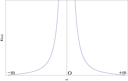
Figure 1: The behaviour of the Energy of the soliton/anti-soliton with respect to $\omega$

The charge for the above solution becomes, using the notation $f=\alpha\,{\rm sech}\beta(x-x_{0})$, and dropping $x_{0}$ due to translation invariance,

$$Q = \int dx\left(\omega f^{2}-\lambda(gff^{\prime}-f^{2}g^{\prime})\right)$$ (33)

$$= \int dx\left(\omega\alpha^{2}\,{\rm sech}^{2}\beta x-\lambda\alpha^{3}\beta(-\tanh^{2}\beta x{\rm sech}^{2}\beta x-{\rm sech}^{4}\beta x)\right)$$

$$= (\omega\alpha^{2}+\lambda\alpha^{3}\beta)\int dx\,{\rm sech}^{2}\beta x=\frac{(\omega\alpha^{2}+\lambda\alpha^{3}\beta)}{\beta}2.$$

Replacing for $\alpha$ and $\beta$ from Eqn. (29) the conserved charge becomes

$$Q=\frac{8\sqrt{m^{2}-\omega^{2}}}{9\lambda^{2}\omega}\left(1+\frac{2(m^{2}-\omega^{2})}{3\omega^{2}}\right).$$ (34)

For solitons $\omega$ and hence $Q$ is positive while for anti-solitons they are negative. We can solve for $\omega$ in terms of $m$ and $E$ from Eqn. (32),

$$\omega^{2}=\frac{-64m^{4}+\sqrt{(64m^{4})^{2}+4(64m^{6})81\lambda^{4}E^{2}}}{2\cdot 81\lambda^{4}E^{2}}.$$ (35)

For large $E$ this simplifies as

$$\omega^{2}\approx\frac{8m^{3}}{9\lambda^{2}E}\left(1+o\left(\frac{m}{E}\right)\right)$$ (36)

and then gives

$$Q=\left(\frac{1}{3}+\frac{2m^{2}}{3\omega^{2}}\right)\frac{8\sqrt{m^{2}-\omega^{2}}}{9\lambda^{2}\omega}\approx\frac{2m^{2}}{3\omega^{2}}\frac{8m}{9\lambda^{2}\omega}\left(1+o\left(\frac{\omega}{m}\right)\right)\approx 2\lambda\left(\frac{E}{2m}\right)^{3/2}$$ (37)

which shows that $E\sim m\left(\sqrt{2}Q/\lambda\right)^{2/3}$ in this limit of large $E$ and hence large $Q$. This is actually odd for a 1+1 dimensional $Q$-ball. A general anaylsis MacKenzie and Paranjape (2001) shows that the normal behaviour would be $E\sim Q^{1/2}$. The actual behaviour that we have found is normally seen in 2+1 dimensional $Q$-balls. Therefore the solitonic configuration is stable compared to $E\sim mQ$ which would be the case for $Q$ perturbative excitations of mass $m$.

For small $E$ we expand the combination

$$\frac{\sqrt{m^{2}-\omega^{2}}}{\omega}=\frac{\sqrt{m^{2}-\omega^{2}}}{\omega^{2}}\omega\approx\frac{9\lambda^{2}E}{8m^{2}}m\left(1-\frac{81\lambda^{4}E^{2}}{128m^{2}}+\cdots\right)$$ (38)

and then we can express the charge in terms of $m$ and $E$, we get

$$Q=\frac{E}{m}\left(1+\frac{1}{6}\cdot\frac{81\lambda^{4}}{64m^{2}}E^{2}\right).$$ (39)

This also gives $E<mQ$ which again seems to indicate stability, which is rather surprising, as this would indicate that the perturbative excitations are unstable to forming $Q$ balls, even for individual particles of charge $Q=1$ and mass $m$. However, at the moment, we only consider this as in indication, which needs to be verified by numerical calculations.

III Instantons

III.1 Action and Equation of Motion

The Euclidean action is obtained via the analytic continuation $t\to-i\tau$ resulting in $iS_{M}\to-S_{E}$, giving

$$S_{E}=\frac{1}{2}\,\int d^{2}x\,\left[(\partial_{\mu}\phi_{i})(\partial_{\mu}\phi_{i})\,+\,m_{i}^{2}\phi_{i}^{2}\,-\,i\lambda\epsilon_{\mu\nu}\,\epsilon_{ijk}\phi_{i}(\partial_{\mu}\phi_{j})(\partial_{\nu}\phi_{k})\right]$$ (40)

where indicies are simply written below as the Euclidean metric is the identity matrix, $g_{\mu\nu}=\delta_{\mu\nu}$. It is important to note that the interaction term remains imaginary in Euclidean space, this is an example of a complex action, and the corresponding non-trivial solutions to the equations of motion may not be real Alexanian et al. (2008). The equation of motion for field $\phi_{i}$ becomes

$$\partial_{\mu}\partial_{\mu}\phi_{i}\,-\,m_{i}^{2}\phi_{i}\,+\,\frac{3i\lambda}{2}\,\epsilon_{\mu\nu}\,\epsilon_{ijk}\,(\partial_{\mu}\phi_{j})\,(\partial_{\nu}\phi_{k})=0$$ (41)

III.2 Finite Action Solutions to Equation of Motion

Obviously, no real, non-trivial solutions exist to these equations of motion. To obtain non-trivial solutions we must complexify the fields. We could, in principle, take one field complex, or all three complex, either choice will render the equations of motion (41) real in either case. We find that taking one field complex does not lead to a non-singular solutions. Hence we take the ansatz

$$\phi_{1}(r,\theta) = i\,f(r)\,\cos{\omega\theta}$$

$$\phi_{2}(r,\theta) = i\,f(r)\,\sin{\omega\theta}$$

$$\phi_{3}(r,\theta) = i\,g(r)$$ (42)

where for periodicity, actually, $\omega=N$ for some integer $N$. To separate the $\theta$ dependence we must take $m_{1}=m_{2}=m$ and then we get the equations

$$r^{2}\,f^{\prime\prime}\,+\,r\,f^{\prime}\,-\,(m^{2}r^{2}+\omega^{2})\,f\,+\,3\omega\lambda rfg^{\prime} = 0$$ (43)

$$r^{2}\,g^{\prime\prime}\,+\,r\,g^{\prime}\,-\,m^{2}_{3}r^{2}\,g\,-\,3\omega\lambda rff^{\prime} = 0$$ (44)

where the prime on functions means differentiation with respect to $r$. Also we have suppressed the functional dependences of $f$ and $g$ on $r$. We notice that the above equations simplify significantly if we take all particles to be massless i.e. $m_{1}=m_{2}=m_{3}=0$:

$$r^{2}\,f^{\prime\prime}\,+\,r\,f^{\prime}\,-\,\omega^{2}\,f\,+\,3\omega\lambda rfg^{\prime} = 0$$ (45)

$$r^{2}\,g^{\prime\prime}\,+\,r\,g^{\prime}\,-\,3\omega\lambda rff^{\prime} = 0$$ (46)

Equation (46) integrates directly as

$$(rg^{\prime})^{\prime}=\frac{3}{2}\omega\lambda(f^{2})^{\prime}$$ (47)

which gives

$$g^{\prime} = \frac{3}{2r}\omega\lambda f^{2}\,+\,\frac{c_{1}}{r}$$ (48)

where $c_{1}$ is an arbitrary integration constant. Finite Euclidean action, after some algebra, requires $c_{1}=0$. Thus we get

$$g^{\prime}=\frac{3}{2r}\omega\lambda f^{2}.$$ (49)

Then using (49) in (46) we have

$$r^{2}\,f^{\prime\prime}\,+\,r\,f^{\prime}\,-\,\omega^{2}\,f\,+\,3\omega\lambda rf\left(\frac{3}{2r}\omega\lambda\,f^{2}\right) = 0$$

$$\Rightarrow\qquad r^{2}\,f^{\prime\prime}\,+\,r\,f^{\prime}\,-\,\omega^{2}\,f\,+\,\frac{9}{2}\omega^{2}\lambda^{2}\,f^{3} = 0$$ (50)

Multiplying (50) by $f^{\prime}$ and integrating and after some trivial algebra, gives

$$(f^{\prime})^{2}=\frac{\omega^{2}\,f^{2}}{r^{2}}\left(1\,-\,\frac{9}{2}\omega^{2}\lambda^{2}\,f^{2}\right).$$ (51)

This yields, after elementary integration,

$$f\,=\,\frac{4}{3\lambda}\,\frac{(r/r_{0})^{\pm\omega}}{\left((r/r_{0})^{\pm 2\omega}+1\right)}$$ (52)

where $r_{0}$ is effectively the integration constant. One can also check that for both $\pm\omega$ we get the same solution for $f$:

$$f = \frac{4}{3\lambda}\,\frac{1}{\left((r/r_{0})^{\omega}+(r/r_{0})^{-\omega}\right)}$$ (53)

Using (53) in (49) and integrating we get

$$g = \frac{-4}{3\lambda}\,\frac{1}{\left((r/r_{0})^{2\omega}+1\right)}\,+\,c$$ (54)

where $c$ is an integration constant. Hence the field solutions to the equations of motion can be written as

$$\phi_{1}(r,\theta) = \frac{4i}{3\lambda}\,\frac{(r/r_{0})^{\omega}}{\left((r/r_{0})^{2\omega}+1\right)}\,\cos{\omega\theta}$$

$$\phi_{2}(r,\theta) = \frac{4i}{3\lambda}\,\frac{(r/r_{0})^{\omega}}{\left((r/r_{0})^{2\omega}+1\right)}\,\sin{\omega\theta}$$

$$\phi_{3}(r,\theta) = -\,\frac{4i}{3\lambda}\,\frac{1}{\left((r/r_{0})^{2\omega}+1\right)}\,+\,ic$$ (55)

III.3 The Euclidean action for our solution

In terms of our ansatz, (42), the Euclidean action (40) becomes

$$S_{E}=-\pi\,\int^{\infty}_{0}dr\,\left[r\,\left(f^{\prime}\right)^{2}\,+\,r\,\left(g^{\prime}\right)^{2}\,+\,\frac{\omega^{2}}{r}\,f^{2}\,-\,2\omega\,\lambda\,f^{2}\,g^{\prime}\,+\,2\omega\,\lambda\,g\,f\,f^{\prime}\right]$$ (56)

We first note that the action is independent of the constant that we could add to $g$ in Eqn. (54), the terms involving $g^{\prime}$ of course do not see the constant, and the final term changes by a total derivative, which integrates to zero given the boundary conditions $f|_{r=0}=f|_{r=\infty}=0$. Then using the equations of motion for $g^{\prime}$ and for $f^{\prime}$, Eqn. (49) and Eqn. (50), we find

$$S_{E}=-\pi\,\int^{\infty}_{0}dr\,r\left(\frac{\omega^{2}}{r^{2}}\,f^{2}\,-\,\frac{9\omega^{2}\,\lambda^{2}}{2r^{2}}f^{4}\right).$$ (57)

We could substitute the solution for $f$ directly into this expression and integrate, but there is a more elegant method. We use Eqn. (51) to insert unity into the integral

$$S_{E} = -\pi\,\int^{\infty}_{0}dr\,r\left(\frac{\omega^{2}}{r^{2}}\,f^{2}\,\left(1-\,\frac{9\,\lambda^{2}}{2}f^{2}\right)\frac{f^{\prime}}{\frac{\omega f}{r}\sqrt{1-\frac{9\lambda^{2}}{4}f^{2}}}\right)$$ (58)

$$= \frac{-\pi\omega}{2}\,\int^{\infty}_{0}dr\,\left(\frac{1-\,\frac{9\,\lambda^{2}}{2}f^{2}}{\sqrt{1-\frac{9\lambda^{2}}{4}f^{2}}}\right)(f^{2})^{\prime}$$

$$= 2\times\frac{-\pi\omega}{2}\,\int^{\frac{4}{9\lambda^{2}}}_{0}dx\,\left(\frac{1-\,\frac{9\,\lambda^{2}}{2}x}{\sqrt{1-\frac{9\lambda^{2}}{4}x}}\right)$$

where we have used the fact that $x=f^{2}$ rises to its maximum value $f_{max}=\frac{4}{9\lambda^{2}}$ and then falls back down to zero, and thus we integrate only up to this value with the positive square root and multiply the result by 2. The integral is again elementary and yields

$$S_{E}=\frac{8\pi\omega}{27\lambda^{2}}.$$ (59)

IV Addition of a quartic potential

IV.1 Minkowski solution

We have observed in Eqn. (31) that

$$\sum_{i}\phi^{2}_{i}=\frac{4(m^{2}-\omega^{2})}{9\lambda^{2}\omega^{2}}.$$ (60)

Hence if we add the potential

$$V(\phi_{i})=\gamma\left(\sum_{i}\phi^{2}_{i}-\frac{4(m^{2}-\omega^{2})}{9\lambda^{2}\omega^{2}}\right)^{2}$$ (61)

to the action, its contribution to the equations of motion

$$\frac{\partial V}{\partial\phi_{i}}=2\gamma\left(\sum_{i}\phi^{2}_{i}-\frac{4(m^{2}-\omega^{2})}{9\lambda^{2}\omega^{2}}\right)2\phi_{i}$$ (62)

will exactly vanish for the solution that we have found. Thus the full potential will correspond to the spontaneous symmetry breaking potential $V(\phi)$ in addition to the explicit symmetry breaking mass terms for the fields $(m^{2}/2)\phi_{1}^{2}$ and $(m^{2}/2)\phi_{2}^{2}$. The potential $V(\phi)$ will spontaneously break the original symmetry $SO(3)\to SO(2)$, giving rise to one massive scalar with $M^{2}=\frac{8\gamma(m^{2}-\omega^{2})}{9\lambda^{2}\omega^{2}}$ and two massless scalar fields. The explicit symmetry breaking terms preserve the $SO(2)$ symmetry, however, cause the putatively massless Goldstone bosons of the spontaneous symmetry breaking to become “pseudo-Goldstone” bosons of mass $m$. For the notion that the “pseudo-Goldstone” boson fields are much lighter than the massive field, we should like to have $M>>m$, however, this is not at all required for our solutions to exist.

IV.2 Euclidean solution

We start with the observation that, the constant in Eqn. (55) for $\phi_{3}=ig$ is not at all determined, and does not affect the value of the euclidean action. If we choose $c=2/3\lambda$ we find

$$g=\frac{-2}{3\lambda}\left(\frac{1-(r/r_{0})^{2\omega}}{1+(r/r_{0})^{2\omega}}\right),$$ (63)

and then

$$\sum_{i}\phi_{i}^{2}=-(f^{2}+g^{2})=-\frac{16}{9\lambda^{2}}.$$ (64)

Therefore, if we add the potential

$$V_{E}(\phi_{i})=\gamma_{E}\left(\sum_{i}\phi_{i}^{2}+\frac{16}{9\lambda^{2}}\right)^{2}$$ (65)

as in the Minkowski case, the contribution to the equations of motion will exactly vanish. The potential added is not of the symmetry breaking type, all the fields become massive, with mass $M^{2}=4\gamma_{E}\frac{16}{9\lambda^{2}}$.

V Conclusion

We have studied a model of possible CP-violation where in the 1+1 dimensional analog, we find exact solitons of finite energy and exact instantons of finite Euclidean action. The instantons could have an interpretation as exact solitons of a 2+1 dimensional theory, although the structure of our theory requires additional fields in higher dimensions. Exact solitons in a somewhat related model, were found a long time ago by Jackiw and Pi Jackiw and Pi (1990). The Jackiw-Pi model contains a Chern-Simons term which our interaction imitates, and a quartic interaction between the Schrodinger field, which we generate when we isolate the equation for say $f$, in Eqn. (50). The energy and the action of our solutions depends, as expected, non-perturbatively on the coupling constant, hence we believe that these classical solutions will give rise to new non-perturbative contributions to CP-violation. It is not clear what tunnelling our instanton solutions describe. The instanton solutions are established for the massless, potential free theory, however, they are also valid for the theory with a standard quartic self coupling between the fields, which are degenerate in mass. There is no obvious meta-stable state whose decay is mediated by the instantons.

The Minkowski solutions are of the $Q$-ball type, and for large $Q$, they owe their stability to the fact that the energy increases much slower than linearly for large charge. Therefore they are energetically stable against disintegration into $Q$ perturbative, massive particles. Interestingly, even for small $Q$, our solitons have less energy than $Q$ perturbative, massive particles, $mQ$. We then can imagine that the perturbative excitations are not stable, and should decay into $Q$-ball type solutions. This kind of instability seems new, we are not aware of it in any other model. With the addition of the quartic potential term of the symmetry breaking type, because of the “pseudo-Goldstone” mass terms, the potential has in fact exactly two discrete, degenerate vacua, $\phi_{1}=\phi_{2}=0$, $\phi_{3}=\pm\frac{2\sqrt{m^{2}-\omega^{2}}}{3\lambda\omega}$. The fields of our $Q$-ball type soliton interpolate between the two vacua. In principle, there should exist instantons which tunnel between the two vacua, however, we find no such instantons. The instantons we find are for a modified theory which has a unique vacuum at $\phi_{i}=0$.

It would be interesting and important to generalize our results to a 3+1 dimensional model.

VI ACKNOWLEDGEMENTS

We thank Bhujyo Bhattacharya for useful discussions. We thank NSERC, Canada for financial support. The visit of NC and RH to Montréal, where this work was completed, was possible due to fellowships from the Canadian Commonwealth Scholarship, we gratefully acknowledge the assistance. This work was written up while MP was visiting Urjit Yajnik at IITBombay, Mumbai, India and the Inter-University Center for Astronomy and Astrophysics, Pune, India, their hospitality is also gratefully acknowledged.

References

• Burgess and Moore (2006) C. Burgess and G. Moore, The standard model: A primer (Cambridge University Press, 2006).
• Kobayashi and Maskawa (1973) M. Kobayashi and T. Maskawa, Progress of Theoretical Physics 49, 652 (1973).
• Sakharov (1967) A. Sakharov, Sov. Phys. JETP Lett 5, 24 (1967).
• Kuzmin (1970) V. A. Kuzmin, Pisma Zh. Eksp. Teor. Fiz. 12, 335 (1970).
• Weinberg (1979) S. Weinberg, Phys. Rev. Lett. 42, 850 (1979).
• Coleman (1979) S. R. Coleman, Subnucl. Ser. 15, 805 (1979).
• Padilla et al. (2011) A. Padilla, P. M. Saffin, and S.-Y. Zhou, Phys. Rev. D83, 045009 (2011), eprint 1008.0745.
• Padilla et al. (2010) A. Padilla, P. M. Saffin, and S.-Y. Zhou, JHEP 12, 031 (2010), eprint 1007.5424.
• Streater and Wightman (2000) R. F. Streater and A. S. Wightman, PCT, spin and statistics, and all that (Princeton University Press, 2000).
• Durieux and Grossman (2015) G. Durieux and Y. Grossman, Phys. Rev. D92, 076013 (2015), eprint 1508.03054.
• Aaij et al. (2014) R. Aaij et al. (LHCb), JHEP 10, 005 (2014), eprint 1408.1299.
• Gronau and London (1990) M. Gronau and D. London, Physical Review Letters 65, 3381 (1990).
• Alves Jr et al. (2008) A. A. Alves Jr, L. Andrade Filho, A. Barbosa, I. Bediaga, G. Cernicchiaro, G. Guerrer, H. Lima Jr, A. Machado, J. Magnin, F. Marujo, et al., Journal of instrumentation 3, S08005 (2008).
• Wess and Zumino (1971) J. Wess and B. Zumino, Physics Letters B 37, 95 (1971).
• Witten (1983a) E. Witten, Nucl. Phys. B223, 422 (1983a).
• Novikov (1982) S. P. Novikov, Usp. Mat. Nauk 37N5, 3 (1982).
• Skyrme (1961) T. H. R. Skyrme, in Proceedings of the Royal Society of London A: Mathematical, Physical and Engineering Sciences (The Royal Society, 1961), vol. 260, pp. 127–138.
• Skyrme (1962) T. H. R. Skyrme, Nuclear Physics 31, 556 (1962).
• Gisiger and Paranjape (1998) T. Gisiger and M. B. Paranjape, Physics Reports 306, 109 (1998).
• Witten (1983b) E. Witten, Nucl. Phys. B223, 433 (1983b).
• Witten (1979) E. Witten, Nuclear Physics B 160, 57 (1979).
• Vilenkin and Shellard (2000) A. Vilenkin and E. P. S. Shellard, Cosmic strings and other topological defects (Cambridge University Press, 2000).
• Ablowitz and Clarkson (1991) M. J. Ablowitz and P. A. Clarkson, Solitons, nonlinear evolution equations and inverse scattering, vol. 149 (Cambridge university press, 1991).
• MacKenzie and Paranjape (2001) R. B. MacKenzie and M. B. Paranjape, Journal of High Energy Physics 2001, 003 (2001).
• Alexanian et al. (2008) G. Alexanian, R. MacKenzie, M. Paranjape, and J. Ruel, Physical Review D 77, 105014 (2008).
• Jackiw and Pi (1990) R. Jackiw and S. Y. Pi, Phys. Rev. Lett. 64, 2969 (1990).