Towards the QCD phase diagram from analytical continuation

Abstract

We calculate the QCD cross-over temperature, the equation of state and fluctuations of conserved charges at finite density by analytical continuation from imaginary to real chemical potentials. Our calculations are based on new continuum extrapolated lattice simulations using the 4stout staggered actions with a lattice resolution up to $N_{t}=16$. The simulation parameters are tuned such that the strangeness neutrality is maintained, as it is in heavy ion collisions.

1 Introduction

An important goal of the heavy ion experiments at the Relativistic Heavy Ion Collider (RHIC) at Brookhaven is to study the quark gluon plasma (QGP) at various points in the QCD phase diagram. In the beam energy scan program the collision energy and centrality determine the trajectory of the plasma in the $T-\mu_{B}$ plane. This trajectory terminates in the chemical freeze-out point, which corresponds to the instant of last inelastic scattering. The collection of these points, the freeze-out curve gives an experimental insight to the QCD transition between the hadron gas and the quark gluon plasma phases.

Lattice QCD, on the other hand, works with equilibrium quantum field theory. Using stochastic algorithms it can calculate bulk thermodynamics features, like the order of the transition [1] transition temperature [2, 3, 4, 5], equation of state [6, 7, 8] as well as fluctuations of conserved charges [9] and a range of correlation functions at any given finite temperature. Today it is possible to run the simulations with the physical parameters of QCD and to perform a continuum extrapolation, which is an essential step in lattice QCD. This qualifies lattice results to be drawn as a reference point for the evaluation of RHIC data [10].

Lattice simulation algorithms for QCD with physical quark masses work at vanishing baryochemical potential only. There are workarounds, however, that enable us to extract finite-density information, nevertheless. Derivatives of the equation of state, or the transition temperature can be calculated at zero chemical potential, these are the Taylor coefficients for the extrapolation to finite density. This method has an inherent limitation to small chemical potentials. In praxis, the accessible range is likely to cover a large part of the RHIC beam energy scan.

Higher Taylor coefficients are increasingly difficult to extract from $\mu_{B}=0$ simulations. A more efficient method to find these is coming from the fact that lattice methods work also for imaginary chemical potentials. Analyticity connects the derivatives with respect to $\textrm{Im}~{}\mu_{B}$ to the desired coefficients. The $\textrm{Im}~{}\mu_{B}$ dependence of e.g. $T_{c}(\mu_{B})$ can be found from direct simulations at a set of imaginary $\mu_{B}$ parameters [11, 12].

2 Strangeness neutrality

In this work we show the first results of our thermodynamics program at imaginary chemical potentials. We use the 2nd generation (4stout) ensembles of the Wuppertal-Budapest collaboration with the lattice resolutions $N_{t}=10,12$ and 16.

The range of available imaginary chemical potentials is limited to $\textrm{Im}~{}\mu_{B}\in[0,\pi T]$ by the Roberge-Weiss symmetry. For the actual simulations we select four values from this range: $\mu^{(j)}_{B}=ij\pi T/8$ with $j=3,4,5,6$. In addition we use $j=0$ ensembles as a reference.

For the strange quark chemical potential the popular choices include the use of equal chemical potential for all quarks ($\mu_{s}=\mu_{u}=\mu_{d}$) or the suppression of the strange quark chemical potential $\mu_{s}=0$. Instead of these two options we use the physical strangeness neutrality condition $\left\langle S\right\rangle=0$. This is an implicit constraint on the simulation parameters, it requires careful tuning. For details see Ref. [13].

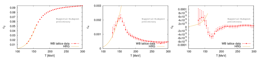
Fig. 1: Taylor coefficients for the equation of state from imaginary $\mu_{B}$ simulations. The data are continuum extrapolated. The errors do not include the systematics of the fitting in $\mu_{B}$.

3 Transition line

We calculated the transition temperature ($T_{c}$) for the four imaginary chemical potentials in the continuum limit. We defined $T_{c}$ with three observables as i) the peak of the renormalized chiral susceptibility normalized to the fourth power of the pion mass, ii) the inflection point of the renormalized chiral condensate, iii) the inflection point of the strangeness susceptibility. The curvature $\kappa$ of the transition line in the QCD phase diagram is defined by the equation

$$\frac{T_{c}(\mu_{B})}{T_{c}(\mu_{B}=0)}=1-\kappa\left(\frac{\mu_{B}}{T_{c}(\mu_{B})}\right)^{2}+\mathcal{O}(\mu_{B}^{4})\,.$$ (1)

Although different definitions are known to give slightly different transition temperatures in the range around 155 MeV [4], they give remarkably consistent curvatures. Our combined result is $\kappa=0.0149\pm 0.0021$ [13]. The transition line can be analytically continued, which we show in Fig. 2. The central transition line corresponds to the inflection point of the chiral condensate, its width shows the error of the extrapolation of the inflection point. The increasing width is only partly coming from the statistical errors. Instead of using Eq. (1) we also allowed a $\mu_{B}^{4}$ term in our fits. At large $\mu_{B}$ this next-to-leading-order contribution drives the extrapolation error and signals the end of the accessible $\mu_{B}$ range.

For recent continuum extrapolated lattice results, though without implementing the strangeness neutrality condition, see Refs. [14, 15].

4 Equation of state

The equation of state at finite density can be accessed through the Taylor coefficients at $\mu_{B}=0$:

$$\frac{p(\mu_{B})}{T^{4}}=c_{0}(T)+c_{2}(T)\left(\frac{\mu_{B}}{T}\right)^{2}+c_{4}(T)\left(\frac{\mu_{B}}{T}\right)^{4}+c_{6}(T)\left(\frac{\mu_{B}}{T}\right)^{6}+\mathcal{O}(\mu_{B}^{8})$$ (2)

The first continuum result for $c_{2}$ was published in Ref. [16]. In the physical point up to $c_{4}$ has recently been calculated, but without continuum extrapolation [17].

The coefficients in Eq. (2) are defined such that strangeness neutrality is implicitly assumed. In other words, $p/T^{4}$ is first expressed as function of $\mu_{S},\mu_{B}$ and $T$, and evaluated at $\mu_{S}(\mu_{B},T)$ for which $\left\langle S\right\rangle=0$. Then Taylor coefficients are defined then for each fixed $T$. Our results also include a $\mu_{Q}$ to meet the actual setting in heavy ion collisions, such that $\left\langle Q\right\rangle=0.4\left\langle B\right\rangle$.

Here we show results for the coefficients from imaginary $\mu_{B}$ simulations. We fitted $c_{2},\dots,c_{6}$ on the $\mu_{B}$-derivatives of $p/T^{4}$ for fixed temperature, $c_{0}$ we determined earlier [7]. The results are shown in Fig. 1.

From the coefficients pressure, energy density, entropy and speed of sound can be calculated at any (small) chemical potential. Here we show one possible application: we calculate the trajectory of the quark gluon plasma on the $T-\mu_{B}$ phase diagram. Since the expansion of the plasma is adiabatic (constant entropy) and the net conserved charges (e.g. baryon number) are constant in a closed system, we can track the trajectory as the constant $s/n$ contours.

For the central bin of each RHIC beam energy down to 19 GeV we find the $s/n$ ratio in the freeze-out points located by the HRG-based analysis of charge and proton fluctuations [18]. Then we draw the entire contour in the phase diagram. We have checked that the trajectory is consistent with the HRG prediction for all collision energies near the freeze-out point. We show the contours and the transition line in Fig. 2.

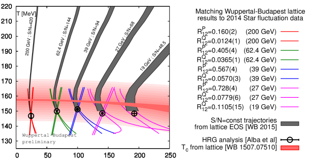
Fig. 2: The QCD phase diagram from analytical continuation. We used lattice simulations with imaginary chemical potentials and extrapolated the transition temperature (red band) to real chemical potentials. We also determined the equation of state. Here we show the constant entropy/net baryon number contours that match chemical freeze-out data. Finally, we show the contours for constant mean/variance ratios of the net electric charge from lattice. We also show the HRG prediction for the proton fluctuation ratios. The contours that correspond to STAR data intersect in the freeze-out points of [18].

5 Freeze-out curve

As an alternative to hadron yields, fluctuations of conserved charges can also be used to find the freeze-out parameters, since lattice has already calculated the equilibrium temperature dependence of many of the fluctuation ratios [19, 20, 10]. The direct comparison of the equilibrium ratios of lattice to experimental reality is not free from ambiguities [21, 22], the study of these goes beyond the scope of this work.

Our results are summarized in Fig. 2. We calculated the net electric charge mean/variance ratios for various imaginary chemical potentials and extrapolated to finite $\mu_{B}$. In Fig. 2 we show the constant $M/\sigma$ contours matching the 2014 STAR data for electric charge fluctuations [23]. To avoid the use of baryon data from lattice as proton fluctuations we simply used the HRG model to calculate the proton fluctuation ratio and matched that to STAR data [24]. If the comparison between lattice and experiment had no additional systematics, the intersection points between these contours would pin-point the freeze-out parameters.

Very recently, a similar study (but using $\mu_{B}=0$ ensembles) have been published, where the $\kappa$ was extracted from fluctuation data [25]. Interestingly the data seem to prefer a negative freeze-out curvature, which is also true in our Fig. 2 and also in [18]. The full systematics of the comparison between lattice and experiment is yet to be understood.

Acknowledgements: This project was supported by the Deutsche Forschungsgemeinschaft grant SFB/TR55. C. Ratti is supported by the National Science Foundation through grant number NSF PHY-1513864. S. D. Katz is funded by the ”Lendület” program of the Hungarian Academy of Sciences ((LP2012-44/2012). An award of computer time was provided by the INCITE program. This research used resources of the Argonne Leadership Computing Facility, which is a DOE Office of Science User Facility supported under Contract DE-AC02-06CH11357. The Gauss Centre for Supercomputing (GCS) has provided computing time as a Large-Scale Project on the supercomputer JUQUEEN.

References

- [1] Y. Aoki, G. Endrodi, Z. Fodor, S. Katz, K. Szabo, Nature 443 (2006) 675–678. arXiv:hep-lat/0611014, doi:10.1038/nature05120.
- [2] Y. Aoki, Z. Fodor, S. Katz, K. Szabo, Phys.Lett. B643 (2006) 46–54. arXiv:hep-lat/0609068, doi:10.1016/j.physletb.2006.10.021.
- [3] Y. Aoki, S. Borsanyi, S. Durr, Z. Fodor, S. D. Katz, et al., JHEP 0906 (2009) 088. arXiv:0903.4155, doi:10.1088/1126-6708/2009/06/088.
- [4] S. Borsanyi, et al., JHEP 1009 (2010) 073. arXiv:1005.3508, doi:10.1007/JHEP09(2010)073.
- [5] A. Bazavov, T. Bhattacharya, M. Cheng, C. DeTar, H. Ding, et al., Phys.Rev. D85 (2012) 054503. arXiv:1111.1710, doi:10.1103/PhysRevD.85.054503.
- [6] S. Borsanyi, G. Endrodi, Z. Fodor, A. Jakovac, S. D. Katz, et al., JHEP 1011 (2010) 077. arXiv:1007.2580, doi:10.1007/JHEP11(2010)077.
- [7] S. Borsanyi, Z. Fodor, C. Hoelbling, S. D. Katz, S. Krieg, et al., Phys.Lett. B730 (2014) 99–104. arXiv:1309.5258, doi:10.1016/j.physletb.2014.01.007.
- [8] A. Bazavov, et al., Phys.Rev. D90 (9) (2014) 094503. arXiv:1407.6387, doi:10.1103/PhysRevD.90.094503.
-
[9]
S. Borsanyi,
in:
Proceedings, 33rd International Symposium on Lattice Field Theory (Lattice
2015), 2015.
arXiv:1511.06541.
URL http://inspirehep.net/record/1405731/files/arXiv:1511.06541.pdf - [10] S. Borsanyi, Z. Fodor, S. Katz, S. Krieg, C. Ratti, et al., Phys.Rev.Lett. 113 (2014) 052301. arXiv:1403.4576, doi:10.1103/PhysRevLett.113.052301.
- [11] M. D’Elia, M.-P. Lombardo, Phys. Rev. D67 (2003) 014505. arXiv:hep-lat/0209146, doi:10.1103/PhysRevD.67.014505.
- [12] P. de Forcrand, O. Philipsen, Nucl.Phys. B642 (2002) 290–306. arXiv:hep-lat/0205016, doi:10.1016/S0550-3213(02)00626-0.
- [13] R. Bellwied, S. Borsanyi, Z. Fodor, J. Günther, S. D. Katz, C. Ratti, K. K. Szabo, Phys. Lett. B751 (2015) 559–564. arXiv:1507.07510, doi:10.1016/j.physletb.2015.11.011.
- [14] C. Bonati, M. D’Elia, M. Mariti, M. Mesiti, F. Negro, F. Sanfilippo, Phys. Rev. D92 (5) (2015) 054503. arXiv:1507.03571, doi:10.1103/PhysRevD.92.054503.
- [15] P. Cea, L. Cosmai, A. PapaarXiv:1508.07599.
- [16] S. Borsanyi, G. Endrodi, Z. Fodor, S. Katz, S. Krieg, et al., JHEP 1208 (2012) 053. arXiv:1204.6710, doi:10.1007/JHEP08(2012)053.
- [17] P. Hegde, Nucl.Phys. A931 (2014) 851–855. arXiv:1408.6305, doi:10.1016/j.nuclphysa.2014.08.089.
- [18] P. Alba, W. Alberico, R. Bellwied, M. Bluhm, V. Mantovani Sarti, et al., Phys.Lett. B738 (2014) 305–310. arXiv:1403.4903, doi:10.1016/j.physletb.2014.09.052.
- [19] A. Bazavov, H. Ding, P. Hegde, O. Kaczmarek, F. Karsch, et al., Phys.Rev.Lett. 109 (2012) 192302. arXiv:1208.1220, doi:10.1103/PhysRevLett.109.192302.
- [20] S. Borsanyi, Z. Fodor, S. Katz, S. Krieg, C. Ratti, et al., Phys.Rev.Lett. 111 (2013) 062005. arXiv:1305.5161, doi:10.1103/PhysRevLett.111.062005.
- [21] A. Bzdak, V. Koch, V. Skokov, Phys.Rev. C87 (2013) 014901. arXiv:1203.4529, doi:10.1103/PhysRevC.87.014901.
- [22] V. Skokov, B. Friman, K. Redlich, Phys.Rev. C88 (2013) 034911. arXiv:1205.4756, doi:10.1103/PhysRevC.88.034911.
- [23] L. Adamczyk, et al., Phys.Rev.Lett. 113 (2014) 092301. arXiv:1402.1558, doi:10.1103/PhysRevLett.113.092301.
- [24] L. Adamczyk, et al., Phys.Rev.Lett. 112 (2014) 032302. arXiv:1309.5681, doi:10.1103/PhysRevLett.112.032302.
- [25] A. Bazavov, et al.arXiv:1509.05786.