Abstract

Local magnetic moments can be created in graphene by incorporating different defects. The possibility of regulating dynamics of magnetization in graphene, by employing the Purcell effect, is analyzed. The role of the system parameters in magnetization reversal is studied. The characteristics of such a reversal can be varied in a wide range, which can be used for various applications in spintronics. It is shown that fast magnetization reversal generates coherent radiation.

Keywords: Magnetic graphene, Magnetization reversal, Spintronics, Coherent radiation

PACS numbers: 75.60.Jk, 75.40.Gb, 75.50.Dd, 76.60.Es

Corresponding author: V.I. Yukalov, E-mail: yukalov@theor.jinr.ru

1 Introduction

Finite quantum systems demonstrate a rich variety of properties that can be employed for numerous applications. Among such finite systems, it is possible to mention quantum dots, nanoclusters, nanomolecules, trapped atoms, etc. [1]. A novel class of finite quantum systems is presented by graphene.

When considering electronic properties of graphene, magnetic effects are usually disregarded, since they occur on much smaller energy scales than other energies [2, 3, 4, 5, 6, 7, 8, 9, 10]. For instance, the Zeeman energy $g\mu_{B}B$, in the external field of $B=1$ T, is only $4.3\times 10^{-5}$ eV ($0.5$ K). This is much smaller than other characteristic energies in the tight-binding form of the electronic Hamiltonian, the nearest-neighbor hopping energy $2.8$ eV ($3.25\times 10^{4}$ K), the next-nearest-neighbor hopping energy $0.1$ eV ($1.16\times 10^{3}$ K, and the electron-electron on-site Coulomb repulsion energy that is of order $1-10$ eV ($10^{4}-10^{5}$ K). Direct spin-spin electron interactions are also small, $\mu_{B}^{2}/a^{3}\approx\rho\mu_{B}^{2}/a\sim 10^{-5}$ eV ($0.2$ K), where $a\approx 1.42$ Å  is carbon-carbon spacing and $\rho\approx 3.9\times 10^{15}$ cm^-2 is the planar density of carbon atoms. The only energy that is smaller than the Zeeman energy is the energy of spin-orbit interactions, which is of order $10^{-6}-10^{-5}$ eV ($0.01-0.1$ K).

Magnetic effects become more pronounced in the presence of disorder that can come about in many different forms, such as adatoms, vacancies, admixtures on the top of graphene or in the substrate, and also extended defects, such as cracks and edges [2, 3, 5, 7, 8, 9, 10, 11]. Adatoms can possess magnetic moments, interacting with electronic spins as in the Kondo problem [12]. Magnetic moments also develop around vacancies. Spins, localized at such defects, interact with each other, either ferromagnetically or antiferromagnetically. Magnetization can be induced at the edges of graphene flakes and quantum dots. A graphene quantum dot of radius $R\sim 100$ nm can have $10-20$ edge spins [7, 13]. A series of quantum dots can form graphene ribbons with disordered edges.

There are numerous works confirming the existence of localized magnetic moments at graphene defects, such as zigzag edges [11, 14, 15, 16, 17, 18], vacancies [19, 20, 21, 22, 23, 24, 25], divacancies [26, 27], adatoms [28, 29, 30], and transition-metal dimers [31]. Hydrogenated zigzag edges [17, 32] can possess local magnetic moments with spins $1/2$, $3/2$, and $5/2$. Such dehydrogenated zigzag-edge groups form dehydrogenated nanomolecules exhibiting ferromagnetism at room temperatures [17, 33]. Examples of these nanomolecules are: C₅₆H₂₂, C₆₄H₂₃, C₅₆H₂₄, C₆₄H₂₅, and C₆₄H₂₇. Zigzag edges can show magnetism in bilayer graphene [34]. Organic substrates on graphene can be magnetized [35]. Strain can also induce magnetism at zigzag edges [36, 37]. In some cases, defects can form magnetic clusters on graphene [38], with spins up to $S=5/2$. Paramagnetic impurities of isolated Mn²⁺ ions also possess spins $S=5/2$ [39].

Various types of defects in graphene are described in the review articles [40, 41]. Emergence of defect-induced magnetism in graphene materials has been reviewed by Yazyev [42] and by Enoki and Ando [43].

Magnetic properties of graphene nanostructures offer unique opportunities for various technological applications related to spintronics, for instance, in quantum information processing. One of the most important requirements for efficient spin manipulation is the possibility to quickly vary the spin direction.

In the present paper, we describe a method allowing for fast magnetization reversal in graphene. We accomplish numerical simulations and analyze the characteristic features of the reversal process. We show that, by employing the Purcell effect [44], that is, coupling the sample to a resonant electric circuit, it is possible to efficiently regulate the magnetization dynamics. Here it is important to remind that under Purcell effect one often understands quantum electrodynamics phenomena exhibiting enhancement of emission processes due to a resonant cavity. However, the meaning of the Purcell effect is more general, implying the enhancement of relaxation phenomena due to coupling with a resonator. Moreover, in his original paper [44] Purcell considered not a cavity electrodynamics phenomena, but the relaxation of a spin system. It is exactly spin dynamics that is the topic of the present paper, and the Purcell effect is understood in its original meaning [44].

We demonstrate that fast magnetization reversal in graphene can generate coherent radiation, whose characteristics depend on the properties of magnetic defects.

2 Model of magnetic graphene

Defects in graphene interact with each other by means of exchange interactions [42, 43] characterized by a Heisenberg Hamiltonian

$$\hat{H}_{def}=-\;\frac{1}{2}\sum_{i\neq j}J_{ij}\left[\left(S_{i}^{x}S_{j}^{x}+S_{i}^{y}S_{j}^{y}\right)+\alpha S_{i}^{z}S_{j}^{z}\right]\;,$$ (1)

where $\alpha$ is an anisotropy parameter and $S_{j}^{\nu}$ is a $\nu$ component of an effective spin of a $j$-th defect, with $j=1,2,\ldots,N$. We take into account the existence of an external magnetic field $B_{0}$ directed along the axis $z$. In order to realize the Purcell effect, the sample is placed inside a magnetic coil of an electric circuit, producing a magnetic field $H$ acting on the defect spins and directed along the coil axis that is taken along the axis $x$. Thus, the total Hamiltonian is

$$\hat{H}=\hat{H}_{def}-\mu_{0}\sum_{j=1}^{N}{\bf B}\cdot{\bf S}_{j}\;,$$ (2)

in which $\mu_{0}$ is a defect magnetic moment and the total magnetic field

$${\bf B}=B_{0}{\bf n}_{z}+H{\bf n}_{x}$$ (3)

is the sum of a constant external field $B_{0}$ along the unit vector ${\bf n}_{z}$ and of a coil magnetic field $H$ along the unit vector ${\bf n}_{x}$. The magnetic moment $\mu_{0}$ is due to electrons and is negative.

The coil magnetic field is a feedback field induced by the moving spins of the sample. The equation for this field follows from the Kirchhoff equation and can be written [45, 46] in the form

$$\frac{dH}{dt}+2\gamma H+\omega^{2}\int_{0}^{t}H(t^{\prime})\;dt^{\prime}=-4\pi\;\frac{dm_{x}}{dt}\;,$$ (4)

in which

$$\gamma\equiv\frac{\omega}{2Q}$$ (5)

is the circuit damping, $\omega$ is the circuit natural frequency, and $Q$ is a resonator quality factor. The effective electromotive force in the right-hand side of the equation is caused by the moving magnetization

$$m_{x}=\frac{\mu_{0}}{V_{res}}\sum_{j=1}^{N}\;\langle S_{j}^{x}\rangle\;,$$ (6)

due to spins of the sample inside the coil of volume $V_{res}$. The angle brackets imply statistical averaging.

The equations of motion for spins are given by the Heisenberg equations

$$i\hbar\;\frac{dS_{j}^{\nu}}{dt}=\left[S_{j}^{\nu},\;\hat{H}\right]\qquad(\nu=x,y,z)\;.$$ (7)

Writing down these equations, we are interested in the temporal behavior of the averaged over the sample spin polarizations

$$e_{\nu}\equiv\frac{1}{NS}\sum_{j=1}^{N}S_{j}^{\nu}\qquad(\nu=x,y,z)\;.$$ (8)

The latter are treated in the mean-field approximation with respect to statistical averaging:

$$\langle e_{\mu}e_{\nu}\rangle=\langle e_{\mu}\rangle\langle e_{\nu}\rangle\;.$$ (9)

For the sake of simplicity, we write in what follows $e_{\nu}$ instead of $<e_{\nu}>$.

The feedback equation (4) defines the feedback magnetic field $H$, for which we introduce the dimensionless quantity

$$h\equiv\frac{H}{B_{0}}\;.$$ (10)

The electric circuit is tuned in resonance with the Zeeman frequency

$$\omega_{0}\equiv\frac{1}{\hbar}\;|\mu_{0}B_{0}|\;,$$ (11)

so that

$$\omega=\omega_{0}\;.$$ (12)

The parameter characterizing the coupling of the sample with the resonator can be defined as

$$\beta\equiv\left|\;\frac{\mu_{0}NS}{B_{0}V_{res}}\;\right|\;.$$ (13)

Differentiating Eq. (4), we come to the feedback equation

$$\frac{d^{2}h}{dt^{2}}+\frac{1}{Q}\;\frac{dh}{dt}+h=4\pi\beta\;\frac{d^{2}e_{x}}{dt^{2}}\;,$$ (14)

where time is measured in units of $1/\omega$. The initial conditions read as

$$h(0)=\dot{h}(0)=0\;,$$ (15)

with the overdot being time derivative.

The total intensity of radiation can be estimated by the formula

$$I=\frac{2}{3c^{3}}\;\left|\ddot{\bf M}\right|^{2}\;,$$

where ${\bf M}$ is the sample magnetization moment

$${\bf M}=\mu_{0}\sum_{j=1}^{N}\langle\bf S_{j}\rangle\;.$$

As we have checked, the sharp peaks in the radiation intensity are due to coherent radiation, but when radiation is spread over a long time interval, it is mainly due to the incoherent part of radiation.

In the following section, we present the results of numerical solution for the equations describing the average spin polarizations $e_{\nu}$ and the corresponding radiation intensity. Our aim is to analyze the influence of the system parameters on the possibility of regulating the dynamics of graphene magnetization, paying the main attention to the influence of these parameters on the time of magnetization reversal, the value of the reversed spin polarization, and the related coherent spin radiation.

3 Defects at zigzag edge

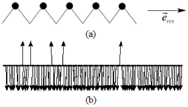
Figure 1: (a) Location of defects at a zigzag edge of a graphene ribbon: (b) initial configuration of defect spins.

We consider the often met situation, when defects with spins are located along a zigzag edge of a graphene ribbon or a graphene flake. This edge is assumed to be directed along the axis $x$ corresponding to the direction of the resonator coil. Such a geometry is taken because it guarantees the best coupling of the resonator with the spins of the sample [47, 48]. The spins of the sample are prepared in a strongly nonequilibrium state, similarly to the setup employed in other magnetic materials [45, 46, 47, 48, 49, 50]. At the initial time, the defect spins are polarized downwards, with the total initial polarization $e_{z}(0)=-0.9$. This initial state is shown in Fig. 1. The sample is placed inside a resonator coil. And an external magnetic field is imposed, for which the equilibrium polarization would correspond to upwards spins. The questions of interest are: how quickly the spins reverse to the upward direction, how this reversal time depends on the system parameters, how the latter influence the value of the reversed magnetization, as well as the strength of the radiation intensity.

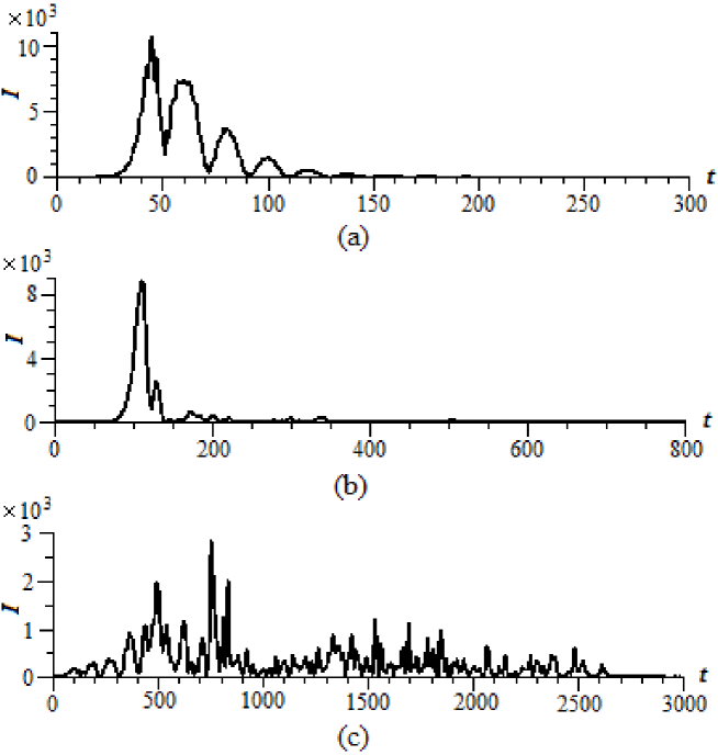
Figure 3: Radiation intensity in units erg/s = $10^{-7}$ W for the same sample parameters as in Fig. 2: (a) $\alpha=1$ (absence of anisotropy); (b) $\alpha=1.2$; and (c) $\alpha=1.4$. Increasing the anisotropy suppresses the radiation intensity.

We accomplish numerical solution of the evolution equations for a chain of $N=100$ defect spins at a zigzag edge. The exchange interactions act only among the nearest neighbors, with the fixed strength $JS=\hbar\omega$, while other parameters are varied. In Fig. 2, we illustrate the role of magnetic anisotropy, characterized by the magnetic anisotropy parameter $\alpha$, for the coupling parameter $\beta=0.01$ and the resonator quality factor $Q=10$. Time is measured in units of $1/\omega$. Increasing the anisotropy makes the reversed value of $e_{z}$ smaller. Thus, when there is no anisotropy $(\alpha=1)$, the polarization reversal is practically complete, with the final polarization $e_{z}\approx 0.9$. Under the anisotropy parameter $\alpha=1.2$, the final $e_{z}\approx 0.75$, and for $\alpha=1.4$, the final $e_{z}\approx 0.7$. The reversal time increases with the increase of the anisotropy. When there is no anisotropy $(\alpha=1)$ the reversal time is $t_{rev}\approx 50$, although there are oscillations before the reversed magnetization stabilizes. For $\alpha=1.2$, the reversal time is $t_{rev}\approx 100$. And for $\alpha=1.4$, this time is $t_{rev}\approx 3000$. The anisotropy suppresses the radiation intensity, as is clear form Fig. 3. In this and in the following figures, the radiation intensity is measured in units of erg/s = $10^{-7}$ W.

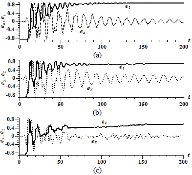
Figure 4: Spin polarizations $e_{x}$ (dotted line) and $e_{z}$ (solid line) versus dimensionless time for the coupling parameter $\beta=0.1$ and the resonator quality factor $Q=10$, for different anisotropy parameters: (a) $\alpha=1$ (no anisotropy); (b) $\alpha=1.2$; and (c) $\alpha=1.4$. Increasing the anisotropy reduces the value of the reversed polarization $e_{z}$, but practically does not change the reversal time.

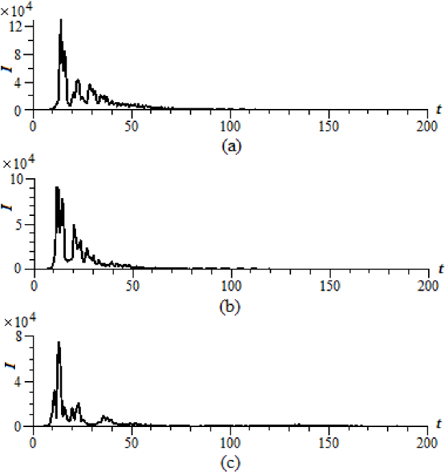
Figure 5: Radiation intensity in units erg/s = $10^{-7}$ W for the same sample parameters as in Fig. 4: (a) $\alpha=1$ (no anisotropy); (b) $\alpha=1.2$; and (c) $\alpha=1.4$. For a larger coupling parameter, the suppression of radiation intensity by the anisotropy is weaker.

The role of anisotropy can be diminished by a stronger coupling with the resonator, as is shown in Fig. 4, where $\beta=0.1$ and $Q=10$. In this figure, the first reversal happens at $t_{rev}\approx 15$ for all anisotropies up to $\alpha=1.5$, although oscillations of $e_{z}$ remain for some time. The final reversed value of $e_{z}$ decreases with increasing anisotropy. The related radiation intensity is shown in Fig. 5.

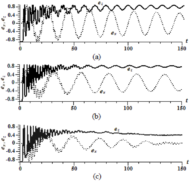
Figure 6: Spin polarizations $e_{x}$ (dotted line) and $e_{z}$ (solid line) versus dimensionless time for the coupling parameter $\beta=1$ and the resonator quality factor $Q=10$, for different anisotropy parameters: (a) $\alpha=1$ (no anisotropy); (b) $\alpha=1.2$; and (c) $\alpha=1.4$. Increasing the anisotropy reduces the value of the reversed polarization $e_{z}$, almost does not change the reversal time, but induces strong oscillations of the spin polarizations.

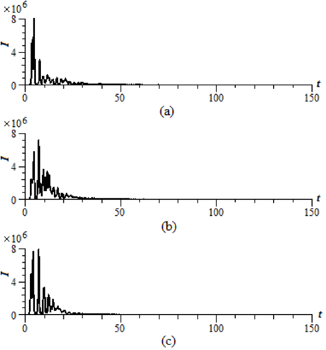
Figure 7: Radiation intensity in units erg/s = $10^{-7}$ W for the same sample parameters as in Fig. 6: (a) $\alpha=1$ (no anisotropy); (b) $\alpha=1.2$; and (c) $\alpha=1.4$. For a larger coupling parameter, the radiation intensity is not strongly suppressed by the anisotropy.

Increasing further the coupling between the sample and the resonator coil, although slightly diminishes the first reversal time, but induces strong oscillations of the spin polarizations, as is illustrated in Fig. 6 for $\beta=1$ and $Q=10$. The stronger coupling with the resonator increases the radiation intensity, as is seen in Fig. 7.

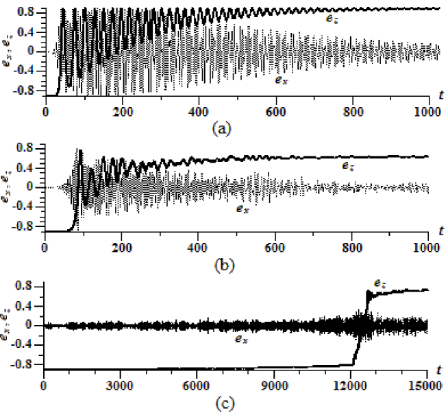
Figure 8: Spin polarizations $e_{x}$ (dotted line) and $e_{z}$ (solid line) versus dimensionless time for the coupling parameter $\beta=0.01$ and the resonator quality factor $Q=100$, for different anisotropy parameters: (a) $\alpha=1$ (no anisotropy); (b) $\alpha=1.2$; and (c) $\alpha=1.4$. Increasing the anisotropy suppresses spin oscillations, only slightly reduces the value of the reversed polarization $e_{z}$, but strongly delays the reversal time.

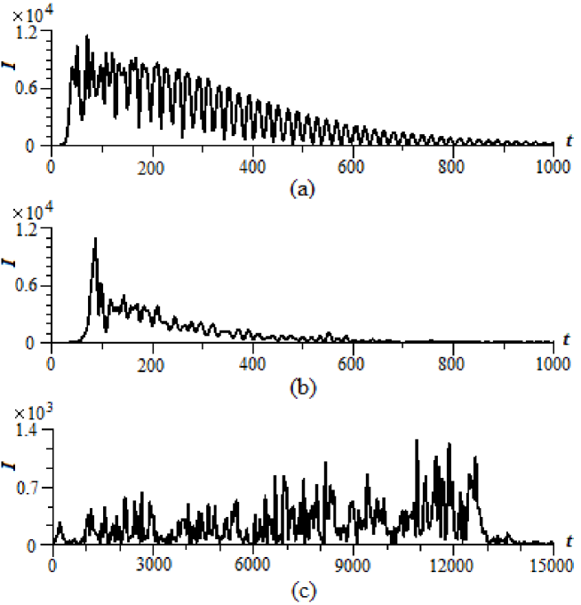
Figure 9: Radiation intensity in units erg/s = $10^{-7}$ W for the same sample parameters as in Fig. 8: (a) $\alpha=1$ (no anisotropy); (b) $\alpha=1.2$; and (c) $\alpha=1.4$. Increasing the resonator quality factor induces many oscillations in radiation intensity.

An intermediate situation occurs when the coupling is weak, but the quality factor is large, say, $\beta=0.01$ and $Q=100$. Then, at small anisotropy, there exist strong oscillations that become suppressed at increasing anisotropy. However, increasing the anisotropy essentially delays the magnetization reversal, as is shown in Fig. 8, and destroys the peak of the radiation intensity, spreading it over a wide time interval, as follows from Fig. 9.

When for applications, it is necessary to achieve a short reversal time, but avoiding strong oscillations, then the optimal regime for this would correspond to not too strong coupling, under weak anisotropy, as in Figs. 2a and 2b. Although increasing the coupling suppresses the role of anisotropy, but leads to strong oscillations that could be undesirable in practical applications, such as information processing.

However, when, on the contrary, it is necessary to increase the reversal time, which could be desirable for information preservation, this can be achieved by increasing the anisotropy.

Since there are numerous ways of producing magnetic graphene by incorporating different defects, as is discussed in the Introduction, the parameters of the system can be varied in a wide range. Therefore this kind of magnetic graphene could provide possibility for different applications in spintronics, e.g., for information processing.

Figure Captions

Figure 1. (a) Location of defects at a zigzag edge of a graphene ribbon: (b) initial configuration of defect spins.

Figure 2. Transverse, $e_{x}$ (dotted line), and longitudinal, $e_{z}$ (solid line), spin polarizations as functions of dimensionless time (measured in units of $1/\omega$), for the coupling parameter $\beta=0.01$ and the resonator quality factor $Q=10$, for different anisotropy parameters: (a) $\alpha=1$, which implies the absence of anisotropy; (b) $\alpha=1.2$; and (c) $\alpha=1.4$. Increasing the anisotropy reduces the value of the reversed polarization $e_{z}$ and increases the reversal time.

Figure 3. Radiation intensity in units erg/s = $10^{-7}$ W for the same sample parameters as in Fig. 2: (a) $\alpha=1$ (absence of anisotropy); (b) $\alpha=1.2$; and (c) $\alpha=1.4$. Increasing the anisotropy suppresses the radiation intensity.

Figure 4. Spin polarizations $e_{x}$ (dotted line) and $e_{z}$ (solid line) versus dimensionless time for the coupling parameter $\beta=0.1$ and the resonator quality factor $Q=10$, for different anisotropy parameters: (a) $\alpha=1$ (no anisotropy); (b) $\alpha=1.2$; and (c) $\alpha=1.4$. Increasing the anisotropy reduces the value of the reversed polarization $e_{z}$, but practically does not change the reversal time.

Figure 5. Radiation intensity in units erg/s = $10^{-7}$ W for the same sample parameters as in Fig. 4: (a) $\alpha=1$ (no anisotropy); (b) $\alpha=1.2$; and (c) $\alpha=1.4$. For a larger coupling parameter, the suppression of radiation intensity by the anisotropy is weaker.

Figure 6. Spin polarizations $e_{x}$ (dotted line) and $e_{z}$ (solid line) versus dimensionless time for the coupling parameter $\beta=1$ and the resonator quality factor $Q=10$, for different anisotropy parameters: (a) $\alpha=1$ (no anisotropy); (b) $\alpha=1.2$; and (c) $\alpha=1.4$. Increasing the anisotropy reduces the value of the reversed polarization $e_{z}$, almost does not change the reversal time, but induces strong oscillations of the spin polarizations.

Figure 7. Radiation intensity in units erg/s = $10^{-7}$ W for the same sample parameters as in Fig. 6: (a) $\alpha=1$ (no anisotropy); (b) $\alpha=1.2$; and (c) $\alpha=1.4$. For a larger coupling parameter, the radiation intensity is not strongly suppressed by the anisotropy.

Figure 8. Spin polarizations $e_{x}$ (dotted line) and $e_{z}$ (solid line) versus dimensionless time for the coupling parameter $\beta=0.01$ and the resonator quality factor $Q=100$, for different anisotropy parameters: (a) $\alpha=1$ (no anisotropy); (b) $\alpha=1.2$; and (c) $\alpha=1.4$. Increasing the anisotropy suppresses spin oscillations, only slightly reduces the value of the reversed polarization $e_{z}$, but strongly delays the reversal time.

Figure 9. Radiation intensity in units erg/s = $10^{-7}$ W for the same sample parameters as in Fig. 8: (a) $\alpha=1$ (no anisotropy); (b) $\alpha=1.2$; and (c) $\alpha=1.4$. Increasing the resonator quality factor induces many oscillations in radiation intensity.

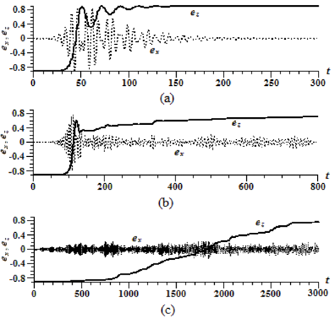
Figure 2: Transverse, $e_{x}$ (dotted line), and longitudinal, $e_{z}$ (solid line), spin polarizations as functions of dimensionless time (measured in units of $1/\omega$), for the coupling parameter $\beta=0.01$ and the resonator quality factor $Q=10$, for different anisotropy parameters: (a) $\alpha=1$, which implies the absence of anisotropy; (b) $\alpha=1.2$; and (c) $\alpha=1.4$. Increasing the anisotropy reduces the value of the reversed polarization $e_{z}$ and increases the reversal time.

References

- [1] Birman J L, Nazmitdinov R G and Yukalov V I 2013 Phys. Rep. 526 1
- [2] Castro Neto A H, Guinea F, Peres N M, Novoselov K S and Geim A K 2009 Rev. Mod. Phys. 81 109
- [3] Abergel D S, Apalkov V, Berashevich J, Ziegler K and Chakraborty T 2010 Adv. Phys. 59 261
- [4] Dresselhaus M S, Jorio A and Saito R 2010 Annu. Rev. Condens. Matter Phys. 1 89
- [5] Goerbig M O 2011 Rev. Mod. Phys. 83 1193
- [6] Saito R, Hofman M, Dresselhaus G, Jorio A and Dresselhaus M S 2011 Adv. Phys. 60 413
- [7] Kotov V N, Uchoa B, Pereira V M, Guinea F and Castro Neto A H 2012 Rev. Mod. Phys. 84 1067
- [8] Katsnelson M I 2012 Graphene: Carbon in Two Dimensions (Cambridge: Cambridge University)
- [9] McCann E and Koshiro M 2013 Rep. Prog. Phys. 76 056503
- [10] Wehling T O, Black-Schaffer A M and Balatsky A V 2014 Adv. Phys. 63 1
- [11] Palacios J J 2010 Semicond. Sci. Technol. 25 033003
- [12] Andrei N, Furuya K and Lowenstein J H 1983 Rev. Mod. Phys. 55 331
- [13] Huang L, Lai Y C, Ferry D K, Akis R and Goodnick S M 2009 J. Phys. Condens. Matter 21 344203
- [14] Enoki T, Kobayashi Y 2005 J. Mater. Chem. 15 3999
- [15] Jiang D E, Sumpter B G and Dai S 2007 J. Chem. Phys. 127 124703
- [16] Otani M, Koshino M, Takagi Y and Okada S 2010 Phys. Rev. B 81 161403
- [17] Gorjizadeh N, Ota N and Kawazoe Y 2013 Chem. Phys. 415 64
- [18] Magda G Z, Jin X, Hagymasi I, Vancso P, Osvath Z, Nemes-Incze P, Hwang C, Biro L P and Tapaszto L 2014 Nature 514 608
- [19] Lisenkov S, Andriotis A N and Menon M 2010 Phys. Rev. B 82 165454
- [20] Chen J H, Li L, Cullen W G, Williams E D and Fuhrer M S 2011 Nature Phys. 7 535
- [21] Nair R R, Sepioni M, Tsai I L, Lehtinen O, Keinonen J, Krasheninnikov A V, Thomson T, Geim A K, and Grigorieva I V 2012 Nature Phys. 8 199
- [22] Yang H X, Chshiev M, Boukhvalov D W, Waintal X and Roche S 2011 Phys. Rev. B 84 214404
- [23] Lopez-Sancho M P, Castro E V and Vozmediano M A 2013 AIP Conf. Proc. 1517 229
- [24] Li Y, He J and Kou S P 2014 Phys. Rev. B 90 201406
- [25] Faccio R and Mombru A W 2015 Comput. Mater. Sci. 97 193
- [26] Bhandary S, Eriksson O and Sanyal B 2013 Sci. Rep. 3 3405
- [27] Jaskolski W, Chio L and Ayuela A 2015 arXiv 1503.08750
- [28] Power S R, de Menezes V M, Fagan S B and Fereira M S 2011 Phys. Rev. B 84 195421
- [29] Pike N A and Stroud D 2014 Phys. Rev. B 89 115428
- [30] Pike N A and Stroud D 2014 Appl. Phys. Lett. 105 052404
- [31] Blonsky P and Hafner J 2014 J. Phys. Condens. Matter 26 256001
- [32] Kabir M and Saha-Dasgupta T 2014 Phys. Rev. B 90 064420
- [33] Qaiumzadeh A and Asgari R 2009 Phys. Rev. B 80 035429
- [34] Zhang Z, Chen C, Zeng X C and Guo W 2010 Phys. Rev. B 81 155428
- [35] Garnica M, Stradi D, Barja S, Calleja F, Dias C, Alcami M, Martin N, Vazquez de Parga A L, Martin F and Miranda R 2013 Nature Phys. 9 368
- [36] Hu T, Zhou J, Dong J M and Kawazoe Y 2013 Phys. Rev. B 87 079906
- [37] Roy B, Assaad F F and Herbut I F 2014 Phys. Rev. X 4 021042
- [38] Boukhvalov D W and Katsnelson M I 2011 ACS Nano 5 2440
- [39] Panich A M, Shames A I and Sergeev N A 2013 Appl. Magn. Res. 44 107
- [40] Terrones H, Lv R, Terrones M and Dresselhaus M S 2012 Rep. Prog. Phys. 75 062501
- [41] Bekyarova E, Sarkar S, Niyogi S, Itkis M E and Haddon R C 2012 J. Phys. D: Appl. Phys. 45 154009
- [42] Yaziev O V 2010 Rep. Prog. Phys. 73 056501
- [43] Enoki T and Ando T 2013 Physics and Chemistry of Graphene (Singapore: Pan Stanford)
- [44] Purcell E M 1946 Phys. Rev. 69 681
- [45] Yukalov V I 1996 Phys. Rev. B 53 9232
- [46] Yukalov V I and Yukalova E P 2004 Phys. Part. Nucl. 35 348
- [47] Yukalov V I, Henner V K, Kharebov P V and Yukalova E P 2008 Laser Phys. Lett. 5 887
- [48] Yukalov V I, Henner V K and Yukalova E P 2015 J. Phys. Conf. Ser. 594 012006
- [49] Davis C L, Kaganov I V and Henner V K 2000 Phys. Rev. B 62 12328
- [50] Henner V, Raikher Y and Kharebov P 2011 Phys. Rev. B 84 144412