Theoretical approaches to the structural properties of the square-shoulder fluid

Abstract

A comparison of simulation results with the prediction of the structural properties of square-shoulder fluids is carried out to assess the performance of three theories: Tang–Lu’s first-order mean spherical approximation, the simplified exponential approximation of the latter and the rational-function approximation. These three theoretical developments share the characteristic of being analytical in Laplace space and of reducing in the proper limit to the Percus–Yevick result for the hard-sphere fluid. Overall, the best agreement with the simulation data is obtained with the simplified exponential approximation.

This paper is dedicated to the memory of Dr. Yiping Tang

1 Introduction

Simple models of the intermolecular potential describing a fluid are often useful to gain insight into many interesting phenomena occurring in real fluids. This is the case of the ‘square-shoulder’ (SS) interaction, a purely repulsive potential, first used in this context by Hemmer and Stell [1, 2], which has been the subject of many papers in the literature, including some rather recent ones [3, 4, 5, 6, 7, 8, 9, 10, 11, 12, 13, 14, 15, 16, 17, 18, 19, 20, 21, 22, 23, 24, 25]. This model may be considered to be the simplest one of the family of core-softened potentials that have been employed to study systems such as water [18], metallic systems [3], colloidal suspensions [5, 6] and aqueous solutions of electrolytes [11]. The expression for the SS potential reads

$$\phi_{\text{SS}}(r)=\left\{\begin{array}[]{ll}\infty,&r<\sigma,\\ \epsilon,&\sigma<r<\lambda\sigma,\\ 0,&r>\lambda\sigma,\end{array}\right.$$ (1)

where $r$ is the distance, $\sigma$ is the diameter of the hard core, $\epsilon>0$ is the shoulder height and $(\lambda-1)\sigma$ is the shoulder width. Note that the thermodynamic properties of the SS fluid only depend on three dimensionless parameters, namely the packing fraction $\eta\equiv(\pi/6)\rho\sigma^{3}$ ($\rho$ being the number density), the reduced temperature $T^{*}=k_{B}T/\epsilon$ ($k_{B}$ and $T$ being the Boltzmann constant and the absolute temperature, respectively) and the width parameter $\lambda$. It is known in particular that the SS potential may lead to an isostructural solid–solid transition [7, 8], to a fluid–solid coexisting line with a maximum melting temperature [4], to unusual phase behaviour [9, 10, 17] and to a rich variety of (self-organised) ordered structures [13, 14, 16, 20].

On the other hand, it is interesting to note that the SS potential becomes equivalent to a hard-sphere (HS) interaction of diameter $\sigma$ in the limits of vanishing shoulder height ($\epsilon\to 0$) or width ($\lambda\to 1$), and to an HS interaction of diameter $\lambda\sigma$ in the limit of infinite shoulder height ($\epsilon\to\infty$). These three limiting situations imply that

$$\lim_{T^{*}\to\infty}g_{\text{SS}}(r;\sigma,\lambda,\eta,T^{*})= g_{\text{HS}}(r;\sigma,\eta),$$ (2a)

$$\lim_{\lambda\to 1}g_{\text{SS}}(r;\sigma,\lambda,\eta,T^{*})= g_{\text{HS}}(r;\sigma,\eta),$$ (2b)

$$\lim_{T^{*}\to 0}g_{\text{SS}}(r;\sigma,\lambda,\eta,T^{*})= g_{\text{HS}}(r;\lambda\sigma,\lambda^{3}\eta),$$ (2c)

where $g_{\text{SS}}(r;\sigma,\lambda,\eta,T^{*})$ is the radial distribution function (RDF) of the SS fluid and $g_{\text{HS}}(r;\sigma,\eta)$ is the RDF of the HS fluid. Also, in the low-density limit one has $g_{\text{SS}}\to e^{-\phi_{\text{SS}}/k_{B}T}$, i.e.

$$\lim_{\eta\to 0}g_{\text{SS}}(r;\sigma,\lambda,\eta,T^{*})=\left\{\begin{array}[]{ll}0,&r<\sigma,\\ e^{-1/T^{*}},&\sigma<r<\lambda\sigma,\\ 1,&r>\lambda\sigma.\end{array}\right.$$ (3)

Furthermore, continuity of $g_{\text{SS}}(r)\exp\left[\phi_{\text{SS}}(r)/T^{*}\right]$ at $r=\lambda\sigma$ implies the exact property

$$g_{\text{SS}}(r=\lambda\sigma^{+};\sigma,\lambda,\eta,T^{*})=g_{\text{SS}}(r=\lambda\sigma^{-};\sigma,\lambda,\eta,T^{*})e^{1/T^{*}}.$$ (4)

Irrespective of all the previous interesting findings, no exact results for the thermodynamic or structural properties of the SS fluid have been derived up to now. Moreover, not even the Percus–Yevick (PY) closure for the Ornstein–Zernike (OZ) integral equation for this system has led to analytical results. Therefore, the available data come from other approximate theories, from numerical solutions of the OZ equation with various closures and from simulation. Lang et al. [12] studied theoretically the SS fluid using the optimised random-phase approximation and the numerical solution of the OZ equation with the Rogers–Young closure, and also performed Monte Carlo (MC) simulations. Zhou and Solana [19] also reported MC simulations for this system and theoretical results based on a bridge function approximation to close the OZ equation. Further simulation data for the SS fluid and a parametrisation of the direct correlation function which quantitatively agrees with the numerical solution of the OZ equation with the PY closure were presented by Guillén-Escamilla et al. [21].

A few years ago, we carried out a theoretical study of the structural properties of this system [23] using the rational-function approximation (RFA) methodology that had been earlier employed successfully for other systems [26, 27]. More recently, Hlushak et al. [24] considered both the Tang–Lu first-order mean spherical approximation(FMSA) [28, 29, 30, 31] and its associated simplified exponential approximation (SEXP/FMSA) [32] for the RDF of the SS fluid and reported additional MC data for the system. These three approaches (FMSA, SEXP/FMSA and RFA) are formulated in terms of the Laplace transform

$$G(s)=\int_{0}^{\infty}dr\,e^{-sr}rg(r)$$ (5)

of $rg(r)$, where, for simplicity, we have dropped the subscript SS and the arguments $(\sigma,\lambda,\eta,T^{*})$. Moreover, the three of them reduce to the exact solution of the PY approximation of the HS fluid (of diameter $\sigma$) [33, 34, 35] in the limits $\lambda\to 1$ or $T^{*}\to\infty$ (see Equations (2a) and (2b)), although only the RFA reduces to such a solution (of diameter $\lambda\sigma$) in the limit $T^{*}\to 0$ (see Equation (2c)). The aim of this paper is to perform a comparison of the results arising in the above three theoretical approximations with simulation data in order to asses the merits and limitations of each formulation.

The paper is organised as follows. In order to make it self-contained, in Section 2 we present the main steps leading to derivation of the structural properties of the SS fluid using the three theoretical approaches referred to above, namely the FMSA, the SEXP/FMSA and the RFA. This is followed in Section 3 by a comparison of the results of the different analytical approximations and those obtained from simulation. The paper is closed in Section 4 with further discussion and some concluding remarks.

2 Radial distribution function of the square-shoulder fluid

2.1 General properties

We begin by recalling general results that apply exactly to fluids whose molecules interact via any intermolecular potential having a hard core at $r=\sigma$, as is the case of the SS fluid. In what follows we will set, without loss of generality, $\sigma=1$. This means that henceforth all distances will be measured in units of the hard-core diameter $\sigma$. In order to determine the structural properties of such fluids, it is convenient to deal with the Laplace transform defined in Equation (5). Also, for later use, we introduce the auxiliary function $F(s)$ defined through [36, 26, 27]

$$G(s)=\frac{sF(s)e^{-s}}{1+12\eta F(s)e^{-s}}.$$ (6)

Due to the hard-core condition $g(r)=0$ for $r<1$, while $g(1^{+})=\text{finite}$, one has

$$g(r)=\Theta(r-1)\left[g(1^{+})+g^{\prime}(1^{+})(r-1)+\cdots\right],$$ (7)

where $g^{\prime}(r)\equiv\partial g(r)/\partial r$ and $\Theta\left(x\right)$ is the Heaviside step function. In view of Equation (7), the large-$s$ behaviours of $G(s)$ and $F(s)$ are constrained, so that

$$e^{s}sG(s)= g(1^{+})+\left[g(1^{+})+g^{\prime}(1^{+})\right]s^{-1}+{\cal O}(s^{-2}),$$ (8a)

$$F(s)= g(1^{+})s^{-2}+\left[g(1^{+})+g^{\prime}(1^{+})\right]s^{-3}+\mathcal{O}(s^{-4}).$$ (8b)

Therefore,

$$\lim_{s\to\infty}e^{s}sG(s)=\lim_{s\to\infty}s^{2}F(s)=g(1^{+})=\text{finite}.$$ (9)

On the other hand, the (reduced) isothermal compressibility is given by

$$\chi\equiv k_{B}T\left(\frac{\partial\rho}{\partial p}\right)_{T}=1+24\eta\int_{0}^{\infty}dr\,r^{2}\left[g(r)-1\right]$$

$$= 1-24\eta\lim_{s\to 0}\frac{\partial}{\partial s}\int_{0}^{\infty}dr\,e^{-sr}r\left[g(r)-1\right]$$

$$= 1-24\eta\lim_{s\to 0}\frac{\partial}{\partial s}\left[G(s)-s^{-2}\right].$$ (10)

Note that $\chi$ must also be finite, and so $\int_{0}^{\infty}dr\,r^{2}\left[g(r)-1\right]=\text{finite}$. Therefore, the weaker condition $\int_{0}^{\infty}dr\,r\left[g(r)-1\right]=\lim_{s\to 0}[G(s)-s^{-2}]=\text{finite}$ must hold. Taking those constraints into account leads to the following small-$s$ behaviours:

$$s^{2}G(s)= 1+\mathcal{O}(s^{2}),$$ (11a)

$$F(s)= -\frac{1}{12\eta}\left[1+s+\frac{s^{2}}{2}+\frac{1+2\eta}{12\eta}s^{3}+\frac{1+\eta/2}{12\eta}s^{4}\right]+\mathcal{O}(s^{5}).$$ (11b)

The introduction of the auxiliary function $F(s)$ in Equation (6) allows us to obtain convenient expressions for the RDF in the coordination shells $n<r<n+1$. We first rewrite Equation (6) as

$$G(s)=\sum_{n=1}^{\infty}\left(-12\eta\right)^{n-1}s\left[F(s)\right]^{n}e^{-ns}.$$ (12)

Then, the RDF may be obtained from

$$g(r)=\frac{1}{r}\sum_{n=1}^{\infty}\left(-12\eta\right)^{n-1}{\psi}_{n}(r-n){\Theta(r-n)},$$ (13)

where $\psi_{n}(r)$ is the inverse Laplace transform of $s\left[F(s)\right]^{n}$.

Clearly, knowledge of $F(s)$ immediately yields $G(s)$ and $g(r)$. Irrespective of how $G(s)$ is determined, once it is available another general result is that the static structure factor $S(q)$ (where $\mathbf{q}$ is the wavevector) of the fluid may be readily obtained from

$$S(q)=1+\rho\int d\mathbf{r}\,e^{-\text{i}\mathbf{q}\cdot\mathbf{r}}[g(r)-1]=1-12\eta\left.\frac{G(s)-G(-s)}{s}\right|_{s=\text{i}q},$$ (14)

where i is the imaginary unit. This confirms the important role played by $G(s)$ in the derivation of the structural properties of hard-core fluids.

2.2 Solution of the Percus–Yevick integral equation for hard-sphere fluids

As is well known, the PY integral equation is exactly solvable for the HS fluid [33, 34, 35]. In such a solution, the Laplace transform is given by Equation (6) with the auxiliary function $F(s)$ expressed as the simplest rational function complying with the physical requirements (9) and (11b) [36, 26, 27]. More specifically,

$$G_{0}(s)=\frac{sF_{0}(s)e^{-s}}{1+12\eta F_{0}(s)e^{-s}},\quad F_{0}(s)=\frac{L_{0}(s)}{R_{0}(s)},$$ (15)

where

$$L_{0}(s)= 1+2\eta+(1+\eta/2)s,$$ (16a)

$$R_{0}(s)= -12\eta(1+2\eta)+18\eta^{2}s+6\eta(1-\eta)s^{2}+(1-\eta)^{2}s^{3}.$$ (16b)

The subscript $0$ in Equation (15) means that the solution is restricted to HS systems with a diameter $\sigma=1$. In the case of HS systems with a diameter $\lambda\sigma=\lambda$, the PY solution is given by Equations (15) and (16) with the replacements $G_{0}\to\lambda^{-2}G_{0}$, $s\to\lambda s$, and $\eta\to\lambda^{3}\eta$ [23]. In real space, according to Equation (13), the HS RDF is given by [37]

$$g_{0}(r)=\frac{1}{r}\sum_{n=1}^{\infty}\left(-12\eta\right)^{n-1}{\psi}_{0n}(r-n){\Theta(r-n)},$$ (17)

with

$$\psi_{0n}(r)= \sum_{j=1}^{n}\frac{\sum_{i=1}^{3}a_{nj}^{(i)}e^{s_{0i}r}}{(n-j)!(j-1)!}r^{n-j}\;,$$ (18a)

$$a_{nj}^{(i)}= \lim_{s\to s_{0i}}\left(\frac{\partial}{\partial s}\right)^{j-1}\left\{s\left[(s-s_{0i})F_{0}(s)\right]^{n}\right\},$$ (18b)

where $\{s_{0i},i=1,2,3\}$ are the three roots of the cubic equation $R_{0}(s)=0$.

2.3 Tang and Lu’s FMSA and SEXP/FMSA for the structural properties of the square-shoulder fluid

In this subsection, we consider the results for the structural properties of the SS fluid as derived from the FMSA and SEXP/FMSA developed by Tang and Lu [29, 30, 32]. The presentation follows very closely the one given for the square-well (SW) fluid in Ref. [38] with the simple replacement of $T^{*}$ by $-T^{*}$.

2.3.1 FMSA

The FMSA theoretical approach, applicable to potentials with a spherical hard core and an arbitrary tail, consists in combining thermodynamic perturbation theory (taking the HS system as the reference fluid) and the mean spherical approximation (MSA) to derive an analytical solution to the OZ equation as a series in powers of the inverse temperature $1/T^{*}$. In the SS fluid case, the expansion of the RDF $g(r)$ to first order reads

$$G(s)= G_{0}(s)+G_{1}(s)\frac{1}{T^{*}},$$ (19a)

$$g(r)= g_{0}(r)+g_{1}(r)\frac{1}{T^{*}},$$ (19b)

where the reference HS functions $G_{0}(s)$ and $g_{0}(r)$ are given by Equations (15) and (17), respectively. The first-order term $G_{1}(s)$ is the opposite of the one for the SW fluid [29, 30], namely

$$G_{1}(s)= \frac{(1-\eta)^{4}}{\left[Q_{0}(s)\right]^{2}}\left\{\frac{s^{4}(1+\lambda s)}{\left[R_{0}(-s)\right]^{2}}e^{-\lambda s}-\sum_{i=1}^{3}\frac{s_{0i}^{3}e^{(\lambda-1)s_{0i}}}{(s+s_{0i})\left[R_{0}^{\prime}(s_{0i})\right]^{2}}e^{-s}\right.$$

$$\left.\times\left[\frac{s_{0i}(1-\lambda s_{0i})}{s+s_{0i}}+s_{0i}(1-\lambda s_{0i})\frac{R_{0}^{\prime\prime}(s_{0i})}{R_{0}^{\prime}(s_{0i})}-4+(1+4\lambda)s_{0i}+\lambda(\lambda-1)s_{0i}^{2}\right]\right\},$$ (20)

where the primes in $R_{0}^{\prime}(s)$ and $R_{0}^{\prime\prime}(s)$ denote derivatives with respect to $s$, and

$$Q_{0}(s)\equiv\frac{R_{0}(s)+12\eta L_{0}(s)e^{-s}}{(1-\eta)^{2}s^{3}}.$$ (21)

As in Equation (18a), the summation over $i$ in Equation (20) extends over the three zeros of $R_{0}(s)$. It is straightforward to find from Equation (20) the jump discontinuity of $g_{1}(r)$ at $r=\lambda$:

$$g_{1}(\lambda^{+})-g_{1}(\lambda^{-})=\lim_{s\to\infty}\frac{s}{\lambda}\frac{(1-\eta)^{4}}{\left[Q_{0}(s)\right]^{2}}\frac{s^{4}(1+\lambda s)}{\left[R_{0}(-s)\right]^{2}}=1.$$ (22)

In what concerns the low-density limit $\eta\to 0$, one has

$$\lim_{\eta\to 0}G_{1}(s)= s^{-2}(1+\lambda s)e^{-\lambda s}-s^{-2}(1+s)e^{-s},$$ (23a)

$$\lim_{\eta\to 0}g_{1}(r)= \Theta(r-\lambda)-\Theta(r-1).$$ (23b)

Performing the inverse Laplace transform of $G_{1}(s)$ one can get explicit expressions for $g_{1}(r)$ inside the shells $n<r<n+1$, which become increasingly more complicated as $n$ grows. Due to the fact that they are not very illuminating and may be found elsewhere [24], they will be omitted here. Alternatively, $G_{1}(s)$ can be numerically inverted [39] to obtain $g_{1}(r)$.

2.3.2 SEXP/FMSA

Now we turn to the SEXP/FMSA [32]. In this theory, the RDF of the SS fluid is approximated by

$$g(r)=g_{0}(r)\exp\left[\frac{g_{1}(r)}{T^{*}}\right],$$ (24)

where $g_{0}(r)$ and $g_{1}(r)$ are those of the FMSA theory. This simplified exponential approximation ensures the positive definite character of the RDF. Notice that the expansion of the SEXP/FMSA (24) to first order in $1/T^{*}$ differs from the FMSA (19b).

In the high-temperature limit $T^{*}\to\infty$, $g(r)\to g_{0}(r)$ both in the FMSA and in the SEXP/FMSA, so that Equation (2a) is verified. A less trivial consistency test corresponds to the limit $\lambda\to 1$. In that case, taking into account the identity

$$\frac{s^{4}(1+s)}{\left[R_{0}(-s)\right]^{2}}=\sum_{i=1}^{3}\frac{s_{0i}^{3}}{(s+s_{0i})\left[R_{0}^{\prime}(s_{0i})\right]^{2}}\left[\frac{s_{0i}(1-s_{0i})}{s+s_{0i}}+s_{0i}(1-s_{0i})\frac{R_{0}^{\prime\prime}(s_{0i})}{R_{0}^{\prime}(s_{0i})}-4+5s_{0i}\right],$$ (25)

one finds that $\lim_{\lambda\to 1}G_{1}(s)=0$, so that $g(r)\to g_{0}(r)$ in that limit, in agreement with Equation (2b). As for conditions (3) and (4), Equations (22) and (23b) show that they are satisfied by the SEXP/FMSA at finite $T^{*}$, but not by the FMSA (except to first order in $1/T^{*}$).

On the other hand, in the zero-temperature limit $T^{*}\to 0$ both the FMSA (19b) and the SEXP/FMSA (24) become singular and none of them complies with Equation (2c).

2.4 The rational-function approximation

We now outline the main steps of the RFA approach to the structural properties of the SS fluid. For further details the reader is referred to Ref. [23].

In the RFA it is assumed that the auxiliary function $F(s)$ in Equation (6) takes the following form

$$F(s)=\frac{L(s)}{R(s)},$$ (26)

where

$$L(s)= 1+2\eta-K^{(0)}+L^{(1)}s+e^{-(\lambda-1)}\left[K^{(0)}+K^{(1)}s\right],$$ (27a)

$$R(s)= -12\eta(1+2\eta)+R^{(1)}s+R^{(2)}s^{2}+R^{(3)}s^{3}.$$ (27b)

Enforcement of Equation (11b) allows one to express the coefficients $L^{(1)}$, $R^{(1)}$, $R^{(2)}$ and $R^{(3)}$ as linear functions of $K^{(0)}$ and $K^{(1)}$:

$$L^{(1)}= 1+\frac{\eta}{2}+(\lambda-1)\frac{2+\eta\left(\lambda^{3}+\lambda^{2}+\lambda+1\right)}{2(1+2\eta)}{K^{(0)}}-\frac{1+2\lambda^{3}\eta}{1+2\eta}{K^{(1)}},$$ (28a)

$$R^{(1)}= {6\eta^{2}}\left[{3}-(\lambda-1)^{2}\frac{\lambda^{2}+2\lambda+3}{1+2\eta}{K^{(0)}}+\frac{4(\lambda^{3}-1)}{1+2\eta}{K^{(1)}}\right],$$ (28b)

$$R^{(2)}= {6\eta}\left[1-\eta-(\lambda-1)^{2}\frac{1-\eta(\lambda+1)^{2}}{1+2\eta}K^{(0)}+2(\lambda-1)\frac{1-2\eta\lambda(\lambda+1)}{1+2\eta}K^{(1)}\right],$$ (28c)

$$R^{(3)}= (1-\eta)^{2}+\eta(\lambda-1)^{2}\frac{4+2\lambda-\eta(3\lambda^{2}+2\lambda+1)}{1+2\eta}K^{(0)}$$

$$-6\eta(\lambda-1)\frac{\lambda+1-2\eta\lambda^{2}}{1+2\eta}K^{(1)},$$ (28d)

Next, application of condition (4) gives [23, 26, 27]

$$\sum_{i=1}^{3}\frac{1+2\eta-K^{(0)}+K^{(1)}s_{i}}{R^{\prime}(s_{i})}s_{i}e^{(\lambda-1)s_{i}}=\frac{K^{(1)}}{\left(e^{1/T^{*}}-1\right)R^{(3)}},$$ (29)

where $\{s_{i},i=1,2,3\}$ are the three roots of the cubic equation $R(s)=0$ and it has been assumed that $\lambda\leq 2$. To close the description, the coefficient $K^{(0)}/(1+2\eta)$ is fixed at its exact zero-density limit value, namely [23]

$$K^{(0)}=(1+2\eta)(1-e^{-1/T^{*}}).$$ (30)

Therefore, Equation (29) becomes a transcendental equation for $K^{(1)}$ that needs to be solved numerically.

Once the coefficients $L^{(1)}$, $R^{(1)}$, $R^{(2)}$, $R^{(3)}$, $K^{(0)}$ and $K^{(1)}$ are determined as functions of $\eta$, $T^{*}$ and $\lambda$ through Equations (28)–(30), $G(s)$ becomes completely specified in the RFA. The RDF $g(r)$ in this case may again be obtained by numerically taking the inverse Laplace transform [39] of the corresponding $G(s)$ or, equivalently, from the use of Equations (26)–(30), together with Equation (13) [27].

It can be easily checked that the RFA is consistent with the exact conditions (2)–(4) [23]. Table 2.4 summarises which ones of those conditions are fulfilled by the FMSA, SEXP/FMSA and RFA approaches.

Summary showing which ones of the exact conditions (2)–(4) are fulfilled by the FMSA, SEXP/FMSA and RFA approaches. Approximation Equation (2a) Equation (2b) Equation (2c) Equation (3) Equation (4) FMSA Yes Yes No No No SEXP/FMSA Yes Yes No Yes Yes RFA Yes Yes Yes Yes Yes

3 Comparison with simulation data

In order to assess the value of the three previous theoretical approximations for the structural properties of SS fluids, in this section we carry out a comparison between the results derived from them and those obtained from simulation [12, 19, 21]. Although we have made such a comparison with many other data, in Figures 1–7 we only show graphs of $g(r)$ vs $r$ for some representative cases.

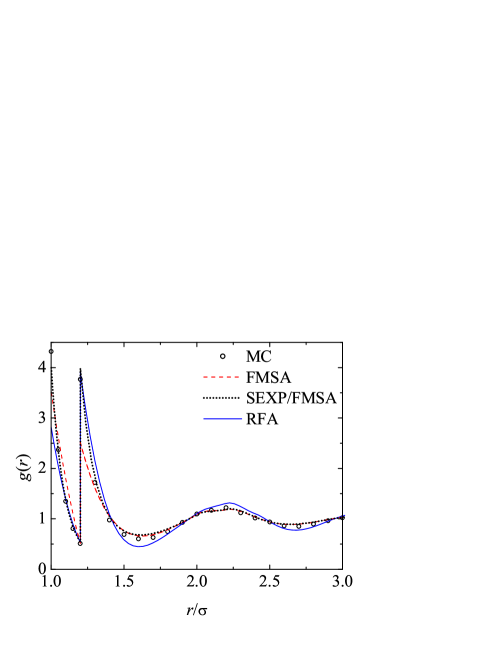
Figure 1: Radial distribution function $g(r)$ as a function of distance $r$ for an SS fluid having $\lambda=1.2$, $T^{*}=0.5$ and $\eta=0.4$ ($\rho\sigma^{3}=0.764$) as obtained from the FMSA (dashed line), the SEXP/FMSA (dotted line), the RFA (solid line) and simulation data from Ref. [12] (circles).

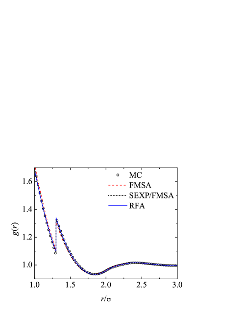
Figure 2: Radial distribution function $g(r)$ as a function of distance $r$ for an SS fluid having $\lambda=1.3$, $T^{*}=5$ and $\eta=0.2094$ ($\rho\sigma^{3}=0.4$) as obtained from the FMSA (dashed line), the SEXP/FMSA (dotted line), the RFA (solid line) and simulation data from Ref. [21] (circles).

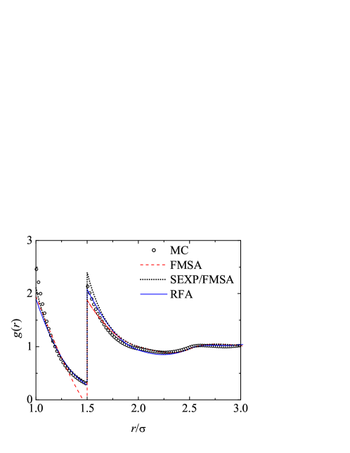
Figure 3: Radial distribution function $g(r)$ as a function of distance $r$ for an SS fluid having $\lambda=1.5$, $T^{*}=0.5$ and $\eta=0.2094$ ($\rho\sigma^{3}=0.4$) as obtained from the FMSA (dashed line), the SEXP/FMSA (dotted line), the RFA (solid line) and simulation data from Ref. [19] (circles).

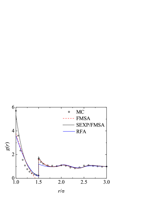
Figure 4: Radial distribution function $g(r)$ as a function of distance $r$ for an SS fluid having $\lambda=1.5$, $T^{*}=0.5$ and $\eta=0.4$ ($\rho\sigma^{3}=0.764$) as obtained from the FMSA (dashed line), the SEXP/FMSA (dotted line), the RFA (solid line) and simulation data from Ref. [12] (circles).

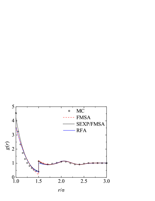
Figure 5: Radial distribution function $g(r)$ as a function of distance $r$ for an SS fluid having $\lambda=1.5$, $T^{*}=1$ and $\eta=0.4$ ($\rho\sigma^{3}=0.764$) as obtained from the FMSA (dashed line), the SEXP/FMSA (dotted line), the RFA (solid line) and simulation data from Ref. [12] (circles).

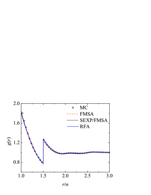
Figure 6: Radial distribution function $g(r)$ as a function of distance $r$ for an SS fluid having $\lambda=1.5$, $T^{*}=2$ and $\eta=0.2094$ ($\rho\sigma^{3}=0.4$) as obtained from the FMSA (dashed line), the SEXP/FMSA (dotted line), the RFA (solid line) and simulation data from Ref. [21] (circles).

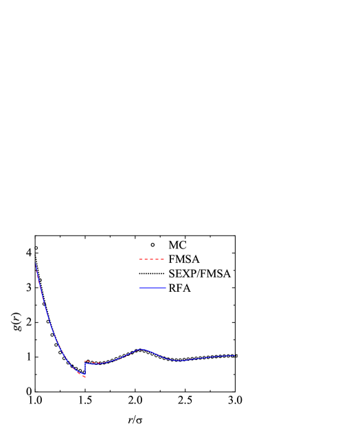
Figure 7: Radial distribution function $g(r)$ as a function of distance $r$ for an SS fluid having $\lambda=1.5$, $T^{*}=2$ and $\eta=0.4189$ ($\rho\sigma^{3}=0.8$) as obtained from the FMSA (dashed line), the SEXP/FMSA (dotted line), the RFA (solid line) and simulation data from Ref. [21] (circles).

Figure 1 displays the RDFs computed with the three theories and the corresponding simulation data for a rather narrow shoulder ($\lambda=1.2$) at relatively low temperature ($T^{*}=0.5$) and high density ($\eta=0.4\Rightarrow\lambda^{3}\eta=0.6912$). It is clear that none of the theories provides a full quantitative agreement with simulation. In particular, the contact value $g(1^{+})$ is underestimated by all of them, with the SEXP/FMSA giving the closest estimate. While $g(\lambda^{-})$ is well accounted for in all instances, in the case of $g(\lambda^{+})$ both the RFA and the SEXP/FMSA do a reasonable job but the FMSA heavily underestimates its value. This is obviously related to the failure of the FMSA to account for the exact relation (4). The location of the maxima and minima of the subsequent oscillations seem to be well captured by all approaches, the RFA exhibiting the poorest agreement with the actual values of the function.

As a representative example of a wider shoulder, Figure 2 presents the case $\lambda=1.3$ at high temperature ($T^{*}=5$) and medium density ($\eta=0.2094$). In this case, the three theories attain very good quantitative agreement, even for the contact value $g(1^{+})$ and the shoulder-edge values $g(\lambda^{-})$ and $g(\lambda^{+})$. At $T^{*}=5$, $e^{1/T^{*}}=1.221\simeq 1+1/T^{*}$ and thus condition (4) can be replaced by its linearised version, which is satisfied by the FMSA. Although not shown, we have checked that the good agreement observed in Figure 2 stays rather reasonable as one increases the packing fraction up to its double value, provided the values of $T^{*}=5$ and $\lambda=1.3$ are maintained.

Next, in Figures 3–7 we fix the standard value $\lambda=1.5$ and analyse the influence of density and, especially, temperature. When $T^{*}=0.5$ and $\eta=0.2094$ (see Figure 3), the situation is somewhat similar to the case in Figure 1, with the contact value being underestimated by all the theories but much less than in the denser system considered in Figure 1. This time, although the quantitative agreement seems not to be bad for both the RFA and the SEXP/FMSA, none of the theories is completely satisfactory. In this instance, it is the RFA the one that does the best job, while the FMSA fails badly, especially in the prediction of both $g(\lambda^{-})$ (that is even negative) and $g(\lambda^{+})$. As the density is increased to $\eta=0.4$ (see Figure 4), the region between contact and $r=\lambda^{-}$ is poorly described by all theories. Further, the RFA underestimates heavily $g(1^{+})$, while both the FMSA and the SEXP/FMSA seem to do a reasonable job for $r>\lambda^{+}$.

Figure 5 corresponds to the same density as in Figure 4, but the temperature has been doubled. Now, as expected, the situation improves for the FMSA. Moreover, the SEXP/FMSA does the best performance.

We keep increasing temperature to $T^{*}=2$ in Figures 6 (corresponding to $\eta=0.2094$) and 7 (corresponding to $\eta=0.4189$). In the former case, the agreement between theories and simulation is very good, with an almost equal performance of the RFA and the SEXP/FMSA, which are both only slightly superior to the FMSA. Comparison between Figures 3 and 6 shows the significant improvement of the FMSA as temperature increases from $T^{*}=0.5$ to $T^{*}=2$. Finally, Figure 7 shows that the trends observed in Figure 6 still hold as one increases the packing fraction, although now the predictions for the contact value somewhat worsen.

It is clear that the poorest performance of all the theoretical developments occurs for relatively low reduced temperatures, as the cases with $T^{*}=0.5$ (see Figures 3 and 4) illustrate. For such temperatures the deficiencies show mostly around the contact region but the theories become less reliable even beyond that region as the packing fraction is increased. The influence of temperature at fixed values of $\lambda$ and $\eta$ may be assessed by comparing Figures 3 and 6. We note that, as the temperature decreases, the contact value increases moderately and also $g(r)$ for $r\gtrsim 2$ becomes more structured. The strongest influence of temperature occurs in the region $r\approx\lambda$ and, as expected on physical grounds, the discontinuity at $r=\lambda$ becomes much more pronounced as the temperature decreases.

Some insight into the effect of the shoulder width on the performance of the theories may be gained by comparing the cases with $T^{*}=0.5$ and $\eta=0.4$ in Figures 1 ($\lambda=1.2$) and 4 ($\lambda=1.5$). One may observe that shrinking the shoulder at fixed temperature and packing fraction makes the theories in general become more reliable, even in a case where the low value of the reduced temperature is less favourable for them. This is not surprising in view of the fact that the SS model becomes closer and closer to the HS model as the shoulder width decreases, as shown by Equation (2b). In this HS limit all three theories reduce to Wertheim–Thiele’s [33, 34, 35] exact solution of the OZ equation with the PY closure. Since the HS potential is also reached from the SS one in the high-temperature limit ($T^{*}\to\infty$) (see Equation (2b)), a better performance of all three approaches can be expected to hold for sufficiently high temperatures. This is confirmed by Figure 2 in the case $\lambda=1.3$, $T^{*}=5$ and $\eta=0.2094$. On the other hand, if the temperature were so low that the situation described by Equation (2c) were approached, the RFA is expected to prevail over the FMSA and SEXP/FMSA.

Before closing this section, it is worth noting that the systems considered in Figures 1, 3 and 4 are the same as those considered in the sixth panel of Figure 2, the third panel of Figure 3 and the sixth panel of Figure 3, respectively, of Ref. [24]. On the other hand, the curves corresponding to the SEXP/FMSA displayed in those figures of Ref. [24] exhibit a higher discrepancy with respect to simulation data than in our Figures 1, 3 and 4. This is due to the fact that, through an involuntary mistake in Ref. [24], the SEXP/FMSA recipe (24) was actually applied only if $g_{1}(r)<0$, while it was replaced by its linearised version $g(r)=g_{0}(r)[1+g_{1}(r)/T^{*}]$ if $g_{1}(r)>0$ [40].

4 Concluding remarks

In this paper we have revisited three analytical procedures [29, 30, 32, 24, 23] to obtain the structural properties of SS fluids and compared their predictions against simulation results [12, 19, 21] in order to assess their merits and limitations. All these approaches have in common the fact that they are analytical in Laplace space and reduce in two independent limits [see Equations (2a) and (2b)] to the PY result for the HS fluid, although only the RFA does it in a third limit [see Equation (2c)]. One should insist on the usefulness of having at hand analytical or semi-analytical approximations for the equilibrium structural properties of simple fluids. In this sense, the FMSA, the SEXP/FMSA and the RFA have once more proved their importance and are simple enough to allow for immediate computations. In a way, the results of the present paper are complementary to those of Refs. [23] and [24], where a (partial) similar analysis was carried out. We have confirmed that the theories lead to reasonably accurate results at any fluid packing fraction if the shoulder is sufficiently narrow (say $\lambda\leq 1.2$), as well as for any width if $\eta$ is small enough ($\eta\leq 0.4$). However, as the width and/or the packing fraction increase, the predictions worsen, especially at low temperatures and in the region between contact and $\lambda$. In any case, from our analysis we can conclude the following. Being a perturbation theory, as expected the FMSA works reasonably well at high temperatures, but worsens as the temperature is reduced, even yielding negative values for $g(\lambda^{-})$, especially when $\lambda$ is increased. The RFA is a reasonable compromise between accuracy and simplicity, but presents some limitations when either the shoulder width or the packing fraction increase. Finally, we found that the best overall performance was shown by the SEXP/FMSA and that it was even better than what was reported in Ref. [24].

Disclosure statement

No potential conflict of interest was reported by the authors.

Funding

The research of Santos Bravo Yuste and Andrés Santos has been partially financed by the Ministerio de Economía y Competitividad (Spain) [grant number FIS2013-42840-P], the Regional Government of Extremadura (Spain) [grant number GR15104] (partially financed by the ERDF).

References

- [1] P.C. Hemmer and G. Stell, Phys. Rev. Lett. 24, 1284 (1970).
- [2] G. Stell and P.C. Hemmer, J. Chem. Phys. 56, 4274 (1972).
- [3] M. Silbert and W.H. Young, Phys. Lett. A 58, 469 (1976).
- [4] D.A. Young and B. Alder, Phys. Rev. Lett. 38, 1213 (1977).
- [5] H. Löwen and G. Kramposthuber, Europhys. Lett. 23, 673 (1993).
- [6] A.A. Louis, E. Allahyarov, H. Löwen and R. Roth, Phys. Rev. E 65, 061407 (2002).
- [7] P. Bolhuis and D. Frenkel, Phys. Rev. Lett. 72, 2211 (1994).
- [8] P. Bolhuis and D. Frenkel, J. Phys.: Condens. Matter 9, 381 (1997).
- [9] C. Rascón, E. Velasco, L. Mederos and G. Navascués, J. Chem. Phys. 106, 6689 (1997).
- [10] L. Mederos, J. Mol. Liq. 76, 139 (1998).
- [11] A. Galindo, A. Gil-Villegas, G. Jackson and N. Burgess, J. Phys. Chem. B 103, 10272 (1999).
- [12] A. Lang, G. Kahl, C.N. Likos, H. Löwen and M. Watzlawek, J. Phys.: Condens. Matter 11, 10143 (1999).
- [13] P. Ziherl and R.D. Kamien, J. Phys. Chem. B 105, 10147 (2001).
- [14] G. Malescio and G. Pellicane, Nat. Mater. 2, 97 (2003).
- [15] V.N. Ryzhov and S.M. Stishov, Phys. Rev. E 67, 010201 (2003).
- [16] G.J. Pauschenwein and G. Kahl, J. Chem. Phys. 129, 174107 (2008).
- [17] S.B. Buldyrev, G. Malescio, C. Angell, N. Giovanbattista, S. Prestipino, F. Saija, H.E. Stanley and L. Xu, J. Phys.: Condens. Matter 21, 504106 (2009).
- [18] N.M. Barraz Jr., E. Salcedo and M.C. Barbosa, J. Chem. Phys. 131, 094504 (2009).
- [19] S. Zhou and J.R. Solana, J. Chem. Phys. 131, 204503 (2009).
- [20] J. Fornleitner and G. Kahl, J. Phys.: Condens. Matter 22, 104118 (2010).
- [21] I. Guillén-Escamilla, E. Schöll-Paschinger and R. Castañeda-Priego, Mol. Phys. 108, 141 (2010).
- [22] M.N. Bannerman and L. Lue, J. Chem. Phys. 133, 124506 (2010).
- [23] S.B. Yuste, A. Santos and M. López de Haro, Mol. Phys. 109, 987 (2011).
- [24] S.P. Hlushak, P.A. Hlushak and A. Trokhymchuk, J. Chem. Phys. 138, 164107 (2013).
- [25] M. Khanpour and R. Hashim, Phys. Chem. Liq. 51, 203 (2013).
- [26] M. López de Haro, S.B. Yuste and A. Santos, Alternative Approaches to the Equilibrium Properties of Hard-Sphere Liquids, in Theory and Simulation of Hard-Sphere Fluids and Related Systems, edited by A. Mulero, Lecture Notes in Physics, Vol. 753 (Springer-Verlag, Berlin, 2008), pp. 183–245.
- [27] A. Santos, A Concise Course on the Theory of Classical Liquids. Basics and Selected Topics, Lecture Notes in Physics, in press (Springer-Verlag, Berlin, 2016).
- [28] Y. Tang and B.C.-Y. Lu, J. Chem. Phys. 99, 9828 (1993).
- [29] Y. Tang and B.C.-Y. Lu, J. Chem. Phys. 100, 3079 (1994).
- [30] Y. Tang and B.C.-Y. Lu, J. Chem. Phys. 100, 6665 (1994).
- [31] Y. Tang, J. Chem. Phys. 118, 4140 (2003).
- [32] Y. Tang and B.C.-Y. Lu, AIChE J. 43, 2215 (1997).
- [33] M.S. Wertheim, Phys. Rev. Lett. 10, 321 (1963).
- [34] M.S. Wertheim, J. Math. Phys. 5, 643 (1964).
- [35] E. Thiele, J. Chem. Phys. 39, 474 (1963).
- [36] S.B. Yuste and A. Santos, Phys. Rev. A 43, 5418 (1991).
- [37] A. Santos 2013, “Radial Distribution Function for Hard Spheres”, Wolfram Demonstrations Project, http://demonstrations.wolfram.com/RadialDistributionFunctionForHardSpheres/.
- [38] J. Largo, J.R. Solana, S.B. Yuste and A. Santos, J. Chem. Phys. 122, 084510 (2005).
- [39] J. Abate and W. Whitt, Queueing Syst. 10, 5 (1992).
- [40] S.P. Hlushak, private communication.