Critical scaling in the large-$N$ $O(N)$ model in higher dimensions and its possible connection to quantum gravity

Abstract

The critical scaling of the large-$N$ $O(N)$ model in higher dimensions using the exact renormalization group equations has been studied, motivated by the recently found non-trivial fixed point in $4<d<6$ dimensions with metastable critical potential. Particular attention is paid to the case of $d=5$ where the scaling exponent $\nu$ has the value $1/3$, which coincides with the scaling exponent of quantum gravity in one fewer dimensions. Convincing results show that this relation could be generalized to arbitrary number of dimensions above five. Some aspects of AdS/CFT correspondence are also discussed.

In loving memory of my grandmother.

I Introduction

The non-trivial critical behavior in $O(N)$ theories are well-known for dimensions $d<4$ on . Thus, a statement on the existence of interacting critical theories beyond four space-time dimensions is rather unusual since one would expect the triviality of the $O(N)$ vector model in general triv . However, in recent works kleb1 ; kleb2 ; Gracey , exhaustive one, three and four loop analyses of the $O(N)$ theory with cubic interactions and $N+1$ scalars show that the large-$N$ $O(N)$ theory could follow the asymptotically safe scenario under the renormalization group in the UV. More precisely, it was argued that the IR fixed point found in the aforementioned $O(N)$ theory with the cubic interaction is equivalent to a perturbatively unitary UV fixed point in the large-$N$ $O(N)$ model for dimensions $4<d<6$. The presence of such UV fixed point could be particularly interesting due to the conjectured AdS_d+1/CFT_d duality between a higher-spin $d+1$-dimensional massless gauge theory in AdS space (with an appropriate boundary condition) and the large-$N$ critical $O(N)$ model in $d$ dimensions hs . The former is called the Vasiliev theory, which describes a minimal interacting theory with gravity and higher-spin fields in its spectrum. It can be obtained as the tensionless limit of string theory, where the infinite tower of higher-spin string modes are massless, and since there is no energy scale it can be considered as a toy model describing physics beyond the Planck scale vas . Studies related to the existence of the UV fixed point in the large-$N$ $O(N)$ model, using conformal bootstrap approach and exact (or functional) renormalization group (ERG or FRG) methods, can be found in Rey ; boot1 ; boot2 and perc1 ; mati1 , respectively.
The structure of the paper is the following. In section II a discussion of the previous results on the UV fixed point are given. It is shown that the solution by polynomial expansion coincides with one of the infinite many solutions (the physically most sensible one) of the exact treatment. In section III the non-trivial critical scaling for higher dimensional theories is derived. In IV a speculation on the possible connection to quantum gravity is presented.

II Identifying the UV fixed point

First, a brief review of the analytical results from perc1 is given. Let us consider the effective average action of the O($N$) symmetric theory in $d$ dimensions within the local potential approximation (LPA):

$$\Gamma_{k}=\int d^{d}x\left[\frac{1}{2}(\partial\bar{\phi})^{2}+U_{k}(\bar{\phi}^{2})\right].$$ (1)

$U_{k}$ is the dimensionful potential depending on $\bar{\phi}^{2}$, where $\bar{\phi}$ is the dimensionful vacuum expectation value (VEV) of the field. The subscript $k$ stands for the RG scale i.e., the Wilsonian cutoff, which defines the effective theory. In the large-$N$ limit the anomalous dimension of the Goldstone modes disappears, therefore, setting the wave function renormalization constant to unity in (1) gives a well-justified approximation. In fact, the LPA is considered to be exact in the large-$N$ limit of the $O(N)$ model zinn ; zinn2 ; analy . The flow of the effective action is given by the exact functional differential equation FRGgen

$$\partial_{t}\Gamma_{k}=\frac{1}{2}\text{Tr}\left(\Gamma_{k}^{(2)}+R_{k}\right)^{-1}\partial_{t}R_{k}.$$ (2)

Here, the logarithmic flow parameter $t=\ln({k}/{\Lambda})$ (where $\Lambda$ is the initial UV scale) is introduced with a momentum dependent regulating function $R_{k}(q^{2})$ which ensures that the fluctuations above the Wilsonian cutoff scale are integrated out. $\Gamma_{k}^{(2)}[\bar{\phi}]$ is used as a shorthand notation for the second derivative with respect to the field and the trace denotes the integration over all momenta as well as the summation over internal indices. This integral is evaluated by choosing $R_{k}(q^{2})$ so that $\Gamma_{k}$ approaches the bare action in the limit $k\rightarrow\Lambda$ and the full quantum effective action when $k\rightarrow 0$ FRGgen . A detailed study of an extensive class of regulator functions is reported in CSS . In the current case, the optimized regulator is chosen $R_{k}(q^{2})=(k^{2}-q^{2})\,\theta(k^{2}-q^{2})$ which provides an analytic result for the momentum integral opt_rg . It is convenient to introduce $\bar{\rho}\equiv\frac{1}{2}\bar{\phi}^{2}$, which will be used throughout this paper. Inserting (1) into (2) and applying the limit $N\to\infty$ yields the flow for the effective potential in the large-$N$ analy :

$$\partial_{t}u=-du+(d-2)\rho u^{\prime}+\frac{1}{1+u^{\prime}},$$ (3)

where the dimensionless quantities $u=Uk^{-d}$ with $\rho=\bar{\rho}k^{-d+2}$ are introduced and $u^{\prime}=\partial_{\rho}u$.

An exact solution for the $\rho$ derivative of (3) can be obtained by using the method of characteristics analy ; Marchais and the fixed point solutions associated to (3) can be given as an implicit function $\rho=\rho(u_{*}^{\prime})$. $u_{*}$ is introduced as the dimensionless effective potential at the fixed point. The most compact form of these exact solutions for $d=2n+1$ and $d=2n$ ($n\in{\mathbb{Z}}$) are respectively

$$\rho=cu_{*}^{\prime\frac{d}{2}-1}+\frac{1}{(d-2)}\,_{2}F_{1}\left(2,1-\frac{d}{2};2-\frac{d}{2};-u_{*}^{\prime}\right)$$ (4)

and

$$\rho=\bar{c}u_{*}^{\prime\frac{d}{2}-1}+\frac{1}{(d+2)(1+u_{*}^{\prime})^{2}}\,_{2}F_{1}\left(1,2;2+\frac{d}{2};\frac{1}{1+u_{*}^{\prime}}\right),$$ (5)

where $c$ is an arbitrary constant obtained from the integration, $\bar{c}=c-\frac{d\pi}{4}\sin(d\pi/2)$ and ${}_{2}F_{1}$ is the hypergeometric function. Fig. 1 shows the solutions for the case in $d=5$. Each curve corresponds to a solution with a particular value of the parameter $c$. $u_{*}^{\prime}\geq 0$ (4) holds for every $c\in\mathbb{R}$ but in order to obtain a continuation of the solutions to $u_{*}^{\prime}\leq 0$ the constant $c$ needs to take imaginary values.

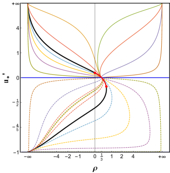
Figure 1: Each curve corresponds to a critical potential derivative with a particular choice of $c$ in $d=5$. The thick black line is for the $c=0$ solution. The red line segment is considered as the physical branch. The axes are rescaled for clarity.

There is one exception: the solution corresponding to $c=0$. This is shown in Fig. 1 as the thick black curve that passes smoothly through $u_{*}=0$ and intersects the horizontal and vertical axes at $\rho=1/3$ and $u_{*}^{\prime}(0)\approx 0.1392$ on the upper plane, respectively. It is tempting to consider this fixed point potential as the physical one since it is analytic at its extremum. On the other hand, this curve still has the problem like the other solutions (including their continuation): $u_{*}^{\prime}$ can be only considered as a multivalued function of $\rho\in[0,0.6214]$ perc1 .

Focus now shifts to the author’s previous results mati1 where a different technique, based upon polynomial expansion, was used to find the fixed point solutions of the flow equation. The potential is assumed to be analytic in this case:

$$u(\rho)=\lim\limits_{n\to\infty}\sum\limits_{i=1}^{n}\frac{u^{(i)}(0)}{i!}\rho^{i}.$$ (6)

The derivatives of the potential are the couplings of the theory: $u^{\prime}(0)=g_{1}=m^{2}$ (squared mass), $u^{\prime\prime}(0)=g_{2}=\lambda$ (quartic coupling), etc… An efficient algorithm was worked out for finding the fixed points of the theory for expansions up to order 50, if required. This method is based on the observation that all the couplings can be expressed through the squared mass of the system at the fixed points, $g_{i}^{*}=g_{i}^{*}(m_{*}^{2})$.

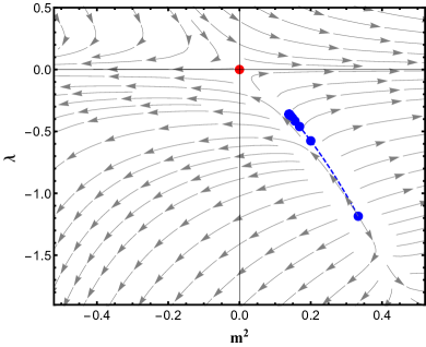
Figure 2: The RG flow in the $\{m^{2},\lambda\}$ hyperplane of theory space. The drifting of the non-trivial UV fixed point is shown towards $\{m_{*}^{2},\lambda_{*}\}\approx\{0.1392,-0.3613\}$ with increasing expansion order (blue dots). The red dot at the origin represents the GFP. Arrows point from UV to IR scales.

In the case of the five-dimensional large-$N$ $O(N)$ model, the fixed point structure shows a non-trivial fixed point as well as the non-interacting Gaussian fixed point (GFP). The fixed point position drifts as the order of the Taylor-expansion increases and converges to $m_{*}^{2}\approx 0.1392$ as shown in Fig. 2. As $m^{2}=u^{\prime}(0)$, it can be confidently stated that this is the same fixed point solution as found by the analytic study of the flow when $c=0$ in (4). In fact, this technique naturally singles out a fixed point solution from all the other solutions that are present only in the analytical case. In Fig. 1 this corresponds to the red line segment on the thick black curve and will be considered as the physical solution.

Fig. 3 shows the comparison between the exact critical potential, computed from (4), and the polynomial expansion results, $u_{*}(\rho)=\sum_{i=1}^{n}\frac{g^{*}_{i}(m_{*}^{2})}{i!}\rho^{i}$, with $n=26$. The non-analytic nature of the exact potential is very apparent as it is restricted to the finite interval unlike to the polynomial potential which was assumed to be analytical. The most important features of this potential are the metastable ground state and the lack of a true vacuum. This may initially discourage further investigations, but metastable and unstable vacua are not unknown. There is the question on the electroweak vacuum stability for instance: it is still a topical question if the Higgs potential exhibits a ground state or if there is an unstable universe existing in a false vacuum (with a very long lifetime) Higgsgen . Alternatively, the theory with the metastable potential could be saved from the AdS side, too. As mentioned above, the critical large-$N$ $O(N)$ theory in $d=5$ is possibly dual to a Vasiliev higher-spin theory in AdS₆ space, thus they must have the same energy spectrum. In AdS space, the Breitenlohner-Freedman (BF) bound gives a negative, dimension dependent lower bound for the squared mass of the field, above which the theory can be considered as stable BFree .

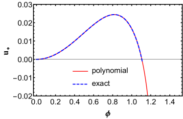
Figure 3: The metastable critical potential in $d=5$. On the horizontal axis the field VEV ($\phi=\sqrt{2\rho}$) was used hence the exact potential is only valid between $\phi\in[0,1.1148]$.

The BF bound can also be generalized for massless higher-spin fields that also depends on the spin value BFreemless . In turn, the same argument could hold for the other branch of $u_{*}^{\prime}(\rho)<0$ for $\rho\in[0,0.6214]$ with $u_{*}^{\prime}(0)=m_{*}^{2}\approx-0.5776$, Fig. 1. In this case the potential is completely unstable in the restricted interval as $u^{\prime}(\rho)<0$. However, this fixed point potential is completely ignored by the polynomial approach.

III Critical scaling

Despite the unconventional properties of the potential, it is still possible to extract the critical exponent $\nu$. This is the scaling exponent of the correlation length (or inverse mass) and characterizes the system at criticality. For the exact determination of the exponent in $d$ dimensions the method of eigenperturbation is used, which is based on the linearized flow around the fixed point, i.e. $u(\rho,t)=u_{*}(\rho)+\delta u(\rho,t)$ Marchais ; eigp . Using (3) the fluctuation equation for the derivative of the potential reads:

$$\partial_{t}\delta u^{\prime}=2\frac{u_{*}^{\prime}}{u_{*}^{\prime\prime}}\left(\partial_{\rho}-\frac{(u_{*}^{\prime}u_{*}^{\prime\prime})^{\prime}}{u_{*}^{\prime}u_{*}^{\prime\prime}}-\frac{d-4}{2}\frac{u_{*}^{\prime\prime}}{u_{*}^{\prime}}\right)\delta u^{\prime}.$$ (7)

This can be thought of as an eigenvalue problem: $\partial_{t}\delta u^{\prime}=\theta\delta u^{\prime}$, where the smallest eigenvalue $\theta$ equals the negative inverse of the scaling exponent $\nu$. Solving this PDE via the method of separation of variables yields

$$\delta u^{\prime}\propto e^{t\theta}u_{*}^{\prime\frac{1}{2}(\theta+d-2)}u_{*}^{\prime\prime}.$$ (8)

The details of this computation are provided in the Appendix. Perturbations at the node ($u_{*}^{\prime}(\rho_{0})=0$) are required to have a high regularity so restrictions on the values of $\theta$ are necessary in order to keep $\delta u^{\prime}$ analytic. Both formulae in (4) and (5) at $u_{*}^{\prime}=0$ take the value $\rho(0)\equiv\rho_{0}=1/(d-2)$. Using Taylor expansion around $\rho_{0}$, and setting $c=0$ and $\bar{c}=0$, a linear behavior of $u_{*}^{\prime}$ can be found, $u_{*}^{\prime}\propto\left(\rho-\frac{1}{d-2}\right)$. This makes $u_{*}^{\prime\prime}$ a constant and substituting back this expression into (8) gives

$$\delta u^{\prime}\propto e^{t\theta}\left(\rho-\frac{1}{d-2}\right)^{\frac{1}{2}(\theta+d-2)}.$$ (9)

The allowed values are then $\theta=2(l+1-d/2)$, where $l$ is a non-negative integer, and the scaling exponent is obtained by the lowest value of $\theta$, i.e. for $l=0$. Thus, the scaling exponent for arbitrary dimensions in the large-$N$ $O(N)$ model is

$$\nu=(d-2)^{-1}.$$ (10)

By using the polynomial expansion, the critical exponent $\nu$ can be calculated as the negative inverse of the lowest eigenvalue of the stability matrix at the fixed point $B_{ij}=\left.\partial\beta_{i}/\partial g_{j}\right|_{g=g_{*}}$ FRGgen , where the beta functions are defined as the RG scale derivative of the couplings: $\beta_{i}=\partial g_{i}(t)/\partial t$. As the LPA became exact in the large-$N$ limit, the correct value for the critical exponent can be obtained at every order of the expansion, i.e. (10) for arbitrary dimensions. This relation, on the other hand, is well-known for the large-$N$ $O(N)$ theories in $d\leq 4$ zinn ; zinn2 ; kardar ; Cardy . However, it was not extended to higher dimensions as the upper critical dimension was considered to be $d=4$. Yet, with an accurate analysis of the fixed point structure for $d>4$, it seems that a non-trivial fixed point can be found in the UV, where, instead of the mean-field scaling, the relation (10) still holds. However, the effective potentials defined at criticality are non-analytic and/or metastable for these values of $d$ and care must be taken with interpreting these results. In particular, in five dimensions $\nu=1/3$ and the ground state seems to be metastable. In the papers kleb1 ; kleb2 also an unbounded critical potential is expected, and in that respect, the results presented here are consistent with those.

Although in the large-$N$ limit the dimensionality is restricted to $4<d<6$ due to the unitarity bound kleb1 ; kleb2 ; unitarity1 , higher dimensional cases can be also studied. Fig. 4 displays the solutions (4) and (5) for $d>5$ with $c=0$ and $\bar{c}=0$, respectively. The following observations can be made. In $d=6,8$ dimensions $u_{*}^{\prime}$ is singular at $\rho=0$ and multivalued for $\rho<\rho_{0}$, in addition, the function (5) also gets complex for $u_{*}^{\prime}\in[0,-1]$ making the theory non-unitary. In $d=7$ the potential seems to be stable but, because of the turning points, it becomes multivalued, although at $\rho=0$ it is unique. In $d=9$ the situation is very similar to Fig. 1 for the $c=0$ case. These three categories seem to be preserved to all even, $d=4n+3$ and $d=4n+1$ ($n\geq 1$) dimensions, respectively. In the even-dimensional case, it is very hard to give a physical interpretation due to its singular structure and complex nature. For the $d=4n+3$ cases, three branches can be defined due to the ”S” shape of the curve around $u^{\prime}_{*}=0$, making it challenging to understand its physical content. Perhaps certain parts of the ”S” shape could be removed in the spirit of Maxwell’s construction max , which would allow us to define a bounded but non-analytic function. When $d=4n+1$, the same arguments as in $d=5$ case can be used to define a metastable potential.

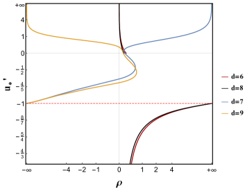
Figure 4: The fixed point solutions given by (4) and (5) in $d\geq 6$ for $c=0$ and $\bar{c}=0$, respectively. The axes are rescaled for clarity.

It is also worth mentioning that a similar convergence to Fig. 2 can be observed clearly only for $4<d<6$ ($d\in\mathbb{R}$) by using the polynomial approximation. From the analytical side, using (4), these solutions have the same structure as in Fig. 1. This might suggest that physically sensible fixed points exist in $4<d<6$, provided that metastability is accepted. However, although the relation for the scaling exponent $\nu$ holds naively for all $d$, further investigations are required for the $d\geq 6$ cases both for integer and fractal dimensions. A recent study related to higher dimensional $O(N)$ theories can be found in Gracey2 .

IV On the possible connection to quantum gravity

Attention now switches to an interesting observation which might link the large-$N$ $O(N)$ model to quantum Einstein gravity (QEG). Much of the current evidence suggests that QEG admits a continuous phase transition between physically two distinct phases described by a strong and weak Newton’s coupling QEG1 . This phenomenon is naturally associated to a UV fixed point which is characterized by a non-trivial scaling of the correlation length: $\xi\propto\left|G_{b}-G_{*}\right|^{-\nu}$, where the dimensionless quantities $G_{b}$ and $G_{*}$ are the bare and the fixed point Newton’s coupling, respectively. Within the framework of FRG in Falls , using the optimized regulator and a special reparametrization of the metric fluctuation that ensures the gauge independence, $\nu^{-1}=-6+4/d+2d$ can be obtained. Substitution of $d=4$ results $\nu=1/3$. The scaling exponent $\nu\simeq 1/3$ has been found by using the Regge lattice action in Hamber’s extensive numerical studies Hamber3 ; Hamber4 ; Hamber5 . A simple geometrical argument is given in support of the exact value of $1/3$ Hamber4 . It is based on the observation that the quantum correction to the static gravitational potential, due to the vacuum-polarization induced scale dependence of Newton’s coupling, can be interpreted as a uniform mass distribution surrounding the original source only if $\nu^{-1}=d-1$ for $d\geq 4$. In particular, for $d=4$ this gives $\nu=1/3$. This conjecture can be compared to the results obtained in Falls by inserting different values for $d$ greater than four: $\nu(d=5)\approx 0.2083$, $\nu(d=6)=0.15$. Moreover, these $\nu$ values might improve by taking into account higher order curvature invariants in the effective action. These results suggest that an interesting relationship can be revealed between the critical exponents of the large-$N$ $O(N)$ model ($\nu_{O}$) and QEG ($\nu_{G}$) as a function of dimension:

$$\nu_{O}(d)\simeq\nu_{G}(d-1),\qquad\text{for }d\geq 5.$$ (11)

A similar phenomenon in critical systems, called Parisi-Sourlas dimensional reduction, shows that particular classical field theories and a corresponding quantum field theory in two fewer dimensions could fall into the same universality class dimred ; dimred5 ; dimred6 ; branched1 ; branched2 . It is highly non-trivial whether the underlying mechanism is the same in the present case, however, two dimensional difference can be found between the classical Vasiliev theory and quantum gravity. Another observation could further support the interesting relation which is conjectured by (11): both QEG and the large-$N$ $O(N)$ model can be related to branched polymer systems. Being more precise, it is widely believed that QEG is described by a branched polymer-like system in its weakly coupled phase Hamber3 ; Hamber4 ; Hamber5 ; GravPolymer . Similarly, $O(N)$ models represent discretized branched polymers at the double scaling limit (i.e. when $N\to\infty$ and $g\to g_{*}^{i}$ in a correlated manner) zinn2 ; OnPolymer . In particular, for $d=5$ equation (11) can be considered to be exact (provided that the QEG exponent is exactly $1/3$), and as it is pointed out in Hamber3 , the critical exponent $\nu=1/3$ possibly corresponds to a branched polymer system: in $d=4$ the exponent $\nu_{p}=1/2$ and at the upper critical dimension $d=8$, $\nu_{p}=1/4$ (where the lower index $p$ stands for ’polymer’). One would expect a branched polymer system with $\nu_{p}=1/3$ for $d\in(4,8)$. Another interesting remark can be made by considering the results of Gracey2 where also some interdimensional universality is shown between different field theories. Considering all these results, it might be possible that a more fundamental connection is emerging in the $d$-dimensional view of these various theories. Despite the relation found in (11) the two theory does not necessarily fall into the same universality class, unless there is way to relate all the critical exponents. There is already a conflict between the most conventional value of the anomalous dimension of the graviton in QEG ($\eta_{G}=-2$) and $\eta_{O}=0$. However, if the usual scaling laws kardar are assumed to be valid in QEG, $\eta_{G}=-2$ in $d=4$ gives $\delta_{G}\to\infty$, which is rather questionable for a critical exponent. It would be of interest to find out if the relationship described in (11) is a mere coincidence or if there is a deeper explanation that implies a correspondence between QEG_d-1 and the large-$N$ $O(N)$ theory in $d$ dimensions which is in turn dual to the higher-spin Vasiliev theory in AdS_d+1 space (where $d\geq 5$).

Appendix A Appendix

In the following the derivation of the eigenperturbation is presented in details. Differentiating (3) with respect to $\rho$ yields:

$$\partial_{t}u^{\prime}=-2u^{\prime}+(d-2)\rho u^{\prime\prime}-\frac{u^{\prime\prime}}{(1+u^{\prime})^{2}}.$$ (12)

The $u^{\prime}(\rho,t)$ solution of this equation is assumed to be accurately described by a small perturbation around the fixed point solution $u^{\prime}(\rho,t)=u_{*}^{\prime}(\rho)+\delta u^{\prime}(\rho,t)$, hence

$$\partial_{t}\delta u^{\prime}= -2(u_{*}^{\prime}+\delta u^{\prime})+(d-2)\rho(u_{*}^{\prime}+\delta u^{\prime})^{\prime}$$ (13)

$$-(u_{*}^{\prime}+\delta u^{\prime})^{\prime}F(u_{*}^{\prime}+\delta u^{\prime}),$$

where $F(u^{\prime})=1/(1+u^{\prime})^{2}$ is introduced, and $\partial_{t}u_{*}^{\prime}$ vanishes by definition. Expanding it around the fixed point solution up to linear order gives

$$F(u_{*}^{\prime}+\delta u^{\prime})\approx F(u_{*}^{\prime})+\frac{\partial F}{\partial u^{\prime}}(u^{\prime}_{*})\delta u^{\prime}.$$ (14)

Thus, considering the last term in (13)

$$(u_{*}^{\prime}+\delta u^{\prime})^{\prime}F\approx (u_{*}^{\prime}+\delta u^{\prime})^{\prime}\left[F(u_{*}^{\prime})+\frac{\partial F}{\partial u^{\prime}}(u^{\prime}_{*})\delta u^{\prime}\right]$$ (15)

$$= u_{*}^{\prime\prime}F(u_{*}^{\prime})+\delta u^{\prime\prime}F(u_{*}^{\prime})+u_{*}^{\prime\prime}\frac{\partial F}{\partial u^{\prime}}(u^{\prime}_{*})\delta u^{\prime},$$

where the last term coming from the product in the right-hand side is neglected since the perturbation assumed to be small. The solution of the fixed point equation satisfies

$$-2u_{*}^{\prime}+(d-2)\rho u_{*}^{\prime\prime}-u_{*}^{\prime\prime}F(u_{*}^{\prime})=0,$$ (16)

hence

$$\partial_{t}\delta u^{\prime}=-2\delta u^{\prime}+(d-2)\rho\delta u^{\prime\prime}-\delta u^{\prime\prime}F\left(u_{*}^{\prime}\right)-u_{*}^{\prime\prime}\frac{\partial F}{\partial u^{\prime}}\left(u^{\prime}_{*}\right)\delta u^{\prime},$$

which can be recast into the following form

$$\partial_{t}\delta u^{\prime}= -2\delta u^{\prime}+(d-2)\rho\delta u^{\prime\prime}-\delta u^{\prime\prime}\left(\rho(d-2)-2\frac{u_{*}^{\prime}}{u_{*}^{\prime\prime}}\right)$$ (18)

$$-\delta u^{\prime}\left((d-2)-2\frac{\partial}{\partial\rho}\frac{u_{*}^{\prime}}{u_{*}^{\prime\prime}}\right),$$

where the relation $\partial F/\partial u^{\prime}=1/u^{\prime\prime}\partial F/\partial\rho$ is used and $F(u_{*}^{\prime})$ is expressed from (16). Further manipulating the right-hand side gives

$$\partial_{t}\delta u^{\prime}=-d\delta u^{\prime}+2\frac{u_{*}^{\prime\prime 2}-u_{*}^{\prime}u_{*}^{\prime\prime\prime}}{u_{*}^{\prime\prime 2}}\delta u^{\prime}+2\frac{u_{*}^{\prime}}{u_{*}^{\prime\prime}}\delta u^{\prime\prime},$$ (19)

which after some algebra provides the final result for the fluctuation equation

$$\partial_{t}\delta u^{\prime}=2\frac{u_{*}^{\prime}}{u_{*}^{\prime\prime}}\left(\partial_{\rho}-\frac{(u_{*}^{\prime}u_{*}^{\prime\prime})^{\prime}}{u_{*}^{\prime}u_{*}^{\prime\prime}}-\frac{d-4}{2}\frac{u_{*}^{\prime\prime}}{u_{*}^{\prime}}\right)\delta u^{\prime}.$$ (20)

The solution of the PDE in (20) is found by using the method of separation of variables, that is $\delta u^{\prime}=f(t)g(\rho)$. A straightforward computation gives

$$f(t)\propto\exp{\theta t}\qquad\text{and}\qquad g(\rho)\propto u_{*}^{\prime\frac{1}{2}(\theta+d-2)}u_{*}^{\prime\prime}.$$ (21)

Thus, the complete solution up to a constant factor

$$\delta u^{\prime}(t,\rho)\propto e^{\theta t}u_{*}^{\prime\frac{1}{2}(\theta+d-2)}u_{*}^{\prime\prime},$$ (22)

where $\theta\in\mathbb{R}$ is given by the regularity condition described in the text.

References

- (1) R. Guida, J. Zinn-Justin, J. Phys. A 31, 8103 (1998); J. Zinn-Justin, Phys. Rept. 344, 159 (2001);B. Delamotte, D. Mouhanna, M. Tissier, Phys. Rev. B 69 134413 (2004); J. M. Caillol, Condensed Matter Physics 16, 43005 (2013); N. Dupuis, Phys. Rev. E 83 031120 (2011); V. Branchina, E. Messina, D. Zappala, Int. J. Mod. Phys. A 28 (2013) 1350078; D. Zappala, Phys.Rev. D 86 (2012) 125003; D. F. Litim, Dario Zappala, Phys. Rev. D 83, 085009 (2011); N. Defenu, P. Mati, I. G. Márián, I. Nándori, A. Trombettoni, JHEP 1505 (2015) 141.
- (2) M. Aizenman, Phys.Rev.Lett. 47, 1-4 (1981); J. Frohlich, Nucl.Phys. B 200, 281-296 (1982); M. Luscher, P. Weisz, Nucl.Phys. B 290, 25 (1987); M. Luscher, P. Weisz, Nucl.Phys. B 295, 65 (1988); M. Luscher, P. Weisz, Nucl.Phys. B 318, 705 (1989); I. Montvay, G. Munster, U. Wolff, Nucl.Phys. B 305, 143 (1988); Ulli Wolf, Phys. Rev. D 79, 105002 (2009).
- (3) L. Fei, S. Giombi, I. R. Klebanov Phys. Rev. D 90, 025018 (2014).
- (4) L. Fei, S. Giombi, I. R. Klebanov, G. Tarnopolsky Phys. Rev. D 91, 045011 (2015).
- (5) J. A. Gracey, Phys. Rev. D 92, 025012 (2015).
- (6) I. R. Klebanov, A. M. Polyakov, Phys. Lett. B 550, 213-219 (2002); X. Bekaert, E. Joung, and J. Mourad, Fortsch. Phys. 60, 882-888 (2012); J. Maldacena, A. Zhiboedov, Class. Quant. Grav. 30, 104003 (2013); S. Giombi, I. R. Klebanov JHEP 1312, 068 (2013); S. Giombi, I. R. Klebanov, B. R. Safdi, Phys.Rev. D 89, 084004 (2014).
- (7) E. S. Fradkin, M. A. Vasiliev, Ann. Phys. 177, 63 (1987); E. S. Fradkin, M. A. Vasiliev, Nucl. Phys. B 291, 141 (1987); E. S. Fradkin and M. A. Vasiliev, Phys. Lett. B 189, 89-95 (1987); M.A. Vasiliev, Phys. Lett. B 243, 378-382 (1990); X. Bekaert, N. Boulanger and P. Sundell, Rev.Mod.Phys. 84, 987-1009 (2012); V.E. Didenko, E.D. Skvortsov, ”Elements of Vasiliev theory”, arXiv:1401.2975 [hep-th].
- (8) J. B. Bae, S. J. Rey, arXiv:1412.6549 [hep-th].
- (9) S. M. Chester, S. S. Pufu, R. Yacoby Phys.Rev. D 91, 086014 (2015).
- (10) Y. Nakayama, T. Ohtsuki. Phys.Lett. B 734, 193-197 (2014).
- (11) R. Percacci, G. P. Vacca, Phys.Rev. D 90, 107702 (2014).
- (12) P. Mati, Phys.Rev. D 91, 125038 (2015).
- (13) J. Zinn-Justin, Quantum Field Theory and Critical Phenomena, Oxford University Press, third edition 1996.
- (14) M. Moshe, J. Zinn-Justin, Phys.Rept. 385, 69-228 (2003).
- (15) N. Tetradis, D.F. Litim, Nucl.Phys. B 464, 492-511 (1996).
- (16) A. Ringwald and C. Wetterich, Nucl. Phys. B 334, 506 (1990); U. Ellwanger, Z. Phys. C 62, 503 (1994); C. Wetterich, Nucl. Phys. B 352, 529 (1991); C. Wetterich, Phys. Lett. B 301, 90 (1993); N. Tetradis, C. Wetterich, Nucl. Phys. B 422 [FS], 541 (1994); T.R. Morris, Int. J. Mod. Phys. A 9, 2411 (1994); T.R. Morris, Phys. Lett. B 329, 241 (1994).
- (17) I. Nándori, JHEP 1304, 150 (2013).
- (18) D. F. Litim, Phys. Lett. B 486, 92 (2000); D. F. Litim, Phys. Rev. D 64, 105007 (2001); D. F. Litim, JHEP 0111, 059 (2001).
- (19) E. Marchais, ”Infrared Properties of Scalar Field Theories”, Ph.D. Thesis , 2012, University of Sussex.
- (20) H. D. Politzer and S. Wolfram, Phys. Lett. B 82, 242 (1979); B 83, 421(E) (1979); P. Q. Hung, Phys. Rev. Lett. 42, 873 (1979); S. Coleman, F. D. Luccia, Phys. Rev. D 21, 3305 (1980); M. S. Turner, F. Wilczek, Nature 298, 633-634 (1982); O. Lebedev, A. Westphal Phys.Lett. B 719, 415-418 (2013); A. Hook, J. Kearney, B. Shakya, K. M. Zurek, JHEP 1501, 061 (2015).
- (21) P. Breitenlohner, D.Z. Freedman; Phys. Lett. B 115, 197 (1982). P. Breitenlohner, D. Z. Freedman, Ann. Phys. 144, 249-281 (1982); D. Marolf, S. F. Ross, JHEP 11, 085 (2006);
- (22) H. Lu, Kai-Nan Shao, Phys. Lett. B 706, 106-109 (2011).
- (23) D.F. Litim, Nucl.Phys. B 631, 128-158 (2002). D. F. Litim, M. C. Mastaler, F. Synatschke-Czerwonka, A. Wipf, Phys.Rev. D 84, 125009 (2011); O.J. Rosten, Physics Reports 511, 177-272 (2012).
- (24) M. Kardar, Statistical Physics of Fields, Cambridge University Press, Cambridge, 2007.
- (25) J. Cardy Scaling and renormalization in statistical physics, Cambridge University Press, Cambridge, 1996.
- (26) G. Parisi, Nucl.Phys. B 100, 368 (1975); G. Parisi, On non-renormalizable interactions, in New Developments in Quantum Field Theory and Statistical Mechanics Cargese 1976, pp. 281–305. Springer US, 1977; X. Bekaert, E. Meunier, and S. Moroz, Phys.Rev. D 85, 106001 (2012).
- (27) J. C. Maxwell, Nature 11: 357–359 (1875); Reichl, L. E. (2009). A Modern Course in Statistical Physics (3rd ed.). New York, NY USA: Wiley-VCH.
- (28) J. A. Gracey, arXiv:1512.04443 [hep-th].
- (29) W. Souma, Prog. Theor. Phys. 102, 181 (1999); O. Lauscher and M. Reuter, Phys. Rev. D 65, 025013 (2002); O. Lauscher and M. Reuter, Phys. Rev. D 66, 025026 (2002); D. F. Litim, Phys.Rev.Lett. 92, 201301 (2004); P. Fischer, D. F. Litim, Phys.Lett. B 638, 497 (2006); A. Codello, R. Percacci, Phys. Rev. Lett. 97, 221301 (2006); A. Codello, R. Percacci, C. Rahmede, Int. J. Mod. Phys. A 23, 143 (2008); A. Codello, R. Percacci, C. Rahmede, Annals Phys. 324, 414 (2009); P. F. Machado, F. Saueressig, Phys. Rev. D 77, 124045 (2008); D. Benedetti, F. Caravelli, JHEP 1206, 017 (2012); J. A. Dietz, T. R. Morris, JHEP 1301, 108 (2013); S. Nagy, B. Fazekas, L. Juhász, K. Sailer, Phys. Rev. D 88, 116010 (2013); S. Nagy, Annals Phys. 350, 310-346 (2014); N. Christiansen, B. Knorr, J. M. Pawlowski, A. Rodigast, (2014), arXiv:1403.1232 [hep-th]; K. Falls.Phys. Rev. D 92, 124057 (2015).
- (30) K. Falls, arXiv: 1503.06233 [hep-th].
- (31) H. W. Hamber, Phys.Rev. D 61, 124008 (2000);
- (32) H. W. Hamber, Ruth M. Williams, Phys. Rev. D 70, 124007 (2004);
- (33) H. W. Hamber, Phys. Rev. D 92, 064017 (2015).
- (34) Y. Imry, S.K. Ma, Phys. Rev. Lett. 35, 1399-1401 (1976); G. Grinstein, Phys Rev. Lett. 37, 944-947 (1976); A. Aharony, Y. Imry, S.K. Ma, Phys. Rev. Lett. 37, 1364-1367 (1976); A.P. Young, J. Phys. C 10, L257-L262 (1977).
- (35) G. Parisi, N. Sourlas, Phys. Rev. Lett. 43, 744-745 (1979).
- (36) A. Klein, L. J. Landau, J. F. Perez, Commun. Math. Phys. 94, 459-482 (1984).
- (37) G. Parisi, N. Sourlas Phys. Rev. Lett. 46, 871 (1981).
- (38) D. C. Brydges, J. Z. Imbrie, Ann. of Math. 158, 1019-1039 (2003); D. C. Brydges, J.Z. Imbrie, J. Statist. Phys. 110, 503–518 (2003).
- (39) M. Reuter and F. Saueressig, Phys. Rev. D 65, 065016 (2002); P. Horava, Phys. Rev. Lett. 102, 161301 (2009); A. Ashtekar and J. Lewandowski, Class. Quant. Grav. 21, R53 (2004).
- (40) J. Zinn-Justin, Phys.Lett. B257 (1991) 335-340; P. Di Vecchia, M. Kato, N. Ohta, Int.J.Mod.Phys. A7 (1992) 1391-1414; M. Moshe in Les Houches 1997, New non-perturbative methods and quantization on the light cone 147-153.