Analytical results for non-linear Compton scattering in short intense laser pulses

Abstract

We study in detail the strong-field QED process of non-linear Compton scattering in short intense plane wave laser pulses of circular polarization. Our main focus is placed on how the spectrum of the back-scattered laser light depends on the shape and duration of the initial short intense pulse. Although this pulse shape dependence is very complicated and highly non-linear, and has never been addressed explicitly, our analysis reveals that all the dependence on the laser pulse shape is contained in a class of three-parameter master integrals. Here we present completely analytical expressions for the non-linear Compton spectrum in terms of these master integrals. Moreover, we analyse the universal behaviour of the shape of the spectrum for very high harmonic lines.

1 Introduction

The non-linear Compton scattering of high-intensity laser pulses off high-energetic electrons is one of the fundamental processes in strong-field QED. Its theoretical description goes back to the 1960’s where many strong-field QED processes had been studied in a series of seminal papers (Nikishov & Ritus, 1964b, a, 1965; Goldman, 1964; Brown & Kibble, 1964). For instance, these authors predicted the emission of high harmonics and a non-linear intensity-dependent red-shift of the emitted radiation, which is proportional to $a_{0}^{2}$, where $a_{0}$ is the dimensionless normalized laser amplitude that is related to the laser intensity ($I$) and wavelength ($\lambda$) via $a_{0}^{2}=0.73\times I[$10^{18}\text{\,}\mathrm{W}\mathrm{/}\mathrm{c}\mathrm{m}^{2}$]\lambda^{2}[\mathrm{\SIUnitSymbolMicro}\mathrm{m}]$. In a classical picture the generation of high harmonics and the non-linear red-shift of the emitted radiation can be understood as the influence of the laser’s magnetic field due to the $\boldsymbol{v}\times\boldsymbol{B}$ term in the classical Lorentz force equation.

However, while most contemporary high-intensity laser facilities generate laser pulses with femtosecond duration (Mourou et al., 2006; Korzhimanov et al., 2011; Di Piazza et al., 2012), most of the early papers on non-linear Compton scattering did not consider the effect of the finite duration of the intense laser pulse. For a realistic laser pulse with a finite duration the laser intensity gradually increases from zero to its maximum value. Consequently, the non-linear red-shift is not constant during the course of the laser pulse and the harmonic lines of the emitted radiation are considerably broadened, with a large number of spectral lines for each harmonic (Narozhnyi & Fofanov, 1996; Boca & Florescu, 2009; Seipt & Kämpfer, 2011; Hartemann & Kerman, 1996; Hartemann et al., 1996, 2010; Mackenroth & Di Piazza, 2011; Dinu, 2013). In the classical picture this broadening is caused by a gradual slow-down of the longitudinal electron motion as the laser intensity ramps up (Seipt et al., 2015a). The occurrence of the additional line structure can be interpreted as interference of the radiation that is emitted during different times (Seipt & Kämpfer, 2013b). The broadening of the spectral lines is especially important with regard to the application of non-linear Compton scattering as an x- and gamma-ray radiation source (Jochmann et al., 2013; Sarri et al., 2014; Rykovanov et al., 2014; Seipt et al., 2015a; Khrennikov et al., 2015).

For ultra-high laser intensities $a_{0}\gg 1$ the formation time of the emitted photon is much shorter than the laser period and the interference of radiation that is emitted at different times during the course of the pulse is suppressed (Dinu et al., 2015). In this regime, where the Compton emission becomes vital for the formation of QED cascades, the spectrum can be effectively simulated using the photon emission probabilities in a constant crossed field (Ritus, 1985; Fedotov et al., 2010; King et al., 2013; Harvey et al., 2015; Narozhny & Fedotov, 2015). We therefore focus in this paper on the intermediate intensity region $a_{0}\sim 1$, where the interference matters and a general relation between the shape and duration of the laser pulse and the shape of the spectrum of the backscattered light is very complicated and highly non-linear. The shape of the harmonic lines is determined by an interplay between the laser pulse duration, (ii) spectral composition of the pulse and (iii) the non-linear ponderomotive broadening which depends on the laser intensity ramps.

In this paper we analytically analyse the non-linear Compton scattering process in a short intense plane wave laser pulse of circular polarization. Our analysis is based on the framework of strong-field QED, where the electrons are described as Volkov states, and we employ the slowly varying envelope approximation. For convenience, the analysis is performed in incident electron frame of reference. In particular, we investigate how the duration and the shape of the short intense laser pulse affect the spectrum of the emitted radiation. We derive a scale invariant master integral that contains all dependence on the shape of the laser pulse, and we give explicit analytical expressions for several specific laser pulse shapes. Our paper is organized as follows: In Section 2 we briefly outline the calculation of the transition amplitude and the energy and angular differential emission probability for non-linear Compton scattering using Volkov states in a pulsed laser field. The transition amplitude is analysed further in Section 3 where we extract the dependence on the duration and shape of the laser pulse in the form of a master integral. Explicit analytic expressions for the master integrals for different pulse shapes are given in Section 3.4. Throughout the paper we use units with $\hbar=c=1$. Scalar products between four-vectors are denoted by $a\cdot b\equiv a^{\mu}b_{\mu}=a^{0}b^{0}-\boldsymbol{a}\boldsymbol{b}$, and the Feynman slash notation is used for scalar products between four-vectors and the Dirac matrices: $\not{a}\equiv\gamma\cdot a$.

2 Theoretical Background

The non-linear Compton scattering process, i.e. the emission of a photon by an electron under the action of an intense laser field, is conveniently described theoretically in the Furry picture. The interaction of the electrons with the laser pulse is treated non-perturbatively by using Volkov electron states $\Psi$ as solutions of the Dirac equation $(i\not{\partial}-e\not{A}-m)\Psi=0$ in the plane-wave background laser field $A$. Here $m$ and $e=-|e|$ denote the mass and charge of the electron, respectively. By employing these Volkov states and the strong-field $S$ matrix in the Furry picture can be represented by the Feynman diagram in Fig. 1. It is given by the expression

$$S=-ie\int\!\mathrm{d}^{4}x\,\mathrm{bar}\Psi_{p^{\prime}}(x)\gamma_{\mu}{\mathcal{A}}^{\mu}_{k^{\prime}}(x)\Psi_{p}(x)\,,$$ (1)

where $\mathcal{A}^{\mu}_{k^{\prime}}(x)=(\varepsilon^{\prime*})^{\mu}e^{ik^{\prime}\cdot x}$ is the amplitude for the emission of a (non-laser) photon with four momentum $k^{\prime}$ and polarization $\varepsilon^{\prime}$, while $p$ and $p^{\prime}$ are the asymptotic four-momenta of the electron before and after the photon emission.

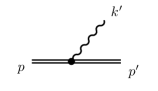
Figure 1: Feynman diagram for the emission of a photon with four-momentum $k^{\prime}$ (wiggly line) by a laser-dressed Volkov electron with asymptotic four-momentum $p$ (double-line). After the photon emission the electron has the asymptotic four-momentum $p^{\prime}$. The double-lines indicate the non-perturbative interaction of the electron with the intense short laser pulse.

In the following, we shall restrict our discussion to the case of a circularly polarized laser pulse with the four-vector potential in the axial gauge ($k\cdot A=0$)

$$A^{\mu}(\phi)=A_{0}\,g(\phi)\>{\Real}\>\epsilon_{+}^{\mu}e^{-i\phi}\,$$

It depends only on the phase variable $\phi=k\cdot x$ with the laser photon four-momentum $k=(\omega,0,0,-\omega)$, and with the normalized polarization four-vector $\epsilon_{\pm}^{\mu}=(0,1,\pm i,0)/\sqrt{2}$, with $\epsilon_{+}\cdot\epsilon_{-}=-1$. The dimensionless normalized laser amplitude is given by $a_{0}=|e|A_{0}/m$. The shape of the laser pulse is described by an envelope function $g(\phi)$, that depends on $\phi$ only via the ratio $\phi/\Delta\phi$ with the pulse duration $\Delta\phi$. Moreover, we use symmetric pulse envelopes with $g(\phi)=g(-\phi)$, $g(0)=1$ and $g(\pm\infty)=0$. For the following we shall assume that the laser pulse consists of several optical cycles such that $\Delta\phi\gg 1$ and we may employ the slowly varying envelope approximation.

One can perform the spatial integrations in the $S$ matrix most conveniently in light-front coordinates, defined as $x^{\pm}=x^{0}\pm x^{3}$ and $\boldsymbol{x}^{\perp}=(x^{1},x^{2})$, such that the laser phase is proportional to $\phi=\omega x^{+}$, and $\mathrm{d}^{4}x=(2\omega)^{-1}\mathrm{d}\phi\mathrm{d}x^{-}\mathrm{d}^{2}\boldsymbol{x}^{\perp}$. After integrating over three light-front coordinates, the $S$ matrix can be represented in a form (Seipt & Kämpfer, 2013a)

$$S=-ie(2\pi)^{3}\delta_{\mathrm{l.f.}}(p-p^{\prime}-k^{\prime})\,\mathrsfs M(s)$$ (2)

with the light-front delta function $\delta_{\mathrm{l.f.}}(p-p^{\prime}-k^{\prime})=\frac{1}{\omega}\delta^{2}(\boldsymbol{p}_{\perp}-\boldsymbol{p}_{\perp}^{\prime}-\boldsymbol{k}_{\perp}^{\prime})\delta(p^{+}-p^{\prime+}-k^{\prime+})$, enforcing the conservation of three momentum components, and the transition amplitude

$$\mathrsfs M=\mathrsfs T_{0}\mathrsfs C_{0}+\mathrsfs T_{+}\mathrsfs C_{+}+\mathrsfs T_{-}\mathrsfs C_{-}+\mathrsfs T_{2}\mathrsfs C_{2}\,.$$ (3)

Here, the quantities $\mathrsfs T_{j}$ denote the transition operators

$$\mathrsfs T_{0} =\mathrm{bar}u_{p^{\prime}}\not{\varepsilon}^{\prime*}u_{p}\,,$$

$$\mathrsfs T_{\pm} =\frac{ma_{0}}{4}\,\mathrm{bar}u_{p^{\prime}}\left(\frac{\not{\varepsilon}_{\pm}\not{k}\not{\varepsilon}^{\prime*}}{(k\cdot p^{\prime})}+\frac{\not{\varepsilon}^{\prime*}\not{k}\not{\varepsilon}_{\pm}}{(k\cdot p)}\right)u_{p}\,,$$ (4)

$$\mathrsfs T_{2} =\frac{m^{2}a_{0}^{2}\,(\varepsilon^{\prime*}\cdot k)}{4(k\cdot p)(k\cdot p^{\prime})}\,\mathrm{bar}u_{p^{\prime}}\not{k}u_{p}\,,$$

which are sensitive to the spin of the incident and final electrons (via the spinors $u_{p}$ and $\mathrm{bar}u_{p^{\prime}}$) and the polarization of the emitted photon. However, they are only weakly dependent on the energy and momentum of the emitted photon. The dependence on the dynamics of the scattering process is mainly contained in the so-called dynamic integrals over the laser phase

$$\mathrsfs C_{\pm 1} =\intop_{-\infty}^{\infty}\!\mathrm{d}\phi\,g(\phi)e^{\mp i\phi}\exp\left\{i\ell\left[\phi+\alpha g(\phi)\sin(\phi+\varphi)+\beta\int_{0}^{\phi}\!\mathrm{d}\phi^{\prime}\,g^{2}(\phi^{\prime})\right]\right\}\,,$$

$$\mathrsfs C_{2} =\intop_{-\infty}^{\infty}\!\mathrm{d}\phi\,g^{2}(\phi)\exp\left\{i\ell\left[\phi+\alpha g(\phi)\sin(\phi+\varphi)+\beta\int_{0}^{\phi}\!\mathrm{d}\phi^{\prime}\,g^{2}(\phi^{\prime})\right]\right\}\,.$$ (5)

Here we employed the slowly varying envelope approximation for the laser pulse and we use the definition $\varphi=\arctan k^{\prime}_{y}/k^{\prime}_{x}$. The fourth dynamic integral $\mathrsfs C_{0}$ is represented as a combination of the other three integrals, defined in Eqs. (5), as

$$\mathrsfs C_{0}=-\frac{\alpha}{2}\left(e^{-i\varphi}\mathrsfs C_{+}+e^{i\varphi}\mathrsfs C_{-}\right)-\beta\mathrsfs C_{2}\,,$$ (6)

by the requirement of the gauge invariance of the $S$ matrix (Ilderton, 2011; Seipt, 2012).

Here we have defined $\ell$ as the amount of four-momentum that is absorbed from the laser field

$$\ell\equiv\frac{k^{\prime}\cdot p}{k\cdot p^{\prime}}=\frac{p^{\prime-}+k^{\prime-}-p^{-}}{k^{-}}\,,$$ (7)

and provides a Lorentz-invariant way to parametrise the frequency of the emitted photon

$$\omega^{\prime}(\ell)=\frac{\ell\omega}{1+\ell\frac{\omega}{m}(1+\cos\vartheta)}\,.$$ (8)

For convenience, we moved to the rest-frame of the incident electron, where $p=(m,0,0,0)$. Moreover, we defined the coefficients

$$\alpha =\frac{a_{0}}{\sqrt{2}}\sin\vartheta\,,$$ (9)

$$\beta =\frac{a_{0}^{2}}{4}(1+\cos\vartheta)\,.$$ (10)

Using the the transition amplitude (3), the angular- and energy-differential photon emission probability is given by (Seipt & Kämpfer, 2011; Seipt, 2012)

$$\frac{\mathrm{d}W}{\mathrm{d}\omega^{\prime}\mathrm{d}\Omega}=\frac{e^{2}\omega^{\prime}|\mathrsfs M|^{2}}{64\pi^{3}(k\cdot p)(k\cdot p^{\prime})}\,.$$ (11)

In order to study how the differential emission probability depends on the laser pulse parameters—the laser strength $a_{0}$, pulse duration $\Delta\phi$, or the shape of the pulse envelope $g$—it is required to evaluate the dynamic integrals $\mathrsfs C_{j}$.

For many purposes it is sufficient to perform the integrations over the laser phase numerically, as was done for instance in Refs. (Seipt & Kämpfer, 2011; Mackenroth & Di Piazza, 2011; Krajewska & Kamiński, 2012; Twardy et al., 2014). Another approach to calculate the spectrum (11) relies on a saddle point analysis of the highly oscillating phase integrals in (5) (Narozhnyi & Fofanov, 1996; Seipt & Kämpfer, 2013b; Mackenroth et al., 2010; Seipt et al., 2015a, b). A third possibility to evaluate the dynamic integrals would be an attempt to find analytic solutions. Such a completely analytical evaluation has been done for instance in (Hartemann et al., 1996) for the on-axis radiation spectrum using classical electrodynamics. This approach will be pursued in this paper for arbitrary emission angles and general pulse shapes. In the following we will present a completely analytical evaluation of the dynamic integrals to gain more insight on the dependence of the spectrum of the backscattered light on the laser pulse duration and envelope shape.

3 Analytic Evaluation of the Dynamic Integrals

In this section we further analyse the properties of the spectrum of the emitted radiation. We apply a detailed mathematical analysis to the transition amplitude $\mathrsfs M$, and in particular the dynamic integrals $\mathrsfs C_{j}$, from the previous section in order to extract how they depend on the laser pulse duration and pulse shape. Here, we aim to provide explicit analytic expressions for the dynamic integrals (5).

It is known from previous studies (Narozhnyi & Fofanov, 1996; Seipt & Kämpfer, 2013b; Seipt et al., 2015a) that the oscillating term ($\propto\alpha$) in the exponent of the dynamic integrals, Eq. (5), is responsible for the emission of high harmonics. The term containing the integral over the squared pulse envelope ($\propto\beta$) changes only slowly as a function of $\phi$. This so-called ponderomotive term is responsible for the broadening of the harmonic lines and the spectral structures seen within each harmonic. In the following, we first disentangle these two effects (Section 3.1) and later on analyse the ponderomotive broadening for each harmonic line (Sections 3.2 et seq.)

3.1 Expansion into Harmonics

Let us first expand the dynamic integrals into a sum of partial terms which can be interpreted as the emission of higher harmonics in analogy to the case of infinite plane waves. Following Narozhnyi & Fofanov (1996) and Seipt & Kämpfer (2013b), we define a generalized floating-window Fourier series for a non-periodic function $f(\phi)$

$$f(\phi) =\sum_{n=-\infty}^{\infty}c_{n}(\phi)e^{-in\phi}\,,\qquad\qquad\qquad c_{n}(\phi)=\frac{1}{2\pi}\,\intop_{\phi-\pi}^{\phi+\pi}\!\mathrm{d}\phi^{\prime}\,f(\phi^{\prime})\,e^{in\phi^{\prime}}$$ (12)

with Fourier coefficients $c_{n}(\phi)$ that depend on the location of the window centre. Applying this floating window Fourier series to the integrand of the dynamic integrals, and using the slowly varying envelope approximation (Narozhnyi & Fofanov, 1996), yields a generalized Jacobi-Anger type expansion

$$e^{i\ell\alpha g(\phi)\sin{(\phi+\varphi)}}=\sum_{n}(-1)^{n}\,J_{n}(\ell\alpha g(\phi))\>e^{-in(\phi+\varphi)}\,,$$ (13)

with the Bessel function of the first kind $J_{n}(z)$ (Watson, 1922). This expansion strongly resembles the expansion into harmonics known from the well-studied case of infinite plane waves (Berestetzki et al., 1980), where $g=1$. Note, however, that here the argument of the Bessel functions depends on the laser phase $\phi$ via laser pulse envelope $g(\phi)$.

Employing the above expansion we can cast the dynamic integrals into a form

$$\mathrsfs C_{2}(\ell) =\sum_{n}(-1)^{n}\,e^{-in\varphi}\>C_{2}^{(n)}(\ell)\,,$$

$$\mathrsfs C_{\pm}(\ell) =\sum_{n}(-1)^{n}\,e^{-i(n\mp 1)\varphi}\>C_{\pm}^{(n)}(\ell)\,,$$ (14)

with

$$C_{2}^{(n)}(\ell) =\intop_{-\infty}^{\infty}\!\mathrm{d}\phi\>g^{2}(\phi)J_{n}(\ell\alpha g)e^{i(\ell-n)\phi+i\ell\beta\int\!\mathrm{d}\phi\,g^{2}}\,,$$

$$C_{\pm}^{(n)}(\ell) =\intop_{-\infty}^{\infty}\!\mathrm{d}\phi\>g(\phi)J_{n\mp 1}(\ell\alpha g)e^{i(\ell-n)\phi+i\ell\beta\int\!\mathrm{d}\phi\,g^{2}}\,.$$ (15)

Note that for symmetric laser pulse envelopes, as we use in this paper, all the coefficients $C_{j}^{(n)}(\ell)$ are purely real-valued. Making use of the expansions (14), the transition amplitude $\mathrsfs M$ can be written as a sum of partial amplitudes $\mathrsfs M^{(n)}$ via $\mathrsfs M=\sum_{n=1}^{\infty}\mathrsfs M^{(n)}$, representing the emission of the $n$-th harmonic. The shape of each of the harmonic lines is determined by the integrals $C_{j}^{(n)}(\ell)$, which might be called the partial dynamic integrals for the $n$-th harmonic. Unfortunately, in these integrals the pulse envelope $g$ appears as the argument of the Bessel function, preventing their immediate analytic evaluation.

The parameter $\alpha$ that appears in the argument of the Bessel functions goes to zero for on-axis radiation, $\vartheta=0$. Since the Bessel functions behave as $J_{n}(z)\approx\frac{z^{n}}{2^{n}n!}$ for small argument $z$ this means that only the first harmonic $n=1$ is emitted on-axis for a circularly polarized laser pulse, with the only contribution coming from $C_{+}^{(1)}$. The result that no higher harmonics occur on-axis is known from the case of infinitely long plane waves as “blind spot” or “dead cone” in the literature (see e.g. Harvey et al. (2009) and references therein).

3.2 Reduction to a Master Integral

The next important step is to extract the pulse shape function $g$ from the argument of the Bessel functions in the definition of the integrals $C_{j}^{(n)}$. This will eventually allow to define a master integral that contains all the dependence on the laser pulse envelope. Such an extraction is achieved by applying the multiple argument expansion for the Bessel functions (Watson, 1922)

$$J_{n}\left(\ell\alpha g(\phi)\right)=g^{n}(\phi)\sum_{k=0}^{\infty}\left[1-g^{2}(\phi)\right]^{k}\frac{J_{n+k}(\ell\alpha)}{k!}\left(\frac{\ell\alpha}{2}\right)^{k}\,.$$ (16)

Thus, instead of having to deal with the pulse envelope $g$ as an argument of the $n$-th Bessel function we now get a power series in $(1-g^{2})$, with the coefficients containing higher-order Bessel functions. We should note that the overlap of the functions $g^{n}$ and some power of $(1-g^{2})^{k}$ rapidly gets small for increasing $n$ and $k$. The powers of $g^{n}$ are localized at the origin $\phi=0$ more strongly for larger values of $n$, while the powers of $(1-g^{2})$ vanish at the origin. Their product in the expansion (16) samples the edges of the laser pulse.

Employing the above expansions we obtain for the partial dynamic integrals for the $n$-th harmonic the series

$$C_{2}^{(n)}(\ell) =\sum_{k=0}^{\infty}\frac{J_{n+k}(\ell\alpha)}{k!}\left(\frac{\ell\alpha}{2}\right)^{k}B^{k}_{n+2}(\ell-n,\ell\beta)\,,$$ (17)

$$C_{\pm}^{(n)}(\ell) =\sum_{k=0}^{\infty}\frac{J_{n+k\mp 1}(\ell\alpha)}{k!}\left(\frac{\ell\alpha}{2}\right)^{k}B^{k}_{n+1\mp 1}(\ell-n,\ell\beta)\,,$$ (18)

where we have defined the ponderomotive integrals

$$B^{k}_{r}(\ell-n,\ell\beta) =\intop_{-\infty}^{\infty}\!\mathrm{d}\phi\,g^{r}(\phi)\left[1-g^{2}(\phi)\right]^{k}\,e^{i(\ell-n)\phi+i\ell\beta\int\!\mathrm{d}\phi\,g^{2}}\,.$$ (19)

They contain all dependence on the laser pulse shape and pulse duration and its influence on the longitudinal electron motion and spectral broadening.

Before evaluating these ponderomotive integrals further, let us first discuss the limit of infinite plane waves, $g\to 1$, where the laser intensity is switched on adiabatically at past infinity and then stays constant. As a consequence there is no ponderomotive broadening for the infinite plane waves. Because of $1-g^{2}=0$ we find

$$B^{k}_{r}(\ell-n,\ell\beta) \stackrel{{\scriptstyle g=1}}{{\longrightarrow}}\delta_{k0}\int\!\mathrm{d}\phi\,e^{i(\ell-n)\phi+i\ell\beta\phi}=2\pi\,\delta_{k0}\,\delta(\ell-n+\ell\beta)\,.$$ (20)

The delta function here restricts the generally continuous variable $\ell$ to discrete values $\ell_{n}=n/(1+\beta)$. Thus, the frequency of the emitted photon, Eq. (8), becomes discrete as well:

$$\omega^{\prime}_{n}\equiv\omega^{\prime}(\ell_{n})=\frac{n\omega}{1+\beta+\frac{n\omega}{m}(1+\cos\vartheta)}=\frac{n\omega}{1+\left(\frac{n\omega}{m}+\frac{a_{0}^{2}}{4}\right)(1+\cos\vartheta)}$$ (21)

with the well-known non-linear intensity dependent red-shift (Berestetzki et al., 1980), but no spectral broadening. Eq. (21) is usually interpreted as the absorption of $n$ laser photons and the emission of high harmonics. Moreover, in the expansion (16) all terms with $k>0$ vanish and we re-obtain the well known result that the partial matrix element of the $n$-th harmonic contains the Bessel functions $J_{n}$ and $J_{n\pm 1}$ (Berestetzki et al., 1980; Ritus, 1985).

It is possible to find a recurrence relation for the ponderomotive integrals:

$$B^{k}_{r}=B^{k-1}_{r}-B^{k-1}_{r+2}\,.$$ (22)

Subsequent application of this relation helps to reduce the order of the upper index to zero:

$$B^{k}_{r}=\sum_{\nu=0}^{k}(-1)^{\nu}\binom{k}{\nu}B^{0}_{r+2\nu}\,.$$ (23)

Thus, we have to calculate only those ponderomotive integrals with the upper index $k=0$. Let us now re-scale the integration variable in (19) as $\phi\to t=\phi/\Delta\phi$, in order to define the three-parameter master integrals as

$$\mathcal{B}_{r}(\xi,\eta)\>\equiv\>\frac{B_{r}^{0}(\ell-n,\ell\beta)}{\Delta\phi}\,,$$ (24)

as a function of the rescaled variables

$$\xi =(\ell-n)\Delta\phi\,,$$ (25)

$$\eta =\ell\beta\Delta\phi\,,$$ (26)

and for positive integer values of $r$. Note that the variable $\xi$ depends on the harmonic number $n$. An explicit relation between the physically accessible variables $(\omega^{\prime},\vartheta)$ and the abstract variables $(\xi,\eta)$ is given at the end of this subsection in Eqs. (30)–(33). The master integrals explicitly read

$$\mathcal{B}_{r}(\xi,\eta)\equiv\intop_{-\infty}^{\infty}\!\mathrm{d}t\,g^{r}(t)\,e^{i\xi t+i\eta\int\!\mathrm{d}t\,g^{2}(t)}\,.$$ (27)

It only depends on the shape of the laser pulse and is completely independent of the pulse duration. Note that the master integrals are real-valued functions for all symmetric laser pulse shapes.

From stationary phase arguments one can deduce that the master integrals are essentially different from zero only in the regions bounded by the $\eta$–axis and the line $\eta=-\xi$. In this region the master integrals are oscillating function for all values of $r$. This region is visualized as a grey shaded area in Fig. 2. Outside of this region it rapidly approaches zero.

Before we continue our discussion of the properties of the master integrals and their pulse shape dependence, let us first represent the partial transition amplitudes $\mathrsfs M^{(n)}$ in terms of the $\mathcal{B}_{r}(\xi,\eta)$ by putting together all the expansions:

$$\mathrsfs M^{(n)} =\Delta\phi(-1)^{n}e^{-in\varphi}\sum_{k=0}^{\infty}\sum_{\nu=0}^{k}\frac{(-1)^{\nu}}{k!}\binom{k}{\nu}\left(\frac{\ell\alpha}{2}\right)^{k}$$

$$\qquad\times\bigg{\{}e^{i\varphi}J_{n+k-1}(\ell\alpha)\left[\mathrsfs T_{+}-\frac{\alpha e^{-i\phi}}{2}\mathrsfs T_{0}\right]\mathcal{B}_{n+2\nu}(\xi,\eta)$$

$$\qquad\qquad+e^{i\varphi}J_{n+k+1}(\ell\alpha)\left[\mathrsfs T_{-}-\frac{\alpha e^{+i\phi}}{2}\mathrsfs T_{0}\right]\mathcal{B}_{n+2+2\nu}(\xi,\eta)$$

$$\qquad\qquad+J_{n+k}(\ell\alpha)\Big{[}\mathrsfs T_{2}-\beta\mathrsfs T_{0}\Big{]}\,\mathcal{B}_{n+2+2\nu}(\xi,\eta)\bigg{\}}\,.$$ (28)

To obtain the spectrum of non-linear Compton scattering we have to plug this transition amplitude into Eq. (11).

For the sake of completeness let us now briefly discuss the partial transition amplitudes in the limit of infinite plane wave laser fields, $g=1$. In this case the master integrals turns into $\mathcal{B}_{r}(\xi,\eta)\to 2\pi\delta(\xi+\eta)$, i.e. they are localized along the diagonal $\eta=-\xi$. Moreover, the summation over $\nu$ yields just a Kronecker delta $\delta_{k0}$ such that only the $k=0$ term survives in the sum over $k$. Therefore we obtain for the transition amplitude for infinite plane waves

$$\mathrsfs M^{(n)} =2\pi\delta(\ell-n+\ell\beta)\Delta\phi(-1)^{n}e^{-in\varphi}\>\bigg{\{}e^{i\varphi}J_{n-1}(\ell_{n}\alpha)\left[\mathrsfs T_{+}-\frac{\alpha e^{-i\phi}}{2}\mathrsfs T_{0}\right]$$

$$\qquad\qquad\quad+e^{i\varphi}J_{n+1}(\ell_{n}\alpha)\left[\mathrsfs T_{-}-\frac{\alpha e^{+i\phi}}{2}\mathrsfs T_{0}\right]+J_{n}(\ell_{n}\alpha)\Big{[}\mathrsfs T_{2}-\beta\mathrsfs T_{0}\Big{]}\bigg{\}}\,,$$ (29)

with the argument of the Bessel functions now being $\ell_{n}\alpha=n\alpha/(1+\beta)$, which reproduces the well-known textbook result (Berestetzki et al., 1980). The direct comparison between (28) and (29) impressively demonstrates how much more complex and intricate the case of the pulsed laser fields is, as compared to infinite plane waves. The master integrals $\mathcal{B}_{r}(\xi,\eta)$, which become trivial in the case of infinite plane waves, cause the increased complexity of the transition amplitude for pulsed plane wave laser fields. They can be considered as a fingerprint of the laser pulse shape.

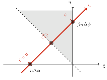
Figure 2: Illustration how to cut the $\xi$–$\eta$ plane in order to obtain the shape of the spectral lines as a function of $\ell$ for fixed scattering angle $\vartheta$.

Let us now return to our discussion of the properties of the master integrals Eq. (19) by first discussing how the rescaled arguments $\xi$ and $\eta$ relate to the frequency $\omega^{\prime}$ and scattering angle $\vartheta$ of the emitted photon. In order to obtain the shape of the frequency spectrum as a function of $\ell$ (or the photon frequency $\omega^{\prime}$ by means of Eq. (8)) one has to cut the functions $\mathcal{B}_{r}(\xi,\eta)$ along the straight line $\eta=\beta\xi+n\beta\Delta\phi$ in the $\xi$–$\eta$ plane, depicted as a red diagonal line in Fig. 2. This line intersects the $\xi$–axis at $\xi=-n\Delta\phi$, the slope is just $\beta$ (i.e. it depends on the laser intensity), and the intersection with the $\eta$–axis is at $\eta=\beta n\Delta\phi$. Note that the dependence on the scattering angle $\vartheta$ is entirely contained in the parameter $\beta$, see Eq. (10).

It is important to note which values of $\ell$ lie inside the grey shaded area where the master integrals are non-zero: They are exactly those values between the red-shifted and unshifted $n$-th harmonic lines in the infinite plane wave: $n/(1+\beta)\leq\ell\leq n$, see Fig. 2. Moreover, we see that the diagonal $\eta=-\xi$ represents the red-shifted harmonics in the infinite monochromatic plane wave. That means, the region close to the diagonal line $\eta=-\xi$ is formed close to the centre of the laser pulse where the intensity is largest. In the region close to the $\eta$–axis the master integrals is formed at the very edges of the laser pulse where the intensity is very low.

Numerical evaluations of the master integral $\mathcal{B}_{1}(\xi,\eta)$ are depicted in Fig. 3 for three different pulse envelopes. We see that each pulse shape generates a distinct pattern of oscillations in the triangular region bounded by the $\eta$–axis and the diagonal $\eta=-\xi$. For a Gaussian pulse envelope $g(t)=e^{-t^{2}/2}$ numerical evaluations of the master integrals are depicted in Fig. 4 for different values of $r$. One can see that the larger the value of $r$ the stronger the function is localized close to the line $\eta=-\xi$ (i.e. the non-linear Compton edge in the limit of infinite plane waves). By recalling how we need to cut the $\xi$–$\eta$ plane to obtain the frequency spectrum we easily deduce that for longer pulses or higher harmonics the spectral lines contain more oscillations. This observation is in line with results using the saddle point method (Seipt & Kämpfer, 2013b).

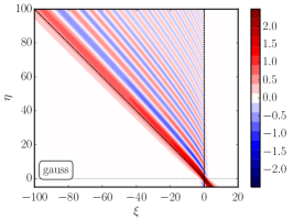
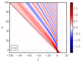
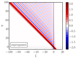
Figure 3: Numerical evaluation of the master integral $\mathcal{B}_{1}(\xi,\eta)$ for for different pulse shapes: a Gaussian $g(t)=e^{-t^{2}/2}$ (left), an exponential $g=e^{-|t|}$ (centre), and a Supergaussian $g=e^{-t^{4}/2}$ (right).

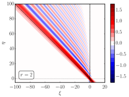
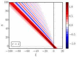
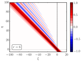
Figure 4: Numerical evaluation of the master integral (27) for a Gaussian pulse envelope $g=e^{-t^{2}/2}$ in the $\xi$–$\eta$ plane for increasing values of $r$ from left to right.

Before we conclude this paragraph, let us explicitly state how the rather abstract variables $\xi$ and $\eta$ are related to the physically observable photon frequency $\omega^{\prime}$ and scattering angle $\vartheta$. Those expressions explicitly read

$$\omega^{\prime}(\xi,\eta) =\frac{\xi+n\Delta\phi}{\Delta\phi+\frac{4\omega}{ma_{0}^{2}}\,\eta}\,,$$ (30)

$$\vartheta(\xi,\eta) =\arccos\left(\frac{4}{a_{0}^{2}}\frac{\eta}{\xi+n\Delta\phi}-1\right)\,.$$ (31)

By inspecting Fig. 2 together Eq. (10) we find that for any harmonic $n$ and any value of $r$, the physically relevant part of the master integral is located in a triangular region with the corner points $(\xi,\eta)=(0,0)$, $(0,n\Delta\phi\,a_{0}^{2}/2)$ and $(\xi_{0},-\xi_{0})$ with $\xi_{0}=n\Delta\phi\,a_{0}^{2}/(2+a_{0}^{2})$. That means for different $n$, pulse duration $\Delta\phi$ and $a_{0}$ different parts of the $\xi$–$\eta$ plane describe the spectrum of backscattered photons. The boundaries of these triangular regions are marked in Fig. 5 (left panel) for two different sets of parameters. When these areas are transformed to $\omega^{\prime}$ and $\vartheta$ we obtain the distributions in the centre and right panels, respectively. They strongly resemble the spectral line shapes in the incident electron rest frame found previously, e.g. in (Seipt & Kämpfer, 2013b).

For the sake of completeness, we also provide here the corresponding transformation relations in the laboratory frame where the electron counterpropagates the laser pulse with a Lorentz factor $\gamma$:

$$\omega^{\prime}_{\mathrm{lab}}(\xi,\eta) =\frac{\omega\gamma^{2}(1+v)^{2}(\xi+n\Delta\phi)}{\frac{1+v}{1-v+v\frac{4}{a_{0}^{2}}\frac{\eta}{\xi+n\Delta\phi}}\left(\Delta\phi+\frac{4}{a_{0}^{2}}\frac{\omega\gamma(1+v)\eta}{m}\right)}\,,$$ (32)

$$\vartheta_{\mathrm{lab}}(\xi,\eta) =\arccos\left(\frac{\frac{4}{a_{0}^{2}}\frac{\eta}{\xi+n\Delta\phi}-1+v}{1-v+v\frac{4}{a_{0}^{2}}\frac{\eta}{\xi+n\Delta\phi}}\right)\,,$$ (33)

where $v=\sqrt{1-1/\gamma^{2}}$. The differential on-axis photon emission probability in the laboratory frame, plotted in Fig. 6 for an initial electron energy of $51\text{\,}\mathrm{MeV}$ ($\gamma=100$) shows perfect agreement between a direct numerical evaluation of the dynamic integrals and the calculation of the master integrals and then transforming from the abstract $\xi$–$\eta$ plane to the photon frequency $\omega^{\prime}$ and $\vartheta=0$.

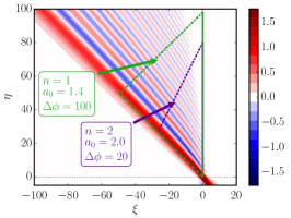
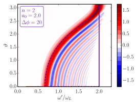
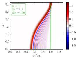
Figure 5: Transformation of the triangular regions in the $\xi$–$\eta$ plane to the variables $\omega^{\prime}$ and $\vartheta$. The solid, dashed and dash-dotted curves correspond to each other.

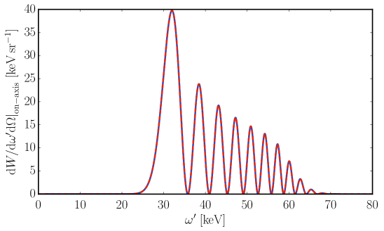
Figure 6: Differential on-axis photon emission probability in the laboratory frame for $a_{0}=1.5$, $\Delta\phi=25$, a Gaussian pulse shape and $\gamma=100$. The direct numerical evaluation of the dynamic integrals (blue solid) coincides perfectly with the evaluations of the master integrals (red dashed).

3.3 Universal Behaviour of High Order Harmonics

Let us now draw some conclusions about the shape of very high order harmonics. One can notice that for large values of $r$, the powers of $g^{r}(t)$ become strongly localized around $t\approx 0$. Thus, the main contribution to the master integral, Eq. (27), is provided by the region of $g(t)$ around the maximum at $t=0$. For sufficiently smooth pulse envelopes $g(t)$ a Taylor expansion around the point $t=0$ reads

$$g^{r}(t)\approx\left(1-|g^{\prime\prime}(0)|\frac{t^{2}}{2}\right)^{r}\,.$$ (34)

Defining $\tau^{2}=1/|g^{\prime\prime}(0)|$ and employing the known limit $(1+x/r)^{r}\stackrel{{\scriptstyle r\rightarrow\infty}}{{\to}}\,e^{x}$, we find

$$g^{r}(t)\approx e^{-\frac{r\,t^{2}}{2\tau^{2}}}\,.$$ (35)

which is of Gaussian shape and does not depend on any details of the primary pulse shape, except for the curvature at the maximum, i.e. the second derivative $g^{\prime\prime}(0)$ at $t=0$. Note that if one is concerned about laser pulses with a flat top envelope (in the sense that $g^{\prime\prime}(0)=0$), the Taylor series in (34) can be extended further, and will eventually lead to a Supergaussian shape of $g^{r}(t)$.

The conclusion is that for sufficiently high harmonic order the master integral is approximately given by

$$\mathcal{B}_{r}(\xi,\eta)\approx\intop_{-\infty}^{\infty}\!\mathrm{d}t\,e^{-\frac{r}{2}\left(\frac{t}{\tau}\right)^{2}+i\xi t+i\eta\int\!\mathrm{d}t\,g^{2}(t)}\,.$$ (36)

Because for large values of $r$ the main contributions to this integral come from a narrow region around $t=0$, we can approximate $\int dt\,g^{2}(t)$ polynomially around $t=0$ up to the third order. This allows us to give an analytic expression for the master integrals $\mathcal{B}_{r}$ for large values of $r\to\infty$ as

$$\mathcal{B}_{r}(\xi,\eta)\approx\frac{2\pi\tau^{2/3}}{\eta^{1/3}}\exp\left(-\frac{r}{2\eta}(\xi+\eta)+\frac{r^{3}}{12(\tau\eta)^{2}}\right)\operatorname{Ai}\left(\frac{r^{2}}{4(\tau\eta)^{4/3}}-\frac{\tau^{2/3}}{\eta^{1/3}}(\xi+\eta)\right)$$ (37)

in terms of the Airy function Ai (Erdélyi et al., 1953). The central conclusion here is that for very large values of $r$ the shape of the harmonic lines approximate the shape of the harmonics for a Gaussian laser pulse with temporal duration $\tau/\sqrt{r}=1/\sqrt{r|g^{\prime\prime}(0)|}$. The only specific input from the original pulse shape $g$ that affects the shape of the high-harmonic spectral lines is the curvature of the pulse envelope at the maximum.

3.4 Explicit Closed Form Analytic Results for the Master Integrals

We finally provide explicit closed form analytic expressions for the master integrals $\mathcal{B}_{r}(\xi,\eta)$ for several different laser pulse shapes $g$.

3.4.1 Hyperbolic Secant Pulse Shape

For a hyperbolic secant pulse, $g(t)=1/\cosh(t)$, we have $\int g^{2}dt=\tanh t$, and the master integral

$$\mathcal{B}_{r}(\xi,\eta) =\intop_{-\infty}^{\infty}\!\mathrm{d}t\,\frac{e^{i\xi t+i\eta\tanh t}}{\cosh^{r}t}$$ (38)

can be evaluated by transforming the integration variable according to $z=1/(2e^{t}\cosh t)$, yielding

$$\mathcal{B}_{r}(\xi,\eta) =2^{r-1}e^{-i\eta}\intop_{0}^{1}\!\mathrm{d}z\,\,z^{\frac{r+i\xi}{2}-1}(1-z)^{\frac{r-i\xi}{2}-1}\,e^{2i\eta z}\,.$$ (39)

This integral can be evaluated as

$$\mathcal{B}_{r}(\xi,\eta) =\frac{2^{r-1}e^{-i\eta}}{\Gamma(r)}\Gamma\left(\frac{r+i\xi}{2}\right)\Gamma\left(\frac{r-i\xi}{2}\right)\>_{1}F_{1}\left(\frac{r+i\xi}{2},r,2i\eta\right)\,,$$ (40)

with the Gamma function $\Gamma(z)$ and the confluent hyperbolic function ${}_{1}F_{1}(a,b;z)$ (Erdélyi et al., 1953). An equivalent representation of (40) can be given in terms of the generalized Laguerre functions $\mathcal{L}^{\lambda}_{\nu}(z)$ (Erdélyi et al., 1953) as

$$\mathcal{B}_{r}(\xi,\eta) =\frac{2^{r-1}e^{-i\eta}\pi}{\sin\left(\frac{\pi}{2}(r+i\xi)\right)}\mathcal{L}^{r-1}_{-\frac{r+i\xi}{2}}(2i\eta)\,.$$ (41)

3.4.2 Exponential Pulse Shape

For a pulse shape of the form $g(t)=e^{-|t|}$ the master integral takes the form

$$\mathcal{B}_{r}(\xi,\eta) =\intop_{0}^{\infty}\!\mathrm{d}t\,e^{-(r-i\xi)t}\,e^{i\eta e^{-t}\sinh t}\>+\>\rm c.c.\,.$$ (42)

After a substitution $z=\frac{i\eta}{2}e^{-2t}$ we get

$$\mathcal{B}_{r}(\xi,\eta) =\frac{e^{\frac{i\eta}{2}}}{2}\left(\frac{2}{i\eta}\right)^{\frac{r-i\xi}{2}}\intop_{0}^{\frac{i\eta}{2}}\!\mathrm{d}z\,z^{\frac{r-i\xi}{2}-1}\,e^{-z}\>+\>\rm c.c.\,,$$ (43)

which can be expressed as

$$\mathcal{B}_{r}(\xi,\eta) =\frac{e^{i\eta/2}}{2}\left(\frac{2}{i\eta}\right)^{\frac{r-i\xi}{2}}\gamma\left(\frac{r-i\xi}{2},\frac{i\eta}{2}\right)\>+\>\rm c.c.\,,$$ (44)

with the lower incomplete gamma function $\gamma(a,z)$ (Erdélyi et al., 1953),

3.4.3 Staircase Pulse Shapes

Let us assume the pulse envelope is staircase, defined as $g(t)=\sum_{k=1}^{N}\nu_{k}\chi_{I_{k}}(t)$ for $t>0$, with $\nu_{k}$ being the height of the $k$-th step (as measured from the ground level) and the characteristic function $\chi_{I_{k}}(t)=1$ if $t\in I_{k}=[(k-1)/N,k/N)$, and zero otherwise. (For $t<0$ the envelope is fully defined by the symmetry $g(-t)=g(t)$.) For the moment we assume that the step height increases uniformly, $\nu_{k}=(N-k+1)/N$, but a generalization to arbitrary steps is obvious. A compelling feature of the staircase pulse is the possibility to approximate many different smooth pulse shapes in the limit of infinite steps $N\to\infty$, just by adjusting the step heights. For instance, the uniform staircase discussed here would converge to a smooth triangle pulse.

By splitting the $t$-integration range into the intervals $I_{k}$ where $g$ is constant we evaluate the master integral as

$$\mathcal{B}_{r}(\xi,\eta) =\sum_{k=1}^{N}2(\nu_{k})^{r}\>\frac{\sin\frac{\xi+\eta\,\nu^{2}_{k}}{2}}{\frac{\xi+\eta\,\nu^{2}_{k}}{2}}\>\cos\left(\eta\,\Phi_{k}+\frac{2k-1}{N}\frac{\xi+\eta\,\nu^{2}_{k}}{2}\right)$$ (45)

with

$$\Phi_{k}=\frac{1}{N}\sum_{\kappa=1}^{k}\nu_{\kappa}^{2}-\frac{k}{N}\nu_{k}^{2}\,.$$ (46)

For $N=1$ we recover the well known result of of a sinc profile for the box pulse which is aligned along the $\eta=-\xi$ diagonal, i.e. it corresponds to the usual infinite plane wave red-shift. While the bandwidth of the laser pulse translates to the Compton scattered light, we see no indication of the ponderomotive broadening due to a gradual ramp up of the laser intensity. How this ponderomotive broadening effect develops can be seen quite instructively when going to a pulse with more than one step. For $N$ steps we observe a total of $N$ strips in the $\eta$–$\xi$ plane that are centred along the lines $\eta=-\xi/\nu_{k}^{2}$. On each of the steps the radiation is emitted with with their respective red-shift, determined by the square of the $k$-th step height as $\ell=n/(1+\beta\nu_{k}^{2})$. With increasing $N$ these strips eventually are overlapping, reproducing the typical picture from the smooth pulses discussed before. Thus, the staircase pulse model discussed here helps to investigate the transition from the case of a constant amplitude laser pulse to the case of smooth pulses where the ponderomotive broadening sets in and strongly influences the non-linear Compton spectrum.

4 Conclusions

In summary, we provided in this paper a comprehensive and completely analytical evaluation of the non-linear Compton transition amplitude. It was found that the dependence on the shape of the strong laser pulse can be traced back to a class of three-parameter master integrals. In addition, all the dependence on the pulse duration can be conveniently scaled out from the master integral. For certain shapes of the laser pulse envelope we provided explicit analytical expressions for the master integrals. In addition, for very high harmonics we find a universal behaviour of the shape of the harmonic lines.

In this paper we studied only the case of circularly polarized laser light. The laser polarization affects the form of the Jacobi-Anger type expansion (13) and the subsequent extraction of the laser pulse envelope from the argument of the Bessel functions via Eq. (16). In the case of an elliptic or linear laser polarization we would encounter generalized two-argument Bessel functions (Seipt, 2012; Korsch et al., 2006). But eventually the laser pulse shape dependence is described by exactly the same master integrals (19) as for circular laser polarization discussed in this paper.

We would like to stress that the analytical structure of the strong-field $S$ matrix is similar also for other first-order strong-field QED processes like Breit-Wheeler pair production, or pair annihilation. Thus, our analytic results could be easily translated to these processes too.

Acknowledgments

This work was supported in part by the Helmholtz Association (Helmholtz Young Investigators group VH-NG-1037).

References

- Berestetzki et al. (1980) Berestetzki, W. B., Lifschitz, E. M. & Pitajewski, L. P. 1980 Relativistische Quantentheorie, Lehrbuch der Theoretischen Physik, vol. IV. Berlin: Akademie Verlag.
- Boca & Florescu (2009) Boca, M. & Florescu, V. 2009 Nonlinear compton scattering with a laser pulse. Phys. Rev. A 80, 053403.
- Brown & Kibble (1964) Brown, L. S. & Kibble, T. W. B. 1964 Interaction of intense laser beams with electrons. Phys. Rev. 133, A705.
- Di Piazza et al. (2012) Di Piazza, A., Müller, C., Hatsagortsyan, K. Z. & Keitel, C. H. 2012 Extremely high-intensity laser interactions with fundamental quantum systems. Rev. Mod. Phys. 84, 1177.
- Dinu (2013) Dinu, V. 2013 Exact final state integrals for strong field QED. Phys. Rev. A 87, 052101, arXiv:1302.1513 [hep-ph].
- Dinu et al. (2015) Dinu, V., Harvey, C., Ilderton, A., Marklund, M. & Torgrimsson, G. 2015 Quantum radiation reaction: from interference to incoherence. ArXiv:1512.04096 [hep-ph].
- Erdélyi et al. (1953) Erdélyi, A., Magnus, W., Oberhettinger, F. & Tricomi, F. G. 1953 Higher Transcendental Functions. McGraw-Hill.
- Fedotov et al. (2010) Fedotov, A. M., Narozhny, N. B., Mourou, G. & Korn, G. 2010 Limitations on the attainable intensity of high power lasers. Phys. Rev. Lett. 105, 080402.
- Goldman (1964) Goldman, I. I. 1964 Intensity effects in compton scattering. Phys. Lett. 8, 103.
- Hartemann et al. (2010) Hartemann, Frederic V., Albert, Félice, Siders, Craig W. & Barty, C. P. J. 2010 Low-intensity nonlinear sprectral effects in compton scattering. Phys. Rev. Lett. 105, 130801.
- Hartemann & Kerman (1996) Hartemann, F. V. & Kerman, A. K. 1996 Classical theory of nonlinear compton scattering. Phys. Rev. Lett. 76, 624.
- Hartemann et al. (1996) Hartemann, F. V., Troha, A. L., Luhmann Jr., N. C. & Toffano, Z. 1996 Spectral analysis of the nonlinear relativistic doppler shift in ultrahigh intensity compton scattering. Phys. Rev. E 54, 2956.
- Harvey et al. (2009) Harvey, Chris, Heinzl, Thomas & Ilderton, Anton 2009 Signatures of High-Intensity Compton Scattering. Phys. Rev. A 79, 063407.
- Harvey et al. (2015) Harvey, C. N., Ilderton, A. & King, B. 2015 Testing numerical implementations of strong field electrodynamics. Phys. Rev. A 91 (1), 013822, arXiv:1409.6187.
- Ilderton (2011) Ilderton, A. 2011 Trident pair production in strong laser pulses. Phys. Rev. Lett. 106, 020404, arXiv: arxiv:1011.4072.
- Jochmann et al. (2013) Jochmann, A. & others 2013 High resolution energy-angle correlation measurement of hard x rays from laser-thomson backscattering. Phys. Rev. Lett. 111, 114803.
- Khrennikov et al. (2015) Khrennikov, K., Wenz, J., Buck, A., Xu, J., Heigoldt, M., Veisz, L. & Karsch, S. 2015 Tunable all-optical quasimonochromatic thomson x-ray source in the nonlinear regime. Phys. Rev. Lett. 114, 195003, arXiv:1406.6654 [physics.plasm-ph].
- King et al. (2013) King, B., Elkina, N. & Ruhl, H. 2013 Photon polarization in electron-seeded pair-creation cascades. Phys. Rev. A 87, 042117.
- Korsch et al. (2006) Korsch, H. J., Klumpp, A. & Witthaut, D. 2006 On two-dimensional bessel functions. J. Phys. A 39, 14947–14964.
- Korzhimanov et al. (2011) Korzhimanov, A. V., Gonoskov, A. A., Khazanov, E. A. & Sergeev, A. M. 2011 Horizons of petawatt laser technology. Phys. Usp. 54, 9.
- Krajewska & Kamiński (2012) Krajewska, K. & Kamiński, J. Z. 2012 Compton process in intense short laser pulses. Phys. Rev. A 85, 062102.
- Mackenroth & Di Piazza (2011) Mackenroth, F. & Di Piazza, A. 2011 Nonlinear compton scattering in ultra-short laser pulses. Phys. Rev. A 83, 032106, arXiv: arXiv:1010.6251 hep-ph.
- Mackenroth et al. (2010) Mackenroth, F., Di Piazza, A. & Keitel, C. H. 2010 Determining the Carrier-Envelope phase of intense Few-Cycle laser pulses. Phys. Rev. Lett. 105 (6), 063903.
- Mourou et al. (2006) Mourou, Gerard A., Tajima, Toshiki & Bulanov, Sergei V. 2006 Optics in the relativistic regime. Rev. Mod. Phys. 78 (2), 309–371.
- Narozhny & Fedotov (2015) Narozhny, N. B. & Fedotov, A. M. 2015 Quantum-electrodynamic cascades in intense laser fields. Uspekhi Fizicheskikh Nauk 185 (1), 103.
- Narozhnyi & Fofanov (1996) Narozhnyi, N. B. & Fofanov, M. S. 1996 Photon emission by an electron in a collision with a short focused laser pulse. J. Exp. Theor. Phys. 83, 14.
- Nikishov & Ritus (1964a) Nikishov, A. I. & Ritus, V. I. 1964a Quantum processes in the field of a plane electromagnetic wave and in a constant field. Sov. Phys. J. Exp. Theor. Phys. 19, 1191.
- Nikishov & Ritus (1964b) Nikishov, A. I. & Ritus, V. I. 1964b Quantum processes in the field of a plane electromagnetic wave and in a constant field. I. Sov. Phys. J. Exp. Theor. Phys. 19, 529.
- Nikishov & Ritus (1965) Nikishov, A. I. & Ritus, V. I. 1965 Nonlinear effects in compton scattering and pair production owing to absorption of several photons. Sov. Phys. J. Exp. Theor. Phys. 20, 757.
- Ritus (1985) Ritus, V. I. 1985 Quantum effects of the interaction of elementary particles with an intense electromagnetic field. J. Sov. Laser Res. 6, 497.
- Rykovanov et al. (2014) Rykovanov, S. G., Geddes, C. G. R., Vay, J.-L., Schroeder, C. B., Esarey, E. & Leemans, W. P. 2014 Quasi-monoenergetic femtosecond photon sources from thomson scattering using laser plasma accelerators and plasma channels. J. Phys. B 47 (23), 234013, arXiv:1406.1832 [physics.plasm-ph].
- Sarri et al. (2014) Sarri, G., Corvan, D. J., Schumaker, W., Cole, J. M., Di Piazza, A., Ahmed, H., Harvey, C., Keitel, C. H., Krushelnick, K., Mangles, S. P. D., Najmudin, Z., Symes, D., Thomas, A. G. R., Yeung, M., Zhao, Z. & Zepf, M. 2014 Ultrahigh brilliance multi-mev -ray beams from nonlinear relativistic Thomson scattering. Phys. Rev. Lett. 113, 224801.
- Seipt (2012) Seipt, Daniel 2012 Strong field QED processes in short laser pulses. PhD thesis, Technische Universität Dresden.
- Seipt & Kämpfer (2011) Seipt, D. & Kämpfer, B. 2011 Non-linear compton scattering of ultrashort and intense laser pulses. Phys. Rev. A 83, 022101.
- Seipt & Kämpfer (2013a) Seipt, D. & Kämpfer, B. 2013a Asymmetries of azimuthal photon distributions in nonlinear compton scattering in ultrashort intense laser pulses. Phys. Rev. A 88, 012127.
- Seipt & Kämpfer (2013b) Seipt, D. & Kämpfer, B. 2013b Non-linear compton scattering of ultrahigh-intensity laser pulses. Laser Phys. 23 (7), 075301, seipt:2011; arXiv:1111.0188v1 [hep-ph].
- Seipt et al. (2015a) Seipt, D., Rykovanov, S. G., Surzhykov, A. & Fritzsche, S. 2015a Narrowband inverse Compton scattering x-ray sources at high laser intensities. Phys. Rev. A 91, 033402.
- Seipt et al. (2015b) Seipt, D., Surzhykov, A., Fritzsche, S. & Kämpfer, B. 2015b Caustic structures in the spectrum of x-ray compton scattering off electrons driven by a short intense laser pulse. ArXiv:1507.08868 [hep-ph].
- Twardy et al. (2014) Twardy, M., Krajewska, K. & Kamiński, J. Z. 2014 Shape effects in nonlinear thomson and compton processes. J. Phys. Conf. Ser. 497, 012019.
- Watson (1922) Watson, G. N. 1922 A treatise on the theory of Bessel functions. Cambridge University Press.