Comparing magic wavelengths for the $6s~{}{{}^{2}}S_{1/2}-6p~{}{{}^{2}}P_{1/2,3/2}$ transitions of Cs using circularly and linearly polarized light

Abstract

We demonstrate magic wavelengths, at which external electric field produces null differential Stark shifts, for the $6s~{}{{}^{2}}S_{1/2}-6p~{}{{}^{2}}P_{1/2,3/2}$ transitions in the Cs atom due to circularly polarized light. In addition, we also obtain magic wavelengths using linearly polarized light, in order to verify the previously reported values, and make a comparative study with the values obtained for circularly polarized light. A number of these wavelengths are found to be in the optical region and could be of immense interest to experimentalists for carrying out high precision measurements. To obtain these wavelengths, we have calculated dynamic dipole polarizabilities of the ground, $6p~{}{{}^{2}}P_{1/2}$ and $6p~{}{{}^{2}}P_{3/2}$ states of Cs. We use the available precise values of the electric dipole (E1) matrix elements of the transitions that give the dominant contributions from the lifetime measurements of the excited states. Other significantly contributing E1 matrix elements are obtained by employing a relativistic coupled-cluster singles and doubles method. The accuracies of the dynamic polarizabilities are substantiated by comparing the static polarizability values with the corresponding experimental results.

I Introduction

Techniques involving laser cooling and trapping of neutral atoms are of immense interest for many scientific applications, including those that are capable of probing new physics phillip and searching for exotic quantum phase transitions using ultracold atoms  grim . In particular, trapping atoms using optical lattices have many advantages since they offer long storage time  grim ; balykin ; sahoo1 and their energy levels can be easily accessed using lasers adams . It is conducive to carry out measurements in a transition of an optically trapped atom without realizing the Stark shifts due to the applied laser field. One can achieve this by trapping the atom at the wavelengths for which the differential Stark shift of the transition gets nullified. These wavelengths are popularly known as magic wavelengths (${\rm\lambda_{magic}}$s)  katori . They play crucial role in state-insensitive quantum engineering to set-up many high precision experiments. They are useful in the atomic clock experiments to acquire relative uncertainty as small as $\sim\rm 10^{-18}$  porto ; sac ; sahoo1 , in the quantum information and communication studies Monroe , investigating fundamental physics fortier ; Weiss , so on.

Alkali atoms are mostly preferred for performing experiments using laser cooling and trapping techniques. The reason being that the low-lying transitions in these atoms are conveniently accessible by the available lasers. Since Cs atom has wider hyperfine splittings in its ground state, it has been considered for making microwave clock and for quantum computation. For laser cooling of these atoms, its $6s~{}{{}^{2}}S_{1/2}$-$6p~{}{{}^{2}}P_{3/2}$ transitions are mainly being used. Owing to a large number of applications of trapped Cs atoms, it would be imperative to find out all plausible magic wavelengths of these transitions such that lasers can be appropriately chosen at these wavelengths to reduce systematics significantly in the above possible measurements due to the Stark shifts. Mckeever et al. had experimentally demonstrated ${\rm\lambda_{magic}}$ at 935.6 nm for the $6s~{}{{}^{2}}S_{1/2}$-$6p~{}{{}^{2}}P_{3/2}$ transition in Cs mck using linearly polarized light. Following this, magic wavelengths for many alkali atoms including Cs atom were determined using linearly polarized light by Arora et al. arora1 by evaluating the dynamic polarizabilities of these atoms using the relativistic coupled cluster (RCC) method. The estimation of ac Stark shifts using circularly polarized light may be advantageous to look for magic wavelengths owing to the predominant role played by the vector polarizabilities. Since the vector polarizability contribution is absent in the use of linearly polarized light, this can open-up new windows to manipulate the magic wavelengths for a wide range of applications. Recently, we had investigated magic wavelengths in the lighter alkali atoms for circularly polarized light and realized many possible magic wavelengths, especially for the $ns~{}{{}^{2}}S_{1/2}$-$np~{}{{}^{2}}P_{3/2}$ transitions with the ground state principal quantum number $n$ sahoo1 ; arorab ; arora2 . However, magic wavelengths for circularly polarized light in the Cs atom have not been explored sufficiently.

Table 1: Contributions from different E1 matrix elements ($d$) to the static polarizabilities of the $6S_{1/2}$, $6P_{1/2}$ and $6P_{3/2}$ states of Cs atom. The final results are compared with the previously estimated and available experimental results. Uncertainties are given in the parentheses.

$6S_{1/2}$ state			$6P_{1/2}$ state			$6P_{3/2}$ state
Transition	$d$	$\alpha^{(0)}$	Transition	$d$	$\alpha^{(0)}$	Transition	$d$	$\alpha^{(0)}$	$\alpha^{(2)}$
$6S_{1/2}-6P_{1/2}$	4.489(7)	131.88(2)	$6P_{1/2}-6S_{1/2}$	4.489(7)	-131.88(2)	$6P_{3/2}-6S_{1/2}$	6.324(7)	-124.69(2)	124.69(2)
$6S_{1/2}-7P_{1/2}$	0.30(3)	0.30	$6P_{1/2}-7S_{1/2}$	4.236(21)	178.43(7)	$6P_{3/2}-7S_{1/2}$	6.47(3)	225.3(1)	-225.3(1)
$6S_{1/2}-8P_{1/2}$	0.09(1)	0.02	$6P_{1/2}-8S_{1/2}$	1.0(1)	5.86(1)	$6P_{3/2}-8S_{1/2}$	1.5(1)	6.21(2)	-6.21(2)
$6S_{1/2}-9P_{1/2}$	0.04	$\sim$0	$6P_{1/2}-9S_{1/2}$	0.55(6)	1.41	$6P_{3/2}-9S_{1/2}$	0.77(8)	1.44	-1.44
$6S_{1/2}-10P_{1/2}$	0.02	$\sim$0	$6P_{1/2}-10S_{1/2}$	0.36(4)	0.57	$6P_{3/2}-10S_{1/2}$	0.51(5)	0.57	-0.57
$6S_{1/2}-11P_{1/2}$	0.02	$\sim$0	$6P_{1/2}-11S_{1/2}$	0.27(3)	0.29	$6P_{3/2}-11S_{1/2}$	0.37(4)	0.29	-0.29
$6S_{1/2}-12P_{1/2}$	0.01	$\sim$0	$6P_{1/2}-12S_{1/2}$	0.20(2)	0.17	$6P_{3/2}-12S_{1/2}$	0.29(3)	0.17	-0.17
$6S_{1/2}-6P_{3/2}$	6.324(7)	249.38(3)	$6P_{1/2}-5D_{3/2}$	7.016(24)	1084.3(5)	$6P_{3/2}-5D_{3/2}$	3.166(16)	132.51(4)	106.01(3)
$6S_{1/2}-7P_{3/2}$	0.60(6)	1.20	$6P_{1/2}-6D_{3/2}$	4.3(4)	120.98(9)	$6P_{3/2}-6D_{3/2}$	2.1(2)	15.54(7)	12.43(5)
$6S_{1/2}-8P_{3/2}$	0.23(2)	0.15	$6P_{1/2}-7D_{3/2}$	2.1(2)	21.03(8)	$6P_{3/2}-7D_{3/2}$	1.0(1)	2.47	1.97
$6S_{1/2}-9P_{3/2}$	0.13(1)	0.05	$6P_{1/2}-8D_{3/2}$	1.3(1)	7.43(1)	$6P_{3/2}-8D_{3/2}$	0.61(6)	0.84	0.67
$6S_{1/2}-10P_{3/2}$	0.09(1)	0.02	$6P_{1/2}-9D_{3/2}$	0.93(9)	3.55	$6P_{3/2}-9D_{3/2}$	0.43(4)	0.40	0.32
$6S_{1/2}-11P_{3/2}$	0.06(1)	0.01	$6P_{1/2}-10D_{3/2}$	0.71(7)	2.01	$6P_{3/2}-10D_{3/2}$	0.33(3)	0.22	0.18
$6S_{1/2}-12P_{3/2}$	0.05	0.01				$6P_{3/2}-5D_{5/2}$	9.59(8)	1174(2)	-234.9(4)
						$6P_{3/2}-6D_{5/2}$	6.3(6)	132(2)	-26.4(3)
						$6P_{3/2}-7D_{5/2}$	2.9(3)	21.6(1)	-4.32(3)
						$6P_{3/2}-8D_{5/2}$	1.8(2)	7.46(3)	-1.49
						$6P_{3/2}-9D_{5/2}$	1.3(1)	3.53	-0.71
						$6P_{3/2}-10D_{5/2}$	1.0(1)	1.98	-0.40
Main($\rm\alpha_{v}^{v}$)		383.03(4)	Main($\rm\alpha_{v}^{v}$)		1294.2(5)	Main($\rm\alpha_{v}^{v}$)		1602(3)	-255.9(5)
Tail($\rm\alpha_{v}^{v}$)		0.15(8)	Tail($\rm\alpha_{v}^{v}$)		24(12)	Tail($\rm\alpha_{v}^{v}$)		25(13)	-5(2)
$\rm\alpha_{v}^{cv}$		-0.47(0)	$\rm\alpha_{v}^{cv}$		$\sim$0	$\rm\alpha_{v}^{cv}$		$\sim$0	$\sim 0$
$\rm\alpha_{0}^{c}$		16.8(8)	$\rm\alpha_{0}^{c}$		16.8(8)	$\rm\alpha_{0}^{c}$		16.8(8)
Total		399.5(8)	Total		1335(12)	Total		1644(13)	-261(2)
Others		399.9derevianko	Others		1338arora1	Others		1650arora1	-261arora1
		399borschevsky			1290wijngaarden			1600wijngaarden	-233 wijngaarden
Experiment		401.0(6)amini	Experiment		1328.4(6)hunter	Experiment		1641(2)tanner	-262(2)tanner

In this paper, we determine the magic wavelengths for the 6$s~{}{{}^{2}}S_{1/2}$-6$p~{}{{}^{2}}P_{1/2,3/2}$ transitions in the Cs atom using circularly polarized light. For this purpose, we calculate the dipole polarizabilities of the ground, $6p~{}{{}^{2}}P_{1/2}$ and $6p~{}{{}^{2}}P_{3/2}$ states very precisely. The static polarizability values are compared with the experimental results to verify accuracies in our results. We also determine magic wavelengths due to linearly polarized light for the 6$s~{}{{}^{2}}S_{1/2}$-6$p~{}{{}^{2}}P_{1/2,3/2}$ transitions using these polarizabilities and compare with the previously reported values in order to validate our approach. We have used atomic unit (a.u.), unless stated otherwise.

II Theory and Method of Evaluation

In the time independent second order perturbation theory, the Stark shift in the energy of $v^{th}$ level of an atom placed in a static electric field ($\cal E$) is expressed as bonin

$$\Delta E_{v}=\sum_{k\neq v}\frac{|\langle\psi_{v}|V|\psi_{k}\rangle|^{2}}{E_{v}^{0}-E_{k}^{0}},$$ (1)

where $V=-\mbox{\boldmath$D$}\cdot\mbox{\boldmath$\cal E$}$ is the perturbing electric-dipole interaction Hamiltonian, $E_{i}^{0}$ refers to the unperturbed energy of the corresponding level denoted by $i=k,v$ and states with subscript $k$ are the intermediate states to which transition from the $v^{th}$ state is allowed by the dipole selection rules. For convenience, Eq. (1) is simplified to get

$$\Delta E_{v}=-\frac{1}{2}\alpha_{v}{\cal E}^{2},$$ (2)

where, $\alpha_{v}$ is the static dipole polarizability, and is given by

$$\alpha_{v}=-2\sum_{k\neq v}\frac{(p^{*})_{vk}(p)_{kv}}{\delta E_{vk}}.$$ (3)

Here, $\delta E_{vk}=E_{v}^{0}-E_{k}^{0}$ and $(p)_{kv}=\langle\psi_{k}|D|\psi_{v}\rangle$ is the electric dipole (E1) matrix element between the states $|\psi_{v}\rangle$ and $|\psi_{k}\rangle$. Since in a number of applications, oscillating electric fields are used, the above expression is slightly modified for that case, with polarizability as a function of frequency of the electric field, asmanakov

$$\alpha_{v}(\omega)=-\sum_{k\neq v}{(p^{*})_{vk}(p)_{kv}}\left[\frac{1}{\delta E_{vk}+\omega}+\frac{1}{\delta E_{vk}-\omega}\right].$$ (4)

For circularly polarized light, in the absence of magnetic field, the above expression is further parameterized in terms of ranks 0, 1 and 2 components of the tensor products that are known as scalar ($\rm\alpha_{v}^{(0)}$), vector ($\rm\alpha_{v}^{(1)}$) and tensor ($\rm\alpha_{v}^{(2)}$) polarizabilities respectively i.e.

$$\alpha_{v}(\omega)=\alpha_{v}^{(0)}+\frac{Am_{j}}{2j_{v}}\alpha_{v}^{(1)}-\frac{3m_{j}^{2}-j_{v}(j_{v}+1)}{2j_{v}(2j_{v}-1)}\alpha_{v}^{(2)},$$ (5)

where $j_{v}$ is the angular momentum, $m_{j}$ is its magnetic projection, and

$$\alpha_{v}^{(0)} = \frac{1}{3(2j_{v}+1)}\sum_{j_{k}}|\langle j_{v}||D||j_{k}\rangle|^{2}$$ (6)

$$\times\left[\frac{1}{\delta E_{kv}+\omega}+\frac{1}{\delta E_{kv}-\omega}\right],$$

$$\alpha_{v}^{(1)} = -\sqrt{\frac{6j_{v}}{(j_{v}+1)(2j_{v}+1)}}\sum_{j_{k}}(-1)^{j_{k}+j_{v}+1}$$ (10)

$$\times\left\{\begin{array}[]{ccc}j_{v}&1&j_{v}\\ 1&j_{k}&1\end{array}\right\}|\langle j_{v}||D||j_{k}\rangle|^{2}$$

$$\times\left[\frac{1}{\delta E_{kv}+\omega}-\frac{1}{\delta E_{kv}-\omega}\right]$$

and

$$\alpha_{v}^{(2)} = -2\sqrt{\frac{5j_{v}(2j_{v}-1)}{6(j_{v}+1)(2j_{v}+3)(2j_{v}+1)}}$$ (14)

$$\times\sum_{j_{k}}(-1)^{j_{k}+j_{v}+1}\left\{\begin{array}[]{ccc}j_{v}&2&j_{v}\\ 1&j_{k}&1\end{array}\right\}|\langle j_{v}||D||j_{k}\rangle|^{2}$$

$$\times\left[\frac{1}{\delta E_{kv}+\omega}+\frac{1}{\delta E_{kv}-\omega}\right],$$

for the reduced matrix element $|\langle j_{v}||D||j_{k}\rangle|$ with the angular momentum $j_{k}$ of the intermediate state $k$. Here, $A$ is the degree of circular polarization assuming the quantization axis to be in the direction of wave vector and possess values $1$ and $-1$ for the right handed and left handed circularly polarized light, respectively. The expressions denoted within curly brackets are the angular momentum coupling 6-j symbols edmonds .

For linearly polarized light, “the degree of circular polarization $A=0$”. and total frequency dependent polarizability in this case can be formulated as

$$\alpha_{v}(\omega)=\alpha_{v}^{(0)}+\frac{3m_{j}^{2}-j_{v}(j_{v}+1)}{j_{v}(2j_{v}-1)}\alpha_{v}^{(2)},$$ (15)

where we assume the quantization axis along the direction of polarization vector.

Figure 1: (Color online) Dynamic polarizabilities (in a.u.) for the $6S_{1/2}$ and $6P_{1/2}$ states of Cs with different $m_{j}$ values in the wavelength range 600-770 nm for linearly polarized light (upper half) and circularly polarized light (lower half).

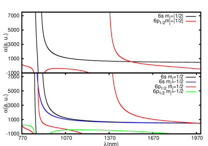
Figure 2: (Color online) Dynamic polarizabilities (in a.u.) for the $6S_{1/2}$ and $6P_{1/2}$ states in Cs with different $m_{j}$ values in the wavelength range 770-2000 nm for linearly polarized light (upper half) and circularly polarized light (lower half).

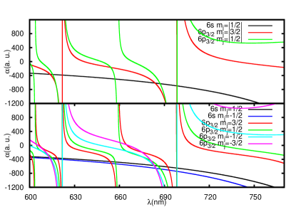
Figure 3: (Color online) Dynamic polarizabilities (in a.u.) of the $6S_{1/2}$ and $6P_{3/2}$ states in Cs with different $m_{j}$ values in the wavelength range 600-770 nm for linearly polarized light (upper half) and circularly polarized light (lower half).

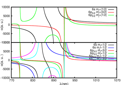
Figure 4: (Color online) Dynamic polarizabilities (in a.u.) of the $6S_{1/2}$ and $6P_{3/2}$ states in Cs with different $m_{j}$ values in the wavelength range 770-1070 nm for linearly polarized light (upper half) and circularly polarized light (lower half).

Table 2: Magic wavelengths ($\lambda_{\rm{magic}}$s) (in nm) with corresponding polarizabilities ($\alpha_{v}(\omega)$s) (in a.u.) for the $6S-6P_{1/2}$ transition in the Cs atom with linearly and circularly polarized light along with the resonant wavelengths ($\lambda_{\rm{res}}$s) (in nm).

		Linearly Polarization				Circularly Polarization
		Present		Ref.arora1		Transition: $6S(m_{j}=1/2)-6P_{1/2}$				Transition: $6S(m_{j}=-1/2)-6P_{1/2}$
		$m_{j}=|1/2|$				$m_{j}=1/2$		$m_{j}=-1/2$		$m_{j}=1/2$		$m_{j}=-1/2$
Resonance	$\lambda_{\rm{res}}$	$\lambda_{\rm{magic}}$	$\alpha_{v}(\omega)$	$\lambda_{\rm{magic}}$	$\alpha_{v}(\omega)$	$\lambda_{\rm{magic}}$	$\alpha_{v}(\omega)$	$\lambda_{\rm{magic}}$	$\alpha_{v}(\omega)$	$\lambda_{\rm{magic}}$	$\alpha_{v}(\omega)$	$\lambda_{\rm{magic}}$	$\alpha_{v}(\omega)$
$6P_{1/2}-8D_{3/2}$	601.22
		634.3(2)	-424	634.3(2)	-424(2)	632.0(6)	-398			632.4(4)	-437
$6P_{1/2}-9S_{1/2}$	635.63
		659.8(8)	-511	660.1(6)	-513(3)	663.4(8)	-497	656.4(8)	-473	664.6(6)	-559	657.7(7)	-530
$6P_{1/2}-7D_{3/2}$	672.51
		759.38(5)	-1282	759.40(3)	-1282(3)	756.1(1)	-1104			757.25(8)	-1381
$6P_{1/2}-8S_{1/2}$	761.10
$6P_{1/2}-6D_{3/2}$	876.38
										880.79(8)	5907
$6P_{1/2}-6S_{1/2}$	894.59
$6P_{1/2}-7S_{1/2}$	1359.20
		1522(3)	582	1520(3)	583(2)	1966(10)	500			1981(10)	480
$6P_{1/2}-5D_{3/2}$	3011.15

The differential ac Stark shift of a transition between the ground state and an excited state is the difference between the ac Stark shifts of the two states and is given by

$$\delta(\Delta E)_{ge}(\omega) = \Delta E_{g}(\omega)-\Delta E_{e}(\omega)$$ (16)

$$= -\frac{1}{2}\left[\alpha_{g}(\omega)-\alpha_{e}(\omega)\right]{\cal E}^{2}.$$

Here, subscripts ‘$g$’ and ‘$e$’ represent the ground and excited states, respectively. Our aim is to find out the $\omega$ values at which $\delta(\Delta E)_{ge}(\omega)$ will be zero.

Table 3: Magic wavelengths ($\lambda_{\rm{magic}}$s) (in nm) with corresponding polarizabilities ($\alpha_{v}(\omega)$s) (in a.u.) for the $6S-6P_{3/2}$ transition in the Cs atom with linearly polarized light along with the resonant wavelengths ($\lambda_{\rm{res}}$s) (in nm).

Transition		$m_{j}=|1/2|$				$m_{j}=|3/2|$
$6S(m_{j}=|1/2|)-6P_{3/2}$		Present		Ref. arora1		Present		Ref. arora1
Resonance	$\lambda_{\rm{res}}$	$\lambda_{\rm{magic}}$	$\alpha_{v}(\omega)$	$\lambda_{\rm{magic}}$	$\alpha_{v}(\omega)$	$\lambda_{\rm{magic}}$	$\alpha_{v}(\omega)$	$\lambda_{\rm{magic}}$	$\alpha_{v}(\omega)$
$6P_{3/2}-9D_{5/2}$	584.68
		602.6(3)	-338	602.6(4)	-339(1)
$6P_{3/2}-10S_{1/2}$	603.58
		615.4(10)	-370	615.5(8)	-371(3)	614(1)	-365	614(3)	-367(8)
$6P_{3/2}-8D_{5/2}$	621.48
		621.924(4)	-387	621.924(2)	-388(1)	621.85(4)	-387	621.844(3)	-388(1)
$6P_{3/2}-8D_{3/2}$	621.93
		657.0(2)	-500	657.05(9)	-500(1)
$6P_{3/2}-9S_{1/2}$	658.83
		687(1)	-633	687.3(3)	-635(3)	684(1)	-617	684.1(5)	-618(4)
$6P_{3/2}-7D_{5/2}$	697.52
		698.5(5)	-697	698.524(2)	-697(2)	698.3(7)	-695	698.346(4)	-696(2)
$6P_{3/2}-7D_{3/2}$	698.54
		793.1(2)	-2072	793.07(2)	-2074(5)
$6P_{3/2}-8S_{1/2}$	794.61
$6S_{1/2}-6P_{3/2}$	852.35
		888(2)	-5690	887.95(10)	-5600(100)	884(3)	-1618	883.4(2)	-1550(90)
$6S_{1/2}-6P_{1/2}$	894.59
$6P_{3/2}-6D_{5/2}$	917.48
		921.0(9)	4088	921.01(3)	4088(10)	920(2)	4180	920.18(6)	4180(14)
$6P_{3/2}-6D_{3/2}$	921.11
		933(8)	3153	932.4(8)	3197(50)	941.7(3)	2752	940.2(1.7)	2810(70)

Table 4: Magic wavelengths ($\lambda_{\rm{magic}}$s) (in nm) with corresponding polarizabilities ($\alpha_{v}(\omega)$s) (in a.u.) for the $6S(m_{j}=1/2)-6P_{3/2}$ transition in the Cs atom with the circularly polarized light (A=-1) along with the resonant wavelengths ($\lambda_{\rm{res}}$s) (in nm).

Transition: $6S(m_{j}=1/2)-6P_{3/2}$		$m_{j}=3/2$		$m_{j}=1/2$		$m_{j}=-1/2$		$m_{j}=-3/2$
Resonance	$\lambda_{\rm{res}}$	$\lambda_{\rm{magic}}$	$\alpha_{v}(\omega)$	$\lambda_{\rm{magic}}$	$\alpha_{v}(\omega)$	$\lambda_{\rm{magic}}$	$\alpha_{v}(\omega)$	$\lambda_{\rm{magic}}$	$\alpha_{v}(\omega)$
$6P_{3/2}-9D_{5/2}$	584.68
		600.9(9)	-323	602.7(7)	-327
$6P_{3/2}-10S_{1/2}$	603.58
		618(1)	-363	615(2)	-354	613(2)	-351	613(1)	-351
$6P_{3/2}-8D_{5/2}$	621.48
		622(1)	-371	621.8(5)	-371	621.9(5)	-371
$6P_{3/2}-8D_{3/2}$	621.93
		654(1)	-464	657.2(3)	-475
$6P_{3/2}-9S_{1/2}$	658.83
		692(2)	-619	686(2)	-588	683(2)	-576	683(1)	-577
$6P_{3/2}-7D_{5/2}$	697.52
		698.2(8)	-648	698.3(2)	-648	698.4(2)	-650
$6P_{3/2}-7D_{3/2}$	698.54
		789.3(5)	-1661	792.9(3)	-1749
$6P_{3/2}-8S_{1/2}$	794.61
$6S_{1/2}-6P_{3/2}$	852.35
		867(2)	-510	868(2)	-891	877(2)	-4073	884(1)	-8725
$6S_{1/2}-6P_{1/2}$	894.59
$6P_{3/2}-6D_{5/2}$	917.48
		919(2)	6000	920(2)	5761	920.6(3)	5605
$6P_{3/2}-6D_{3/2}$	921.11
		924(3)	5116	930(6)	4375	937(5)	3739	940(4)	3543

For a state of an atomic system having a closed core and a valence electron, dipole polarizability can be conveniently evaluated by calculating contributions separately due to the core, core-valence and valence correlations nandy ; jasmeet ; sukhjit . In other words, we can write

$$\alpha_{v}(\omega)=\alpha_{0}^{c}(\omega)+\alpha_{v}^{cv}(\omega)+\alpha_{v}^{v}(\omega),$$ (17)

where $\alpha_{0}^{c}(\omega)$, $\alpha_{v}^{cv}(\omega)$ and $\alpha_{v}^{v}(\omega)$ are the contributions from the core, core-valence and valence correlation effects, respectively. The subscript ‘$0$’ in $\alpha_{0}^{c}(\omega)$ means that it is independent of the valence orbital in a state. For estimating the dominant $\alpha_{v}^{v}(\omega)$ contributions, we calculate the wave functions of many low-lying excited states ($|\Psi_{k}\rangle s$) using a linearized version of the RCC method in the singles and doubles approximation (SD method) blundell ; safronova12 ; safronova22 . In this method, the wave functions of the ground, $6p~{}{{}^{2}}P_{1/2}$ and $6p~{}{{}^{2}}P_{3/2}$ states in Cs, that have a common core $[5p^{6}]$, are expressed as

$${}|\Psi_{v}\rangle = [1+T_{1}+T_{2}+S_{1v}+S_{2v}]|\Phi_{v}\rangle$$ (18)

$$= [1+\sum_{ma}\rho_{ma}a_{m}^{\dagger}a_{a}+\frac{1}{2}\sum_{nmab}\rho_{mnab}a_{m}^{\dagger}a_{n}^{\dagger}a_{b}a_{a}$$

$$+\sum_{m\neq v}\rho_{mv}a_{m}^{\dagger}a_{v}+\sum_{mna}\rho_{mnva}a_{m}^{\dagger}a_{n}^{\dagger}a_{a}a_{v}]|\Phi_{v}\rangle,\ \ \ \ \$$

where $T_{1}$ and $T_{2}$ are the singles and doubles excitation operators, respectively, that are responsible for exciting only the core electrons from $|\Phi_{v}\rangle$, while $S_{1v}$ and $S_{2v}$ are the singles and doubles excitation operators, respectively, that excite valence electron along with other core electrons from $|\Phi_{v}\rangle$ as described by the second quantized creation operator $a^{\dagger}$ and annihilation operator $a$ with the appropriate subscripts. Indices $m$, $n$ and $r$ refer to the virtual electrons, indices $a$ and $b$ represent the core electrons and $v$ corresponds to the valence electron. The coefficients $\rho_{ma}$ and $\rho_{mv}$ are the singles and doubles excitation amplitudes involving the core electrons alone while $\rho_{mnab}$ and $\rho_{mnva}$ refer to the singles and doubles excitation amplitudes involving the valence orbital $v$ from $|\Phi_{v}\rangle$. We obtain $|\Phi_{v}\rangle$ by expressing

$$|\Phi_{v}\rangle=a_{v}^{\dagger}|\Phi_{0}\rangle,$$ (19)

where $|\Phi_{0}\rangle$ is the Dirac-Hartree-Fock (DHF) wave function of a closed core $[5p^{6}]$.

The E1 matrix element for a transition between the states $|\Psi_{v}\rangle$ and $|\Psi_{k}\rangle$ are calculated using the expression

$$D_{vk} = \frac{\langle\Psi_{v}|D|\Psi_{k}\rangle}{\sqrt{\langle\Psi_{v}|\Psi_{v}\rangle\langle\Psi_{k}|\Psi_{k}\rangle}}$$ (20)

$$= \frac{\langle\Phi_{v}|\tilde{D}|\Phi_{k}\rangle}{\sqrt{\langle\Phi_{v}|\{1+\tilde{N}_{v}\}|\Phi_{v}\rangle\langle\Phi_{k}|\{1+\tilde{N}_{k}\}|\Phi_{k}\rangle}},$$

where $\tilde{D}=\{1+S_{1v}^{\dagger}+S_{2v}^{\dagger}+T_{1}^{\dagger}+T_{2}^{\dagger}\}D\{1+S_{1k}+S_{2k}+T_{1}+T_{2}\}$ and $\tilde{N}_{v}=\{S_{1v}^{\dagger}+S_{2v}^{\dagger}+T_{1}^{\dagger}+T_{2}^{\dagger}\}\{S_{1v}+S_{2v}+T_{1}+T_{2}\}$. For practical purposes, we calculate the E1 matrix elements of low-lying transitions, which contribute dominantly to $\alpha_{v}^{v}$, and refer to the result as “Main($\alpha_{v}^{v}$)” contribution. Contributions from the other high-lying excited states, including the continuum, are estimated using the DHF method and given as “Tail($\alpha_{v}^{v}$)”. We, again, estimate $\alpha_{v}^{cv}$ and $\alpha_{0}^{c}$ contributions using the DHF method.

III Results and Discussion

To find precise values of ${\rm\lambda_{magic}}$s for the $6S-6P_{1/2,3/2}$ transitions in the Cs atom, accurate values of the dynamic dipole polarizabilities of the involved states are prerequisites. To evince the accuracies of these results, we first evaluate the static polarizabilities ($\alpha_{v}(0)$) of these states and compare them with their respective experimental values and previously reported precise calculations. We give both scalar and tensor polarizabilities of the considered ground, $6p~{}{{}^{2}}P_{1/2}$ and $6p~{}{{}^{2}}P_{3/2}$ states of Cs in Table 1 using our calculations along with other results. Contributions from “Main” and “Tail” to $\alpha_{v}^{v}$, core-valence and core contributions to our calculations are given explicitly in this table. We also tabulate the E1 matrix elements used for determining the “Main” contributions to $\alpha_{v}^{v}$.

Table 5: Magic wavelengths ($\lambda_{\rm{magic}}$s) (in nm) with corresponding polarizabilities ($\alpha_{v}(\omega)$s) (in a.u.) for the $6S(m_{j}=-1/2)-6P_{3/2}$ transition in the Cs atom with the circularly polarized light (A=-1) along with the resonant wavelengths ($\lambda_{\rm{res}}$s) (in nm).

Transition: $6S(m_{j}=-1/2)-6P_{3/2}$		$m_{j}=3/2$		$m_{j}=1/2$		$m_{j}=-1/2$		$m_{j}=-3/2$
Resonance	$\lambda_{\rm{res}}$	$\lambda_{\rm{magic}}$	$\alpha_{v}(\omega)$	$\lambda_{\rm{magic}}$	$\alpha_{v}(\omega)$	$\lambda_{\rm{magic}}$	$\alpha_{v}(\omega)$	$\lambda_{\rm{magic}}$	$\alpha_{v}(\omega)$
$6P_{3/2}-9D_{5/2}$	584.68
		601(1)	-349	602.8(5)	-353
$6P_{3/2}-10S_{1/2}$	603.58
		618.7(9)	-395	616(2)	-386	614(1)	-382	613.8(9)	-381
$6P_{3/2}-8D_{5/2}$	621.48
		621.8(8)	-404	621.8(1)	-404	621.9(5)	-404
$6P_{3/2}-8D_{3/2}$	621.93
		654.5(7)	-517	657.4(2)	-528
$6P_{3/2}-9S_{1/2}$	658.83
		693(2)	-710	687(2)	-675	685(1)	-659	684.3(9)	-657
$6P_{3/2}-7D_{5/2}$	697.52
		698.2(8)	-742	698.3(2)	-743	698.4(2)	-744
$6P_{3/2}-7D_{3/2}$	698.54
		791.0(3)	-2299	793.4(9)	-2409
$6P_{3/2}-8S_{1/2}$	794.61
$6S_{1/2}-6P_{3/2}$	852.35
$6S_{1/2}-6P_{1/2}$	894.59
$6P_{3/2}-6D_{5/2}$	917.48
		919(2)	2691	920.1(8)	2658	920.7(2)	2638
$6P_{3/2}-6D_{3/2}$	921.11
		927(4)	2437	941.0(5)	2102	952(3)	1912	950(5)	1932

To reduce the uncertainties in the evaluation of these polarizability values, we use E1 matrix elements for $6S-6P$ transitions extracted from the very precisely measured lifetimes of the $6p~{}{{}^{2}}P_{3/2}$ and $6p~{}{{}^{2}}P_{1/2}$ states of Cs by Rafac et al. rafac . We also use E1 matrix elements for the $6P-7S$ transitions compiled in Ref. safronova22 , which are derived from the measured lifetime of the $7S$ state. Similarly, the E1 matrix element of $6P_{1/2}-5D_{3/2}$ transition has been derived by combining the measured differential Stark shift of the D1 line with the experimental value of the ground state dipole polarizability of Amini et al. amini . We adopt a procedure similar to that is given in Ref. Arora3 to determine the E1 matrix elements from the measured Stark shifts. The values of these matrix elements along with their experimental uncertainties are listed in Table 1. Otherwise, the required E1 matrix elements for considered transitions up to $12S$, $12P$ and $10D$ states are obtained by employing SD method as described in the previous section. The uncertainties in these matrix elements are calculated by comparing matrix elements for the $6S-6P$ and $6P-7S$ transitions calculated using our method and available experimental values. The maximum difference between the experiment and our results for these matrix elements is 6%. Therefore, we assign maximum a 10% uncertainty to all the matrix elements given in Table 1. We have used 70 B-spline functions confined within a cavity of radius $R=220$ a.u. to construct the single-particle orbitals. We use experimental values of the excitation energies of these transitions from the National Institute of Science and Technology (NIST) database nist to reduce further the uncertainties in the evaluation of the polarizabilities.

Our calculated value of $\alpha_{v}(0)$ for the ground state is 399.5 a.u., which matches very well with other theoretical values 399 a.u. and 399.9 a.u. estimated by Borschevsky et al. borschevsky and Derevianko et al. derevianko , using the other variants of RCC method, respectively. These results are also in very good agreement with the experimental result 401.0(6) a.u. measured by Amini et al. amini using the time-of-flight technique. Similarly our calculation gives $\alpha_{v}(0)$ of the $6P_{1/2}$ state to be 1335 a.u., which is slightly larger than the other calculated value 1290 a.u. of Wijngaarden et al. wijngaarden but agrees quite well with another calculated value 1338 a.u. reported by Arora et al. arora1 and the measured value 1328.4(6) a.u. reported in Ref. hunter . In the work of Wijngaarden et al., polarizabilities were evaluated using the oscillator strengths from the method of Bates and Damgaard bates . The scalar and tensor polarizabilities of the $6P_{3/2}$ state using our method are obtained to be 1644 a.u. and $-261$ a.u., respectively. They are also in very good agreement with the experimental values reported in Ref. tanner and are in reasonable agreement with the theoretical values reported by Arora et al. arora1 and Wijngaarden et al. wijngaarden . The above analysis shows that we have obtained very accurate values of the dipole polarizabilities using our method of evaluation. This justifies that determining dynamic polarizabilities using the same procedure can also provide competent results. Hence, $\rm\lambda_{magic}$ values of the $6S-6P_{1/2,3/2}$ transitions in Cs can be determined without any ambiguity using these accurate values of the dipole polarizabilities.

We now proceed to determine $\rm\lambda_{magic}$s for the $6S-6P_{1/2,3/2}$ transitions in the Cs atom. For this purpose, we plot the dynamic dipole polarizabilities of the $6S$ and $6P_{1/2,3/2}$ states in Figs. 1, 2, 3 and 4. They are shown in the upper and lower halves for linearly and circularly polarized light respectively. We use left circularly polarized light ($A=-1$) while determining the magic wavelengths. Note that it is not required to produce results for right circularly polarized light ($A=1$) separately, because the results for $\rm\lambda_{magic}$s will be same as that for left circularly polarized light with the counter sign of $m_{j}$ sublevels. For this purpose we consider only left handed circularly polarized light with all positive and negative $m_{j}$ values. We consider all possible $m_{j}$ values of the $6S$ and $6P_{1/2,3/2}$ states. It is evident from the above plots that for the considered wavelength range, the dynamic polarizability for the $6S$ state is generally small except in the close vicinity of the resonant $6S_{1/2}-6P_{1/2}$ and $6S_{1/2}-6P_{3/2}$ transitions. On the other hand, polarizabilities of the $6P$ states have significant contributions from several resonant transitions. Thus, the polarizability curves of the $6P$ states cross with the polarizability curve of the $6S$ state in between these resonant transitions. The wavelengths at which intersections of these polarizability curves take place are recognized as $\rm\lambda_{\rm{magic}}$s in the above figures for both linearly and circularly polarized light. We have also tabulated these values for the $6S-6P_{1/2,3/2}$ transitions in Tables 2,  3, 4 and 5 along with their respective uncertainties in the parentheses. These uncertainties are estimated by considering maximum possible errors in the estimated differential polarizabilities between the involved states in a transition. The corresponding values of the dynamic polarizabilities are also mentioned in the above tables to provide an estimate of the kind of trapping potential required at those magic wavelengths. We also list the resonant wavelengths ($\lambda_{\rm{res}}$) in the tables to highlight the respective placements of these $\lambda_{\rm{magic}}$s.

As seen from Table 2, we find $\lambda_{\rm{magic}}$s for the $6S(m_{j}=1/2)-6P_{1/2}$ transition around 630 nm, 660 nm and 760 nm for both linearly and circularly polarized light. Other $\lambda_{\rm{magic}}$s are located at 1522 nm for the linearly polarized light and around 1966 nm with $6P_{1/2}$($m_{j}$=1/2) for the circularly polarized light. $\lambda_{\rm{magic}}$s at 632, 756.1 and 1966 nms does not support state-insensitive trapping for $m_{j}=-1/2$ sublevel of the $6P_{1/2}$ state and hence switching trapping scheme as discussed in Ref. arora2 can be used here. In this approach, the change of sign of $A$ will lead to the same result for the positive values of $m_{j}$ sublevels of the $6P$ state. $\lambda_{\rm{magic}}$s at 1522 nm and 1966.1 nm support the red detuned trap, while the other above mentioned $\lambda_{\rm{magic}}$s support the blue detuned traps. Values of $\lambda_{\rm{magic}}$s for the linearly polarized light are also compared with $\lambda_{\rm{magic}}$s of Arora et al. reported in Ref. arora1 . Both findings agree with each other, as the method of calculation in both is almost similar. Similarly, we tabulate $\lambda_{\rm{magic}}$s for the $6S(m_{j}=-1/2)-6P_{1/2}$ transition in same table. It can be evidently seen from the table that $\lambda_{\rm{magic}}$s are red shifted from the $\lambda_{\rm{magic}}$s for $6S(m_{j}=1/2)-6P_{1/2}$. We have also determined an extra $\lambda_{\rm{magic}}$ at 880.79 nm, which supports a red detuned trap.

We list $\lambda_{\rm{magic}}$s for the $6S(m_{j}=1/2)-6P_{3/2}$ transition for linearly and circularly polarized light separately in Tables 3 and 4 respectively. In case of the linearly polarized light, at least ten $\lambda_{\rm{magic}}$s are systematically located between the resonant transitions with $m_{j}=|1/2|$, while only seven $\lambda_{\rm{magic}}$s are located for the $m_{j}=|3/2|$ sublevel. It, thus, implies that use of linearly polarized light does not completely support state insensitive trapping of this transition and results are dependent on the $m_{j}$ sublevels of the $6P_{3/2}$ state. This is also in agreement with the results presented in Ref.  arora1 . The experimental magic wavelength at 935.6 nm, as demonstrated by McKeever et. al. mck , matches well with the average of the last two magic wavelengths obtained at 933 nm (for $m_{j}=|1/2|$) and 941.7 nm (for $m_{j}=|3/2|$). As shown in Table 4, we get a set of ten magic wavelengths for circularly polarized light in between the eleven $6P_{3/2}$ resonances lying in the wavelength range 600-1600 nm. Those magic wavelengths for which the values corresponding to $m_{j}=-1/2,-3/2$ sublevels are absent, do not support state-insensitive trapping, and we recommend the use of a switching trapping scheme for this transition as proposed in arora2 . For the $6S(m_{j}=-1/2)-6P_{3/2}$ transition, we enlist the $\lambda_{\rm{magic}}$s in Table 5. These $\lambda_{\rm{magic}}$s are slightly red shifted to those demonstrated for $6S(m_{j}=-1/2)-6P_{3/2}$ transition.

IV Conclusion

We have investigated possible magic wavelengths within the wavelength range 600 - 2000 nm for the $6S-6P_{1/2,3/2}$ transitions in the Cs atom considering both linearly and circularly polarized light. Our values for linearly polarized light were compared with the previously estimated values and they are found to be in good agreement. With circularly polarized light, we find a large number of magic wavelengths that are in the optical region and would be of immense interest for carrying out many precision measurements at these wavelengths where the above transitions are used for the laser cooling purposes. We have used very precise electric dipole matrix elements, extracting from the observed lifetimes and evaluating using the relativistic coupled-cluster method, to evaluate the dynamic polarizabilities of the Cs atom very precisely. These quantities are used to determine the above magic wavelengths. By comparing static values of the polarizabilities with their respective experimental results, accuracies of the polarizabilities and magic wavelengths were adjudged. In few situations, we found it would be advantageous to use the magic wavelengths of circularly polarized light over linearly polarized light. As an example, magic wavelengths for circularly light are missing for some $m_{j}=1/2,3/2$ sublevel but they are present for the corresponding $-m_{j}$ sublevel or vice-versa. In this case, one can switch the polarization of the light and can successfully locate the positions of the magic wavelengths.

References

- (1) Phillips W D 1998 Rev. Mod. Phys. 70 721
- (2) Grimm R, Weidemuller M and Ovchinnikov Y B 2000 Adv. At. Mol. Opt. Phys. 42 95
- (3) Balykin V I, Minogin V G and Letokhov V S 2000 Rep. Prog. Phys. 63 1429
- (4) Sahoo B K and Arora B 2013 Phys. Rev. A 87 023402
- (5) Adams C S and Riis E 1997 Laser cooling and trapping of neutral atoms, Pergamon, Elsevier Science Ltd., Great Britain
- (6) Katori H, Ido T and Kuwata-Gonokami M 1999 J. Phys. Soc. Jpn. 68 2479
- (7) Lundblad N, Schlosser M and Porto J V 2010 Phys. Rev. A 81 031611(R)
- (8) Sackett C A et al. 2000 Nature (London) 404 256
- (9) Monroe C, Meekhof D M, King B E, Itano W M and Wineland D J 1995 Phys. Rev. Lett. 75 4714
- (10) Fortier T M et al. 2007 Phys. Rev. Lett. 98 070801
- (11) Weiss D S, Fang F and Chen J 2003 Bull. Am. Phys. Soc. APR03 J1.008
- (12) McKeever J, Buck J R, Boozer A D, Kuzmich A, Nagerl H C, Stamper-Kurn D M and Kimble H J 2003 Phys. Rev. Lett. 90 133602
- (13) Arora B, Safronova M S and Clark C W 2007 Phys. Rev. A 76 052509.
- (14) Arora B, Safronova M S and Clark C W 2010 Phys. Rev. A 82 022509
- (15) Arora B and Sahoo B K 2012 Phys. Rev. A 86 033416
- (16) Derevianko A, Johnson W R, Safronova M S and Babb J F 1999 Phys. Rev. Lett. 82 3589
- (17) Borschevsky A, Pershina V, Eliav E and Kaldor U 2013 J. Chem. Phys. 138 124302
- (18) van Wijngaarden W and Li J 1994 J. Quant. Spectrosc. Radiat. Transf. 52 555
- (19) Amini J M and Gould H 2003 Phys. Rev. Lett. 91 153001
- (20) Hunter L R,Krause D, Miller K E, Berkeland D J and Boshier M G 1992 Opt. Commun. 94 210
- (21) Tanner C E and Wieman C E 1988 Phys. Rev. A 38 162
- (22) Bonin K D and Kresin V V 1997 Electric-dipole Polarizabilities of Atoms, Molecules and Clusters, World Scientific, Singapore
- (23) Manakov N L, Ovsiannikov V D and Rapoport L P 1986 Phys. Rep. 141 319
- (24) Edmonds A R 1996 Angular Momentum in Quantum Mechanics, Princeton University Press, Princeton, New Jersey
- (25) Arora B, Nandy D K and Sahoo B K 2012 Phys. Rev. A 85 012506
- (26) Kaur J, Nandy D K, Arora B and Sahoo B K 2015 Phys. Rev. A 91 012705
- (27) Kaur J, Singh S, Arora B and Sahoo B K 2015 Phys. Rev. A 92 031402
- (28) Blundell S A, Johnson W R and Sapirstein J 1991 Phys. Rev. A 43 3407
- (29) Safronova M S, Derevianko A, Johnson W R 1998 Phys. Rev. A 58 1016
- (30) Safronova M S, Johnson W R and Derevianko A 1999 Phys. Rev. A 60 4476
- (31) Rafac R J, Tanner C E, Livingston A E and Berry H G 199 Phys. Rev. A 60 3648
- (32) Arora B, Safronova M S and Clark C W 2007 Phys. Rev. A 76 052516
- (33) Kramida A, Ralchenko Y, Reader J and N A T 2012 Nist atomic spectra database version 5 http://physics.nist.gov/asd National Institute of Standards and Technology, Gaithersburg, MD
- (34) Bates D R and Damgaard A 1949 Phil. Trans. R. Sot. 242 101