From polymers to proteins: effect of side chains and broken symmetry in the formation of secondary structures within a Wang-Landau approach

Abstract

We use micro-canonical Wang-Landau technique to study the equilibrium properties of a single flexible homopolymer where consecutive monomers are represented by impenetrable hard spherical beads tangential to each other, and non-consecutive monomers interact via a square-well potential. To mimic the characteristic of a protein-like system, the model is then refined in two different directions. Firstly, by allowing partial overlap between consecutive beads, we break the spherical symmetry and thus provide a severe constraint on the possible conformations of the chain. Alternatively, we introduce additional spherical beads at specific positions in the direction normal to the backbone, to represent the steric hindrance of the side chains in real proteins. Finally, we consider also a combination of these two ingredients. In all three systems, we obtain the full phase diagram in the temperature-interaction range plane and find the presence of helicoidal structures at low temperatures in the intermediate range of the interactions. The effect of the range of the square-well attraction is highlighted, and shown to play a role similar to that found in simple liquids and polymers. Perspectives in terms of protein folding are finally discussed.

I Introduction

Square-well (SW) potential has a long and venerable tradition in simple liquids Hansen86 , and has become a paradigmatic test-bench for more sophisticated new approaches. In early attempts of numerical simulations of liquids Adler59 , it was initially used as a minimal model, alternative to Lennard-Jones potential, because it could be more easily implemented in a simulation code, and yet contained the salient features of a pair potential for a liquid. It displays both a gas-liquid and liquid-solid transitions in the phase diagram, with results often quantitatively in agreement with real atomistic fluids Barker76 . For sufficiently short-range attraction, the gas-liquid transition becomes metastable and gets pre-empted by a direct gas-solid transition Hagen94 ; Pagan05 ; Liu05 . Several variants of the SW model have also been proposed over the years in the framework of molecular fluids Gray84 and colloidal suspensions Lyklema91 .

In the framework of polymer theory, the model is relatively less known, but it has experienced a renewed interest in the last two decades because it exhibits a reasonable compromise between realism and simplicity Zhou97 ; Taylor95 ; Taylor03 ; Taylor09_a ; Taylor09_b . In this model, the polymer is formed by a monomer sequence of impenetrable hard-spheres, so that consecutive monomers are tangent to one another, and non-consecutive monomers additionally interact via a square-well interaction. The model can then be seen in a perspective as a variation of the usual freely-jointed-chain Grosberg94 , with the additional inclusion of a short-range attraction and excluded volume interactions between different parts of the chain.

In spite of its simplicity, this model displays a surprisingly rich phase behavior, including a coil-globule and a globule-crystal transitions, that are the strict analog of the gas-liquid and liquid-solid transitions, respectively. Interestingly, a direct coil-dense globule transition is found for sufficiently short range attraction, pushing the analogy with the direct gas-solid freezing transition even further Taylor95 ; Taylor09_a .

The SW polymer model, henceforth referred to as model P (Polymer), can in principle be refined to mimic the folding of a protein, rather than the collapse of a polymer. However, there are some crucial differences between synthetic polymers and proteins that should be taken into account. The first difference stems from the specificity of each amino acid monomer forming the polypeptide chain, that provides a selectivity in the intra-bonding arrangement. As amino acids are often classified according to their polarities, one simple way of accounting for this effect at the minimal level is given by the so-called HP model Yue92 , where the selectivity is enforced by partitioning the monomers in two classes, having hydrophobic and polar characters. Under the action of a bad solvent and/or low temperatures, the hydrophobic monomers will tend to get buried inside the core of the globule, in order to prevent contact with the aqueous solvent. The HP model has been shown to be very effective in on-lattice studies Wust08 ; Seaton09 ; Wust11 , to describe the folding process at least at a qualitative level. An alternative possible route that has been recently explored is the use of patchy interactions Coluzza11 .

Another crucial difference, that will feature as a focus of the present study, stems from the observation that a chain, composed only of spherical beads backbone, is unable to capture the inherent anisotropy induced by the presence of side chains Maritan00 ; Banavar03 ; Banavar09 . As we shall see, this difference can be accounted for within a refinement of the P model in different ways. In real proteins, side chains are typically directed parallel to the outward normal Park96 ; Banavar06 . Upon folding, they have to be positioned in a way to avoid steric overlap, a condition met by both alpha-helices and beta-sheets in real proteins. One possible refinement of a polymer model therefore hinges on the inclusion of additional spherical beads that would mimick this effect. We call this model Polymer with Side Chains (PSC) model. The presence of side chains in the direction of the outward normal from the backbone additionally breaks the spherical symmetry of the original P model in favour of a cylindrical symmetry. This can be accounted for by allowing partial interpenetration of consecutive spherical backbone beads. This model will be referred to as Overlapping Polymer (OP), and will be the third model that we will consider in addition to the P and the PSC models. A final possibility is clearly given by combining the presence of side chains and the overlapping backbone spheres. This ultimate model will be denoted as Overlapping Polymer with Side Chains (OPSC) model.

In real proteins, all these effects drastically reduce the huge degeneracy of the polymer collapsed state, by progressively removing the corresponding glassy nature of the original free energy landscape Finkelstein02 . As a result, one eventually obtains a unique native state, rather than a multitude of local minima having comparable energies. Variants of the P model have also been used in the framework of Go-like models Taketomi75 ; Clementi00 ; Koga00 ; Badasyan08 routinely adopted in protein folding studies, where the amino acid specificities are enforced by including the native contact list into the simulation scheme.

One of the main difficulties involved in numerical simulations of long polymer chains, stems from the very large computational effort necessary to investigate its equilibrium properties. This is true both when using conventional canonical techniques Allen87 ; Frenkel02 , as well as for more recently developed micro-canonical approaches, such as the Wang-Landau method Wang01 . Even in the simple P model, while high temperature behavior poses little difficulties, low-temperature/low-energy regions are much more problematic. With the canonical ensemble simulations the system frequently gets trapped into metastable states at low temperatures, and with the Wang-Landau method the low temperature results strongly depend on the employed low energy cut-off, as lower values require increasingly larger computational efforts. It is then of paramount importance to discuss a correct implementation of such approaches within the framework of protein-like system and to make a critical assessment of the reliability of the corresponding results.

The present paper presents a first attempt of a systematic approach in the framework of the four proposed models (P,OP,PSC,OPSC). Using Wang-Landau micro-canonical technique Wang01 , supported by replica exchange canonical Monte Carlo simulations Frenkel02 , we discuss results stemming from the four models that provide a link between conventional synthetic polymers and protein-like systems. In the P model, the comparative analysis with previous results allows us to identify the optimal conditions of applicability of the method. We then proceed to study a step by step generalization introduced by the OP, PSC and the combined OPSC models, using Wang-Landau method and comparing with previous results, when available, obtained using the replica exchange canonical approach. In all cases, we obtain the complete phase diagram in the temperature-interaction range plane. Interestingly, the phase diagrams in the relevant region show a single coil-helix or a double coil-hybrid-helix transitions, in close analogy with the single coil-crystal or double coil-globule-crystal transitions in the polymer model.

As a by-product of our analysis, we re-obtain some of the results of Ref. Banavar09 , with particular emphasis on the role of the interaction range that is argued to be crucial for the phase diagram. In all the above cases, we use condition realistic for protein systems.

The paper is organized as follows. Section II describes the four different models used in the present study, followed by Section III describing the connection to thermodynamics in both the microcanonical and canonical representations. Section IV illustrates the computational Monte Carlo techniques, and Section V the corresponding obtained results. Section VI addresses the onset of the Fisher-Widom line in our system. The paper will be closed by Section VII reporting some concluding remarks and perspectives.

II From polymers to proteins: four different models

Following the standard approach Taylor09_a ; Taylor09_b , we model a polymer as a flexible chain formed by a sequence of $N$ monomers, located at positions $\{\mathbf{r}_{1},\ldots,\mathbf{r}_{N}\}$, each having diameter $\sigma$. Consecutive monomers are connected by a tethering potential keeping the $N-1$ consecutive monomers at a fixed bond length equal to $b$. Non-consecutive monomers interact via a square-well (SW) potential

$$\phi\left(r\right)=\begin{cases}+\infty\,,\quad\,r<\sigma&\\ -\epsilon,\quad\,\sigma<r<R_{c}\equiv\lambda\sigma&\\ 0,\qquad r>\lambda\sigma&\end{cases}$$ (1)

where $r_{ij}=|\mathbf{r}_{ij}|=|\mathbf{r}_{j}-\mathbf{r}_{i}|$, and $\lambda-1$ is the well width in units of $\sigma$ and defines the range of interaction $R_{c}=\lambda\sigma$. Here $\epsilon$ defines the well depth and thus sets the energy scale (see Fig.1). The model has a discrete spectrum given by $E_{n}=-\epsilon n$, where $n$ is the number of SW overlaps Taylor09_b that, in turn, depends upon $\lambda$.

In addition to the $N$ backbone beads, we will also consider $(N-2)$ side chain beads of hardcore diameter $\sigma_{s}$. For each of non-terminal backbone beads, one defines a tangent and a normal vector as

$$\widehat{\mathbf{T}}_{i} = \frac{\mathbf{r}_{i+1}-\mathbf{r}_{i-1}}{|\mathbf{r}_{i+1}-\mathbf{r}_{i-1}|}$$ (2)

$$\widehat{\mathbf{N}}_{i} = \frac{\mathbf{r}_{i+1}-2\mathbf{r}_{i}+\mathbf{r}_{i-1}}{|\mathbf{r}_{i+1}-2\mathbf{r}_{i}+\mathbf{r}_{i-1}|}$$ (3)

where $i=2,\ldots,N-1$. Consequently, one can also define a binormal vector as:

$$\widehat{\mathbf{B}}_{i}=\widehat{\mathbf{T}}_{i}\times\widehat{\mathbf{N}}_{i}.$$ (4)

Note that $\{\widehat{\mathbf{B}}_{i},\widehat{\mathbf{T}}_{i},\widehat{\mathbf{N}}_{i}\}$, ($i=2,\ldots,N-1$) are the discretized version of the Frenet-Serret local coordinate frame description Coexter89 that is frequently used in the continuum approach of the polymer theory Kamien02 ; Poletto08 ; Bhattacharjee13 .

As we shall see, particularly useful in identifying the conformal structure of the resulting phases, are the tangent-tangent correlation function

$$G_{l} = \left\langle\widehat{\mathbf{T}}_{i}\cdot\widehat{\mathbf{T}}_{i+l}\right\rangle$$ (5)

and the average triple scalar product $\langle\widehat{\mathbf{N}}_{i}\cdot(\widehat{\mathbf{N}}_{j}\times\widehat{\mathbf{N}}_{k})\rangle$ between any triplet of normal vectors, the meaning of the averages being defined in the next section. The tangent-tangent correlation function drops exponentially for an unstructured coil chain configuration, while it becomes oscillating for a helical structure and it will be then used to identify helices. On the other hand, the vanishing of the triple scalar product will be used to highlight the presence of a planar structure.

To each non-terminal backbone bead a side chain bead is attached in the anti-normal direction with the positions given by:

$$\mathbf{r}^{(\text{s})}_{i}=\mathbf{r}_{i}-\widehat{\mathbf{N}}_{i}(\sigma+\sigma_{s})/2.$$ (6)

The potentials involving side chain beads are just hardcore repulsions that vanish when $\sigma_{s}\to 0$.

We will then consider four different cases, schematically illustrated in Fig. 2. In the simplest case of the Polymer model, denoted as (P) in Fig. 2, $b/\sigma=1$ and there are no side chains ($\sigma_{s}=0$). In the Overlapping Polymer ((OP) model in Fig. 2), consecutive backbone beads are allowed to overlap ($b/\sigma<1$) but still there are no side chains ($\sigma_{s}=0$). The third intermediate case, that we dubbed Polymer with Side Chains (PSC) model, $b/\sigma=1$ but side chains are included ($\sigma_{s}>0$). Finally, in the Overlapping Polymer with Side Chains (OPSC) model, backbone beads are allowed to overlap ($b/\sigma<1$) and beads representing side chains are present ($\sigma_{s}>0$).

Henceforth, we will assume $\sigma$ and $\epsilon$ as the units of lengths and energies respectively, and investigate different ratios $b/\sigma$, side chain bead sizes $\sigma_{s}/\sigma$, as well as interaction ranges $\lambda=R_{c}/\sigma$. Eventually, connections with realistic values in the case of proteins will be established.

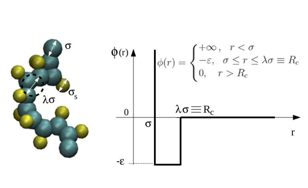
Figure 1: The square-well potential used in the models. $\sigma$ is the diameter of the beads in the backbone, $\sigma_{s}$ that of the beads representing the side chains, $-\epsilon$ is the depth of the well.

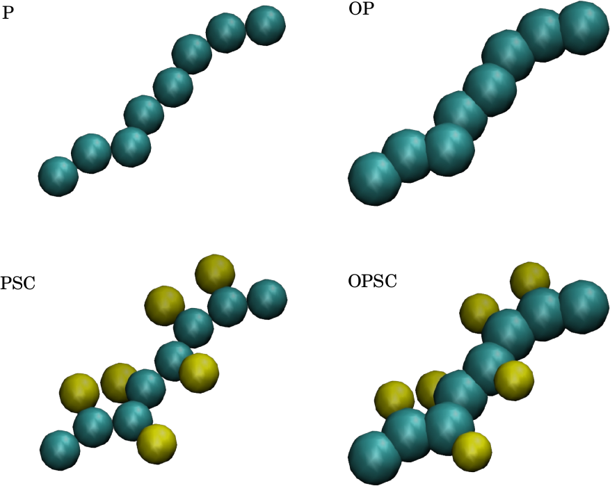
Figure 2: The four different models considered in the present study. (P) has tangent backbone beads $b/\sigma=1$ and no side chains $\sigma_{s}=0$. (OP) has no side chains but its backbone is formed by overlapping beads $b/\sigma<1$. (PSC) has side chains $\sigma_{s}>0$ but no overlap $b/\sigma=1$. (OPSC) has side chains $\sigma_{s}>0$ and overlapping beads in the backbone $b/\sigma<1$.

III Thermodynamics in the Wang-Landau approach

In the micro-canonical approach, the central role is played by the density of states (DOS) $g(E)$ that is related to the micro-canonical entropy as

$$S\left(E\right) = k_{B}\ln g\left(E\right),$$ (7)

($k_{B}$ is the Boltzmann constant) and hence to the whole thermodynamics. Canonical averages can be also computed using the partition function

$$Z\left(T\right) = \sum_{E}g\left(E\right)e^{-E/\left(k_{B}T\right)},$$ (8)

and the probability function

$$P\left(E,T\right) = \frac{1}{Z\left(T\right)}g\left(E\right)e^{-E/\left(k_{B}T\right)},$$ (9)

to find the system in a conformation with the energy $E$ and temperature $T$. Helmholtz and internal energies can then be obtained as

$$F\left(T\right)=-k_{B}T\ln Z\left(T\right)$$ (10)

$$U\left(T\right)=\left\langle E\right\rangle=\sum_{E}EP\left(E,T\right)$$ (11)

where the average $\langle\ldots\rangle$ is over the probability (9).

As we shall see, two important probes of the properties of polymers and the transitions between different ordered states are given by the heat capacity

$$C\left(T\right) = \frac{dU\left(T\right)}{dT}=\frac{\left\langle E^{2}\right\rangle-\left\langle E\right\rangle^{2}}{k_{B}T^{2}}$$ (12)

and by an averaged value of the radius of gyration Barrat03 $R_{g}^{2}=\sum_{i<j}^{N}(\mathbf{r}_{i}-\mathbf{r}_{j})^{2}/N^{2}$. This can obtained in microcanonical ensemble by constructing the distribution $P(Rg^{2},E)$ of $R_{g}$ at a given $E$ to get the micro-canonical average $\langle\ldots\rangle_{E}$ over this distribution

$$\left\langle R_{g}^{2}\right\rangle_{E} = \sum_{R_{g}}P\left(R_{g}^{2},E\right)R_{g}^{2}$$ (13)

as well as in the canonical ensemble using

$$\left\langle R_{g}^{2}(T)\right\rangle = \sum_{E}\left\langle R_{g}^{2}\right\rangle_{E}g\left(E\right)e^{-E/\left(k_{B}T\right)}.$$ (14)

It is important to remark that the derivation of thermodynamics from the $g(E)$ is quite general, and does not depend on the specific method of simulation.

IV Monte Carlo simulations

In this section, we briefly recall the main points of the Wang-Landau technique as applied to a single polymer chain, as well as the main differences with its canonical counterpart.

IV.1 Micro-canonical approach: Wang-Landau method

Following general established computational protocols Allen87 ; Frenkel02 , and Refs. Taylor09_a ; Taylor09_b for the specificities related to the polymers, we use Wang-Landau (WL) method Wang01 to sample polymer conformations according to micro-canonical distribution, by generating a sequence of chain conformations $a\to b$, and accepting new configuration $b$ with the micro-canonical acceptance probability

$$P_{acc}(a\rightarrow b)=\min{\left(1,\frac{w_{b}g(E_{a})}{w_{a}g(E_{b})}\right)},$$ (15)

where $w_{a}$ and $w_{b}$ are weight factors ensuring the microscopic reversibility of the moves.

A sequence of chain conformations is generated using a set of Monte Carlo moves, which are accepted or rejected according to Eq. 15. The set of Monte Carlo moves employed consists of local-type moves, such as single-bead crankshaft, reptation and end-point moves; as well as of non-local-type moves such as pivot, bond-bridging and back-bite moves. All moves are chosen at random and one sweep of the Wang-Landau algorithm is considered completed as soon as at least N monomer beads have been displaced.

The bond-bridging moves and back-bite types of the moves are found to be important in order to sample correctly and efficiently the low-energy states. Both of them consist of selecting one chain end (bead $1$ or $N$, old end bead in the following) and attempting to connect it to an interior bead $i$ randomly chosen among its neighbourhood within $2\sigma$ range. In the bond-bridging version of the move Taylor09_b ; Dellago14 this attempt is achieved by removal of the bead next to the chosen one in the direction of the chosen end (bead $i-1$ or $i+1$) and its re-insertion between the bead $i$ and the old-end bead via a crankshaft type of the move. The factor that in this case ensures the microscopic reversibility of the move reads $w_{b}/w_{a}=n_{a}\mathrm{\,}r_{b}/n_{b}\mathrm{\,}r_{a}$, where $n_{a}$ and $n_{b}$ are the numbers of neighbours of the old and the new chain end within the $2\sigma$ range, respectively; $r_{a}$ and $r_{b}$ are the distances between (old and new) chain ends and the $i-$th bead. In the back-bite version of the move Virnau10 the old chain end ($1$ or $N$) is attempted to be directly connected with the randomly selected bead $i$ in its neighbourhood and the correction of the acceptance probability in this case is simply $w_{b}/w_{a}=n_{a}/n_{b}$. The weight factors for other types of Monte Carlo moves are all equal to unity.

IV.2 Canonical approach: replica exchange

The parallel tempering (or replica exchange) technique Swendsen86 ; Geyer91 is a powerful method for sampling in systems with rugged energy landscape. It allows the system to rapidly equilibrate and artificially cross energy barriers at low temperatures. Furthermore, the method can be easily implemented on a parallel computer. Parallel tempering technique can be used with both Monte Carlo and Molecular Dynamics simulations, but in this study, we apply this technique specifically to Monte Carlo simulation. The method entails monitoring $M$ canonical simulations in parallel at $M$ different temperatures, $T_{i}$, $i=1,2,\ldots,M$. Each simulation corresponds to a replica, or a copy of the system in thermal equilibrium. In individual Monte Carlo simulations, new moves are accepted with standard acceptance probabilities given by the Metropolis method Metropolis . The replica exchange technique allows the swapping of replicas at different temperatures without affecting the equilibrium condition at each temperature. Specifically, given two replicas $\Gamma_{i}$ being at $T_{i}$ and $\Gamma_{j}$ being at $T_{j}$, the swap move leads to a new state, in which $\Gamma_{i}$ is at $T_{j}$ and $\Gamma_{j}$ is at $T_{i}$. The acceptance probability of such a move can be derived based on the detailed balance and is given by:

$$P_{\mathrm{swap}} = \min\left(1,\exp\left[\left(\frac{1}{k_{B}T_{i}}-\frac{1}{k_{B}T_{j}}\right)(E_{i}-E_{j})\right]\right).$$ (16)

The choice of replicas to perform an exchange can be arbitrary, but for a pair of temperatures, for which replicas are exchanged, the number of swap move trails must be large enough to ensure good statistics. The efficiency of a parallel tempering scheme depends on the number of replicas, the set of temperatures to run the simulations, how frequent the swap moves are attempted, and is still a matter of debate. It has been suggested that for the best performance, the acceptance rate of swap moves must be about 20% Rathore05 .

V Results

V.1 Model P

Before tackling more complex systems, we will test our WL and replica exchange approaches using the simple, and yet interesting, P model ($\sigma/b=1$ and $\sigma_{s}=0$) for which several studies Taylor09_a ; Taylor09_b have been previously performed and can then be contrasted with.

The aim of the calculation is the computation of the DOS $g(E)$. In the WL method, $g(E)$ is constructed iteratively, with smaller scale refinements made at each level of iteration, controlled by the flatness of energy histogram. We typically consider an iteration to reach convergence after $30$ levels of iteration, corresponding to a multiplicative factor values of $f=10^{-9}$. This choice is neither unique, nor universally accepted Seaton09 ; Zhou05 ; Belardinelli07 ; Swetnam11 , but we have checked this to be sufficient for our purposes by comparing results obtained with different values. An additional crucial step in WL algorithm hinges in the selection of ground state energy. As this must be defined at the outset, and is known to drastically affect the low-energy behavior of the system Wust08 ; Seaton09 , care must be exercised in its selection. At the present time, however, there is no universally accepted procedure for off-lattice Wang-Landau simulations. Here we will be following the procedure suggested in Refs. Taylor09_a ; Taylor09_b , that has been reported to be reliable in most cases. A preliminary run with no low-energy cutoff is carried out for a sufficient number of MC steps ($10^{9}$ in our case). This provides an estimate of the low energy cut-off, that can then be increased by $1\%$ percent and used throughout successive calculations.

In our parallel tempering scheme we consider 20 replicas and the temperatures are chosen such that they decrease geometrically $T_{i+1}=\alpha T_{i}$, where $\alpha=0.8$, starting from the highest reduced temperature $k_{B}T_{1}/\epsilon=10$, at which the polymer is well poised in the swollen phase. We allow replica exchange only between neighboring temperatures and for each replica a swap move is attempted every 50 Monte Carlo steps. Standard pivot and crank-shaft move sets Sokal are used in Monte Carlo simulations. A typical length of the simulations is $10^{9}$ steps per replica. Results from parallel tempering simulations are the equilibrium data and are convenient for analysis using the weighted histogram analysis method Ferrenberg89 . The latter allows an estimate of the density of states as well as to calculate the thermodynamic averages from simulation data at various equilibrium conditions.

We have explicitly performed both procedures for chains ranging from $N=4$ to $N=128$, as depicted in Fig. 3 where the reduced minimum energy per monomer $-E_{min}/(N\epsilon)$ is plotted against $1/N$. The results are in perfect agreement with each other and with those obtained in the extensive simulations by Taylor et al Taylor09_a ; Taylor09_b .

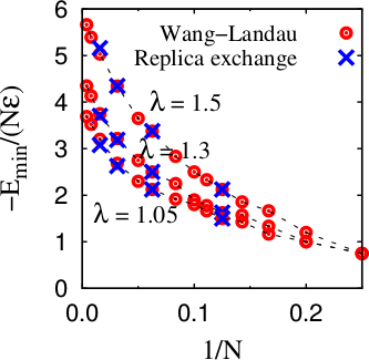
Figure 3: Plot of the reduced minimum energy per monomer $-E_{min}/(N\epsilon)$ as a function of $1/N$ for $\lambda=1.5$, using both canonical (crosses) and Wang-Landau (circles) approaches.

As an additional preliminary step, we have tested our WL code against exact analytical results valid for small $N=4$ (tetramers) and $N=5$ (pentamers) Taylor95 ; Taylor03 ; Magee08 at different values of the interaction range $\lambda$. A final test stems from a comparison with the Molecular Dynamics (MD) and canonical Monte Carlo (MC) results by Zhou and Karplus Zhou97 . In all cases, we have found complete agreement, as detailed in the supplementary information.

The successfull comparison with previous results of past literature on the P model, gave us confidence about the reliability of our computational tools. A particularly interesting results, originally derived by Taylor et al Taylor09_a ; Taylor09_b and reproduced by our calculations (see supplementary information Fig2S), hinges upon the interaction range dependence of the low temperature state of the polymer. Upon cooling from a high temperature coil state, the chain P first exhibits a transition to a collapsed globule and then to a frozen crystallyte. However, for very short-range interaction ($\lambda<1.05$), the continuous collapse transition is pre-empted by the freezing transition, and there is a direct first-order coil-crystallite transition. Interestingly, this range dependence mirrors a similar dependence destabilizing the liquid phase in favour of the solid phase in SW fluids Pagan05 .

As we will see below, we will observe something similar in the coil-helix transition of the OPSC model.

V.2 From Model P to Model OPSC

Having discussed the P model as a suitable model for polymers, we now add additional ingredients in our strive toward a model for a protein. While the P model is perfectly able to describe the correct low temperature behaviour of polymers, it cannot be used for proteins not even at the minimal level of description. There are a number of reasons for that. Previous results Taylor09_a ; Taylor09_b briefly recalled in Section V.1, unambiguously showed that a model of a chain formed by tethered spherical beads can only have a high temperature coil phase, an intermediate globular phase – provided the range of interactions to be sufficiently long – and a low temperature crystal phase. Due to its inherent isotropy, the P model cannot capture the essential ingredients for the formation of secondary structures in proteins.

One possibility to cope with this is to replace beads with disks, thus breaking the spherical symmetry. In a continuum description, this gives rise to the so-called tube (or thick polymer) model Maritan00 ; Banavar03 . This effect alone was shown to give rise to formation of helices and planar conformations Poletto08 . The tube model, however, requires a three-body potential Maritan00 ; Banavar03 , and is then very demanding from the computational viewpoint. A similar effect can be achieved by allowing partial overlapping of consecutive spherical monomers, giving rise to model OP considered here. In the OP model consecutive spheres overlap ($b/\sigma<1$) but side chains are absent ($\sigma_{s}=0$). Another ingredient that is known to play a fundamental role in the low temperatures behavior of proteins is the steric hindrance of the side chains. This can be seen, for instance, from the Ramachandran plots in real proteins showing that both alpha helices and beta sheets are constrained into well defined regions of the dihedral angles Finkelstein02 . One can then envisage the possibility of introducing additional spherical beads, attached to each backbone bead at the appropriate location and representing the van der Waals spheres of the side chains. This leads to the PSC model that is complementary to the OP model in the sense that consecutive spheres do not overlap ($b/\sigma=1$) but side chains are present ($\sigma_{s}>0$). Finally, one can consider both effects, thus obtaining the OPSC model. Note that both backbone and side chain spheres are considered aspecific, unlike in real proteins where both have their own specific character. The effect of this ingredient has been considered in the past and therefore will be neglected for simplicity in the present work, although in principle it could be accounted for without any difficulties.

V.3 Model OPSC

We now focus on the OPSC model as that of main interest for the present work. The OPSC model was already considered in Ref. Banavar09 using the replica-exchange canonical simulations, both for short ($N=16$) and long ($N=50$) chains. The necessary effort for reaching the correct ground state was considerable for the longer chain case, due to the appearance of an increasing number of metastable configurations that might hamper the correct low temperature sampling. In the present study, we will extend results obtained in Ref.Banavar09 via a Wang-Landau method that will shed new light on the OPSC model within a wider perspective. We will obtain the complete phase diagram in the temperature-interaction range plane that highlights the fundamental role of the range of interaction on the formation of the secondary structures.

In OPSC consecutive spheres overlap ($b/\sigma<1$) and side chains are present ($\sigma_{s}>0$). Here, we will use both dimensionless and dimensional units to make contacts with both general features of the P model previously discussed, and with realistic values characteristic of protein systems. As in Ref.Banavar09 , we will use $N=16,50$, $\sigma=6$Å and $\sigma_{s}=5.0$Å and $b=3.8$Å. The range of interactions here is set to $R_{c}=7.5$Å. This corresponds to $b/\sigma\approx 0.63$, $\sigma_{s}/\sigma\approx 0.83$, and $\lambda=R_{c}/\sigma\approx 1.25$ in dimensionless units. The WL calculation was performed by using different ground state energies from $E_{gs}/\epsilon=-55$ to $E_{gs}/\epsilon=-60$, and Fig. 4 reports the specific heat per monomer $C_{V}/(Nk_{B})$. In this case, the lower bound energies are simply set by the interval of values one is considering when filling the energy histograms. In practice, all energies lower than these predefined cut-off are discarded. Here $N=16$ as in Ref. Banavar09 . While the first peak at higher temperatures, associated with the coil-to-globule transition, is unaffected by the actual value of the ground state, the different behavior at low temperatures is clearly visible. When $E_{gs}/\epsilon=-55$ the low temperature second peak is absent, indicating that the ground state is the double helix structure. Note that the double helix is stabilized by consecutive non-local contacts, in the same way as protein’s $\beta$-sheets, but lacks the planar symmetry of the latter. As the energy decreases toward the correct ground state $E_{gs}/\epsilon=-60$, a second low temperatures peak emerges indicating an additional structural transition to a helical state, that is then the ground state of the system under these conditions. Note that the results for $E_{gs}/\epsilon=-60$ are in full agreement with those obtained in Fig.3a of Ref.Banavar09 via replica-exchange canonical simulations.

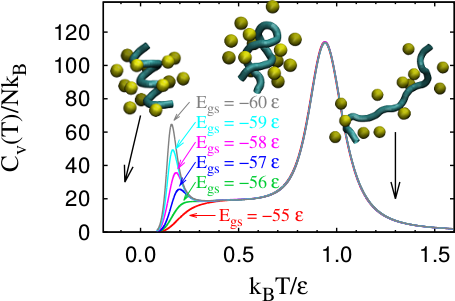
Figure 4: Specific heat per monomer $C_{V}/(Nk_{B})$ as a function of the reduced temperature $k_{B}T/\epsilon$ in the case $N=16$ with different ground state energies $-60\leq E_{gs}/\epsilon\leq-55$ These results for $E_{gs}/\epsilon=-60$ are compatible with Fig.3a of Ref.Banavar09 . The insets include snapshots of rapresentative configurations (helix on the left, double helix in the middle and the coil on the right). Here and below, a tube representation of the backbone is employed for a better visual reproduction.

Even when the actual low energy limit is properly accounted for, the corresponding ground state is strongly dependent upon the chosen range of the interactions $R_{c}$. This is not surprising on physical grounds. As $R_{c}/\sigma\approx 1$, the range of attraction is essent

ers, and the chain will have the tendency to form a coil configuration at high temperatures and a suitable secondary structure maximizing the number of favorable contacts at low temperatures. In the opposite limit $R_{c}/\sigma\gg 1$, each monomer can interact with essentially any other monomer in the chain, and at low temperature will tend to form a globular structure that displays the lowest possible energy. On the basis of results given in Fig. 4 for $N=16$, one could reasonably expect a formation of a stable helix for some intermediate value of the $R_{c}/\sigma$ ratio. This is confirmed in Fig. 5, where we report the specific heat per monomer $C_{V}/(Nk_{B})$ as a function of the reduced temperature $k_{B}T/\epsilon$ in the case $N=16$ (top panel) and $N=50$ (bottom panel), at different ranges of interactions $R_{c}$. In the former case ($N=16$) a single well-developed peak is clearly visible for $R_{c}=6.5$Å, corresponding to the coil-helix transition. As $R_{c}$ increases, this single peak gradually evolves first into two, around $R_{c}\approx 7.5$Å, and eventually into three at $R_{c}\approx 9.0$Å, accounting for an intermediate double helix configuration at $k_{B}T/\epsilon\approx 0.8$, and for a globular configuration at the lowest $k_{B}T/\epsilon$. The $N=16$ result is particularly useful because it allows the presence also of larger values of $R_{c}$ that typically require long computational time.

We note that these results extend those presented in Fig.S2(a) in the supplementary information of Ref.Banavar09 obtained by replica-exchange canonical simulations. In all cases the ground state energies were found identical (dependent on the choice of $R_{c}$).

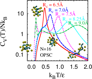
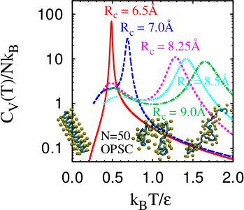
Figure 5: (Top) Specific heat per monomer $C_{V}/(Nk_{B})$ as a function of the reduced temperature $k_{B}T/\epsilon$ in the case $N=16$ with different interaction ranges $R_{c}$. (Bottom) Same as above in the case $N=50$. In this case, the results for $R_{c}=6.5$Å are compatible with Fig.S2(a)in the supplementary information of Ref.Banavar09 .

The case $N=50$ allows for a better statistics at the expense of an increased computational effort, see Fig. 5 (bottom panel). A striking feature of Fig. 5 is again the presence of a single strong peak indicating the ground state of the system corresponding to a helical organization, as illustrated in the insert snapshot, along with a secondary peak at slightly higher temperatures. The second peak increases, and in fact becomes the dominant one, upon increasing the interaction range $R_{c}$, indicating the progressive stabilization of the double helix phase found at intermediate temperatures. This is in line with previous results for $N=16$ with the proviso that the globular phase is missing here due to the fact that the computational effort becomes prohibitively large for $R_{c}\gg 9$ Å, a region where this phase is expected. Compatible results (not shown) can be obtained also by considering the gyration radius, in analogy to what done in the P model case.

Guided by the above findings, we can now draw the phase diagram in the temperature $k_{B}T/\epsilon$ - interaction range $R_{c}$ plane. This complements those already obtained in Ref.Banavar09 in the $\sigma_{s}-\sigma$ plane and is reported in Figure 6 in the case $N=16$ (top panel) and $N=50$ (bottom panel). Here $\sigma=6$Å and $\sigma_{s}=5$ Å.

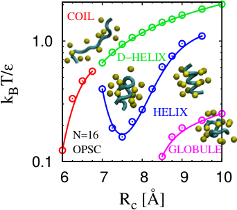
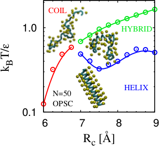
Figure 6: Phase diagram of the OPSC model in the temperature-interaction range plane.(Top) $N=16$ case. (Bottom) $N=50$ case.

Several interesting features are apparent. Starting from a coil high temperature configuration, one finds a direct transition to a helix conformation upon cooling for sufficiently short interaction ranges ($R_{c}\leq 7$ Å). Above this value, there is first a transition to a double helix structure followed by a successive transition to helix structure. The two transitions are expected to merge at large interaction range, where the low temperature ground state is presumed to be a globule, irrespective of $R_{c}$. Note that the characteristic dual helix structure appearing in the $N=16$ case evolves into a more complex structure where the internal helical shape is bracketed by double-helicies at chain endings, connected via flexible turns. We dubbed this hybrid configurations in the lower panel of Figure 6.

V.4 Model OP

We now backtrack to investigate the effect of removing one-by-one single ingredients in the resulting phase diagram.

In the OP model, consecutive beads overlap, as in the OPSC model, but here the side chains are missing ($\sigma_{s}=0$), so that the steric hindrance of the side chain beads is also absent. On the other hand, partial interpenetration of consecutive beads breaks the spherical symmetry of the P model, along the backbone direction. Effectively, this provides a restriction on the number of possible local conformations that the chain can achieve as its effective shape becomes more cylindrical. A similar effect can be obtained in the tube model by enforcing a finite thickness of the chain but it requires a three-body potential Maritan00 . In the $N=16$ case, for high and low temperatures the coil and globule conformations are respectively observed, with intermediate temperature phases typically as the double helical conformation at low $R_{c}$ and a helicoidal conformation at larger $R_{c}$. This agrees with findings from the tube model, in spite of the different driving forces in the two systems Poletto08 . These results also complement those obtained via replica exchange simulations by Magee and collaborators Magee07 ; Magee08 who observed helix formation in the OP model for sufficiently high interpenetration with $N=20$ but did not compute the phase diagram, as done here.

As the length of the polymer increases, we find these intermediate double helical and helicoidal configurations to become less and less stable, so that in the case of $N=50$ only a stable coil and globular configurations, with some intermediate planar-like structures, are observed. In Figure 7, we display the obtained phase diagram in the case $N=50$. Interestingly, below $R_{c}\approx 6$ Å, we expect a direct coil-globule transition.

A final remark is here in order. While it is intuitive that the OP model shares some similarities with the tube model discussed in Ref. Maritan00 ; Poletto08 , since both lead to a breaking of the spherical symmetry with the appearance of a privileged axis along the chain backbone, we believe that some of the specificities of the three-body potential involved in the tube model cannot be represented by a two-body potential as discussed here.

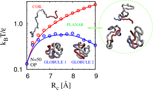
Figure 7: Phase diagram of the OP model in the temperature-interaction range plane in the $N=50$ case.

V.5 Model PSC

The OPSC model reduces to the PSC model in the absence of overlapping ($b/\sigma=1$). This was already partially considered in Ref.Banavar09 , where again a phase diagram in the $\sigma_{s}-\sigma$ plane was obtained. Our resulting phase diagram is displayed in Fig.8. When contrasted with the corresponding OPSC counterpart of Fig.6(bottom), we note a significant shrinking of the intermediate phase, as well as a reduced shape stability of the helical phase. All in all, our interpretation of these findings is that the interpenetrability of the backbone beads and the presence of the side chain beads are both crucial concurring ingredients to the observation of secondary structures, a combination of the two providing an optimal condition to their stability.

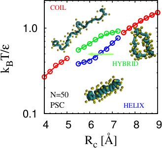
Figure 8: Phase diagram of the PSC model in the reduced temperature $k_{B}T/\epsilon$ vs interaction range $R_{c}$ plane for $N=50$. Here $\sigma=b=3.8$Å and $\sigma_{s}=5$ Å.

VI Correlation function and the Fisher–Widom line

The Landau-Peierls theorem Landau80 ; Thouless69 forbids the presence of a thermodynamic phase transition in a strictly one-dimensional system with only short range interactions, and a similar result holds true for liquid systems VanHove50 .

In fluid systems and in the presence of competing attractive/repulsive interactions, such as those occurring here, a Fisher–Widom (FW) line (not to be confused with the Widom line Franzese07 ) is separating two different regimes in the radial distribution function Fisher69 , characterized by an oscillatory (when repulsions are dominating) and an exponentially decaying (when attractions are dominating) behavior. The rationale behind the FW line is that on approaching the critical points where attractions become more and more effective, the behavior of correlation functions must switch from oscillatory (characteristic of repulsive interactions) to exponential with a well defined correlation length. The FW line was also observed in one-dimensional fluid of penetrable spheres Fantoni09 ; Fantoni10 , where Landau-Peierls theorem is no longer valid. In practice, the FW line is associated with an abrupt discontinuity in the structural behaviour of the system (as signalled by the correlation function) that is not, however, related to any real discontinuity in the thermodynamical behaviour.

As shown below, a similar feature occurs in the present framework where the abrupt change in a correlation function is indicative of a structural transition, preceeding (i.e. occurring at slightly higher temperatures) the actual thermodynamical transitions, that will then be interpreted as the countepart of the FW line.

Consider the tangent-tangent correlation function $G_{l}$ defined in Eq.(5) as a function of the sequence separation (distance of the beads along the chain) $s$. In the coil state, the conformation of the chain is random and hence there is no correlation between the orientations of consecutive backbone beads. As a result, the tangent-tangent correlation is an exponentially decaying function of the sequence separation. In the helix state, however, the tangent-tangent correlation is an oscillating function of the sequence, with periodicity of about 4 units. The transition between the two regimes is an abrupt one, and occurs at temperatures slightly higher than those associated with the actual coil-to-helix transformation. Figure 9 confirms this expectation. Here the tangent-tangent correlation is plotted as a function of the sequence separation at four different reduced temperatures, $k_{B}T/\epsilon=0.6$ above the FW line, $k_{B}T/\epsilon=0.5$ at the FW line, $k_{B}T/\epsilon=0.485$ at the coil-helix transition, and $k_{B}T/\epsilon=0.47$ below it. The transition from an exponential to an oscillating behavior upon cooling below the FW line is thus evident. Note that this transition can be experimentally probed by e.g. circular dichroism, and some straightforward procedures have been devised to interpret the results of these measurements in terms of simple spin models Badasyan10 ; Badasyan12 . Similar transitions also occur for the normal-normal and binormal-binormal correlations as shown in the supplementary information (see Figures 3Sa, 3Sb and 3Sc).

Our findings agree with those by Banavar et al Banavar09 obtained via the replica-exchange method, where the onset of oscillations in the tangent-tangent correlation as a function of the sequence separation, was taken as an indicator of the incipient coil-helix transition.

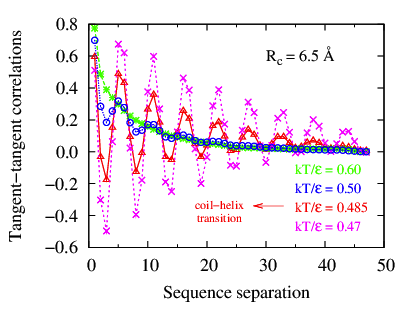
Figure 9: Plot of the tangent-tangent correlation functions as a function of the sequence separation at four different reduced temperatures $k_{B}T/\epsilon$: above the Fisher-Widom line ($k_{B}T/\epsilon=0.6$), at the Fisher-Widom line ($k_{B}T/\epsilon=0.5)$, at the coil-helix transition ($k_{B}T/\epsilon=0.485)$, and below it ($k_{B}T/\epsilon=0.47)$.

VII Conclusions

In this paper we have studied the equilibrium statistics of a homopolymer formed by a sequence of tangent identical monomers represented by impenetrable hard spheres. A tethering potential keeps the consecutive backbone beads linked, whereas non-consecutive ones interact via a square-well potential, that then drives the collapse of the chain at sufficiently low temperatures. Three different variants of the above P model were considered as a gradual step toward a more realistic model for proteins. By allowing consecutive backbone spheres to interpenetrate, one breaks the rotational symmetry of the P model, thus opening up the possibility of having additional intermediate transitions. This model, dubbed the OP model, is similar in spirit to the tube model Maritan00 ; Banavar03 , where the symmetry breaking was enforced by replacing spherical with disk-like beads. Another variant, denoted as PSC model, keeps the backbone beads tangent, but allows the presence of additional side-chain beads located at appropriate position of the side chain center in real proteins. The interest in this variant is triggered by some some studies suggesting the importance of the role of side chains in the formation of secondary structures Yasuda10 . The last variant, the OPSC model, combines all of the above effects.

As a preliminary validation of our approach, we first reproduced some of the Wang-Landau results obtained by Taylor et al Taylor09_a ; Taylor09_b for model P, with long chains (with up to $N=256$ monomers) that we also re-obtained via replica-exchange canonical approach. This comparison allows us to be confident in the reliability of our computational scheme.

Having done that, we have then used the same Wang-Landau method to tackle OP, PSC, and OPSC models. The latter can be regarded as a minimal model for the formation of secondary structures in proteins and was studied by replica-exchange techniques in Ref. Banavar09 . In particular, we were able to underpin the fundamental role played by the interaction range in selecting the secondary structure. For very short range square-well attractions, the lowest energy is achieved by a double helix, in agreement with our intuition and with previous findings on the tube model Poletto08 . At intermediate interaction range, the lowest energy is associated with the formation of a well-defined helical structure, whereas at interaction ranges much longer of the bead sizes, the ground state is a globule, as expected in view of its mean-field like character. The possibility of tuning a single coil-to-globule or a double coil-to-helix and helix-to-globule transition, can be regarded as the OPSC model counterpart of the results found in the P model by Taylor et al Taylor09_a ; Taylor09_b , where the double transition coil-to-globule and globule-to-crystal transitions found at moderate attractive range, are replaced by a direct coil-to-crystal transition below a critical interaction range, in close analogy with what is found in square-well fluids, where a double gas-liquid and liquid-solid transitions is preempted by a direct gas-solid transition below a critical range of interactions Pagan05 . Note, however, that this parallelism limits to an analogy as the coil-helix transition is a structural rather than a thermodynamical transition.

In addition to to the OPSC model, we have also studied the simpler OP model, where side chains are absent, and the PSC model, where there is no overlap between consecutive spheres. We found that both models display a phase transition similar to the full OPSC model but with a larger degree of metastability.

Finally, we have also discussed the transition in the behavior of the tangent-tangent correlation functions, as well as the the normal-normal and the binormal-binormal correlation functions, as a function of the temperature. We found that the exponental behaviour in the sequence separation characteristic of the coil configuration at high temperatures, is replaced by an oscillatory behaviour at lower temperatures, indicating a helical organization, and this occurs at temperatures higher than the actual coil-helix thermodynamic transition. We proposed this line to be regarded as the analogue of the Fisher-Widom line found in fluid systems, in such this structural transition precedes the actual thermodynamical transition associated with the discontinuity in the thermodynamical variables.

The formation of secondary structures is an important intermediate step for the general process of the folding of a protein. Our results are consistent with previous studies Maritan00 ; Banavar03 suggesting that the introduction of a cylindrical (as opposed to spherical) symmetry is in fact sufficient to remove the characteristic glassy structure of the low energy state in polymers, and highlights the presence of side chains as a further stability factor. The rigidity of the chain, mostly ascribed to the presence of intrachain hydrogen bonds, is known to be another important ingredient for protein folding that could further introduced in our analysis as a further step toward a more realistic model for a protein. Work along these lines is currently underway and will be reported in a future study.

Appendix A Phase diagrams of P model

In Figure 10 we report results obtained from Wang-Landau method applied to model P that are then used to draw the phase diagram (see Figure 11). These include both the specific heat per monomer $C_{v}(T)/(Nk_{B})$ and the reduced mean-square radius of gyration $\langle R^{2}(T)\rangle/N\sigma^{2}$ as a function of the reduced temperature $k_{b}T/\epsilon$.

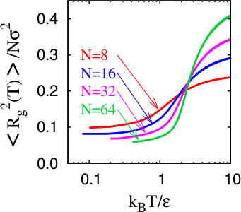
Figure 10: (Top) The specific heat per monomer $C_{v}(T)/(Nk_{B})$ as a function of the reduced temperature $k_{b}T/\epsilon$ for the P model with $N=8,16,32,64$. (Bottom) The reduced mean-square radius of gyration $\langle R^{2}(T)\rangle/N\sigma^{2}$ as a function of the reduced temperature $k_{b}T/\epsilon$ under the same canditions.

In Figure 11 the phase diagram of the P model in the reduced temperature $k_{B}T/\epsilon$ vs interaction range $R_{c}$ plane is depicted for $N=50$. Upon cooling from a coil configuration, one finds first a transition to a globule, and then a transition to a crystal. The two transitions merge below $R_{c}\approx 6$ Åto become a direct coil-crystal transition in agreement with the results by Taylor et al. At larger interaction ranges, the crystal structure becomes less definite more similar to a spherical globule as one could expect on a physical ground.

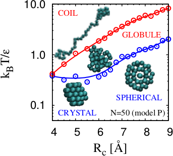
Figure 11: Phase diagram of the P model in the reduced temperature $k_{B}T/\epsilon$ vs interaction range $R_{c}$ plane for $N=50$.

Appendix B Temperature dependence of the correlation functions for the OPSC model

The three correlation functions (tangent-tangent, normal-normal, and binormal-binormal) of the OPSC model are plotted as a function of the sequence separation and of the reduced temperature $k_{B}T/\epsilon$ in Fig. 12. The transition from exponential to oscillating behavior upon cooling below a critical temperature line is evident in all three cases.

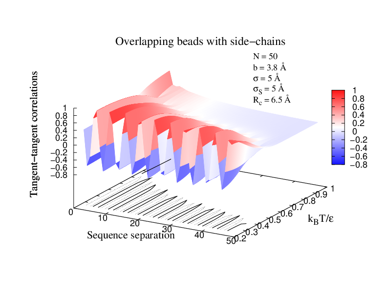
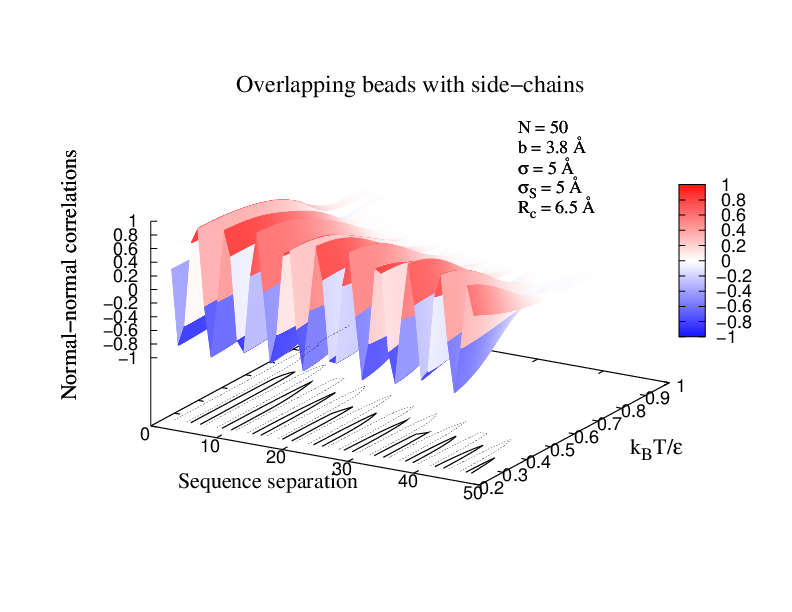
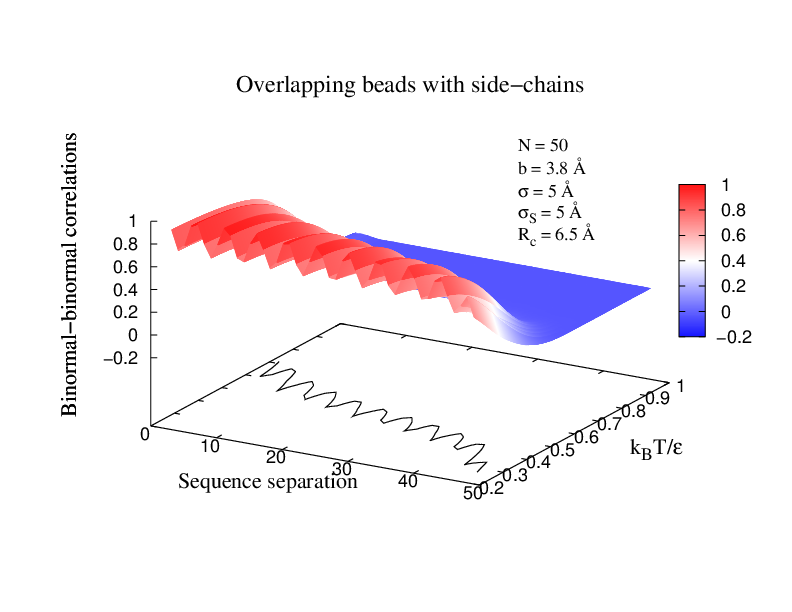
Figure 12: Three dimensional plot of the tangent-tangent, normal-normal, and binormal-binormal correlation functions as a function of the sequence separation and the reduced temperature $k_{B}T/\epsilon$.

Table 1: Comparison between the ground state energies obtained from the microcanonical Wang-Landau and the canonical replica exchange.

$\lambda=1.05$	$N$	$-E_{\text{gs}}^{\text{WL}}$	$-E_{\text{gs}}^{\text{RE}}$
	$3$	$1$	$-$
	$4$	$3$	$-$
	$5$	$5$	$-$
	$6$	$7$	$-$
	$7$	$10$	$-$
	$8$	$12$	$12$
	$9$	$15$	$-$
	$10$	$18$	$-$
	$12$	$23$	$-$
	$16$	$34$	$34$
	$20$	$46$	$-$
	$32$	$86$	$84$
	$64$	$205$	$197$
	$128$	$451$	$-$
	$256$	$945$	$-$
$\lambda=1.3$	$N$	$-E_{\text{gs}}^{\text{WL}}$	$-E_{\text{gs}}^{\text{RE}}$
	$3$	$1$	$-$
	$4$	$3$	$-$
	$5$	$5$	$-$
	$6$	$8$	$-$
	$7$	$11$	$-$
	$8$	$13$	$13$
	$9$	$16$	$-$
	$10$	$19$	$-$
	$12$	$27$	$-$
	$16$	$40$	$40$
	$20$	$55$	$-$
	$32$	$103$	$102$
	$64$	$240$	$237$
	$128$	$529$	$-$
	$256$	$1113$	$-$
$\lambda=1.5$	$N$	$-E_{\text{gs}}^{\text{WL}}$	$-E_{\text{gs}}^{\text{RE}}$
	$3$	$1$	$-$
	$4$	$3$	$-$
	$5$	$6$	$-$
	$6$	$10$	$-$
	$7$	$13$	$-$
	$8$	$17$	$17$
	$9$	$21$	$-$
	$10$	$25$	$-$
	$12$	$34$	$-$
	$16$	$54$	$54$
	$20$	$73$	$-$
	$32$	$139$	$139$
	$64$	$322$	$330$
	$128$	$690$	$-$
	$256$	$1450$	$-$

- (1) J. P. Hansen and I. R. McDonald, Theory of Simple Liquids (Academic, New York, 1986).
- (2) B. J. Alder and T. E. Wainwright, J. Chem. Phys. 31, 459 (1959).
- (3) J. A. Barker and D. Henderson, Rev. Mod. Phys. 48, 587 (1976).
- (4) M. H. J. Hagen and D. Frenkel, J. Chem. Phys. 101, 4093 (1994).
- (5) D. L. Pagan and J. D. Gunton, J. Chem. Phys. 122, 184515 (2005).
- (6) H. Liu, S. Garde and S. Kumar, J. Chem. Phys. 123, 174505 (2005).
- (7) C. G. Gray and K. E. Gubbins, Theory of Molecular Fluids, Vol. 1: Fundamentals (Clarendon, Oxford, 1984).
- (8) J. Lyklema, Fundamentals of Interface and Colloid Science, Vol. I: Fundamentals (Academic, London, 1991).
- (9) Y. Zhou, M. Karplus, J. M. Wichert and C. K. Hall, J. Chem. Phys. 107, 24 (1997).
- (10) M. P. Taylor, Mol. Phys. 86, 73 (1995).
- (11) M. P. Taylor, J. Chem. Phys. 118, 883 (2003).
- (12) M. P. Taylor, W. Paul and K. Binder, J. Chem. Phys. 131, 114907 (2009).
- (13) M. P. Taylor, W. Paul and K. Binder, Phys. Rev. E 79, 050801(R) (2009).
- (14) A. Grosberg and A. Khokhlov, Statistical Physics of Macromolecules (AIP, New York, 1994).
- (15) K. Yue, and K. A. Dill, Proc. Natl. Acad. Sci. U.S.A. 89, 4163 (1992).
- (16) D. T. Seaton, T. Wüst and D. P. Landau, Comp. Phys. Comm. 180 587 (2009).
- (17) T. Wüst, Y. W. Li and D. P. Landau, J. Stat. Phys. 144 638 (2011).
- (18) T. Wüst and D. P. Landau, Comp. Phys. Comm. 179 124 (2008).
- (19) I. Coluzza, PLOS One 6 e20853 (2011).
- (20) J. R. Banavar, M. Cieplak, T. X. Hoang, and A. Maritan, Proc. Natl. Acad. Sci. U.S.A. 106, 6900 (2009).
- (21) J. R. Banavar and A. Maritan, Rev. Mod. Phys. 75, 23 (2003).
- (22) A. Maritan, C. Micheletti, A. Trovato and J. R. Banavar, Nature 406, 287 (2000).
- (23) B. Park and M. Levitt, J. Mol. Biol. 258, 367 (1996).
- (24) J. R. Banavar, M. Cieplak, A. Flammini, T. X. Hoang, R. D. Kamien, T. Lezon, D. Marenduzzo, A. Maritan, F. Seno, Y. Snir and A. Trovato, Phys. Rev. E 73, 031921 (2006).
- (25) A. V. Finkelstein and O. B. Ptitsyn Protein Physics (Academic Press 2002).
- (26) H. Taketomi, Y. Ueda and N. Go, Int. J. Pept. Protein Res. 7, 445 (1975).
- (27) C. Clementi, H. Nymeyer, and J. N. Onuchic, J. Mol. Biol. 298 937 (2000).
- (28) N. Koga and S. Takada, J. Mol. Biol. 313 171 (2000).
- (29) A. Badasyan, Z. Liu and H. S. Chan, J. Mol. Biol. 384 512 (2008).
- (30) M. P. Allen and D. J. Tildesley, Computer Simulations of Liquids (Clarendon, Oxford 1987).
- (31) F. Wang and D. P. Landau, Phys. Rev. Lett. 86 2050 (2001).
- (32) B. Smith and D. Frenkel, Understanding Molecular Simulation: From Algorithms to Applications (Academic, San Diego, 2002).
- (33) H.S.M. Coexter Introduction to Geometry (Wiley 1989)
- (34) C. Poletto, A. Giacometti, A. Trovato, J. R. Banavar, and A. Maritan, Phys. Rev. E 77, 061804 (2008).
- (35) R. Kamien, Rev. Mod. Phys. 74, 953 (2002).
- (36) S. M. Bhattacharjee, A. Giacometti, and A. Maritan, J. Phys.: Condens. Matter, 25, 503101-503132 (2013).
- (37) J. L. Barrat, and J. P. Hansen, Basic Concepts for Simple and Complex Liquids (Cambridge University Press, Cambridge) (2003).
- (38) C. Leitold and C. Dellago, J. Chem. Phys. 141, 134901 (2014).
- (39) D. Reith and P. Virnau, Comp. Phys. Comm. 181, 800 (2010).
- (40) R. H. Swendsen and J.-S. Wang, Phys. Rev. Lett. 57, 2607 (1986).
- (41) C. J. Geyer, In Computing Science and Statistics: Proceedings of the 23rd Symposium on the Interface, p. 156, New York, 1991. American Statistical Association.
- (42) N. Metropolis, A. W. Rosenbluth, M. N. Rosenbluth, A. H. Teller and E. Teller, J. Chem. Phys. 21, 1087 (1953).
- (43) N. Rathore, M. Chopra, and J. J. de Pablo, J. Chem. Phys. 122 122, 024111 (2005).
- (44) A. D. Sokal, Nucl. Phys. B 47, 172 (1996).
- (45) A. M. Ferrenberg, & R. H. Swendsen, Optimized Monte Carlo data analysis, Phys. Rev. Lett. 63, 1195-1198 (1989).
- (46) C. Zhou and R.N. Bhatt, Phys. Rev. E 72 025701(R) (2005).
- (47) A.D. Swetnam, M.P. Allen, J. Comp. Chem. 32 816 (2011).
- (48) R.E. Belardinelli and V.D. Pereyra, Phys. Rev. E 75 046701 (2007).
- (49) J.E. Magee, L. Lue, and R.A. Curtis, Phys. Rev. E 78 031803 (2008).
- (50) J. E. Magee, Z. Song, R.A.Curtis, and L. Lue, J. Chem. Phys. 126, 144911 (2007)
- (51) Landau L. D. and Lifshitz E. M., Statistical physics, Vol. 5 of Course of Theoretical Physics (Butterworth-Heinemann) 1980.
- (52) Thouless D. J., Phys. Rev., 187, 732 (1969).
- (53) L. Van Hove, Physica (Amsterdam) 16, 137 (1950).
- (54) G. Franzese, H. E. Stanley, J. Phys.: Condens. Matter 19, 205126 (2007).
- (55) M.E. Fisher and B. Widom, J. Chem. Phys. 50, 3756 (1969)
- (56) R. Fantoni, A. Giacometti, Al. Malijewski, and A. Santos, J. Chem. Phys. 133, 024101 (2010).
- (57) R. Fantoni, A. Giacometti, Al. Malijevský, and A. Santos, J. Chem. Phys. 131, 124106 (2009).
- (58) A. Badasyan, S. Tonoyan, A. Giacometti, R. Podgornik, and V. A. Parsegian, Phys. Rev. Lett. 109, 068101 (2012).
- (59) A. Badasyan, A. Giacometti, Y. Sh. Mamasakhlisov, V.F. Morozov and A. S. Benight, Phys. Rev. E, 81, 021921 (2010).
- (60) S. Yasuda, T. Yoshidome, H. Oshima, R. Kodama, Y. Harano, and M. Kinoshita, J. Chem. Phys. 132, 065105 (2010).