Computational Soundness Results for
Stateful Applied $\pi$ Calculus

Abstract

In recent years, many researches have been done to establish symbolic models of stateful protocols. Two works among them, the SAPIC tool and StatVerif tool, provide a high-level specification language and an automated analysis. Their language, the stateful applied $\pi$ calculus, is extended from the applied $\pi$ calculus by defining explicit state constructs. Symbolic abstractions of cryptography used in it make the analysis amenable to automation. However, this might overlook the attacks based on the algebraic properties of the cryptographic algorithms. In our paper, we establish the computational soundness results for stateful applied $\pi$ calculus used in SAPIC tool and StatVerif tool.

In our approach, we build our results on the CoSP framework. For SAPIC, we embed the non-monotonic protocol states into the CoSP protocols, and prove that the resulting CoSP protocols are efficient. Through the embedding, we provide the computational soundness result for SAPIC (by Theorem 1). For StatVerif, we encode the StatVerif process into a subset of SAPIC process, and obtain the computational soundness result for StatVerif (by Theorem 2). Our encoding shows the differences between the semantics of the two languages. Our work inherits the modularity of CoSP, which allows for easily extending the proofs to specific cryptographic primitives. Thus we establish a computationally sound automated verification result for the input languages of SAPIC and StatVerif that use public-key encryption and signatures (by Theorem 3).

1 Introduction

Manual proofs of security protocols that rely on cryptographic functions are complex and known to be error-prone. The complexity that arises from their distributed nature motivates the researches on automation of proofs. In recent years, many efficient verification tools ([1, 2, 3]) have been developed to prove logical properties of protocol behaviors. To eliminate the inherent complexity of the cryptographic operations in formal analysis, these verification tools abstract the cryptographic functions as idealized symbolic terms that obey simple cancelation rules, i.e., the so-called Dolev-Yao models ([4, 5]). Unfortunately, these idealizations also abstract away from the algebraic properties a cryptographic algorithm may exhibit. Therefore a symbolic formal analysis may omit attacks based on these properties. In other words, symbolic security does not immediately imply computational security. In order to remove this limitation, the concept of Computational Soundness (CS) is introduced in [6]. From the start, a large number of CS results over the past decade were made to show that many of the Dolev-Yao models are sound with respect to actual cryptographic realizations and security definitions (see, e.g., [7, 8, 9, 10, 11, 12, 13, 14, 15]).

More recently, formal analysis methods have been applied to stateful protocols, i.e., protocols which require non-monotonic global state that can affect and be changed by protocol runs. Stateful protocols can be used to model hardware devices that have some internal memory and security APIs, such as the RSA PKCS#11, IBM’s CCA, or the trusted platform module. There are many formal methods that have been used to establish symbolic model of stateful protocols ([16, 17, 18, 19, 20, 21, 22]). Two works among them, the SAPIC tool [20] and StatVerif tool [21], can provide an automated analysis of stateful protocols. Their language, the stateful applied $\pi$ calculus, is extended from the applied $\pi$ calculus [23] by defining constructs for explicitly manipulating global state. One advantage of the stateful applied $\pi$ calculus is that it provides a high-level specification language to model stateful protocols. Its syntax and semantics inherited from the applied $\pi$ calculus can arguably ease protocol modeling. Another advantage is that the formal verification can be performed automatically by these tools.

However, no CS works have been done for the stateful applied $\pi$ calculus. Although there are many for the original applied $\pi$ calculus, e.g., see [11, 15, 24]. Our purpose is to establish the CS results for the input languages of the two verification tools SAPIC and StatVerif. With our results, we can transform their symbolically automated verification results of stateful protocols (with some restrictions) to the computationally sound one with respect to actual cryptographic realizations and security definitions. We want to establish the CS results directly for the input languages of SAPIC and StatVerif. To achieve this, we choose to embed them into the CoSP work [11], a general framework for conceptually modular CS proofs. Since the stateful applied $\pi$ calculus used in SAPIC and StatVerif are slightly different, in the following we call the former SAPIC calculus and the latter StatVerif calculus.

Our work. We present two CS results respectively for the stateful applied $\pi$ calculus used in SAPIC tool and StatVerif tool. In our approach, we first provide the method to embed SAPIC calculus into the CoSP framework. Note that the CoSP framework does not provide explicit state manipulation. We need to embed the complex state constructs of stateful applied $\pi$ calculus into the CoSP protocols and make sure that the resulting CoSP protocol is efficient. By the embedding, we prove that the CS result of applied $\pi$ calculus implies that of SAPIC calculus (by Theorem 1). For StatVerif, we provide an encoding of StatVerif processes into a subset of SAPIC processes and build the CS result of StatVerif calculus (by Theorem 2). Our encoding shows the differences between the semantics of these two languages. Finally, we establish a computationally sound automated verification result for the input languages of SAPIC and StatVerif that use public-key encryption and signatures (by Theorem 3).

For SAPIC, we use the calculus proposed by [20] as the SAPIC calculus. It extends the applied $\pi$ calculus with two kinds of state: the functional state and the multiset state. We set two restrictions respectively for the pattern matching in the input constructs and for the multiset state constructs. They are necessary for the computational execution model. We embed the SAPIC calculus into the CoSP framework. The two kinds of state are encoded into the CoSP protocol state (as part of the CoSP node identifiers). We have met two challenges in the embedding. First is for the functional state. If we encode them directly as $\pi$-terms, the resulting CoSP protocol is not efficient. Thus we transform them into the CoSP terms which are treated as black boxes by CoSP protocols. The second problem is for the encoding of multiset state. By our restriction of multiset state constructs, we can transform the arguments of facts into CoSP terms and limit the growth of the size of multiset state. We also provide an efficient CoSP sub-protocol to implement the pattern matching in the multiset state constructs. At last, we prove that our embedding is an efficient and safe approximation of the SAPIC calculus, and build the CS result of SAPIC calculus upon that of applied $\pi$ calculus (by Theorem 1).

For StatVerif, we use the calculus proposed by [21] as the StatVerif calculus. It has minor differences to SAPIC calculus. We first provide an encoding of the StatVerif processes into a subset of SAPIC processes. Then we prove that by using SAPIC trace properties our encoding is able to capture secrecy of stateful protocols. With the CS result of SAPIC, we can directly obtain the CS result of StatVerif calculus (by Theorem 2). Our encoding shows the differences between the semantics of state constructs in these two calculi.

Note that our contribution is a soundness result for the execution models that can manipulate state, rather than a soundness result for any new cryptographic primitives. The advantage of our CS result is its extensibility, since we build it on the CoSP framework and involve no new cryptographic arguments. It is easy to extend our proofs to additional cryptographic abstractions phrased in CoSP framework. Any computationally sound implementations for applied $\pi$ calculus that have been proved in CoSP framework can be applied to our work. To explain its extendibility, we establish a computationally sound automated verification result for the input languages of SAPIC and StatVerif that use public-key encryption and signatures (by Theorem 3). We have verified the classic left-or-right protocol presented in [21] by using these tools in a computationally sound way to show the usefulness of our result.

The paper is organized as follows. In Section 2 we give a brief introduction to the CoSP framework and the embedding of applied $\pi$ calculus. In Section 3 and Section 4 we respectively show the CS results of stateful applied $\pi$ calculus in SAPIC and StatVerif work. Section 5 contains a case study of the CS result of public-key encryption and signatures. We conclude in Section 6.

2 Preliminaries

2.1 CoSP Framework

Our CS results are formulated within CoSP [11], a framework for conceptually modular CS proofs. It decouples the treatment of cryptographic primitives from the treatment of calculi. The results in [15] and [24] have shown that CoSP framework is capable of handling CS with respect to trace properties and uniformity for ProVerif. Several calculi such as the applied $\pi$ calculus and RCF can be embedded into CoSP ([11, 25]) and combined with CS results for cryptographic primitives. In this subsection, we will give a brief introduction to the CoSP framework.

CoSP provides a general symbolic model for abstracting cryptographic primitives. It contains some central concepts such as constructors, destructors, and deduction relations.

Definition 1 (Symbolic Model). A symbolic model $\textbf{M}=(\textbf{C},\textbf{N},\textbf{T},\textbf{D},\vdash)$ consists of a set of constructors C, a set of nonces N, a message type T over C and N with $\textbf{N}\subseteq\textbf{T}$, a set of destructors D over T, and a deduction relation $\vdash$ over T. A constructor $C/n\in\textbf{C}$ is a symbol with (possible zero) arity. A nonce $N\in\textbf{N}$ is a symbol with zero arity. A message type T is a set of terms over constructors and nonces. A destructor $D/n\in\textbf{D}$ of arity $n$ over a message type T is a partial map $\textbf{T}^{n}\rightarrow\textbf{T}$. If $D$ is undefined on a list of message $\underline{t}=(t_{1},\cdots,t_{n})$, then $D(\underline{t})=\bot$.

To unify notation of constructor or destructor $F/n\in\textbf{C}\cup\textbf{D}$ and nonce $F\in\textbf{N}$, we define the partial function $eval_{F}:\textbf{T}^{n}\rightarrow\textbf{T}$, where $n=0$ for the nonce, as follows: If $F$ is a constructor, $eval_{F}(\underline{t}):=F(\underline{t})$ if $F(\underline{t})\in\textbf{T}$ and $eval_{F}(\underline{t}):=\bot$ otherwise. If $F$ is a nonce, $eval_{F}():=F$. If $F$ is a destructor, $eval_{F}(\underline{t}):=F(\underline{t})$ if $F(\underline{t})\neq\bot$ and $eval_{F}(\underline{t}):=\bot$ otherwise.

A computational implementation $A$ of a symbolic model M is a family of algorithms that provide computational interpretations to constructors, destructors, and specify the distribution of nonces.

A CoSP protocol $\Pi$ is a tree with labelled nodes and edges. Each node has a unique identifier. It distinguishes 4 types of nodes. Computation nodes describe constructor applications, destructor applications, and creations of nonce. Output and input nodes describe communications with the adversary. Control nodes allow the adversary to choose the control flow of the protocol. The computation nodes and input nodes can be referred to by later computation nodes or output nodes. The messages computed or received at these earlier nodes are then taken as arguments by the later constructor/destructor applications or sent to the adversary. A CoSP protocol is efficient if it satisfies two conditions: for any node, the length of the identifier is bounded by a polynomial in the length of the path (including the total length of the edge-labels) from the root to it; there is a deterministic polynomial-time algorithm that, given the labels of all nodes and edges on the path to a node, computes the node’s identifier.

Given an efficient CoSP protocol $\Pi$, both its symbolic and computational executions are defined as a valid path through the protocol tree. In the symbolic execution, the computation nodes operate on terms, and the input (resp. output) nodes receive (resp. send) terms to the symbolic adversary. The successors of control nodes are chosen by the adversary. In the computational execution, the computation nodes operate on bitstrings by using a computational implementation $A$, and the input (resp. output) nodes receive (resp. send) bitstrings to the polynomial-time adversary. The successors of control nodes are also chosen by the adversary. The symbolic (resp. computational) node trace is a list of node identifiers if there is a symbolic (resp. computational) execution path with these node identifiers.

Definition 2 (Trace Property). A trace property $\wp$ is an efficiently decidable and prefix-closed set of (finite) lists of node identifiers. Let $\textbf{M}=(\textbf{C},\textbf{N},\textbf{T},\textbf{D},\vdash)$ be a symbolic model and $\Pi$ be an efficient CoSP protocol. Then $\Pi$ symbolically satisfies a trace property $\wp$ in M iff every symbolic node trace of $\Pi$ is contained in $\wp$. Let $A$ be a computational implementation of M. Then $(\Pi,A)$ computationally satisfies a trace property $\wp$ in M iff for all probabilistic polynomial-time interactive machines $\mathcal{A}$, the computational node trace is in $\wp$ with overwhelming probability.

Definition 3 (Computational Soundness). A computational implementation $A$ of a symbolic model $\textbf{M}=(\textbf{C},\textbf{N},\textbf{T},\textbf{D},\vdash)$ is computationally sound for a class $P$ of CoSP protocols iff for every trace property $\wp$ and for every efficient CoSP protocol $\Pi\in P$, we have that $(\Pi,A)$ computationally satisfies $\wp$ whenever $\Pi$ symbolically satisfies $\wp$.

2.2 Embedding Applied $\pi$ Calculus into CoSP Framework

Stateful applied $\pi$ calculus is a variant of applied $\pi$ calculus. We need to review the original applied $\pi$ calculus first. We provide its syntax in Table 1. It corresponds to the one considered in [11].

Table 1: Syntax of applied $\pi$ calculus

$\langle M,N\rangle::=$	terms	$\langle P,Q\rangle::=$	processes
$a,b,m,n,...$	names	$0$	nil
$x,y,z,...$	variables	$P|Q$	parallel
$f(M_{1},...,M_{n})$	constructor applications	$!P$	replication
		$\nu n;P$	restriction
$D::=$	destructor terms	out$(M,N);P$	output
$M,N,...$	terms	in$(M,x);P$	input
$d(D_{1},...,D_{n})$	destructor applications	let $x=D$ in $P$ else $Q$	let
$f(D_{1},...,D_{n})$	constructor applications	event $e;P$	event

In the following, we call the terms in process calculus the $\pi$-terms and terms in CoSP the CoSP-terms, in order to avoid ambiguities. It is similar for the other homonyms such as $\pi$-constructors. We will use $fn(P)$ (resp. $fv(P)$) for free names (resp. free variables) in process $P$, i.e., the names (resp. variables) that are not protected by a name restriction (resp. a let or an input). The notations can also be applied to terms in process. We call a process closed or a term ground if it has no free variables.

The calculus is parameterized over a set of $\pi$-constructors $\textbf{C}_{\pi}$, a set of $\pi$-destructors $\textbf{D}_{\pi}$, and an equational theory $E$ over ground $\pi$-terms. It requires that the equational theory is compatible with the $\pi$-constructors and $\pi$-destructors as defined in [11]. The symbolic model of applied $\pi$-calculus can be embedded into the CoSP framework.

Definition 4 (Symbolic Model of the Applied $\pi$ Calculus). For a $\pi$-destructor $d\in\textbf{D}_{\pi}$, the CoSP-destructor $d^{\prime}$ is defined by $d^{\prime}(\underline{t}):=d(\underline{t}\rho)\rho^{-1}$ where $\rho$ is any injective map from the nonces occurring in the CoSP-terms $\underline{t}$ to names. Let $\textbf{N}_{E}$ for adversary nonces and $\textbf{N}_{P}$ for protocol nonces be two countably infinite sets. The symbolic model of the applied $\pi$ calculus is given by $\textbf{M}=(\textbf{C},\textbf{N},\textbf{T},\textbf{D},\vdash)$, where $\textbf{N}:=\textbf{N}_{E}\cup\textbf{N}_{P}$, $\textbf{C}:=\textbf{C}_{\pi}$, $\textbf{D}:=\{d^{\prime}|d\in\textbf{D}_{\pi}\}$, and where T consists of all terms over C and N, and where $\vdash$ is the smallest relation such that $m\in S\Rightarrow S\vdash m$, $N\in\textbf{N}_{E}\Rightarrow S\vdash N$, and such that for any $F\in\textbf{C}\cup\textbf{D}$ and any $\underline{t}=(t_{1},...,t_{n})\in\textbf{T}^{n}$ with $S\vdash\underline{t}$ and $eval_{F}(\underline{t})\neq\bot$, we have $S\vdash eval_{F}(\underline{t})$.

The if-statement can be expressed using an additional destructor $equal$, where $equal(M,N)=M$ if $M=_{E}N$ and $equal(M,N)=\bot$ otherwise. We always assume $equal\in\textbf{D}_{\pi}$. The destructor $equal^{\prime}$ induces an equivalence relation $\cong$ on the set of CoSP-terms with $x\cong y$ iff $equal^{\prime}(x,y)\neq\bot$.

For the symbolic model, we can specify its computational implementation $A$. It assigns the deterministic polynomial-time algorithms $A_{f}$ and $A_{d}$ to each $\pi$-constructors and $\pi$-destructors, and chooses the nonces uniformly at random.

We introduce some notations for the definitions of computational and symbolic $\pi$-executions. Given a ground destructor CoSP-term $D^{\prime}$, we can evaluate it to a ground CoSP-term $\text{eval}^{CoSP}(D^{\prime})$ by evaluating all CoSP-destructors in the arguments of $D^{\prime}$. We set $\text{eval}^{CoSP}(D^{\prime}):=\bot$ iff any one of the CoSP-destructors returns $\bot$. Given a destructor $\pi$-term $D$, an assignment $\mu$ from $\pi$-names to bitstrings, and an assignment $\eta$ from variables to bitstrings with $fn(D)\subseteq dom(\mu)$ and $fv(D)\subseteq dom(\eta)$, we can computationally evaluate $D$ to a bitstring ceval${}_{\eta,\mu}D$. We set $\text{ceval}_{\eta,\mu}D:=\bot$ if the application of one of the algorithms $A^{\pi}_{f}$ or $A^{\pi}_{d}$ fails. For a partial function $g$, we define the function $f:=g\cup\{a:=b\}$ with $dom(f)=dom(g)\cup\{a\}$ as $f(a):=b$ and $f(x):=g(x)$ for $x\neq a$.

The computational and symbolic execution models of a $\pi$-process are defined in [11] by using evaluation contexts where the holes only occur below parallel compositions. The adversary is allowed to determine which process in parallel should be proceeded by setting the evaluation context for each step of proceeding. The execution models of $\pi$ calculus are defined as follows. We take the writing way in [11] and mark the symbolic execution model by $[\![...]\!]$.

Definition 5 $[\![$6$]\!]$ (Computational $[\![$Symbolic$]\!]$ Execution of $\pi$ Calculus). Let $P_{0}$ be a closed process (where all bound variables and names are renamed such that they are pairwise distinct and distinct from all unbound ones). Let $\mathcal{A}$ be an interactive machine called the adversary. $[\![$For the symbolic model, $\mathcal{A}$ only sends message $m$ if $K\vdash m$ where $K$ are the messages sent to $\mathcal{A}$ so far.$]\!]$ We define the computational $[\![$symbolic$]\!]$ execution of $\pi$ calculus as an interactive machine $Exec_{P_{0}}(1^{k})$ that takes a security parameter $k$ as argument $[\![$interactive machine $SExec_{P_{0}}$ that takes no argument$]\!]$ and interacts with $\mathcal{A}$:

Start: Let $\mathcal{P}:=\{P_{0}\}$. Let $\eta$ be a totally undefined partial function mapping $\pi$-variables to bitstrings $[\![$CoSP-terms$]\!]$. Let $\mu$ be a totally undefined partial function mapping $\pi$-names to bitstrings $[\![$CoSP-terms$]\!]$. Let $a_{1},...,a_{n}$ denote the free names in $P_{0}$. Pick $\{r_{i}\}_{i=1}^{n}\in\text{Nonces}_{k}$ at random $[\![$Choose a different $r_{i}\in\textbf{N}_{P}$$]\!]$. Set $\mu:=\mu\cup\{a_{i}:=r_{i}\}_{i=1}^{n}$. Send $(r_{1},...,r_{n})$ to $\mathcal{A}$.

Main loop: Send $\mathcal{P}$ to $\mathcal{A}$ and expect an evaluation context $E$ from the adversary. Distinguish the following cases:

• $\mathcal{P}=E[\text{in}(M,x);P_{1}]$: Request two bitstrings $[\![$CoSP-terms$]\!]$ $c,m$ from the adversary. If $c=\text{ceval}_{\eta,\mu}(M)$ $[\![c\cong\text{eval}^{CoSP}(M\eta\mu)]\!]$, set $\eta:=\eta\cup\{x:=m\}$ and $\mathcal{P}:=E[P_{1}]$.

• $\mathcal{P}=E[\nu a;P_{1}]$: Pick $r\in\text{Nonces}_{k}$ at random $[\![$ Choose $r\in\textbf{N}_{P}\backslash\text{range }\mu$$]\!]$, set $\mu:=\mu\cup\{a:=r\}$ and $\mathcal{P}:=E[P_{1}]$.

• $\mathcal{P}=E[\text{out}(M_{1},N);P_{1}][\text{in}(M_{2},x);P_{2}]$: If $\text{ceval}_{\eta,\mu}(M_{1})=\text{ceval}_{\eta,\mu}(M_{2})\\$ $[\![\text{eval}^{CoSP}(M_{1}\eta\mu)\cong\text{eval}^{CoSP}(M_{2}\eta\mu)]\!]$, set $\eta:=\eta\cup\{x:=\text{ceval}_{\eta,\mu}(N)\}$ $[\![\eta:=\eta\cup\{x:=\text{eval}^{CoSP}(N\eta\mu)\}]\!]$ and $\mathcal{P}:=E[P_{1}][P_{2}]$.

• $\mathcal{P}=E[\text{let}{\kern 3.0pt}x=D{\kern 3.0pt}\text{in}{\kern 3.0pt}P_{1}{\kern 3.0pt}\text{else}{\kern 3.0pt}P_{2}]$: If $m:=\text{ceval}_{\eta,\mu}(D)\neq\bot$ $[\![m:=\text{eval}^{CoSP}(D\eta\mu)\\ \neq\bot]\!]$, set $\mu:=\mu\cup\{x:=m\}$ and $\mathcal{P}:=E[P_{1}]$. Otherwise set $\mathcal{P}:=E[P_{2}]$

• $\mathcal{P}=E[\text{event}{\kern 3.0pt}e;P_{1}]$: Let $\mathcal{P}:=E[P_{1}]$ and raise the event $e$.

• $\mathcal{P}=E[!P_{1}]$: Rename all bound variables of $P_{1}$ such that they are pairwise distinct and distinct from all variables and names in $\mathcal{P}$ and in domains of $\eta,\mu$, yielding a process $\tilde{P}_{1}$. Set $\mathcal{P}:=E[\tilde{P}_{1}|!P_{1}]$.

• $\mathcal{P}=E[\text{out}(M,N);P_{1}]$: Request a bitstring $[\![$CoSP-term$]\!]$ $c$ from the adversary. If $c=\text{ceval}_{\eta,\mu}(M)$ $[\![c\cong\text{eval}^{CoSP}(M\eta\mu)]\!]$, set $\mathcal{P}:=E[P_{1}]$ and send $\text{ceval}_{\eta,\mu}(N)$ $[\![\text{eval}^{CoSP}(N\eta\mu)]\!]$ to the adversary.

• In all other cases, do nothing.

We say that a closed process computationally satisfies a $\pi$-trace property $\wp$ if the list of events raised by its computational execution is in $\wp$ with overwhelming probability. Then the theorem in [11] states that for any given computationally sound implementation of the applied $\pi$-calculus (embedded in the CoSP model), the symbolic verification of a closed process $P_{0}$ satisfying a $\pi$-trace property $\wp$ implies $P_{0}$ computationally satisfies $\wp$.

3 Computational Soundness Results for SAPIC

3.1 SAPIC

The SAPIC tool was proposed in [20]. It translates SAPIC process to multiset rewrite rules, which can be analyzed by the tamarin-prover [18]. Its language extends the applied $\pi$ calculus with two kinds of explicit state construsts. The first kind is functional. It provides the operation for defining, deleting, retrieving, locking and unlocking the memory states. The second construct allows to manipulate the global state in the form of a multiset of ground facts. This state manipulation is similar to the “low-level” language of the tamarin-prover and offers a more flexible way to model stateful protocols. Moreover, the security property of SAPIC process is expressed by trace formulas. It is expressive enough to formalize complex properties such as injective correspondence.

Table 2: State constructs of SAPIC calculus

$\langle P,Q\rangle::=$	processes
…	standard processes
insert $M,N;P$	insert
delete $M;P$	delete
lookup $M$ as $x$ in $P$ else $Q$	retrieve
lock $M;P$	lock
unlock $M;P$	unlock
$[L]-[e]\rightarrow[R];P$ ($L,R\in\mathcal{F}^{*}$)	multiset state construct

Syntax. We list the two kinds of state constructs in Table 2. Table 1 and 2 together compose the full syntax of SAPIC language. Let $\Sigma_{fact}$ be a signature that is partitioned into linear and persistent fact symbols. We can define the set of facts as

$$\mathcal{F}:=\{F(M_{1},...,M_{n})|F\in\Sigma_{fact}\text{ of arity }n\},$$

Given a finite sequence or set of facts $L\in\mathcal{F}^{*}$, $lfacts(L)$ denotes the multiset of all linear facts in $L$ and $pfacts(L)$ denotes the set of all persistent facts in $L$. $\mathcal{G}$ denotes the set of ground facts, i.e., the set of facts that do not contain variables. Given a set $L$, we denote by $L^{\#}$ the set of finite multisets of elements from $L$. We use the superscript ^# to annotate usual multiset operation, e.g. $L_{1}\cup^{\#}L_{2}$ denotes the multiset union of multisets $L_{1},L_{2}$.

Note that we do our first restriction in the input construct. In [20], the original SAPIC language allows the input of a term in the input construct in$(M,N);P$. We use the standard construct in$(M,x);P$ instead in Table 1. We will explain it later in Section 3.2.

Operational Semantics. A semantic configuration for SAPIC calculus is a tuple $(\tilde{n},$ $\mathcal{S},$ $\mathcal{S}^{MS},$ $\mathcal{P},$ $\mathcal{K},$ $\mathcal{L})$. $\tilde{n}$ is a set of names which have been restricted by the protocol. $\mathcal{S}$ is a partial function associating the values to the memory state cells. $\mathcal{S}^{MS}\subseteq\mathcal{G}^{\#}$ is a multiset of ground facts. $\mathcal{P}=\{P_{1},...,P_{k}\}$ is a finite multiset of ground processes representing the processes to be executed in parallel. $\mathcal{K}$ is the set of ground terms modeling the messages output to the environment (adversary). $\mathcal{L}$ is the set of currently acquired locks. The semantics of the SAPIC is defined by a reduction relation $\rightarrow$ on semantic configurations. We just list the semantics of state constructs in Fig. 1. By $\mathcal{S}(M)$ we denote $\mathcal{S}(N)$ if $\exists N\in dom(\mathcal{S}),N=_{E}M$. By $\mathcal{L}\backslash_{E}\{M\}$ we denote $\mathcal{L}\backslash\{N\}$ if $\exists N\in\mathcal{L},M=_{E}N$. The rest are in [20].

$$\left({\tilde{n},\mathcal{S},\mathcal{S}^{MS},\mathcal{P}\cup^{\#}\left\{\text{insert }M,N;P\right\},\mathcal{K},\mathcal{L}}\right) \xrightarrow{}\left({\tilde{n},\mathcal{S}\cup\{M:=N\},\mathcal{S}^{MS},\mathcal{P}\cup^{\#}\left\{P\right\},\mathcal{K},\mathcal{L}}\right)\hfill$$

$$\left({\tilde{n},\mathcal{S},\mathcal{S}^{MS},\mathcal{P}\cup^{\#}\left\{\text{delete }M;P\right\},\mathcal{K},\mathcal{L}}\right) \xrightarrow{}\left({\tilde{n},\mathcal{S}\cup\{M:=\bot\},\mathcal{S}^{MS},\mathcal{P}\cup^{\#}\left\{P\right\},\mathcal{K},\mathcal{L}}\right)\hfill$$

$$\left({\tilde{n},\mathcal{S},\mathcal{S}^{MS},\mathcal{P}\cup^{\#}\left\{\text{lookup }M\text{ as }x\text{ in }P\text{ else }Q\right\},\mathcal{K},\mathcal{L}}\right) \xrightarrow{}\left({\tilde{n},\mathcal{S},\mathcal{S}^{MS},\mathcal{P}\cup^{\#}\left\{P\{V/x\}\right\},\mathcal{K},\mathcal{L}}\right)\text{if }\mathcal{S}(M)=_{E}V$$

$$\left({\tilde{n},\mathcal{S},\mathcal{S}^{MS},\mathcal{P}\cup^{\#}\left\{\text{lookup }M\text{ as }x\text{ in }P\text{ else }Q\right\},\mathcal{K},\mathcal{L}}\right) \xrightarrow{}\left({\tilde{n},\mathcal{S},\mathcal{S}^{MS},\mathcal{P}\cup^{\#}\left\{Q\}\right\},\mathcal{K},\mathcal{L}}\right)\text{if }\mathcal{S}(M)=\bot\hfill$$

$$\left({\tilde{n},\mathcal{S},\mathcal{S}^{MS},\mathcal{P}\cup^{\#}\left\{\text{lock }M;P\right\},\mathcal{K},\mathcal{L}}\right) \xrightarrow{}\left({\tilde{n},\mathcal{S},\mathcal{S}^{MS},\mathcal{P}\cup^{\#}\left\{P\right\},\mathcal{K},\mathcal{L}\cup\{M\}}\right)\text{if }M\notin_{E}\mathcal{L}\hfill$$

$$\left({\tilde{n},\mathcal{S},\mathcal{S}^{MS},\mathcal{P}\cup^{\#}\left\{\text{unlock }M;P\right\},\mathcal{K},\mathcal{L}}\right) \xrightarrow{}\left({\tilde{n},\mathcal{S},\mathcal{S}^{MS},\mathcal{P}\cup^{\#}\left\{P\right\},\mathcal{K},\mathcal{L}\backslash_{E}\{M\}}\right)\text{if }M\in_{E}\mathcal{L}\hfill$$

$$\left({\tilde{n},\mathcal{S},\mathcal{S}^{MS},\mathcal{P}\cup^{\#}\left\{[L]-[e]\rightarrow[R];P\right\},\mathcal{K},\mathcal{L}}\right) \xrightarrow{e}\left({\tilde{n},\mathcal{S},\mathcal{S}^{MS}\backslash lfacts(L^{\prime})\cup^{\#}R^{\prime},\mathcal{P}\cup^{\#}\left\{P\tau\right\},\mathcal{K},\mathcal{L}}\right)\hfill$$

$$\text{if }\exists\tau,L^{\prime},R^{\prime}.{\kern 4.0pt}\tau\text{ grounding for }L,R\text{ such that }L^{\prime}=_{E}L\tau, R^{\prime}=_{E}R\tau,\text{ and }lfacts(L^{\prime})\subseteq^{\#}\mathcal{S}^{MS},pfacts(L^{\prime})\subset\mathcal{S}^{MS}\hfill$$

Figure 1: The semantics of SAPIC

Security Property. With the operational semantics, we can give out the definition of SAPIC trace property. The set of traces of a closed SAPIC process $P$, written $traces(P)$, defines all its possible executions. In SAPIC, security properties are described in a two-sorted first-order logic, defined as the trace formula. Given a closed SAPIC process $P$, a trace formula $\phi$ is said to be valid for $P$, written $traces(P)\vDash^{\forall}\phi$, if all the traces of $P$ satisfies $\phi$. $\phi$ is said to be satisfiable for $P$, written $traces(P)\vDash^{\exists}\phi$, if there exists a trace of $P$ satisfies $\phi$. Note that $traces(P)\vDash^{\exists}\phi$ iff $traces(P)\nvDash^{\forall}\neg\phi$. It means the verification of satisfiability can be transformed to the falsification of validity. Thus in the following, we only consider the validity of trace formula. We can transform its definition to trace property in the sense of Definition 2 by requiring that $\wp:=\left\{tr|tr\vDash\phi\right\}$. Then we get the following definition of SAPIC trace property.

Definition 7 (SAPIC Trace Property). Given a closed SAPIC process $P$, we define the set of traces of $P$ as

$$traces(P)=\{[e_{1},...,e_{m}]| (\emptyset,\emptyset,\emptyset,\{P\},fn(P),\emptyset)\xrightarrow{}^{*}\xrightarrow{e_{1}}(\tilde{n}_{1},\mathcal{S}_{1},\mathcal{S}^{MS}_{1},\mathcal{P}_{1},\mathcal{K}_{1},\mathcal{L}_{1})$$

$$\xrightarrow{}^{*}\xrightarrow{e_{2}}\cdots\xrightarrow{}^{*}\xrightarrow{e_{m}}(\tilde{n}_{m},\mathcal{S}_{m},\mathcal{S}^{MS}_{m},\mathcal{P}_{m},\mathcal{K}_{m},\mathcal{L}_{m})\}$$

A SAPIC trace property $\wp$ is an efficiently decidable and prefix-closed set of strings. A process $P$ symbolically satisfies the SAPIC trace property $\wp$ if we have $traces(P)\subseteq\wp$.

3.2 CS Results of the Calculus

.

SAPIC language only has semantics in the symbolic model. We need to introduce the computational execution model of SAPIC process. It is not a trivial extension of the computational execution model of the applied $\pi$ calculus in Definition 5. We first restrict the pattern matching in the original SAPIC input construct because for some cases, it cannot be performed by any sound computational model. Then we set up the computational execution model for the two kinds of global states in SAPIC. Note that the CoSP framework does not immediately support nodes for the operation of functional states and multiset states. We will encode them into the CoSP protocol node identifiers and mechanize the two kinds of state constructs by using CoSP protocol tree.

First, we need to explain the restriction of the input construct. Note that we use the standard syntax of applied $\pi$ calculus as part of the syntax of SAPIC language in Table 2. In [20], the original SAPIC process allows the input of a term in the input construct in$(M,N);P$ where it receives a ground term $N^{\prime}$ on the channel $M$, does a pattern matching to find a substitution $\tau$ such that $N^{\prime}=_{E}N\tau$, and then proceeds by $P\tau$. However, we find that it is impossible to embed it into the CoSP framework. As in Definition 5, the computational execution of the calculus receives the bitstring $m$ from the adversary. Then the interactive machine $Exec_{P_{0}}(1^{k})$ should extract from $m$ the sub-bitstrings corresponding to the subterms in the range of $\tau$. This is impossible for some cases. One example is the input process $P:=\text{in}(c,h(x))$ where the adversary may generate a name $t$, compute and output the term $h(t)$ on the channel $c$. It has no computational execution model since the protocol does not know how to bind the variable $x$ ($h(\cdot)$ is not invertible). Thus in the following, we do our first restriction that the SAPIC input construct should be in the form in($M,x$).

Then we show how to embed the two kinds of states into the CoSP framework and mechanize the state constructs. Our computational execution model maintains a standard protocol state that consists of the current process $\mathcal{P}$, an environment $\eta$, and an interpretation $\mu$ as in Definition 5. Moreover, we extend the protocol state with a set $S$ including all the pairs $(M,N)$ of the functional state cells $M$ and their associated values $N$, a set $\Lambda$ of all the currently locked state cells, and a multiset $S^{MS}$ of the current ground facts. We denote by $dom(S):=\{m|(m,n)\in S\}$ the set of state cells in $S$ ($S$ can be seen as a partial function and $dom(S)$ is its domain). In each step of the execution, the adversary receives the process $\mathcal{P}$ and sends back an evaluation context $E$ where $\mathcal{P}=E[\mathcal{P}_{1}]$ to schedule the proceeding to $\mathcal{P}_{1}$. In addition to the standard cases operated in Definition 5, we need to mechanize the functional and multiset state constructs according to the protocol states $S$, $\Lambda$, and $S^{MS}$. We implement the procedures as CoSP sub-protocols. Note that our encoding should keep the efficiency of the resulting CoSP protocol and cannot introduce an unacceptable time cost for computational execution. In the following, we respectively explain how to embed the two kinds of state constructs.

Embedding the functional state. For the functional state constructs in SAPIC, the state cells and their associated values are $\pi$-terms. If we encode them directly as $\pi$-terms in the set $S$, its size would grow exponentially, and the resulting CoSP protocol is not efficient. To solve this problem, we store the state cell $M$ and its value $N$ as CoSP-terms in the sets $S$ and $\Lambda$. The CoSP-terms can be encoded by the indexes of the nodes in which they were created (or received). In this setting, the CoSP-terms are treated as black boxes by the CoSP protocol with a linear size.

However, we have to pay extra cost for this setting. For a finite set of CoSP terms, such as $dom(S)$ or $\Lambda$, we need to formalize the decision of set-membership. It can be done with the help of parameterized CoSP protocols, which act as sub-protocols with formal parameters of CoSP nodes and can be plugged into another CoSP protocol tree. Its definition is introduced in [24]. We denote by $f_{\text{mem}}$ the decision of set-membership relation: if $\exists r_{i}\in\Lambda,r_{i}\cong r$, where $r$ is a CoSP-term, $\Lambda=\{r_{1},...,r_{n}\}$ is a set of CoSP-terms. It can be accomplished by a sequence of $n$ CoSP computation nodes for the destructor $equal^{\prime}$ as in Fig. 2. The success-edge of $f_{\text{mem}}(\Lambda;r)$ corresponds to each yes-edge. The failure-edge corresponds to the no-edge of the last computation node. With this sub-protocol, we can embed the functional state constructs in the execution model of SAPIC. The computation steps of the embedding would not grow exponentially. Decision of set-membership costs no more than the size of the set, which is bounded by the reduction steps $t$. Thus there exists a polynomial $p$, such that the computation steps of embedding is bounded by $p(t)$.

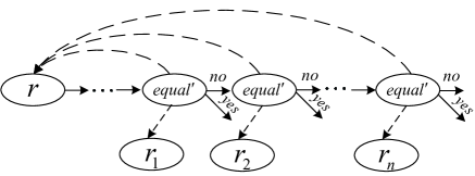
Figure 2: Sub-protocol $f_{mem}$ for decision of set-membership

Embedding the multiset state. For the multiset state, we keep a multiset $S^{MS}$ of the current ground facts. In the execution model, we need to encode the multiset state construct $[L]-[e]\rightarrow[R];P$ by using CoSP sub-protocol $f_{match}$. As in Fig. 1, the SAPIC process tries to match each fact in the sequence $L$ to the ground facts in $S^{MS}$ and, if successful, adds the corresponding instance of facts $R$ to $S^{MS}$. We denote by $fv(L)$ the set of variables in $L$ that are not under the scope of a previous binder. The variables $x\in fv(L)$ should be bound by the pattern matching. For the reason of efficiency, we store the arguments of ground facts in $S^{MS}$ as CoSP-terms rather than $\pi$-terms, as we have done in the case of functional state. $S^{MS}$ can only be altered using the multiset state construct $[L]-[e]\rightarrow[R];P$. Given a closed SAPIC process, the maximum length of $R$ (counted by the number of fact symbols in $R$) is a constant value. In each execution step, the multiset state construct can proceed at most once. Thus the size of $S^{MS}$ is bounded by a polynomial in the number of execution steps (taken CoSP-terms as blackboxes).

When designing the sub-protocol $f_{match}$ for the multiset state construct, we should solve the pattern matching problem, which is similar to the previous one in the input construct. To solve this problem, we need to do our second restriction. In the multiset state construct $[L]-[e]\rightarrow[R];P$, we require that: (i) it is well-formed (Definition 12 in [20]); (ii) $\forall F(M_{1},...,M_{n})\in L$, either $M_{i}\in fv(L)$ or $fv(M_{i})=\emptyset$ for all $1\leq i\leq n$. It means that the free variables of $L$ can only occur as the arguments of the facts in $L$. By (i), the well-formed requirement, we have $fv(R)\subseteq fv(L)$. Thus all the facts added into the current multiset state $S^{MS}$ are ground. By (ii), we can match each variable in $fv(L)$ to the corresponding arguments of the ground facts in $S^{MS}$ and find the substitution $\tau$ for $fv(L)$ in the execution. Note that our second restriction is necessary for the CS results. Otherwise, if we allow the free variables in $fv(L)$ occur as the subterms of the arguments of facts, it might lead to a mismatch case as we have described in the input construct.

The second restriction does not make the multiset state construct useless. All the examples in [20] using this construct meet our requirements. Moreover, this style of state manipulation is the underlying specification language of the tamarin tool [18]. Even considering our restriction, the tamarin tool is still useful to model security protocols. The example is the NAXOS protocol for the eCK model formalized in [18].

In the following, we will give out the sub-protocol $f_{match}$ of the pattern matching. Since $f_{match}$ is plugged in the execution model of SAPIC, it assumes an initial protocol state which includes an environment $\eta$, an interpretation $\mu$, and a multiset $S^{MS}$ of the current ground facts. For each multiset state construct $[L]-[e]\rightarrow[R]$, $f_{match}$ tries to find a substitution $\tau^{\prime}$ from $fv(L)$ to CoSP-terms, such that $lfacts(L)\eta^{\prime}\mu\subseteq^{\#}S^{MS}$ and $pfacts(L)\eta^{\prime}\mu\subset S^{MS}$, where $\eta^{\prime}=\eta\cup\tau^{\prime}$. For simplicity, we denote by $f/(n,k)$ a $\pi$-fact such that $f/(n,k)=F(M_{1},...,M_{k})\in\mathcal{F}$ and $\{M_{i}\}^{k}_{i=1}$ are $\pi$-terms including $n$ variables. A $\pi$-fact $f/(0,k)$ is ground.

Definition 8 (Sub-protocol of Pattern Matching). Let $\eta$ be a partial function mapping variables to CoSP-terms, let $\mu$ be a partial function mapping $\pi$-names to CoSP-terms, let $S^{MS}$ be a multiset of facts whose arguments are CoSP-terms. Let $[L]-[e]\rightarrow[R];P$ be a multiset state construct with our restriction. We define the sub-protocol $f_{match}$ which contains two stages respectively for the pattern matching of linear and persistent facts in $L$:

Start. For stage 1, let $\tau^{\prime}$ be a totally undefined partial function mapping variables to CoSP-terms. Set $S_{rest}:=S^{MS}$. Let $L_{rest}:=lfacts(L)$ and $L_{linear}:=\emptyset$ be two multisets of $\pi$-facts.

Loop. Choose a $\pi$-fact $l/(n,k)\in^{\#}L_{rest}$, match it to all the fact $f\in^{\#}S_{rest}$ with the same fact symbol by performing the following steps i)-iii). If any check in step ii) is failed, choose the next $f\in^{\#}S_{rest}$ to match. If there is no matching with $l/(n,k)$ for any facts in $S_{rest}$, stop and go to the failure-edge.

• For $n$ variables $x_{i}$ in $l/(n,k)$, pick up $x_{i}\notin dom(\eta)\cup dom(\tau^{\prime})$(i.e., the free variables in $l$), set $\tau^{\prime\prime}:=\tau^{\prime}\cup\{x_{i}\mapsto s_{i}|1\leq i\leq n,x_{i}\notin dom(\eta)\cup dom(\tau^{\prime})\}$ by mapping $x_{i}$ to the CoSP-term $s_{i}$ with the same position in $f$. This can be done since we require free variables should be the arguments of facts.

• For $k$ arguments of $l/(n,k)=F(M_{1},...,M_{k})$, use the CoSP computation node to check whether $t_{j}\cong\text{eval}^{CoSP}(M_{j}\eta^{\prime}\mu)$ for $j=1,...,k$, where $t_{j}$ is the argument of $f$ with the same position, $\eta^{\prime}=\eta\cup\tau^{\prime\prime}$. This can be done since $dom(\eta)\cap dom(\tau^{\prime\prime})=\emptyset$.

• If all the checks in step ii) pass, we set $L_{rest}:=L_{rest}\backslash^{\#}\{l/(n,k)\}$, $S_{rest}:=S_{rest}\backslash^{\#}\{f\}$, $L_{linear}:=L_{linear}\cup^{\#}\{l/(n,k)\}$, and $\tau^{\prime}=\tau^{\prime\prime}$. Loop while $L_{rest}\neq\emptyset$.

Stage 2 is similar. We perform the above algorithm of stage 1 without ^#. In the Start, let $\tau^{\prime}$ be the one we have achieved in stage 1, set $L_{rest}:=pfacts(L)$, $S_{rest}:=S^{MS}$, and do not change $S_{rest}$ in step iii) of the Loop. If both the two stages are successful, $f_{match}$ goes to the success-edge.

All the steps in $f_{match}$ can be performed by CoSP nodes. By the conditions in step ii), if successful, $f_{match}$ will find $\tau^{\prime}$ and $\eta^{\prime}=\eta\cup\tau^{\prime}$ such that $lfacts(L)\eta^{\prime}\mu\subseteq^{\#}S^{MS}$ and $pfacts(L)\eta^{\prime}\mu\subset S^{MS}$. Thus we encode the pattern matching of multiset state construct into the CoSP sub-protocol $f_{match}$.

Then we need to explain that the embedding way does not cost unacceptably high. The time complexity of the above sub-protocol (measured by the CoSP nodes) is approximately the size of $S^{MS}$ times the size of $L$. Given a closed SAPIC process, the maximum size of $L$ is a constant number and the size of $S^{MS}$ is polynomial in the execution steps $t$. Thus there exists a polynomial $p$, such that the computation steps of encoding is bounded by $p(t)$.

Now we could give out the definition of computational execution model of SAPIC in Definition 9. It is an interactive machine $Exec_{P_{0}}^{S}(1^{k})$ that executes the SAPIC process and communicates with a probabilistic polynomial-time adversary. The model maintains a protocol state as 6-tuple $(\mathcal{P},\eta,\mu,S,\Lambda,S^{MS})$. The definition of the evaluation context is similar to that of the applied $\pi$ calculus. We write $E[P]=\mathcal{P}\cup\{P\}$.

In order to relate the symbolic and the computational semantics of a SAPIC process, we also define an additional symbolic execution for closed SAPIC processes as a technical tool as in [11]. It is a direct analogue of the computational execution model and denoted by $SExec_{P_{0}}^{S}$. The difference between $Exec_{P_{0}}^{S}(1^{k})$ and $SExec_{P_{0}}^{S}$ is that the latter one operates on CoSP-terms rather than bitstrings: It computes CoSP-terms $M\eta\mu$ and $eval^{CoSP}D\eta\mu$ instead of bitstrings ceval${}_{\eta,\mu}(M)$ and ceval${}_{\eta,\mu}(D)$, it compares the CoSP-terms using CoSP-destructor $\cong$ instead of checking for equality of bitstrings, and it chooses a fresh nonce $r\in\textbf{N}_{P}$ instead of choosing a random bitstring $r$ as value for a new protocol name.

Due to the limited space, we merge the Definition 10 of the symbolic execution of SAPIC into the Definition 9 of the computational one. It is marked by $[\![...]\!]$. In the main loop, we only present the cases of SAPIC state constructs. For the standard cases, the execution model performs in the same way as the applied $\pi$ calculus model does.

Definition 9 $[\![$10$]\!]$ (Computational $[\![$Symbolic$]\!]$ Execution of SAPIC). Let $P_{0}$ be a closed SAPIC process (where all bound variables and names are renamed such that they are pairwise distinct and distinct from all unbound ones). Let $\mathcal{A}$ be an interactive machine called the adversary. We define the computational $[\![$symbolic$]\!]$ execution of SAPIC calculus as an interactive machine $Exec_{P_{0}}^{S}(1^{k})$ that takes a security parameter $k$ as argument $[\![$interactive machine $SExec_{P_{0}}^{S}$ that takes no argument$]\!]$ and interacts with $\mathcal{A}$:

Start: Let $\mathcal{P}:=\{P_{0}\}$. Let $\eta$ be a totally undefined partial function mapping $\pi$-variables to bitstrings $[\![$CoSP-terms$]\!]$, let $\mu$ be a totally undefined partial function mapping $\pi$-names to bitstrings $[\![$CoSP-terms$]\!]$, let $S$ be an initially empty set of pairs of bitstrings $[\![$CoSP-terms$]\!]$. Let $S^{MS}$ be an initially empty multiset of facts whose arguments are bitstrings $[\![$CoSP-terms$]\!]$. Let $\Lambda$ be an initially empty set of bitstrings $[\![$CoSP-terms$]\!]$. Let $a_{1},...,a_{n}$ denote the free names in $P_{0}$. Pick $\{r_{i}\}_{i=1}^{n}\in\text{Nonces}_{k}$ at random $[\![$Choose a different $r_{i}\in\textbf{N}_{P}$$]\!]$. Set $\mu:=\mu\cup\{a_{i}:=r_{i}\}_{i=1}^{n}$. Send $(r_{1},...,r_{n})$ to $\mathcal{A}$.

Main loop: Send $\mathcal{P}$ to $\mathcal{A}$ and expect an evaluation context $E$ from the adversary. Distinguish the following cases:

• For the standard cases, the execution model performs the same way as in Definition 5 $[\![$6$]\!]$.

• $\mathcal{P}=E[\text{insert }M,N;P_{1}]$: Set $m:=\text{ceval}_{\eta,\mu}(M),n:=\text{ceval}_{\eta,\mu}(N)$ $[\![m:=\text{eval}^{CoSP}(M\eta\mu),n:=\text{eval}^{CoSP}(N\eta\mu)]\!]$. Plug in $f_{mem}$ to decide if $\exists(r^{\prime},r)\in S,r^{\prime}=m$ $[\![r^{\prime}\cong m]\!]$. For the success-edge, set $\mathcal{P}:=E[P_{1}]$ and $S:=S\backslash\{(r^{\prime},r)\}\cup\{(m,n)\}$. For the failure-edge, set $\mathcal{P}:=E[P_{1}]$ and $S:=S\cup\{(m,n)\}$.

• $\mathcal{P}=E[\text{delete }M;P_{1}]$: Set $m:=\text{ceval}_{\eta,\mu}(M)$ $[\![m:=\text{eval}^{CoSP}(M\eta\mu)]\!]$. Plug in $f_{mem}$ to decide if $\exists(r^{\prime},r)\in S,r^{\prime}=m$ $[\![r^{\prime}\cong m]\!]$. For the success-edge, set $\mathcal{P}:=E[P_{1}]$ and $S:=S\backslash\{(r^{\prime},r)\}$. For the failure-edge, set $\mathcal{P}:=E[P_{1}]$.

• $\mathcal{P}=E[\text{lookup }M\text{ as }x\text{ in }P_{1}\text{ else }P_{2}]$: Set $m:=\text{ceval}_{\eta,\mu}(M)$ $[\![m:=\text{eval}^{CoSP}\\ (M\eta\mu)]\!]$. Plug in $f_{mem}$ to decide if $\exists(r^{\prime},r)\in S,r^{\prime}=m$ $[\![r^{\prime}\cong m]\!]$. For the success-edge, set $\mathcal{P}:=E[P_{1}]$ and $\eta:=\eta\cup\{x:=r\}$. For the failure-edge, set $\mathcal{P}:=E[P_{2}]$.

• $\mathcal{P}=E[\text{lock }M;P_{1}]$: Set $m:=\text{ceval}_{\eta,\mu}(M)$ $[\![m:=\text{eval}^{CoSP}(M\eta\mu)]\!]$. Plug in $f_{mem}$ to decide if $\exists r^{\prime}\in\Lambda,r^{\prime}=m$ $[\![r^{\prime}\cong m]\!]$. For the success-edge, do nothing. For the failure-edge, set $\mathcal{P}:=E[P_{1}]$ and $\Lambda:=\Lambda\cup\{m\}$.

• $\mathcal{P}=E[\text{unlock }M;P_{1}]$: Set $m:=\text{ceval}_{\eta,\mu}(M)$ $[\![m:=\text{eval}^{CoSP}(M\eta\mu)]\!]$. Plug in $f_{mem}$ to decide if $\exists r^{\prime}\in\Lambda,r^{\prime}=m$ $[\![r^{\prime}\cong m]\!]$. For the success-edge, set $\mathcal{P}:=E[P_{1}]$ and $\Lambda:=\Lambda\backslash\{r^{\prime}\}$. For the failure-edge, do nothing.

• $\mathcal{P}=E[[L]-[e]\rightarrow[R];P_{1}]$: Plug in $f_{match}$ to find a substitution $\tau^{\prime}$ from $fv(L)$ to bitstrings $[\![$CoSP-terms$]\!]$, such that $lfacts(L)\eta^{\prime}\mu\subseteq^{\#}S^{MS}$ and $pfacts(L)\eta^{\prime}\mu\subset S^{MS}$, where $\eta^{\prime}=\eta\cup\tau^{\prime}$. For the success-edge, set $\mathcal{P}:=E[P_{1}]$, $S^{MS}:=S^{MS}\backslash^{\#}lfacts(L)\eta^{\prime}\mu\cup R\eta^{\prime}\mu$, $\eta:=\eta^{\prime}$, and raise the event $e$. For the failure-edge, do nothing.

• In all other cases, do nothing.

For a given polynomial-time interactive machine $\mathcal{A}$, a closed SAPIC process $P_{0}$, and a polynomial $p$, let $Events_{\mathcal{A},P_{0},p}^{S}(k)$ be the distribution for the list of events raised within the first $p(k)$ computational steps (jointly counted for $\mathcal{A}(1^{k})$ and $Exec_{P_{0}}^{S}(1^{k})$). Then the computational fulfillment of SAPIC trace properties can be defined as follows.

Definition 11 (Computational SAPIC Trace Properties). Let $P_{0}$ be a closed process, and $p$ a polynomial. We say that $P_{0}$ computationally satisfies a SAPIC trace property $\wp$ if for all polynomial-time interactive machines $\mathcal{A}$ and all polynomials $p$, we have that $\text{Pr}[Events_{\mathcal{A},P_{0},p}^{S}(k)\in\wp]$ is overwhelming in $k$.

Then we should explain that $SExec_{P_{0}}^{S}$ can be realized by a CoSP protocol tree. The state of the machine $SExec_{P_{0}}^{S}$ includes a tuple $(\mathcal{P},\mu,\eta,S,S^{MS},\Lambda)$. It is used as a node identifier. CoSP-terms should be encoded by the indexes in the path from the root to the node in which they were created (or received). The process $\mathcal{P}$, the fact symbols in $S^{MS}$, and the $\pi$-names in $dom(\mu)$ will be encoded as bitstrings. We plug two sub-protocols, $f_{mem}$ and $f_{match}$, into the CoSP protocol respectively for the decision of set-membership in the functional state constructs, and for the pattern matching in the multiset state constructs. We have explained that these two sub-protocols do not introduce an unacceptable cost. The operation of raising event $e$ can be realized using a control node with one successor that sends $(event,e)$ to the adversary. Given a sequence of nodes $\underline{\nu}$, we denote by $events(\underline{\nu})$ the events $\underline{e}$ raised by the event nodes in $\underline{\nu}$. We call this resulting CoSP protocol $\Pi_{P_{0}}^{S}$.

Definition 12. $SExec_{P_{0}}^{S}$ satisfies a SAPIC trace property $\wp$ if in a finite interaction with any Dolev-Yao adversary, the sequence of events raised by $SExec_{P_{0}}^{S}$ is contained in $\wp$.

Before we prove Theorem 1 of the CS result of SAPIC, we first state and prove three lemmas. Lemma 1 relates the computational/symbolic execution of SAPIC calculus and the CoSP protocol $\Pi_{P_{0}}^{S}$. Lemma 2 states that $\Pi_{P_{0}}^{S}$ is efficient. Lemma 3 asserts that the symbolic execution is a safe approximation for SAPIC. Theorem 1 states that the computationally sound implementation of the symbolic model of applied $\pi$ calculus implies the CS result of SAPIC calculus. We present the proofs in Appendix A.

Lemma 1. $SExec_{P_{0}}^{S}$ satisfies a trace property $\wp$ iff $\Pi_{P_{0}}^{S}$ satisfies $events^{-1}(\wp)$. Moreover, $P_{0}$ computationally satisfies $\wp$ iff $(\Pi_{P_{0}}^{S},A)$ computationally satisfies $events^{-1}(\wp)$. Both are in the sense of Definition 2.

Lemma 2. The CoSP protocol $\Pi_{P_{0}}^{S}$ is efficient.

Lemma 3. If a SAPIC closed process $P_{0}$ symbolically satisfies a SAPIC trace property $\wp$ in the sense of Definition 7, then $SExec_{P_{0}}^{S}$ satisfies $\wp$ in the sense of Definition 12.

Theorem 1 (CS in SAPIC). Assume that the computational implementation of the applied $\pi$ calculus is a computationally sound implementation (in the sense of Definition 3) of the symbolic model of applied $\pi$ calculus (Definition 4) for a class P of protocols. If a closed SAPIC process $P_{0}$ symbolically satisfies a SAPIC trace property $\wp$ (Definition 7), and $\Pi_{P_{0}}^{S}\in\textbf{P}$, then $P_{0}$ computationally satisfies $\wp$ (Definition 11).

4 Computational Soundness Result for StatVerif

StatVerif was proposed in [21]. Its process language is an extension of the ProVerif process calculus with only functional state constructs. StatVerif is limited to the verification of secrecy property.

In this section, we first encode the StatVerif processes into a subset of SAPIC processes. Then we prove that our encoding is able to capture secrecy of stateful protocols by using SAPIC trace properties. Finally with the CS result of SAPIC, we can directly obtain the CS result for StatVerif calculus. Note that our encoding way shows the differences between the semantics of state constructs in these two calculi.

Table 3: State constructs of StatVerif calculus

$\langle P,Q\rangle::=$	processes
…	standard processes
$[s\mapsto M]$	initialize
$s:=M;P$	assign
read $s$ as $x;P$	read
lock; $P$	lock state
unlock; $P$	unlock state

Syntax. We first review the StatVerif calculus proposed in [21]. We list the explicit functional state constructs in Table 3. Table 1 and 3 together compose the full syntax of StatVerif calculus. Note that the state constructs are subject to the following two additional restrictions:

• $[s\mapsto M]$ may occur only once for a given cell name $s$, and may occur only within the scope of name restriction, a parallel and a replication.

• For every lock$;P$, the part $P$ of the process must not include parallel or replication unless it is after an unlock construct.

Operational Semantics. A semantic configuration for StatVerif is a tuple $(\tilde{n},\mathcal{S},\mathcal{P},\mathcal{K})$. $\tilde{n}$ is a finite set of names. $\mathcal{S}=\{s_{i}:=M_{i}\}$ is a partial function mapping cell names $s_{i}$ to their associated values $M_{i}$. $\mathcal{P}=\{(P_{1},\beta_{1}),...,(P_{k},\beta_{k})\}$ is a finite multiset of pairs where $P_{i}$ is a process and $\beta_{i}\in\{0,1\}$ is a boolean indicating whether $P_{i}$ has locked the state. For any $1\leq i\leq k$, we have at most one $\beta_{i}=1$. $\mathcal{K}$ is a set of ground terms modeling the messages output to the environment (adversary). The semantics of StatVerif calculus is defined by transition rules on semantic configurations. We do a little change to the original semantics by adding two labelled transitions for the input and output of adversary. With these rules, we can define secrecy property without explicitly considering the adversary processes. We list these two rules and the semantics of state constructs in Fig. 3. The rest are in [21].

$$\left({\tilde{n},\mathcal{S},\mathcal{P}\cup\left\{{\left({[s\mapsto M],0}\right)}\right\},\mathcal{K}}\right) \xrightarrow{{}}\left({\tilde{n},\mathcal{S}\cup\{s:=M\},\mathcal{P},\mathcal{K}}\right){\text{ if }}s\in\tilde{n}{\text{ and }}s\notin dom(\mathcal{S})\hfill$$

$$\left({\tilde{n},\mathcal{S},\mathcal{P}\cup\left\{{\left({s:=N;P,\beta}\right)}\right\},\mathcal{K}}\right) \xrightarrow{{}}\left({\tilde{n},\mathcal{S}\cup\{s:=N\},\mathcal{P}\cup\left\{{\left({P,\beta}\right)}\right\},\mathcal{K}}\right){\text{ if }}s\in dom(\mathcal{S}){\text{ and }}\forall(Q,\beta^{\prime})\in\mathcal{P},\beta^{\prime}=0\hfill$$

$$\left({\tilde{n},\mathcal{S},\mathcal{P}\cup\left\{{\left({\text{read }s\text{ as }x;P,\beta}\right)}\right\},\mathcal{K}}\right) \xrightarrow{{}}\left({\tilde{n},\mathcal{S},\mathcal{P}\cup\left\{{\left({P\{\mathcal{S}(s)/x\},\beta}\right)}\right\},\mathcal{K}}\right){\text{ if }}s\in dom(\mathcal{S}){\text{ and }}\forall(Q,\beta^{\prime})\in\mathcal{P},\beta^{\prime}=0\hfill$$

$$\left({\tilde{n},\mathcal{S},\mathcal{P}\cup\left\{{\left({\text{lock};P,0}\right)}\right\},\mathcal{K}}\right) \xrightarrow{{}}\left({\tilde{n},\mathcal{S},\mathcal{P}\cup\left\{{\left({P,1}\right)}\right\},\mathcal{K}}\right){\text{ if }}\forall(Q,\beta^{\prime})\in\mathcal{P},\beta^{\prime}=0\hfill$$

$$\left({\tilde{n},\mathcal{S},\mathcal{P}\cup\left\{{\left({\text{unlock};P,1}\right)}\right\},\mathcal{K}}\right) \xrightarrow{{}}\left({\tilde{n},\mathcal{S},\mathcal{P}\cup\left\{{\left({P,0}\right)}\right\},\mathcal{K}}\right)\hfill$$

$$\left({\tilde{n},\mathcal{S},\mathcal{P}\cup\left\{{\left({\text{out}(M,N);P,\beta}\right)}\right\},\mathcal{K}}\right) \xrightarrow{{K(N)}}\left({\tilde{n},\mathcal{S},\mathcal{P}\cup\left\{{\left({P,\beta}\right)}\right\},\mathcal{K}\cup\{N\}}\right){\text{ if }}\nu\tilde{n}.\mathcal{K}\vdash M\hfill$$

$$\left({\tilde{n},\mathcal{S},\mathcal{P}\cup\left\{{\left({\text{in}(M,x);P,\beta}\right)}\right\},\mathcal{K}}\right) \xrightarrow{{K(M,N)}}\left({\tilde{n},\mathcal{S},\mathcal{P}\cup\left\{{\left({P\{N/x\},\beta}\right)}\right\},\mathcal{K}}\right){\text{ if }}\nu\tilde{n}.\mathcal{K}\vdash M\text{ and }\nu\tilde{n}.\mathcal{K}\vdash N\hfill$$

Figure 3: The semantics of Statverif

Security Property. StatVerif is limited to the verification of secrecy property. The secrecy property of StatVerif is defined as follows.

Definition 13 (StatVerif Secrecy Property). Let $P$ be a closed StatVerif process, $M$ a message. $P$ preserves the secrecy of $M$ if there exists no trace of the form:

$$\begin{gathered}(\emptyset,\emptyset,\{(P,0)\},fn(P))\xrightarrow{{\alpha}}^{*}(\tilde{n},\mathcal{S},\mathcal{P},\mathcal{K})\text{ where }\nu\tilde{n}.\mathcal{K}\vdash M\\ \end{gathered}$$

In the following, we encode the StatVerif processes into a subset of SAPIC processes and obtain the CS result directly from that of SAPIC, which has been proved in Section 3.2. With this encoding, we can easily embed the StatVerif calculus into the CoSP framework. Thus we do not need to build another computational execution model for StatVerif like what we have done for SAPIC.

There are many differences between the semantics of these two calculi. The lock construct is the place in which they differ the most. For a StatVerif process $P:=\text{lock};P_{1}$, it will lock the state and all the processes in parallel cannot access the current state cells until an unlock in $P_{1}$ is achieved. For a SAPIC process $P:=\text{lock }M;P_{1}$, it will only store the $\pi$-term $M$ in a set $\Lambda$ and make sure it cannot be locked again in another concurrent process $Q:=\text{lock }M^{\prime};Q_{1}$ where $M^{\prime}=_{E}M$ until an unlock construct is achieved. Moreover, the state cells in StatVerif calculus should be initialized before they can be accessed. It is not required in SAPIC. Thus we should do more for a SAPIC process to simulate the state construct in a StatVerif process.

$$\begin{array}[]{l}{\left\lfloor 0\right\rfloor_{0}}=0\quad{\left\lfloor{P|Q}\right\rfloor_{0}}={\left\lfloor P\right\rfloor_{0}}|{\left\lfloor Q\right\rfloor_{0}}\quad{\left\lfloor{\nu n;P}\right\rfloor_{b}}=\nu n;{\left\lfloor P\right\rfloor_{b}}\quad{\left\lfloor{!P}\right\rfloor_{0}}=!{\left\lfloor P\right\rfloor_{0}}\\ {\left\lfloor{{\text{in}}\left({M,x}\right);P}\right\rfloor_{b}}={\text{in}}\left({M,x}\right);{\left\lfloor P\right\rfloor_{b}}\quad{\left\lfloor{{\text{out}}\left({M,N}\right);P}\right\rfloor_{b}}={\text{out}}\left({M,N}\right);{\left\lfloor P\right\rfloor_{b}}\\ {\left\lfloor{{\text{let }}x=D{\text{ in }}P{\text{ else }}Q}\right\rfloor_{b}}={\text{let }}x=D{\text{ in }}{\left\lfloor P\right\rfloor_{b}}{\text{ else }}{\left\lfloor Q\right\rfloor_{b}}\quad{\left\lfloor{{\text{event }}e;P}\right\rfloor_{b}}={\text{event }}e;{\left\lfloor P\right\rfloor_{b}}\\ {\left\lfloor{[s\mapsto M]}\right\rfloor_{0}}={\text{insert }}s,M\\ {\left\lfloor{{\text{lock}};P}\right\rfloor_{0}}={\text{lock }}l;{\left\lfloor P\right\rfloor_{1}}\quad{\left\lfloor{{\text{unlock}};P}\right\rfloor_{1}}={\text{unlock }}l;{\left\lfloor P\right\rfloor_{0}}\\ {\left\lfloor{s:=M;P}\right\rfloor_{b}}=\left\{{\begin{array}[]{*{20}{r}}{{\text{lock }}l;{\text{lookup }}s{\text{ as }}{x_{s}}{\text{ in insert }}s,M;{\text{unlock }}l;{{\left\lfloor P\right\rfloor}_{0}}{\text{ for }}b=0}\\ {{\text{lookup }}s{\text{ as }}{x_{s}}{\text{ in insert }}s,M;{{\left\lfloor P\right\rfloor}_{1}}{\text{ for }}b=1}\\ \text{where }x_{s}\text{ is a fresh variable}\\ \end{array}}\right.\\ {\left\lfloor{{\text{read }}s{\text{ as }}x;P}\right\rfloor_{b}}=\left\{{\begin{array}[]{*{20}{r}}{{\text{lock }}l;{\text{lookup }}s{\text{ as }}x{\text{ in unlock }}l;{{\left\lfloor P\right\rfloor}_{0}}{\text{ for }}b=0}\\ {{\text{lookup }}s{\text{ as }}x{\text{ in }}{{\left\lfloor P\right\rfloor}_{1}}{\text{ for }}b=1}\\ \end{array}}\right.\\ \end{array}$$

Figure 4: Encoding Statverif process

We first define the encoding $\lfloor P\rfloor_{b}$ for StatVerif process $P$ with the boolean $b$ indicating whether $P$ has locked the state. Note that we only need to encode the StatVerif state constructs by using SAPIC functional state constructs. We leave the standard constructs unchanged. For the sake of completeness, we list them all in Fig. 4. The state cell initialization $[s\mapsto M]$ is represented by the construct insert $s,M$. To encode the lock operation, we set a free fresh cell name $l$. The lock is represented by lock $l$ and turning the boolean $b$ from $0$ to $1$. The unlock construct is done in the opposite direction. To write a new value into an unlocked state cell ($s:=M$ for $b=0$), we need to perform 4 steps. We first lock $l$ before the operation. It is to ensure the state is not locked in concurrent processes. We then read the original value in $s$ to ensure $s$ has been initialized. We complete the writing operation by the construct insert $s,M$ and finally unlock $l$. When the state has been locked ($s:=M$ for $b=1$), we omit the contructs lock $l$ and unlock $l$ because it has been locked before and the boolean $b$ could be turned from $1$ to $0$ only by an unlock construct. The reading operation is similar where we bind the value to $x$ instead of a fresh variable $x_{s}$.

Let $O=\left({\tilde{n},\mathcal{S},\mathcal{P},\mathcal{K}}\right)$ be a StatVerif semantic configuration where $\mathcal{P}=\{(P_{i},\beta_{i})\}_{i=1}^{k}$ and $\beta_{i}\in\{0,1\}$ indicating whether $P_{i}$ has locked the state. We define the encoding $\lfloor O\rfloor$ as SAPIC semantic configuration.

$$\begin{array}[]{c}\left\lfloor O\right\rfloor=\left\{{\begin{array}[]{*{20}{r}}{\left({\tilde{n},\mathcal{S},\emptyset,\{\lfloor P_{i}\rfloor_{\beta_{i}}\}_{i=1}^{k},\mathcal{K},\left\{l\right\}}\right)}{\text{ if }}\exists(P_{i},\beta_{i})\in\mathcal{P},\beta_{i}=1,\\ {\left({\tilde{n},\mathcal{S},\emptyset,\{\lfloor P_{i}\rfloor_{\beta_{i}}\}_{i=1}^{k},\mathcal{K},\emptyset}\right)}{\text{ if }}\forall(P_{i},\beta_{i})\in\mathcal{P},\beta_{i}=0.\\ \end{array}}\right.\end{array}$$

Before we prove Lemma 6 that our encoding is able to capture secrecy of StatVerif process, we provide Lemma 4 and Lemma 5 to explain that the encoding SAPIC process can simulate the encoded StatVerif process. Then by Theorem 2 we obtain the CS result of StatVerif. The proofs are in Appendix B.

Lemma 4. Let $O_{1}$ be a StatVerif semantic configuration. If $O_{1}\xrightarrow{\alpha}O_{2}$, then $\lfloor O_{1}\rfloor\xrightarrow{\alpha}^{*}\lfloor O_{2}\rfloor$.

Lemma 5. Let $O_{1}$ be a StatVerif semantic configuration. If $\lfloor O_{1}\rfloor\xrightarrow{\alpha}O^{\prime}$, then there exists a StatVerif semantic configuration $O_{2}$, such that $O_{1}\xrightarrow{\alpha}^{*}O_{2}$ and that $O^{\prime}=\lfloor O_{2}\rfloor$ or $O^{\prime}\xrightarrow{}^{*}\lfloor O_{2}\rfloor$.

Lemma 6. Let $P_{0}$ be a closed StatVerif process. Let $M$ be a message. Set $P^{\prime}:=\text{in}(attch,x);\text{let }y=equal(x,M)$ in event $NotSecret$, where $x,y$ are two fresh variables that are not used in $P_{0}$, $attch\in\textbf{N}_{E}$ is a free channel name which is known by the adversary. We set $\wp:=\{e|NotSecret$ is not in $e\}$. $Q_{0}:=\lfloor P^{\prime}|P_{0}\rfloor_{0}$ is a closed SAPIC process and $\wp$ is a SAPIC trace property. Then we have that $P_{0}$ symbolically preserves the secrecy of $M$ (in the sense of Definition 13) iff $Q_{0}$ symbolically satisfies $\wp$ (in the sense of Definition 7).

Theorem 2 (CS in StatVerif). Assume that the computational implementation of the applied $\pi$ calculus is a computationally sound implementation (Definition 3) of the symbolic model of the applied $\pi$ calculus (Definition 4) for a class P of protocols. For a closed StatVerif process $P_{0}$, we denote by $Q_{0}$ and $\wp$ the same meanings in Lemma 6. Thus if the StatVerif process $P_{0}$ symbolically preserves the secrecy of a message $M$ (Definition 13) and $\Pi_{Q_{0}}^{S}\in\textbf{P}$, then $Q_{0}$ computationally satisfies $\wp$.

5 Case Study: CS Results of Public-Key Encryption and Signatures

In section 3 and 4, we have embedded the stateful applied $\pi$ calculus used in SAPIC and StatVerif into the CoSP framework. CoSP allows for casting CS proofs in a conceptually modular and generic way: proving $x$ cryptographic primitives sound for $y$ calculi only requires $x+y$ proofs (instead of $x\cdot y$ proofs without this framework). In particular with our results, all CS proofs that have been conducted in CoSP are valid for the stateful applied $\pi$ calculus, and hence accessible to SAPIC and StatVerif.

We exemplify our CS results for stateful applied $\pi$ calculus by providing the symbolic model that is accessible to the two verification tools, SAPIC and StatVerif. We use the CS proofs in [15] with a few changes fitting for the verification mechanism in these tools. The symbolic model allows for expressing public-key encryption and signatures.

Let $\textbf{C}:=\{enc/3,$ $ek/1,$ $dk/1,$ $sig/3,$ $vk/1,$ $sk/1,$ $pair/2,$ $string_{0}/1,$ $string_{1}/1,$ $empty/0,$ $garbageSig/2,$ $garbage/1,$ $garbageEnc/2\}$ be the set of constructors. We require that $\textbf{N}=\textbf{N}_{\textbf{E}}\uplus\textbf{N}_{\textbf{P}}$ for countable infinite sets $\textbf{N}_{\textbf{P}}$ of protocol nonces and $\textbf{N}_{\textbf{E}}$ of attacker nonces. Message type T is the set of all terms $T$ matching the following grammar, where the nonterminal $N$ stands for nonces.

$$T::= enc(ek(N),T,N)|ek(N)|dk(N)|sig(sk(N),T,N)|vk(N)|sk(N)|$$

$$pair(T,T)|S|N|garbage(N)|garbageEnc(T,N)|garbageSig(T,N)$$

$$S::= empty|string_{0}(S)|string_{1}(S)$$

Let $\textbf{D}:=\{dec/2,$ $isenc/1,$ $isek/1,$ $isdk/1,$ $ekof/1,$ $ekofdk/1,$ $verify/2,$ $issig/1,$ $isvk/1,$ $issk/1,$ $vkof/2,$ $vkofsk/1,$ $fst/1,$ $snd/1,$ $unstring_{0}/1,$ $equal/2\}$ be the set of destructors. The full description of all destructor rules is given in [15]. Let $\vdash$ be defined as in Definition 4. Let $\textbf{M}=(\textbf{C},\textbf{N},\textbf{T},\textbf{D},\vdash)$ be the symbolic model.

In StatVerif, the symbolic model M can be directly achieved since the term algebra is inherited from ProVerif, whose CS property has been proved in [15]. In SAPIC, we formalize the symbolic model by a signature $\Sigma:=\textbf{C}\cup\textbf{D}$ with the equational theories expressing the destructor rules. Note that 3 destructor rules are filtered out including: i) $ekofdk(dk(t))=ek(t)$; ii) $vkof(sig(sk(t_{1}),t_{2},t_{3}))=vk(t_{1})$; iii) $vkofsk(sk(t))=vk(t)$, since they are not subterm-convergent, which is required by SAPIC (by verification mechanism of tamarin-prover). Note that these rules are all used to derive the public key. We require that for all the signatures and private keys in communication, they should be accompanied by their public keys. In this way, both the adversary and the protocol will not use these rules. To show the usefulness of our symbolic model in this section, we have verified the left-or-right protocol presented in [21] by using SAPIC and StatVerif. In Appendix C and D, we provide the scripts for the protocol.

To establish CS results, we require the protocols to fulfill several natural conditions with respect to their use of randomness. Protocols that satisfy these protocol conditions are called randomness-safe. Additionally, the cryptographic implementations needs to fulfill certain conditions, e.g., that the encryption scheme is PROG-KDM secure, and the signature scheme is SUF-CMA. Both the protocol conditions and the implementation conditions could be found in [15]. Then we conclude CS for protocols in the stateful applied $\pi$ calculus that use public-key encryption and signatures.

Theorem 3 (CS for Enc. and Signatures in SAPIC and StatVerif). Let M be as defined in this section and $A$ of M be an implementation that satisfies the conditions from above. If a randomness-safe closed SAPIC or StatVerif process $P_{0}$ symbolically satisfies a trace property $\wp$, then $P_{0}$ computationally satisfies $\wp$.

6 Conclusion

In this paper, we present two CS results respectively for the stateful applied $\pi$ calculus used in SAPIC tool and StatVerif tool. We show that the CS results of applied $\pi$ calculus implies the CS results of SAPIC calculus and of StatVerif calculus. Thus for any computationally sound implementation of applied $\pi$ calculus, if the security property of a closed stateful process is verified by SAPIC tool or StatVerif tool, it is also computationally satisfied. The work is conducted within the CoSP framework. We give the embedding from the SAPIC calculus to CoSP protocols. Furthermore, we provide an encoding of the StatVerif processes into a subset of SAPIC processes, which shows the differences between the semantics of these two calculi. As a case study, we provide the CS result for the input languages of StatVerif and SAPIC with public-key encryption and signatures.

Appendix A: Proof of Theorem 1

Lemma 1. $SExec_{P_{0}}^{S}$ satisfies a trace property $\wp$ iff $\Pi_{P_{0}}^{S}$ satisfies $events^{-1}(\wp)$. Moreover, $P_{0}$ computationally satisfies $\wp$ iff $(\Pi_{P_{0}}^{S},A)$ computationally satisfies $events^{-1}(\wp)$. Both are in the sense of Definition 2.

Proof

Since $events^{-1}(\wp)$ is the set of nodes sequences whose raised events sequence are in the trace property set $\wp$. Thus the symbolic case is immediate from the construction of $\Pi_{P_{0}}^{S}$. For the computational case, note that the computational implementation of $P_{0}$ is defined like the symbolic one, except that it uses the implementations of the CoSP-constructors (includes the nonces) and CoSP-destructors (includes destructor $equal^{\prime}$) rather than operate abstractly on CoSP-terms. Thus it is true for the computational case.

Lemma 2. The CoSP protocol $\Pi_{P_{0}}^{S}$ is efficient.

Proof

By construction, given all the node identifiers and the edge labels on the path to a node $N$, there should be a deterministic polynomial-time algorithm that can compute the label of $N$ (the current state of the CoSP protocol). According to the construct of $SExec_{P_{0}}^{S}$, it only needs to prove that the computation steps in each loop is bounded by a polynomial in the loop number. We only consider the state constructs and others are with constant numbers. For the functional state constructs, the number of computation steps in set-membership decision $f_{mem}$ is bounded by the cardinal number of set, which is less than the reduction steps of main process. For the multiset state construct, as we have stated in Section 3.2 that the time complexity for the pattern matching algorithm $f_{match}$ is polynomial in the reduction steps. Thus the computation steps of the algorithm would not grow exponentially.

It is left to show that the length of the node identifier is bounded by a polynomial in the length of the path leading to that node. This is equivalent to showing that the state tuple $(\mathcal{P},\mu,\eta,S,S^{MS},\Lambda)$ of $SExec_{P_{0}}^{S}$ is of polynomial-length (when not counting the length of the representations of the CoSP-terms). For $\mu$, $\eta$, $S$, and $\Lambda$, this is immediately satisfied since they grow by at most one entry in each activation of $SExec_{P_{0}}^{S}$. For $S^{MS}$, we have stated in Section 3.2 that its size is polynomial in the number of reduction steps since we treat the CoSP-terms as black-boxes. At last, we should show that the size of processes $P$ in $\mathcal{P}$ is polynomially bounded. Note the fact that in each activation of $SExec_{P_{0}}^{S}$, processes $P$ either gets smaller, or we have $\mathcal{P}=E[!P_{1}]$ and processes $P$ in $\mathcal{P}$ grow by the size of $P_{1}$, which is bounded by the size of $P_{0}$. Thus the size of processes $P$ in $\mathcal{P}$ is linear in the number of activation of $SExec_{P_{0}}^{S}$.

Lemma 3 (Safe Approximation for SAPIC). If a SAPIC closed process $P_{0}$ symbolically satisfies a SAPIC trace property $\wp$ in the sense of Definition 7, then $SExec_{P_{0}}^{S}$ satisfies $\wp$ in the sense of Definition 12.

Proof

. To show this lemma, it is sufficient to show that if $SExec_{P_{0}}^{S}$ raises events $e_{1},...,e_{n}$, then $\underline{e}$ is a SAPIC event trace of $P_{0}$. Hence, for the following we fix an execution of $SExec_{P_{0}}^{S}$ in interaction with a Dolev-Yao adversary $\mathcal{A}$ in which $SExec_{P_{0}}^{S}$ raises the events $e_{1},...,e_{n}$. We then prove the lemma by showing that there exists a finite sequence $[\mathcal{K}_{1},...,\mathcal{K}_{n}]$ of sets of $\pi$-terms such that $(\emptyset,\emptyset,\emptyset,\{P_{0}\},fn(P_{0}),\emptyset)\xrightarrow{}^{*}\xrightarrow{e_{1}}(\tilde{n}_{1},\mathcal{S}_{1},\mathcal{S}^{MS}_{1},\mathcal{P}_{1},\mathcal{K}_{1},\mathcal{L}_{1})\xrightarrow{}^{*}\xrightarrow{e_{2}}\cdots\xrightarrow{}^{*}\xrightarrow{e_{n}}\\ (\tilde{n}_{m},\mathcal{S}_{m},\mathcal{S}^{MS}_{m},\mathcal{P}_{m},\mathcal{K}_{m},\mathcal{L}_{m}).$

For a given iteration of the main loop of $SExec_{P_{0}}^{S}$, let $(\mathcal{P},\eta,\mu,S,S^{MS},\Lambda)$ denote the corresponding state of $SExec_{P_{0}}^{S}$ at the beginning of that iteration. Let $E$ denote the evaluation context chosen in that iteration. Let $\underline{n}$ be the domain of $\mu$ without the names $r_{1},...,r_{n}$ sent in the very beginning of the execution of $SExec_{P_{0}}^{S}$. $(\mathcal{P}^{\prime},\eta^{\prime},\mu^{\prime},S^{\prime},S^{MS^{\prime}},\Lambda^{\prime})$ and $\underline{n}^{\prime}$ are the corresponding values after that iteration. Let $fromadv$ be the list of terms received from the adversary in that iteration, and let $toadv$ be the list of terms sent to the adversary. By $(\mathcal{P}_{0},\eta_{0},\mu_{0},S_{0},S^{MS}_{0},\Lambda_{0})$ we denote the corresponding values before the first iteration but after the sending of the message $(r_{1},...,r_{n})$, and by $(\mathcal{P}_{*},\eta_{*},\mu_{*},S_{*},S^{MS}_{*},\Lambda_{*})$ and $\underline{n}_{*}$ the values after the last iteration. We call a variable or name used if it occurs in the domain of $\eta_{*}$ or $\mu_{*}$, respectively. Note that $\mu_{0}=(a_{1}\mapsto r_{1},...,a_{n}\mapsto r_{n})$ where $\underline{a}$ are the free names in $P_{0}$, but $\underline{n}_{0}=\emptyset$. Note that $\mathcal{P}$ will never contain unused free variables or names.

Let $K$ denote the list of all CoSP-terms output by $SExec_{P_{0}}^{S}$ up to the current iteration. We encode $K=(t_{1},...,t_{m})$ as a substitution $\varphi$ mapping $x_{i}\mapsto t_{i}$ where $x_{i}$ are arbitrary unused variables. We denote by $K^{\prime},\varphi^{\prime}$, $K_{0},\varphi_{0}$ and $K_{*},\varphi_{*}$ the values of $K,\varphi$ after the current iteration, before the iteration (but after sending $(r_{1},...,r_{n})$), and after the last iteration, respectively. Note that $K_{0}=(r_{1},...,r_{n})$.

Let $\gamma$ be an injective partial function that maps every $N\in\textbf{N}_{E}$ to an unused $\pi$-name, and every $N\in\text{range }\mu_{*}$ to $\mu_{*}^{-1}(N)$. (This is possible because $\text{range }\mu_{*}\subseteq\textbf{N}_{P}$ and $\mu_{*}$ is injective.) We additionally require that all unused $\pi$-names are in $\text{range }\gamma$. (This is possible since both $\textbf{N}_{E}$ and the set of unused $\pi$-names are countably infinite.)

The following claims proposed in [11] can still stick. Note that for any $\pi$-destructor $d$ and any $\pi$-terms $\underline{M}$ with $fv(\underline{M})\in dom(\eta)$ and $fn(\underline{M})\in dom(\mu)$, we have that $M\eta\mu$ are CoSP-terms and $d^{\prime}(M\eta\mu)\gamma=d(M\eta\mu\gamma)$ (where $d^{\prime}$ is as in Section 2.2). Hence for a destructor term $D$ with $fv(D)\subseteq dom(\eta)$ and $fn(D)\subseteq dom(\mu)$, we have $eval^{CoSP}(D\eta\mu)\gamma=eval^{\pi}(D\eta\mu\gamma)$. Since $a\mu\gamma=a$ for all names $a\in dom(\mu)$, $D\eta\mu\gamma=D\eta\gamma$. Since $eval^{CoSP}(D\eta\mu)$ does not contain variables, $eval^{CoSP}(D\eta\mu)=eval^{CoSP}(D\eta\mu)\eta$. Thus for $D$ with $fv(D)\subseteq dom(\eta)$ and $fn(D)\subseteq dom(\mu)$, we have

$$eval^{CoSP}(D\eta\mu)\eta\gamma=eval^{\pi}(D\eta\gamma).$$ (1)

where the left hand side is defined iff the right hand side is defined.

Similarly to (1), if $fv(D)\subseteq dom(\varphi)$ and $fn(D)\subseteq dom(\gamma^{-1})$, we have that $eval^{CoSP}(D\varphi\gamma^{-1})\gamma=eval^{\pi}(D\varphi\gamma)$. For a CoSP-term $t$ with $K\vdash t$, from the definition of $\vdash$ it follows that $t=eval^{CoSP}(D_{t}\varphi\gamma^{-1})$ for some destructor $\pi$-term $D_{t}$ containing only unused names and variables in $dom(\varphi)$ (note that every $N\in\textbf{N}_{E}$ can be expressed as $a\gamma^{-1}$ for some unused $a$). Since all unused names are in $dom(\gamma^{-1})$, we have

$$t\gamma=eval^{CoSP}(D_{t}\varphi\gamma^{-1})\gamma=eval^{\pi}(D_{t}\varphi\gamma).$$ (2)

Given two CoSP-terms $t,u$ such that $equal^{\prime}(t,u)\neq\bot$ and $t$ and $u$ only contain nonces $N\in\textbf{N}_{E}\cup\text{range }\mu_{*}$, by definition of $equal^{\prime}$ and using that $\gamma$ is injective and defined on $\textbf{N}_{E}\cup\text{range }\mu_{*}$, we have $equal^{\prime}(t,u)=equal(t\gamma,u\gamma)\gamma^{-1}$ and hence $equal(t\gamma,u\gamma)\neq\bot$. Hence, for $t,u$ only containing nonces $N\in\textbf{N}_{E}\cup\text{range }\mu_{*}$, we have that

$$equal^{\prime}(t,u)\neq\bot\Leftrightarrow t\gamma=_{E}u\gamma$$ (3)

Claim: The main loop in $SExec_{P_{0}}^{S}$ satisfies that $(\underline{n},S\eta\gamma,S^{MS}\eta\gamma,\mathcal{P}\eta\gamma,K\gamma,\Lambda\eta\gamma)\Rightarrow(\underline{n}^{\prime},S^{\prime}\eta^{\prime}\gamma,S^{MS^{\prime}}\eta^{\prime}\gamma,\mathcal{P}^{\prime}\eta^{\prime}\gamma,K^{\prime}\gamma,\Lambda^{\prime}\eta^{\prime}\gamma)$. Here $\Rightarrow$ denotes $\xrightarrow{e}$ if an event $e$ is raised in the current iteration, and $\xrightarrow{}^{*}$ otherwise. $S\eta\gamma:=\{(r\eta\gamma,r^{\prime}\eta\gamma)|\forall(r,r^{\prime})\in S\}$. $S^{MS}\eta\gamma$ is similar by applying the mapping $\eta\gamma$ to all the arguments of facts in $S^{MS}$.

Assuming that we have shown this claim, it follows that $(\underline{n}_{0},S_{0}\eta_{0}\gamma,S^{MS}_{0}\eta\gamma,\\ \mathcal{P}_{0}\eta_{0}\gamma,K_{0}\gamma,\Lambda_{0}\eta_{0}\gamma)\xrightarrow{}^{*}\xrightarrow{e_{1}}\xrightarrow{}^{*}\xrightarrow{e_{2}}\xrightarrow{}^{*}\cdots\xrightarrow{}^{*}\xrightarrow{e_{n}}$. Since $\eta_{0}=S_{0}=S^{MS}=\underline{n}_{0}=\Lambda_{0}=\emptyset$, $K_{0}\gamma=\underline{a}=fn(P_{0})$ and since $\mathcal{P}_{0}=\{P_{0}\}$ does not contain nonces $N\in\textbf{N}$, we have $\mathcal{P}_{0}\eta_{0}\gamma=\mathcal{P}_{0}$. Then we have that $(\emptyset,\emptyset,\emptyset,\{P_{0}\},fn(P_{0}),\emptyset)\xrightarrow{}^{*}\xrightarrow{e_{1}}\xrightarrow{}^{*}\xrightarrow{e_{2}}\xrightarrow{}^{*}\cdots\xrightarrow{}^{*}\xrightarrow{e_{n}}$. This implies that $\underline{e}$ is a SAPIC event trace of $P_{0}$. It proves this lemma.

It is left to prove the claim. We distinguish the following cases:

i) In the following cases, the adversary chooses to proceed the standard $\pi$-process except for the input and output constructs where $\mathcal{P}=E[\nu a;P_{1}]$, or $\mathcal{P}=E[\text{out}(M_{1},N);P_{1}][\text{in}(M_{2},x);P_{2}]$, or $\mathcal{P}=E[\text{let}{\kern 3.0pt}x=D{\kern 3.0pt}\text{in}{\kern 3.0pt}P_{1}{\kern 3.0pt}\text{else}{\kern 3.0pt}P_{2}]$, or $\mathcal{P}=E[\text{event}{\kern 3.0pt}e;P_{1}]$, or $\mathcal{P}=E[!P_{1}]$. In these cases, we have $S^{\prime}=S$, $S^{MS^{\prime}}=S^{MS}$, $K^{\prime}=K$, $\Lambda^{\prime}=\Lambda$. For all $x\in dom(\eta^{\prime})\backslash dom(\eta)$, we have $x\notin fv(S)\cup fv(\Lambda)\cup fv(S^{MS})$. Thus $S\eta\gamma=S^{\prime}\eta^{\prime}\gamma$, $\Lambda\eta\gamma=\Lambda^{\prime}\eta^{\prime}\gamma$ and $S^{MS}\eta\gamma=S^{MS^{\prime}}\eta^{\prime}\gamma$. According to the proof of Lemma 4 in [11], we have that $(\underline{n},S\eta\gamma,S^{MS}\eta\gamma,\mathcal{P}\eta\gamma,K\gamma,\Lambda\eta\gamma)\Rightarrow(\underline{n}^{\prime},S^{\prime}\eta^{\prime}\gamma,S^{MS^{\prime}}\eta\gamma,\mathcal{P}^{\prime}\eta^{\prime}\gamma,K^{\prime}\gamma,\Lambda^{\prime}\eta^{\prime}\gamma)$.

ii) $\mathcal{P}=E[\text{in}(M,x);P_{1}]$ and $fromadv=(c,m)$ and $eval^{CoSP}M\eta\mu\cong c$: Then $\mathcal{P}^{\prime}=E[P_{1}]$, $K^{\prime}=K$, $S^{\prime}=S$, $S^{MS^{\prime}}=S^{MS}$, $\Lambda^{\prime}=\Lambda$, $\mu^{\prime}=\mu$, and $\eta^{\prime}=\eta\cup\{x:=m\}$. Furthermore, since $SExec_{P_{0}}^{S}$ interacts with a Dolev-Yao adversary, $K\vdash c,m$. By (2), we have $K\gamma\vdash c\gamma,m\gamma$. Since a Dolev-Yao adversary will never derive protocol nonces that have never been sent, we have that only nonces $N\in\textbf{N}_{E}\cup\text{range }\mu$ occur in $c$ and in $M\eta\mu$. Hence with (3), from $M\eta\mu=eval^{CoSP}M\eta\mu\cong c$ it follows that $M\eta\gamma=M\eta\mu\gamma=_{E}c\gamma$. Thus we have

$$\left({\underline{n},S\eta\gamma,S^{MS}\eta\gamma,\mathcal{P}\eta\gamma,K\gamma,\Lambda\eta\gamma}\right)$$

$$= \left({\underline{n},S\eta\gamma,S^{MS}\eta\gamma,\left({E\eta\gamma}\right)\left[\text{in}(M\eta\gamma,x);P_{1}\eta\gamma\right],K\gamma,\Lambda\eta\gamma}\right)$$

$$\to \left({\underline{n},S\eta\gamma,S^{MS}\eta\gamma,\left({E\eta\gamma}\right)\left[P_{1}\eta\gamma\{m\gamma/x\}\right],K\gamma,\Lambda\eta\gamma}\right)$$

$$= \left({\underline{n}^{\prime},S^{\prime}\eta^{\prime}\gamma,S^{MS^{\prime}}\eta^{\prime}\gamma,\mathcal{P}^{\prime}\eta^{\prime}\gamma,K^{\prime}\gamma,\Lambda^{\prime}\eta^{\prime}\gamma}\right)$$

Since we maintain the invariant that all bound variables in $\mathcal{P}$ are distinct from all other variables in $\mathcal{P}$, or $S$, or $\lambda$, or $dom(\eta)$, we have $x\notin fv(E)$, $x\notin S$, $x\notin\lambda$, $x\notin S^{MS}$, and $x\notin dom(\eta)$. Hence $E\eta\gamma=E\eta^{\prime}\gamma$, ${P_{1}}\eta\gamma\{m\gamma/x\}={P_{1}}\eta\{{m/x}\}\gamma={P_{1}}\eta^{\prime}\gamma$, $\Lambda\eta\gamma=\Lambda\eta^{\prime}\gamma$. Thus the last equation is true.

iii) $\mathcal{P}=E[\text{out}(M,N);P_{1}]$ with $t_{M}^{\prime}:=fromadv\cong t_{M}$ and $toadv=t_{N}$ where $t_{M}\cong eval^{CoSP}(M\eta\mu)$ and $t_{N}:=eval^{CoSP}(N\eta\mu)$. Then $K^{\prime}=K\cup\{t_{N}\}$, $\mathcal{P}^{\prime}=E[P_{1}]$, $\eta^{\prime}=\eta$, $\mu^{\prime}=\mu$, $S^{\prime}=S$, $S^{MS^{\prime}}=S^{MS}$, and $\Lambda^{\prime}=\Lambda$. Since $t_{M}^{\prime}$ was sent by the adversary, $K\vdash t_{M}^{\prime}$. According to the Dolev-Yao property, the adversary will never derive protocol nonces that have never been sent, we have that only nonces $N\in\textbf{N}_{E}\cup\text{range }\mu$ occur in $t_{M}^{\prime}$ and $M\eta\mu$. Hence with (3), from $t_{M}^{\prime}\cong t_{M}$ it follows that $M\eta\gamma=M\eta\mu\gamma=t_{M}\gamma=_{E}t_{M}^{\prime}\gamma$, and that $N\eta\gamma=t_{N}\gamma$. Thus $K\gamma\vdash M\eta\gamma$, and $K^{\prime}\gamma=K\gamma\cup\{t_{N}\gamma\}=K\gamma\cup\{N\eta\gamma\}$. We have that

$$\left({\underline{n},S\eta\gamma,S^{MS}\eta\gamma,\mathcal{P}\eta\gamma,K\gamma,\Lambda\eta\gamma}\right)$$

$$= \left({\underline{n},S\eta\gamma,S^{MS}\eta\gamma,\left({E\eta\gamma}\right)\left[\text{out}(M\eta\gamma,N\eta\gamma);P_{1}\eta\gamma\right],K\gamma,\Lambda\eta\gamma}\right)$$

$$\to \left({\underline{n},S\eta\gamma,S^{MS}\eta\gamma,\left({E\eta\gamma}\right)\left[P_{1}\eta\gamma\right],K\gamma\cup\{N\eta\gamma\},\Lambda\eta\gamma}\right)$$

$$= \left({\underline{n}^{\prime},S^{\prime}\eta^{\prime}\gamma,S^{MS^{\prime}}\eta^{\prime}\gamma,\mathcal{P}^{\prime}\eta^{\prime}\gamma,K^{\prime}\gamma,\Lambda^{\prime}\eta^{\prime}\gamma}\right)$$

iv) $\mathcal{P}=E[\text{insert }M,N;P_{1}]$ with $t_{M}=eval^{CoSP}(M\eta\mu)$, $t_{N}=eval^{CoSP}(N\eta\mu)$, and $\exists(r,r^{\prime})\in S$ such that $r\cong t_{M}$. Then $K^{\prime}=K,\mathcal{P}^{\prime}=E[P_{1}],\eta^{\prime}=\eta,\mu^{\prime}=\mu,S^{\prime}=S\backslash\{(r,r^{\prime})\}\cup\{(t_{M},t_{N})\},S^{MS^{\prime}}=S^{MS},\Lambda^{\prime}=\Lambda$. By (1), $t_{M}\eta\gamma=eval^{\pi}(M\eta\gamma)=M\eta\gamma$, $t_{N}\eta\gamma=N\eta\gamma$. $r\cong t_{M}$ implies $r\eta\cong t_{M}\eta$. Since a Dolev-Yao adversary will never derive protocol nonces that have never been sent, we have that only nonces $N\in\textbf{N}_{E}\cup\text{range }\mu$ occur in $r\eta$ and $t_{M}\eta$. By (3), $M\eta\gamma=t_{M}\eta\gamma=r\eta\gamma\in dom(S)\eta\gamma$. Thus we have

$$\left({\underline{n},S\eta\gamma,S^{MS}\eta\gamma,\mathcal{P}\eta\gamma,K\gamma,\Lambda\eta\gamma}\right)$$

$$= \left({\underline{n},S\eta\gamma,S^{MS}\eta\gamma,\left({E\eta\gamma}\right)\left[\text{insert }M\eta\gamma,N\eta\gamma;P_{1}\eta\gamma\right],K\gamma,\Lambda\eta\gamma}\right)$$

$$\to (\underline{n},S\eta\gamma\backslash\{(r\eta\gamma,r^{\prime}\eta\gamma)\}\cup\{M\eta\gamma\mapsto N\eta\gamma\},S^{MS}\eta\gamma,\left({E\eta\gamma}\right)\left[P_{1}\eta\gamma\right],K\gamma,\Lambda\eta\gamma)$$

$$= (\underline{n}^{\prime},\left(S\backslash\{(r,r^{\prime})\}\cup\{(t_{M},t_{N})\}\right)\eta\gamma,S^{MS^{\prime}}\eta^{\prime}\gamma,)\mathcal{P}^{\prime}\eta^{\prime}\gamma,K^{\prime}\gamma,\Lambda^{\prime}\eta^{\prime}\gamma)$$

$$= \left({\underline{n}^{\prime},S^{\prime}\eta^{\prime}\gamma,S^{MS^{\prime}}\eta^{\prime}\gamma,\mathcal{P}^{\prime}\eta^{\prime}\gamma,K^{\prime}\gamma,\Lambda^{\prime}\eta^{\prime}\gamma}\right)$$

v) $\mathcal{P}=E[\text{insert }M,N;P_{1}]$ with $t_{M}=eval^{CoSP}(M\eta\mu)$, $t_{N}=eval^{CoSP}(N\eta\mu)$, and $\forall(r,r^{\prime})\in S$, $r\ncong t_{M}$. Then $K^{\prime}=K,\mathcal{P}^{\prime}=E[P_{1}],\eta^{\prime}=\eta,\mu^{\prime}=\mu,S^{\prime}=S\cup\{(t_{M},t_{N})\},S^{MS^{\prime}}=S^{MS},\Lambda^{\prime}=\Lambda$. By (1), $t_{M}\eta\gamma=eval^{\pi}(M\eta\gamma)=M\eta\gamma$, $t_{N}\eta\gamma=N\eta\gamma$. $r\ncong t_{M}$ implies $r\eta\ncong t_{M}\eta$. Since a Dolev-Yao adversary will never derive protocol nonces that have never been sent, we have that only nonces $N\in\textbf{N}_{E}\cup\text{range }\mu$ occur in $r\eta$ and $t_{M}\eta$. By (3), $M\eta\gamma=t_{M}\eta\gamma\neq r\eta\gamma$ for all $r\eta\gamma\in dom(S)\eta\gamma$. Thus we have

$$\left({\underline{n},S\eta\gamma,S^{MS}\eta\gamma,\mathcal{P}\eta\gamma,K\gamma,\Lambda\eta\gamma}\right)$$

$$= \left({\underline{n},S\eta\gamma,S^{MS}\eta\gamma,\left({E\eta\gamma}\right)\left[\text{insert }M\eta\gamma,N\eta\gamma;P_{1}\eta\gamma\right],K\gamma,\Lambda\eta\gamma}\right)$$

$$\to \left({\underline{n},S\eta\gamma\cup\{(M\eta\gamma,N\eta\gamma)\},S^{MS}\eta\gamma,\left({E\eta\gamma}\right)\left[P_{1}\eta\gamma\right],K\gamma,\Lambda\eta\gamma}\right)$$

$$= \left({\underline{n}^{\prime},\left(S\cup\{(t_{M},t_{N})\}\right)\eta\gamma,S^{MS^{\prime}}\eta^{\prime}\gamma,\mathcal{P}^{\prime}\eta^{\prime}\gamma,K^{\prime}\gamma,\Lambda^{\prime}\eta^{\prime}\gamma}\right)$$

$$= \left({\underline{n}^{\prime},S^{\prime}\eta^{\prime}\gamma,S^{MS^{\prime}}\eta^{\prime}\gamma,\mathcal{P}^{\prime}\eta^{\prime}\gamma,K^{\prime}\gamma,\Lambda^{\prime}\eta^{\prime}\gamma}\right)$$

vi) $\mathcal{P}=E[\text{delete }M;P_{1}]$ with $t_{M}=eval^{CoSP}(M\eta\mu)$, and $\exists(r,r^{\prime})\in S$ such that $r\cong t_{M}$. Then $K^{\prime}=K,\mathcal{P}^{\prime}=E[P_{1}],\eta^{\prime}=\eta,\mu^{\prime}=\mu,S^{\prime}=S\backslash\{(r,r^{\prime})\},S^{MS^{\prime}}=S^{MS},\Lambda^{\prime}=\Lambda$. By (1), $t_{M}\eta\gamma=eval^{\pi}(M\eta\gamma)=M\eta\gamma$. $r\cong t_{M}$ implies $r\eta\cong t_{M}\eta$. Since a Dolev-Yao adversary will never derive protocol nonces that have never been sent, we have that only nonces $N\in\textbf{N}_{E}\cup\text{range }\mu$ occur in $r\eta$ and $t_{M}\eta$. By (3), $M\eta\gamma=t_{M}\eta\gamma=r\eta\gamma\in dom(S)\eta\gamma$. Thus we have

$$\left({\underline{n},S\eta\gamma,S^{MS}\eta\gamma,\mathcal{P}\eta\gamma,K\gamma,\Lambda\eta\gamma}\right)$$

$$= \left({\underline{n},S\eta\gamma,S^{MS}\eta\gamma,\left({E\eta\gamma}\right)\left[\text{delete }M\eta\gamma;P_{1}\eta\gamma\right],K\gamma,\Lambda\eta\gamma}\right)$$

$$\to \left({\underline{n},S\eta\gamma\backslash\{(r\eta\gamma,r^{\prime}\eta\gamma)\},S^{MS}\eta\gamma,\left({E\eta\gamma}\right)\left[P_{1}\eta\gamma\right],K\gamma,\Lambda\eta\gamma}\right)$$

$$= \left({\underline{n}^{\prime},\left(S\backslash\{(r,r^{\prime})\}\right)\eta\gamma,S^{MS^{\prime}}\eta^{\prime}\gamma,\mathcal{P}^{\prime}\eta^{\prime}\gamma,K^{\prime}\gamma,\Lambda^{\prime}\eta^{\prime}\gamma}\right)$$

$$= \left({\underline{n}^{\prime},S^{\prime}\eta^{\prime}\gamma,S^{MS^{\prime}}\eta^{\prime}\gamma,\mathcal{P}^{\prime}\eta^{\prime}\gamma,K^{\prime}\gamma,\Lambda^{\prime}\eta^{\prime}\gamma}\right)$$

vii) $\mathcal{P}=E[\text{delete }M;P_{1}]$ with $t_{M}=eval^{CoSP}(M\eta\mu)$, and $\forall(r,r^{\prime})\in S$, $r\ncong t_{M}$. Then $K^{\prime}=K,\mathcal{P}^{\prime}=E[P_{1}],\eta^{\prime}=\eta,\mu^{\prime}=\mu,S^{\prime}=S,S^{MS^{\prime}}=S^{MS},\Lambda^{\prime}=\Lambda$. By (1), $t_{M}\eta\gamma=eval^{\pi}(M\eta\gamma)=M\eta\gamma$. $r\ncong t_{M}$ implies $r\eta\ncong t_{M}\eta$. Since a Dolev-Yao adversary will never derive protocol nonces that have never been sent, we have that only nonces $N\in\textbf{N}_{E}\cup\text{range }\mu$ occur in $r\eta$ and $t_{M}\eta$. By (3), $M\eta\gamma=t_{M}\eta\gamma\neq r\eta\gamma$ for all $r\eta\gamma\in dom(S)\eta\gamma$. Thus we have

$$\left({\underline{n},S\eta\gamma,S^{MS}\eta\gamma,\mathcal{P}\eta\gamma,K\gamma,\Lambda\eta\gamma}\right)$$

$$= \left({\underline{n},S\eta\gamma,S^{MS}\eta\gamma,\left({E\eta\gamma}\right)\left[\text{delete }M\eta\gamma;P_{1}\eta\gamma\right],K\gamma,\Lambda\eta\gamma}\right)$$

$$\to \left({\underline{n},S\eta\gamma,S^{MS}\eta\gamma,\left({E\eta\gamma}\right)\left[P_{1}\eta\gamma\right],K\gamma,\Lambda\eta\gamma}\right)$$

$$= \left({\underline{n}^{\prime},S^{\prime}\eta^{\prime}\gamma,S^{MS^{\prime}}\eta^{\prime}\gamma,\mathcal{P}^{\prime}\eta^{\prime}\gamma,K^{\prime}\gamma,\Lambda^{\prime}\eta^{\prime}\gamma}\right)$$

viii) $\mathcal{P}=E[\text{lookup }M\text{ as }x\text{ in }P_{1}\text{ else }P_{2}]$ with $t_{M}=eval^{CoSP}(M\eta\mu)$, and $\exists(r,r^{\prime})\in S$ such that $r\cong t_{M}$. Then $K^{\prime}=K,\mathcal{P}^{\prime}=E[P_{1}],\eta^{\prime}=\eta\cup\{x:=r^{\prime}\},\mu^{\prime}=\mu,S^{\prime}=S,S^{MS^{\prime}}=S^{MS},\Lambda^{\prime}=\Lambda$. By (1), $t_{M}\eta\gamma=eval^{\pi}(M\eta\gamma)=M\eta\gamma$. $r\cong t_{M}$ implies $r\eta\cong t_{M}\eta$. Since a Dolev-Yao adversary will never derive protocol nonces that have never been sent, we have that only nonces $N\in\textbf{N}_{E}\cup\text{range }\mu$ occur in $r\eta$ and $t_{M}\eta$. By (3), $M\eta\gamma=t_{M}\eta\gamma=r\eta\gamma\in dom(S)\eta\gamma$. Thus we have

$$\left({\underline{n},S\eta\gamma,S^{MS}\eta\gamma,\mathcal{P}\eta\gamma,K\gamma,\Lambda\eta\gamma}\right)$$

$$= (\underline{n},S\eta\gamma,S^{MS}\eta\gamma,\left({E\eta\gamma}\right)[\text{lookup }M\eta\gamma\text{ as }x\text{ in }P_{1}\eta\gamma\text{ else }P_{2}\eta\gamma],K\gamma,\Lambda\eta\gamma)$$

$$\to \left({\underline{n},S\eta\gamma,S^{MS}\eta\gamma,\left({E\eta\gamma}\right)\left[P_{1}\eta\gamma\left\{r^{\prime}\eta\gamma/x\right\}\right],K\gamma,\Lambda\eta\gamma}\right)$$

$$= \left({\underline{n}^{\prime},S^{\prime}\eta^{\prime}\gamma,S^{MS^{\prime}}\eta^{\prime}\gamma,\left({E\eta^{\prime}\gamma}\right)\left[P_{1}\eta\gamma\left\{r^{\prime}\eta\gamma/x\right\}\right],K^{\prime}\gamma,\Lambda^{\prime}\eta^{\prime}\gamma}\right)$$

$$= \left({\underline{n}^{\prime},S^{\prime}\eta^{\prime}\gamma,S^{MS^{\prime}}\eta^{\prime}\gamma,\mathcal{P}^{\prime}\eta^{\prime}\gamma,K^{\prime}\gamma,\Lambda^{\prime}\eta^{\prime}\gamma}\right)$$

Since we maintain the invariant that all bound variables in $P_{0}$ are distinct from all other variables in $P_{0}$, $S$, $\Lambda$, or $dom(\eta)$, we have $x\notin fv(E)\cup fv(S^{\prime})\cup fv(\Lambda)\cup dom(S^{MS})\cup dom(\eta)$. Hence $E\eta\gamma=E\eta^{\prime}\gamma$, $S\eta\gamma=S^{\prime}\eta^{\prime}\gamma$, $S^{MS}\eta\gamma=S^{MS^{\prime}}\eta^{\prime}\gamma$, and $\Lambda\eta\gamma=\Lambda^{\prime}\eta^{\prime}\gamma$. Moreover, $P_{1}\eta\gamma\left\{{r^{\prime}\eta\gamma/x}\right\}={P_{1}}\left\{{x:=r^{\prime}}\right\}\eta\gamma={P_{1}}\eta^{\prime}\gamma$. Thus the last equation is true.

ix) $\mathcal{P}=E[\text{lookup }M\text{ as }x\text{ in }P_{1}\text{ else }P_{2}]$ with $t_{M}=eval^{CoSP}(M\eta\mu)$, and $\forall(r,r^{\prime})\in S$, $r\ncong t_{M}$. Then $K^{\prime}=K,\mathcal{P}^{\prime}=E[P_{2}],\eta^{\prime}=\eta,\mu^{\prime}=\mu,S^{\prime}=S,S^{MS^{\prime}}=S^{MS},\Lambda^{\prime}=\Lambda$. By (1), $t_{M}\eta\gamma=eval^{\pi}(M\eta\gamma)=M\eta\gamma$. $r\ncong t_{M}$ implies $r\eta\ncong t_{M}\eta$. Since a Dolev-Yao adversary will never derive protocol nonces that have never been sent, we have that only nonces $N\in\textbf{N}_{E}\cup\text{range }\mu$ occur in $r\eta$ and $t_{M}\eta$. By (3), $M\eta\gamma=t_{M}\eta\gamma\neq r\eta\gamma$ for all $r\eta\gamma\in dom(S)\eta\gamma$. Thus we have

$$\left({\underline{n},S\eta\gamma,S^{MS}\eta\gamma,\mathcal{P}\eta\gamma,K\gamma,\Lambda\eta\gamma}\right)$$

$$= (\underline{n},S\eta\gamma,S^{MS}\eta\gamma,\left({E\eta\gamma}\right)[\text{lookup }M\eta\gamma\text{ as }x\text{ in }P_{1}\eta\gamma\text{ else }P_{2}\eta\gamma],K\gamma,\Lambda\eta\gamma)$$

$$\to \left({\underline{n},S\eta\gamma,S^{MS}\eta\gamma,\left({E\eta\gamma}\right)\left[P_{2}\eta\gamma\right],K\gamma,\Lambda\eta\gamma}\right)$$

$$= \left({\underline{n}^{\prime},S^{\prime}\eta^{\prime}\gamma,S^{MS^{\prime}}\eta^{\prime}\gamma,\mathcal{P}^{\prime}\eta^{\prime}\gamma,K^{\prime}\gamma,\Lambda^{\prime}\eta^{\prime}\gamma}\right)$$

x) $\mathcal{P}=E[\text{lock }M;P_{1}]$ with $t_{M}=eval^{CoSP}(M\eta\mu)$, and $\forall r\in\Lambda$, $r\ncong t_{M}$. Then $K^{\prime}=K,\mathcal{P}^{\prime}=E[P_{1}],\eta^{\prime}=\eta,\mu^{\prime}=\mu,S^{\prime}=S,S^{MS^{\prime}}=S^{MS},\Lambda^{\prime}=\Lambda\cup\{t_{M}\}$. By (1), $t_{M}\eta\gamma=eval^{\pi}(M\eta\gamma)=M\eta\gamma$. $r\ncong t_{M}$ implies $r\eta\ncong t_{M}\eta$. Since a Dolev-Yao adversary will never derive protocol nonces that have never been sent, we have that only nonces $N\in\textbf{N}_{E}\cup\text{range }\mu$ occur in $r\eta$ and $t_{M}\eta$. By (3), $M\eta\gamma=t_{M}\eta\gamma\neq r\eta\gamma$ for all $r\eta\gamma\in\Lambda\eta\gamma$. Thus we have

$$\left({\underline{n},S\eta\gamma,S^{MS}\eta\gamma,\mathcal{P}\eta\gamma,K\gamma,\Lambda\eta\gamma}\right)$$

$$= \left({\underline{n},S\eta\gamma,S^{MS}\eta\gamma,\left({E\eta\gamma}\right)\left[\text{lock }M\eta\gamma;P_{1}\eta\gamma\right],K\gamma,\Lambda\eta\gamma}\right)$$

$$\to \left({\underline{n},S\eta\gamma,S^{MS}\eta\gamma,\left({E\eta\gamma}\right)\left[P_{1}\eta\gamma\right],K\gamma,\Lambda\eta\gamma\cup\{M\eta\gamma\}}\right)$$

$$= \left({\underline{n},S\eta\gamma,S^{MS}\eta\gamma,\left({E\eta\gamma}\right)\left[P_{1}\eta\gamma\right],K\gamma,\Lambda\eta\gamma\cup\{t_{M}\eta\gamma\}}\right)$$

$$= \left({\underline{n}^{\prime},S^{\prime}\eta^{\prime}\gamma,S^{MS^{\prime}}\eta^{\prime}\gamma,\mathcal{P}^{\prime}\eta^{\prime}\gamma,K^{\prime}\gamma,\Lambda^{\prime}\eta^{\prime}\gamma}\right)$$

xi) $\mathcal{P}=E[\text{unlock }M;P_{1}]$ with $t_{M}=eval^{CoSP}(M\eta\mu)$, and $\exists r\in\Lambda$ such that $r\cong t_{M}$. Then $K^{\prime}=K,\mathcal{P}^{\prime}=E[P_{1}],\eta^{\prime}=\eta,\mu^{\prime}=\mu,S^{\prime}=S,S^{MS^{\prime}}=S^{MS},\Lambda^{\prime}=\Lambda\backslash\{r\}$. By (1), $t_{M}\eta\gamma=eval^{\pi}(M\eta\gamma)=M\eta\gamma$. $r\cong t_{M}$ implies $r\eta\cong t_{M}\eta$. Since a Dolev-Yao adversary will never derive protocol nonces that have never been sent, we have that only nonces $N\in\textbf{N}_{E}\cup\text{range }\mu$ occur in $r\eta$ and $t_{M}\eta$. By (3), $M\eta\gamma=t_{M}\eta\gamma=r\eta\gamma\in\Lambda\eta\gamma$. Thus we have

$$\left({\underline{n},S\eta\gamma,S^{MS}\eta\gamma,\mathcal{P}\eta\gamma,K\gamma,\Lambda\eta\gamma}\right)$$

$$= \left({\underline{n},S\eta\gamma,S^{MS}\eta\gamma,\left({E\eta\gamma}\right)\left[\text{unlock }M\eta\gamma;P_{1}\eta\gamma\right],K\gamma,\Lambda\eta\gamma}\right)$$

$$\to \left({\underline{n},S\eta\gamma,S^{MS}\eta\gamma,\left({E\eta\gamma}\right)\left[P_{1}\eta\gamma\right],K\gamma,\Lambda\eta\gamma\backslash\{M\eta\gamma\}}\right)$$

$$= \left({\underline{n},S\eta\gamma,S^{MS}\eta\gamma,\left({E\eta\gamma}\right)\left[P_{1}\eta\gamma\right],K\gamma,\Lambda\eta\gamma\backslash\{t_{M}\eta\gamma\}}\right)$$

$$= \left({\underline{n}^{\prime},S^{\prime}\eta^{\prime}\gamma,S^{MS^{\prime}}\eta^{\prime}\gamma,\mathcal{P}^{\prime}\eta^{\prime}\gamma,K^{\prime}\gamma,\Lambda^{\prime}\eta^{\prime}\gamma}\right)$$

xii) $\mathcal{P}=E[[L]-[e]\rightarrow[R];P_{1}]$ with $\tau^{\prime}:=\{x_{i}\mapsto s_{i}\}$ is a substitution found by the pattern matching algorithm in $SExec_{P_{0}}^{S}$, and such that $lfacts(L)(\eta\cup\tau^{\prime})\mu\subseteq^{\#}{S^{MS}},pfacts(L)(\eta\cup\tau^{\prime})\mu\subset{S^{MS}}$. Then $K^{\prime}=K,\mathcal{P}^{\prime}=E[P_{1}],\eta^{\prime}=\eta\cup\tau^{\prime},\mu^{\prime}=\mu,S^{\prime}=S,S^{MS^{\prime}}=S^{MS}\backslash^{\#}lfacts(L)\eta^{\prime}\mu\cup^{\#}R\eta^{\prime}\mu,\Lambda^{\prime}=\Lambda$. According to the pattern matching sub-protocol $f_{match}$, $\tau^{\prime}$ is grounding for $L$ such that for all symbolic fact $l\in^{\#}lfacts(L)$, there exists a fact $f\in^{\#}S^{MS}$ such that $l\eta^{\prime}\mu=f$, where the equality means that the two symbolic facts have the same fact label, and their arguments (as CoSP-terms) are equal under $\cong$. Then for any $M_{l}$ that is the argument of $l$, let $t_{f}$ be the corresponding one of $f$, by (1) we get $M_{l}\eta^{\prime}\gamma=eval^{CoSP}(M_{l}\eta^{\prime}\mu)\eta^{\prime}\gamma=t_{f}\eta^{\prime}\gamma$. Since all the arguments of $l\eta^{\prime}\gamma$ and $f\eta^{\prime}\gamma$ are equal, we have that $l\eta^{\prime}\gamma=f\eta^{\prime}\gamma$. Hence $lfacts(L\eta^{\prime}\gamma)\subseteq^{\#}S^{MS}\eta^{\prime}\gamma=S^{MS}\eta\gamma$. It is similar to get $pfacts(L\eta^{\prime}\gamma)\subset S^{MS}\eta\gamma$. We set $\tau=\tau^{\prime}\gamma$. Then we have $(L\eta\gamma)\tau=(L\eta\gamma)(\tau^{\prime}\gamma)=L\eta^{\prime}\gamma=(L\eta^{\prime}\mu)\eta^{\prime}\gamma$. The last equation is true since $dom(\eta)\cap dom(\tau^{\prime})=\emptyset$. Similarly, we have $(R\eta\gamma)\tau=R\eta^{\prime}\gamma=(R\eta^{\prime}\mu)\eta^{\prime}\gamma$. Thus we have that

$$\left({\underline{n},S\eta\gamma,S^{MS}\eta\gamma,\mathcal{P}\eta\gamma,K\gamma,\Lambda\eta\gamma}\right)$$

$$= (\underline{n},S\eta\gamma,S^{MS}\eta^{\prime}\gamma,\left({E\eta\gamma}\right)\left[([L\eta\gamma]-[e]\rightarrow[R\eta\gamma]);P_{1}\eta\gamma\right],K\gamma,\Lambda\eta\gamma)$$

$$\to (\underline{n},S\eta\gamma,S^{MS}\eta^{\prime}\gamma\backslash^{\#}lfacts(L\eta\gamma)\tau\cup^{\#}(R\eta\gamma)\tau,\left({E\eta\gamma}\right)\left[(P_{1}\eta\gamma)\tau\right],K\gamma,\Lambda\eta\gamma)$$

$$= (\underline{n},S\eta\gamma,S^{MS}\eta^{\prime}\gamma\backslash^{\#}lfacts(L\eta^{\prime}\mu)\eta^{\prime}\gamma\cup^{\#}(R\eta^{\prime}\mu)\eta^{\prime}\gamma,\left({E\eta\gamma}\right)\left[(P_{1}\eta\gamma)\tau\right],K\gamma,\Lambda\eta\gamma)$$

$$= (\underline{n},S\eta\gamma,S^{MS^{\prime}}\eta^{\prime}\gamma,\left({E\eta\gamma}\right)\left[(P_{1}\eta\gamma)\tau\right],K\gamma,\Lambda\eta\gamma)$$

$$= \left({\underline{n}^{\prime},S^{\prime}\eta^{\prime}\gamma,S^{MS^{\prime}}\eta^{\prime}\gamma,\mathcal{P}^{\prime}\eta^{\prime}\gamma,K^{\prime}\gamma,\Lambda^{\prime}\eta^{\prime}\gamma}\right)$$

Since we maintain the invariant that all bound variables are pairwise distinct, $\forall x\in\tau$, we have $x\notin fv(E)\cup fv(S^{\prime})\cup fv(\Lambda^{\prime})\cup fv(S^{MS})\cup dom(\eta)$. Hence $E\eta\gamma=E\eta^{\prime}\gamma$, $S\eta\gamma=S^{\prime}\eta^{\prime}\gamma$, and $\Lambda\eta\gamma=\Lambda^{\prime}\eta^{\prime}\gamma$. Moreover, we have $(P_{1}\eta\gamma)\tau=(P_{1}\eta\gamma)(\tau^{\prime}\gamma)=P_{1}\eta^{\prime}\gamma$. Thus the last equation is true.

xiii) In all other cases we have $\mathcal{P}^{\prime}=\mathcal{P},K^{\prime}=K,\eta^{\prime}=\eta,\mu^{\prime}=\mu,S^{\prime}=S,S^{MS^{\prime}}=S^{MS},\Lambda^{\prime}=\Lambda$ and that $({\underline{n},S\eta\gamma,S^{MS}\eta\gamma,\mathcal{P}\eta\gamma,K\gamma,\Lambda\eta\gamma})=(\underline{n}^{\prime},\eta^{\prime}\gamma,\\ S^{MS^{\prime}}\eta\gamma,\mathcal{P}^{\prime}\eta^{\prime}\gamma,K^{\prime}\gamma,\Lambda^{\prime}\eta^{\prime}\gamma)$

Theorem 1 (CS in SAPIC). Assume that the computational implementation of the applied $\pi$-calculus is a computationally sound implementation (Definition 3) of the symbolic model of the applied $\pi$-calculus (Definition 4) for a class P of protocols. If a closed SAPIC process $P_{0}$ symbolically satisfies a SAPIC trace property $\wp$ (Definition 7), and $\Pi_{P_{0}}^{S}\in\textbf{P}$, then $P_{0}$ computationally satisfies $\wp$ (Definition 12).

Proof

. Assume that $P_{0}$ symbolically satisfies $\wp$. By lemma 3, $SExec_{P_{0}}^{S}$ satisfies $\wp$. By lemma 1, $\Pi_{P_{0}}^{S}$ symbolically satisfies $events^{-1}(\wp)$. Furthermore, since $\wp$ is an efficiently decidable, prefix closed set, so is $events^{-1}(\wp)$. Thus $events^{-1}(\wp)$ is a CoSP-trace property. By lemma 2, we have that $\Pi_{P_{0}}^{S}$ is an efficient CoSP protocol. By assumption, the computational implementation $A$ of the applied $\pi$-calculus is computationally sound; hence $(\Pi_{P_{0}}^{S},A)$ computationally satisfies $events^{-1}(\wp)$. Using lemma 1, we obtain that $P_{0}$ computationally satisfies $\wp$.

Appendix B: Proof of Theorem 2

Lemma 4. Let $O_{1}$ be a StatVerif semantic configuration. If $O_{1}\xrightarrow{\alpha}O_{2}$, then $\lfloor O_{1}\rfloor\xrightarrow{\alpha}^{*}\lfloor O_{2}\rfloor$.

Proof

. We prove this lemma by induction over the size of the set of processes in $O_{1}$. Let $O_{1}=(\tilde{n},\mathcal{S},\mathcal{P}\cup\{(P_{0},\beta_{0})\},\mathcal{K})$ be a StatVerif semantic configuration, where $\mathcal{P}=\mathop{\cup}\limits_{i=1}^{k}\{(P_{i},\beta_{i})\}$. Assume that $O_{1}\xrightarrow{\alpha}O_{2}$ conducts a reduction on $(P_{0},\beta_{0})$. We distinguish the following cases of $P_{0}$:

i) In the following cases, where $P_{0}=P|0$, or $P_{0}=!P$, or $P_{0}=P|Q$, or $P_{0}=\nu n;P$, or $P_{0}=\text{let }x=D\text{ in }P\text{ else }Q$, or $P_{0}=\text{out}(M,N);P$, or $P_{0}=\text{in}(M,x);P$, or $P_{0}=\text{event }e;P$, we have that $\lfloor P_{0}\rfloor_{\beta_{0}}$ keep the standard constructs unchanged. Thus it is easy to obtain $\lfloor O_{1}\rfloor\xrightarrow{\alpha}^{*}\lfloor O_{2}\rfloor$ where $O_{1}\xrightarrow{\alpha}O_{2}$ conducts a reduction on $(P_{0},\beta_{0})$.

ii) $O_{1}=(\tilde{n},\mathcal{S},\mathcal{P}\cup\{([s\mapsto M],0)\},\mathcal{K})$, $O_{2}=(\tilde{n},\mathcal{S}\cup\{s:=M\},\mathcal{P},\mathcal{K})$, and $s\in\tilde{n},s\notin dom(\mathcal{S})$. Then we have

$$\lfloor O_{1}\rfloor= (\tilde{n},\mathcal{S},\emptyset,\mathop{\cup}\limits_{i=1}^{k}\{\lfloor P_{i}\rfloor_{\beta_{i}}\}\cup\{\text{insert }s,M\},\mathcal{K},\Lambda)$$

$$\to (\tilde{n},\mathcal{S}\cup\{s:=M\},\emptyset,\mathop{\cup}\limits_{i=1}^{k}\{\lfloor P_{i}\rfloor_{\beta_{i}}\},\mathcal{K},\Lambda)$$

$$= \lfloor O_{2}\rfloor$$

where $\Lambda=\{l\}$ if $\exists(P_{i},\beta_{i})\in\mathcal{P},\beta_{i}=1$, or $\Lambda=\emptyset$ if $\forall(P_{i},\beta_{i})\in\mathcal{P},\beta_{i}=0$.

iii) $O_{1}=(\tilde{n},\mathcal{S},\mathcal{P}\cup\{(s:=M;P,0)\},\mathcal{K})$, $O_{2}=(\tilde{n},\mathcal{S}\cup\{s:=M\},\mathcal{P}\cup\{(P,0)\},\mathcal{K})$, and $s\in dom(\mathcal{S}),\forall(P_{i},\beta_{i})\in\mathcal{P},\beta_{i}=0$. Then we have

$$\lfloor O_{1}\rfloor= (\tilde{n},\mathcal{S},\emptyset,\mathop{\cup}\limits_{i=1}^{k}\{\lfloor P_{i}\rfloor_{\beta_{i}}\}\cup\{\text{lock }l;\text{lookup }s\text{ as }x_{s}\text{ in insert }s,M;\text{unlock }l;\lfloor P\rfloor_{0}\},\mathcal{K},\emptyset)$$

$$\to (\tilde{n},\mathcal{S},\emptyset,\mathop{\cup}\limits_{i=1}^{k}\{\lfloor P_{i}\rfloor_{\beta_{i}}\}\cup\{\text{lookup }s\text{ as }x_{s}\text{ in insert }s,M;\text{unlock }l;\lfloor P\rfloor_{0}\},\mathcal{K},\{l\})$$

$$\to (\tilde{n},\mathcal{S},\emptyset,\mathop{\cup}\limits_{i=1}^{k}\{\lfloor P_{i}\rfloor_{\beta_{i}}\}\cup\{\text{insert }s,M;\text{unlock }l;\lfloor P\rfloor_{0}\},\mathcal{K},\{l\})$$

$$\to (\tilde{n},\mathcal{S}\cup\{s:=M\},\emptyset,\mathop{\cup}\limits_{i=1}^{k}\{\lfloor P_{i}\rfloor_{\beta_{i}}\}\cup\{\text{unlock }l;\lfloor P\rfloor_{0}\},\mathcal{K},\{l\})$$

$$\to (\tilde{n},\mathcal{S}\cup\{s:=M\},\emptyset,\mathop{\cup}\limits_{i=1}^{k}\{\lfloor P_{i}\rfloor_{\beta_{i}}\}\cup\{\lfloor P\rfloor_{0}\},\mathcal{K},\emptyset)$$

$$= \lfloor O_{2}\rfloor$$

Note that the second reduction is true because $x_{s}$ is fresh.

iv) $O_{1}=(\tilde{n},\mathcal{S},\mathcal{P}\cup\{(s:=M;P,1)\},\mathcal{K})$, $O_{2}=(\tilde{n},\mathcal{S}\cup\{s:=M\},\mathcal{P}\cup\{(P,1)\},\mathcal{K})$, and $s\in dom(\mathcal{S}),\forall(P_{i},\beta_{i})\in\mathcal{P},\beta_{i}=0$. Then we have

$$\lfloor O_{1}\rfloor= (\tilde{n},\mathcal{S},\emptyset,\mathop{\cup}\limits_{i=1}^{k}\{\lfloor P_{i}\rfloor_{\beta_{i}}\}\cup\{\text{lookup }s\text{ as }x_{s}\text{ in insert }s,M;\lfloor P\rfloor_{1}\},\mathcal{K},\{l\})$$

$$\to (\tilde{n},\mathcal{S},\emptyset,\mathop{\cup}\limits_{i=1}^{k}\{\lfloor P_{i}\rfloor_{\beta_{i}}\}\cup\{\text{insert }s,M;\lfloor P\rfloor_{1}\},\mathcal{K},\{l\})$$

$$\to (\tilde{n},\mathcal{S}\cup\{s:=M\},\emptyset,\mathop{\cup}\limits_{i=1}^{k}\{\lfloor P_{i}\rfloor_{\beta_{i}}\}\cup\{\lfloor P\rfloor_{1}\},\mathcal{K},\{l\})$$

$$= \lfloor O_{2}\rfloor$$

Note that the first reduction is true because $x_{s}$ is fresh.

v) $O_{1}=(\tilde{n},\mathcal{S},\mathcal{P}\cup\{(\text{read }s\text{ as }x;P,0)\},\mathcal{K})$, $O_{2}=(\tilde{n},\mathcal{S},\mathcal{P}\cup\{(P\{\mathcal{S}(s)/x\},0)\},\mathcal{K})$, and $s\in dom(\mathcal{S}),\forall(P_{i},\beta_{i})\in\mathcal{P},\beta_{i}=0$. Then we have

$$\lfloor O_{1}\rfloor= (\tilde{n},\mathcal{S},\emptyset,\mathop{\cup}\limits_{i=1}^{k}\{\lfloor P_{i}\rfloor_{\beta_{i}}\}\cup\{\text{lock }l;\text{lookup }s\text{ as }x\text{ in unlock }l;\lfloor P\rfloor_{0}\},\mathcal{K},\emptyset)$$

$$\to (\tilde{n},\mathcal{S},\emptyset,\mathop{\cup}\limits_{i=1}^{k}\{\lfloor P_{i}\rfloor_{\beta_{i}}\}\cup\{\text{lookup }s\text{ as }x\text{ in unlock }l;\lfloor P\rfloor_{0}\},\mathcal{K},\{l\})$$

$$\to (\tilde{n},\mathcal{S},\emptyset,\mathop{\cup}\limits_{i=1}^{k}\{\lfloor P_{i}\rfloor_{\beta_{i}}\}\cup\{\text{unlock }l;\lfloor P\{\mathcal{S}(s)/x\}\rfloor_{0}\},\mathcal{K},\{l\})$$

$$\to (\tilde{n},\mathcal{S},\emptyset,\mathop{\cup}\limits_{i=1}^{k}\{\lfloor P_{i}\rfloor_{\beta_{i}}\}\cup\{\lfloor P\{\mathcal{S}(s)/x\}\rfloor_{0}\},\mathcal{K},\emptyset)$$

$$= \lfloor O_{2}\rfloor$$

vi) $O_{1}=(\tilde{n},\mathcal{S},\mathcal{P}\cup\{(\text{read }s\text{ as }x;P,1)\},\mathcal{K})$, $O_{2}=(\tilde{n},\mathcal{S},\mathcal{P}\cup\{(P\{\mathcal{S}(s)/x\},1)\},\mathcal{K})$, and $s\in dom(\mathcal{S}),\forall(P_{i},\beta_{i})\in\mathcal{P},\beta_{i}=0$. Then we have

$$\lfloor O_{1}\rfloor= (\tilde{n},\mathcal{S},\emptyset,\mathop{\cup}\limits_{i=1}^{k}\{\lfloor P_{i}\rfloor_{\beta_{i}}\}\cup\{\text{lookup }s\text{ as }x\text{ in }\lfloor P\rfloor_{1}\},\mathcal{K},\{l\})$$

$$\to (\tilde{n},\mathcal{S},\emptyset,\mathop{\cup}\limits_{i=1}^{k}\{\lfloor P_{i}\rfloor_{\beta_{i}}\}\cup\{\lfloor P\{\mathcal{S}(s)/x\}\rfloor_{1}\},\mathcal{K},\{l\})$$

$$= \lfloor O_{2}\rfloor$$

vii) $O_{1}=(\tilde{n},\mathcal{S},\mathcal{P}\cup\{(\text{lock};P,0)\},\mathcal{K})$, $O_{2}=(\tilde{n},\mathcal{S},\mathcal{P}\cup\{(P,1)\},\mathcal{K})$, and $\forall(P_{i},\beta_{i})\in\mathcal{P},\beta_{i}=0$. Then we have

$$\lfloor O_{1}\rfloor= (\tilde{n},\mathcal{S},\emptyset,\mathop{\cup}\limits_{i=1}^{k}\{\lfloor P_{i}\rfloor_{\beta_{i}}\}\cup\{\text{lock }l;\lfloor P\rfloor_{1}\},\mathcal{K},\emptyset)$$

$$\to (\tilde{n},\mathcal{S},\emptyset,\mathop{\cup}\limits_{i=1}^{k}\{\lfloor P_{i}\rfloor_{\beta_{i}}\}\cup\{\lfloor P\rfloor_{1}\},\mathcal{K},\{l\})$$

$$= \lfloor O_{2}\rfloor$$

viii) $O_{1}=(\tilde{n},\mathcal{S},\mathcal{P}\cup\{(\text{unlock};P,1)\},\mathcal{K})$, $O_{2}=(\tilde{n},\mathcal{S},\mathcal{P}\cup\{(P,0)\},\mathcal{K})$, and $\forall(P_{i},\beta_{i})\in\mathcal{P},\beta_{i}=0$. Then we have

$$\lfloor O_{1}\rfloor= (\tilde{n},\mathcal{S},\emptyset,\mathop{\cup}\limits_{i=1}^{k}\{\lfloor P_{i}\rfloor_{\beta_{i}}\}\cup\{\text{unlock }l;\lfloor P\rfloor_{0}\},\mathcal{K},\{l\})$$

$$\to (\tilde{n},\mathcal{S},\emptyset,\mathop{\cup}\limits_{i=1}^{k}\{\lfloor P_{i}\rfloor_{\beta_{i}}\}\cup\{\lfloor P\rfloor_{0}\},\mathcal{K},\emptyset)$$

$$= \lfloor O_{2}\rfloor$$

ix) In all the other cases, there is no reduction for $O_{1}\xrightarrow{\alpha}O_{2}$ that conducts a reduction on $(P_{0},\beta_{0})$.

Lemma 5. Let $O_{1}$ be a StatVerif semantic configuration. If $\lfloor O_{1}\rfloor\xrightarrow{\alpha}O^{\prime}$, then there exists a StatVerif semantic configuration $O_{2}$, such that $O_{1}\xrightarrow{\alpha}^{*}O_{2}$ and that $O^{\prime}=\lfloor O_{2}\rfloor$ or $O^{\prime}\xrightarrow{}^{*}\lfloor O_{2}\rfloor$.

Proof

. We prove this lemma by induction over the size of the set of processes in $\lfloor O_{1}\rfloor$. Let $\lfloor O_{1}\rfloor=(\tilde{n},\mathcal{S},\emptyset,\mathcal{P}^{\prime}\cup\{P_{0}\},\mathcal{K},\Lambda)$ be a SAPIC semantic configuration transformed from a StatVerif semantic configuration, where $\mathcal{P}^{\prime}=\mathop{\cup}\limits_{i=1}^{k}\{P_{i}^{\prime}\}$. Assume that $\lfloor O_{1}\rfloor\xrightarrow{\alpha}O^{\prime}$ conducts a reduction on $P_{0}$. We distinguish the following cases of $P_{0}$:

i) In the following cases, where $P_{0}=P|0$, or $P_{0}=!P$, or $P_{0}=P|Q$, or $P_{0}=\nu n;P$, or $P_{0}=\text{let }x=D\text{ in }P\text{ else }Q$, or $P_{0}=\text{out}(M,N);P$, or $P_{0}=\text{in}(M,x);P$, or $P_{0}=\text{event }e;P$, we have that $\lfloor\cdot\rfloor_{\beta}$ keep the standard constructs unchanged. Thus it is easy to obtain the StatVerif semantic configuration $O_{2}$ such that $O_{1}\xrightarrow{\alpha}O_{2}$ and $O^{\prime}=\lfloor O_{2}\rfloor$.

ii) $\lfloor O_{1}\rfloor=(\tilde{n},\mathcal{S},\emptyset,\mathcal{P}^{\prime}\cup\{\text{insert }s,M;P^{\prime}\},\mathcal{K},\Lambda)$, $O^{\prime}=(\tilde{n},\mathcal{S}\cup\{s:=M\},\emptyset,\mathcal{P}^{\prime}\cup\{P^{\prime}\},\mathcal{K},\Lambda)$. We get $\lfloor O_{1}\rfloor\xrightarrow{\alpha}O^{\prime}$. According to the rules of encoding, we can assume $O_{1}=(\tilde{n},\mathcal{S},\mathcal{P}\cup\{([s\mapsto M],0)\},\mathcal{K})$. Let $O_{2}=(\tilde{n},\mathcal{S}\cup\{s:=M\},\mathcal{P},\mathcal{K})$ be a StatVerif semantic configuration, we have $O^{\prime}=\lfloor O_{2}\rfloor$. It is left to show $O_{1}\xrightarrow{\alpha}O_{2}$. This reduction needs two conditions: $s\in\tilde{n}$ and $s\notin dom(\mathcal{S})$. We get $s\in\tilde{n}$ from the fact that $[s\mapsto M]$ is a process in $O_{1}$ and from the first restriction in the syntax of StatVerif. For $s\notin dom(\mathcal{S})$, we use the disproof method. If $s\in dom(\mathcal{S})$, the first insertion for the state cell $s$ should be performed by the process $\lfloor[s\mapsto N]\rfloor_{0}$ or $\lfloor s:=N;P\rfloor_{\beta}$. The former contradicts the restriction that $[s\mapsto N]$ occurs only once. The latter cannot be the first time to perform the insertion since we set a lookup construct before the insert construct. Thus $s\notin dom(\mathcal{S})$ and we have $O_{1}\xrightarrow{\alpha}O_{2}$.

iii) $\lfloor O_{1}\rfloor=(\tilde{n},\mathcal{S},\emptyset,\mathcal{P}^{\prime}\cup\{\text{unlock }l;P^{\prime}\},\mathcal{K},\{l\})$, $O^{\prime}=(\tilde{n},\mathcal{S},\emptyset,\mathcal{P}^{\prime}\cup\{P^{\prime}\},\mathcal{K},\emptyset)$. We get $\lfloor O_{1}\rfloor\xrightarrow{\alpha}O^{\prime}$. According to the rules of encoding, we can assume $O_{1}=(\tilde{n},\mathcal{S},\mathcal{P}\cup\{(\text{unlock};P,1)\},\mathcal{K})$. Let $O_{2}=(\tilde{n},\mathcal{S},\mathcal{P}\cup\{(P,0)\},\mathcal{K})$ be a StatVerif semantic configuration, we have $O^{\prime}=\lfloor O_{2}\rfloor$ and $O_{1}\xrightarrow{\alpha}O_{2}$.

iv) $\lfloor O_{1}\rfloor=(\tilde{n},\mathcal{S},\emptyset,\mathcal{P}^{\prime}\cup\{\text{lock }l;P^{\prime}\},\mathcal{K},\emptyset)$, $O^{\prime}=(\tilde{n},\mathcal{S},\emptyset,\mathcal{P}^{\prime}\cup\{P^{\prime}\},\mathcal{K},\{l\})$. We get $\lfloor O_{1}\rfloor\xrightarrow{\alpha}O^{\prime}$. According to the rules of encoding, we distinguish 3 cases in the construction of $O_{1}$:

(a) We assume $O_{1}=(\tilde{n},\mathcal{S},\mathcal{P}\cup\{(\text{lock};P,0)\},\mathcal{K})$ and $\forall(P_{i},\beta_{i})\in\mathcal{P},\beta_{i}=0$. Let $O_{2}=(\tilde{n},\mathcal{S},\mathcal{P}\cup\{(P,1)\},\mathcal{K})$ be a StatVerif semantic configuration, we have $O^{\prime}=\lfloor O_{2}\rfloor$ and $O_{1}\xrightarrow{\alpha}O_{2}$.

(b) We assume $O_{1}=(\tilde{n},\mathcal{S},\mathcal{P}\cup\{(s:=M;P,0)\},\mathcal{K})$ and $\forall(P_{i},\beta_{i})\in\mathcal{P},\beta_{i}=0$. According to the rules of encoding, we have $P^{\prime}=\text{lookup }s\text{ as }x_{s}\text{ in insert }s,M;\text{unlock }l;\lfloor P\rfloor_{0}$. If $\mathcal{P}=\{([s\mapsto N],0)\}\cup\mathcal{P}_{1}$, then set $O_{2}=(\tilde{n},\mathcal{S}\cup\{s:=M\},\mathcal{P}_{1}\cup\{(P,0)\},\mathcal{K})$. Otherwise, set $O_{2}=(\tilde{n},\mathcal{S}\cup\{s:=M\},\mathcal{P}\cup\{(P,0)\},\mathcal{K})$. For $\mathcal{P}=\{([s\mapsto N],0)\}\cup\mathcal{P}_{1}$, we have $O_{1}\xrightarrow{}^{*}O_{2}$. It is left to show $O^{\prime}\xrightarrow{}^{*}\lfloor O_{2}\rfloor$. We can assume $\lfloor O_{2}\rfloor=(\tilde{n},\mathcal{S}\cup\{s:=M\},\emptyset,\mathcal{P}_{1}^{\prime}\cup\{\lfloor P\rfloor_{0}\},\mathcal{K},)$ where $\mathcal{P}_{1}^{\prime}=\mathcal{P}^{\prime}\backslash\{\text{insert }s,N\}$. Then we have

$$O^{\prime}= (\tilde{n},\mathcal{S},\emptyset,\mathcal{P}_{1}^{\prime}\cup\{\text{insert }s,N\}\cup\{\text{lookup }s\text{ as }x_{s}\text{ in insert }s,M;\text{unlock }l;\lfloor P\rfloor_{0}\},\mathcal{K},\{l\})$$

$$\to (\tilde{n},\mathcal{S}\cup\{s:=N\},\emptyset,\mathcal{P}_{1}^{\prime}\cup\{\text{lookup }s\text{ as }x_{s}\text{ in insert }s,M;\text{unlock }l;\lfloor P\rfloor_{0}\},\mathcal{K},\{l\})$$

$$\to (\tilde{n},\mathcal{S}\cup\{s:=N\},\emptyset,\mathcal{P}_{1}^{\prime}\cup\{\text{insert }s,M;\text{unlock }l;\lfloor P\rfloor_{0}\},\mathcal{K},\{l\})$$

$$\to (\tilde{n},\mathcal{S}\cup\{s:=M\},\emptyset,\mathcal{P}_{1}^{\prime}\cup\{\text{unlock }l;\lfloor P\rfloor_{0}\},\mathcal{K},\{l\})$$

$$\to (\tilde{n},\mathcal{S}\cup\{s:=M\},\emptyset,\mathcal{P}_{1}^{\prime}\cup\{\lfloor P\rfloor_{0}\},\mathcal{K},\emptyset)$$

$$= \lfloor O_{2}\rfloor$$

For $\{([s\mapsto N],0)\}\notin\mathcal{P}$, we get $s\in dom(\mathcal{S})$ from the restriction of the syntax of $[s\mapsto M]$. Thus we have that $O_{1}\xrightarrow{}^{*}O_{2}$, and that

$$O^{\prime}= (\tilde{n},\mathcal{S},\emptyset,\mathcal{P}^{\prime}\cup\{\text{lookup }s\text{ as }x_{s}\text{ in insert }s,M;\text{unlock }l;\lfloor P\rfloor_{0}\},\mathcal{K},\{l\})$$

$$\to (\tilde{n},\mathcal{S},\emptyset,\mathcal{P}^{\prime}\cup\{\text{insert }s,M;\text{unlock }l;\lfloor P\rfloor_{0}\},\mathcal{K},\{l\})$$

$$\to (\tilde{n},\mathcal{S}\cup\{s:=M\},\emptyset,\mathcal{P}^{\prime}\cup\{\text{unlock }l;\lfloor P\rfloor_{0}\},\mathcal{K},\{l\})$$

$$\to (\tilde{n},\mathcal{S}\cup\{s:=M\},\emptyset,\mathcal{P}^{\prime}\cup\{\lfloor P\rfloor_{0}\},\mathcal{K},\emptyset)$$

$$= \lfloor O_{2}\rfloor$$

(c) We assume $O_{1}=(\tilde{n},\mathcal{S},\mathcal{P}\cup\{(\text{read }s\text{ as }x;P,0)\},\mathcal{K})$ and $\forall(P_{i},\beta_{i})\in\mathcal{P},\beta_{i}=0$. According to the rules of encoding, we have $P^{\prime}=\text{lookup }s\text{ as }x\text{ in unlock }l;\lfloor P\rfloor_{0}$. If $\mathcal{P}=\{([s\mapsto N],0)\}\cup\mathcal{P}_{1}$, then set $O_{2}=(\tilde{n},\mathcal{S},\mathcal{P}_{1}\cup\{(P\{N/x\},0)\},\mathcal{K})$. Otherwise, set $O_{2}=(\tilde{n},\mathcal{S},\mathcal{P}\cup\{(P\{\mathcal{S}(s)/x\},0)\},\mathcal{K})$. For $\mathcal{P}=\{([s\mapsto N],0)\}\cup\mathcal{P}_{1}$, we have $O_{1}\xrightarrow{}^{*}O_{2}$. It is left to show $O^{\prime}\xrightarrow{}^{*}\lfloor O_{2}\rfloor$. We can assume $\lfloor O_{2}\rfloor=(\tilde{n},\mathcal{S},\emptyset,\mathcal{P}_{1}^{\prime}\cup\{\lfloor P\{N/x\}\rfloor_{0}\},\mathcal{K},\emptyset)$ where $\mathcal{P}_{1}^{\prime}=\mathcal{P}^{\prime}\backslash\{\text{insert }s,N\}$. Then we have

$$O^{\prime}= (\tilde{n},\mathcal{S},\emptyset,\mathcal{P}_{1}^{\prime}\cup\{\text{insert }s,N\}\cup\{\text{lookup }s\text{ as }x\text{ in unlock }l;\lfloor P\rfloor_{0}\},\mathcal{K},\{l\})$$

$$\to (\tilde{n},\mathcal{S}\cup\{s:=N\},\emptyset,\mathcal{P}_{1}^{\prime}\cup\{\text{lookup }s\text{ as }x\text{ in unlock }l;\lfloor P\rfloor_{0}\},\mathcal{K},\{l\})$$

$$\to (\tilde{n},\mathcal{S}\cup\{s:=N\},\emptyset,\mathcal{P}_{1}^{\prime}\cup\{\text{unlock }l;\lfloor P\{N/x\}\rfloor_{0}\},\mathcal{K},\{l\})$$

$$\to (\tilde{n},\mathcal{S}\cup\{s:=N\},\emptyset,\mathcal{P}_{1}^{\prime}\cup\{\lfloor P\{N/x\}\rfloor_{0}\},\mathcal{K},\emptyset)$$

$$= \lfloor O_{2}\rfloor$$

For $\{([s\mapsto N],0)\}\notin\mathcal{P}$, we get $s\in dom(\mathcal{S})$ from the restriction of the syntax of $[s\mapsto M]$. Then we have that $O_{1}\xrightarrow{}^{*}O_{2}$, and that

$$O^{\prime}= (\tilde{n},\mathcal{S},\emptyset,\mathcal{P}^{\prime}\cup\{\text{lookup }s\text{ as }x\text{ in unlock }l;\lfloor P\rfloor_{0}\},\mathcal{K},\{l\})$$

$$\to (\tilde{n},\mathcal{S},\emptyset,\mathcal{P}^{\prime}\cup\{\text{unlock }l;\lfloor P\{\mathcal{S}(s)/x\}\rfloor_{0}\},\mathcal{K},\{l\})$$

$$\to (\tilde{n},\mathcal{S},\emptyset,\mathcal{P}^{\prime}\cup\{\lfloor P\{\mathcal{S}(s)/x\}\rfloor_{0}\},\mathcal{K},\emptyset)$$

$$= \lfloor O_{2}\rfloor$$

v) $\lfloor O_{1}\rfloor=(\tilde{n},\mathcal{S},\emptyset,\mathcal{P}^{\prime}\cup\{\text{lookup }s\text{ as }x\text{ in }P^{\prime}\},\mathcal{K},\{l\})$, $O^{\prime}=(\tilde{n},\mathcal{S},\emptyset,\mathcal{P}^{\prime}\cup\{P^{\prime}\{\mathcal{S}(s)/x\}\},\mathcal{K},\{l\})$. We get $\lfloor O_{1}\rfloor\xrightarrow{\alpha}O^{\prime}$. According to the rules of encoding, we distinguish 2 cases in the construction of $O_{1}$:

(a) We assume $O_{1}=(\tilde{n},\mathcal{S},\mathcal{P}\cup\{(s:=M;P,1)\},\mathcal{K})$ and $\forall(P_{i},\beta_{i})\in\mathcal{P},\beta_{i}=0$. According to the rules of encoding, we have $P^{\prime}=\text{ insert }s,M;\lfloor P\rfloor_{1}$ and $x$ is a fresh variable. Let $O_{2}=(\tilde{n},\mathcal{S}\cup\{s:=M\},\mathcal{P}\cup\{(P,1)\},\mathcal{K})$ be a StatVerif semantic configuration. Since $\lfloor O_{1}\rfloor\xrightarrow{}O^{\prime}$ conducts a reduction on the lookup construct. We get $s\in dom(\mathcal{S})$. Thus we have that $O_{1}\xrightarrow{}^{*}O_{2}$, and that

$$O^{\prime}= (\tilde{n},\mathcal{S},\emptyset,\mathcal{P}^{\prime}\cup\{P^{\prime}\{\mathcal{S}(s)/x\}\},\mathcal{K},\{l\})$$

$$= (\tilde{n},\mathcal{S},\emptyset,\mathcal{P}^{\prime}\cup\{\text{insert }s,M;\lfloor P\rfloor_{1}\},\mathcal{K},\{l\})$$

$$\to (\tilde{n},\mathcal{S}\cup\{s:=M\},\emptyset,\mathcal{P}^{\prime}\cup\{\lfloor P\rfloor_{1}\},\mathcal{K},\{l\})$$

$$= \lfloor O_{2}\rfloor$$

(b) We assume $O_{1}=(\tilde{n},\mathcal{S},\mathcal{P}\cup\{(\text{read }s\text{ as }x;P,1)\},\mathcal{K})$ and $\forall(P_{i},\beta_{i})\in\mathcal{P},\beta_{i}=0$. According to the rules of encoding, we have $P^{\prime}=\lfloor P\rfloor_{1}$. Let $O_{2}=(\tilde{n},\mathcal{S},\mathcal{P}\cup\{(P\{\mathcal{S}(s)/x\},1)\},\mathcal{K})$ be a StatVerif semantic configuration. Since $\lfloor O_{1}\rfloor\xrightarrow{}O^{\prime}$ conducts a reduction on the lookup construct. We get $s\in dom(\mathcal{S})$. Thus we have that $O_{1}\xrightarrow{}^{*}O_{2}$, and that

$$O^{\prime}= (\tilde{n},\mathcal{S},\emptyset,\mathcal{P}^{\prime}\cup\{P^{\prime}\{\mathcal{S}(s)/x\}\},\mathcal{K},\{l\})$$

$$= (\tilde{n},\mathcal{S},\emptyset,\mathcal{P}^{\prime}\cup\{\lfloor P\{\mathcal{S}(s)/x\}\rfloor_{1}\},\mathcal{K},\{l\})$$

$$= \lfloor O_{2}\rfloor$$

vi) In all the other cases, there is no reduction for $\lfloor O_{1}\rfloor\xrightarrow{\alpha}O^{\prime}$ that conducts a reduction on $P_{0}$

Lemma 6. Let $P_{0}$ be a closed StatVerif process. Let $M$ be a message. Set $P^{\prime}:=\text{in}(attch,x);\text{let }y=equal(x,M)$ in event $NotSecret$, where $x,y$ are two fresh variables that are not used in $P_{0}$, $attch\in\textbf{N}_{E}$ is a free channel name which is known by the adversary. We set $\wp:=\{e|NotSecret$ is not in $e\}$. $Q_{0}:=\lfloor P^{\prime}|P_{0}\rfloor_{0}$ is a closed SAPIC process and $\wp$ is a SAPIC trace property. Then we have that $P_{0}$ symbolically preserves the secrecy of $M$ (in the sense of Definition 13) iff $Q_{0}$ symbolically satisfies $\wp$ (in the sense of Definition 7).

Proof

. By definition 13, $P_{0}$ does not preserve the secrecy of $M$ if there exists a StatVerif trace of the form $(\emptyset,\emptyset,\{(P_{0},0)\},fn(P_{0}))\xrightarrow{{\alpha}}^{*}(\tilde{n},\mathcal{S},\mathcal{P},\mathcal{K})$ where $\nu\tilde{n}.\mathcal{K}\vdash M$. Then we have the following StatVerif trace

$$O =(\emptyset,\emptyset,\{(Q_{0},0)\},fn(Q_{0}))\xrightarrow{}(\emptyset,\emptyset,\{(P_{0},0)\}\cup\{(P^{\prime},0)\},fn(P_{0}))\xrightarrow{\alpha}^{*}(\tilde{n},\mathcal{S},\mathcal{P}\cup\{(P^{\prime},0)\},\mathcal{K})$$

$$\xrightarrow{K(attch,M)}^{*}(\tilde{n},\mathcal{S},\mathcal{P}\cup\{\text{event }NotSecret\},\mathcal{K})\xrightarrow{NotSecret}(\tilde{n},\mathcal{S},\mathcal{P},\mathcal{K})$$

By lemma 4, for $\lfloor O\rfloor$ there exists a trace that contains the event $NotSecret$. Thus $Q_{0}$ does not satisfy $\wp$.

For the opposite direction, if $Q_{0}$ does not satisfy $\wp$, then we get $(\emptyset,\emptyset,\emptyset,\{Q_{0}\},\\ fn(P_{0}),\emptyset)\xrightarrow{\alpha}^{*}\xrightarrow{NotSecret}(\tilde{n},\mathcal{S},\emptyset,\mathcal{P},\mathcal{K},\Lambda)$. We distinguish two cases for the reduction of in$(attch,x)$ construct in $P^{\prime}$:

i) The adversary inputs a term $N$ on the channel $attch$. We have the following trace

$$\lfloor O\rfloor =(\emptyset,\emptyset,\emptyset,\{Q_{0}\},fn(P_{0}),\emptyset)\xrightarrow{\alpha}^{*}(\tilde{n}_{1},\mathcal{S}_{1},\emptyset,\mathcal{P}_{1}\cup\{P^{\prime}\},\mathcal{K}_{1},\Lambda_{1})$$

$$\xrightarrow{K(attch,N)}(\tilde{n}_{1},\mathcal{S}_{1},\emptyset,\mathcal{P}_{1}\cup\{\text{let }y=equal(N,M)\text{ in event }NotSecret\},\mathcal{K}_{1},\Lambda_{1})$$

$$\xrightarrow{NotSecret}^{*}(\tilde{n},\mathcal{S},\emptyset,\mathcal{P},\mathcal{K},\Lambda)$$

We get that $M=_{E}N$. By lemma 5 and the first reduction step, we have that $P_{0}$ does not preserve the secrecy of $M$.

ii) Before the reduction of $P^{\prime}$, the process has output a term $N$ on the channel $attch$. We have the following trace.

$$\lfloor O\rfloor =(\emptyset,\emptyset,\emptyset,\{Q_{0}\},fn(P_{0}),\emptyset)$$

$$\xrightarrow{\alpha}^{*}(\tilde{n}_{1},\mathcal{S}_{1},\emptyset,\mathcal{P}_{1}\cup\{\text{out}(attch,N);P_{1}\}\cup\{P^{\prime}\},\mathcal{K}_{1},\Lambda_{1})$$

$$\xrightarrow{}(\tilde{n}_{1},\mathcal{S}_{1},\emptyset,\mathcal{P}_{1}\cup\{P_{1}\}\cup\{\text{let }y=equal(N,M)\text{ in event }NotSecret\},\mathcal{K}_{1},\Lambda_{1})$$

$$\xrightarrow{NotSecret}^{*}(\tilde{n},\mathcal{S},\emptyset,\mathcal{P},\mathcal{K},\Lambda)$$

We have that $M=_{E}N$, and that

$$\lfloor O\rfloor =(\emptyset,\emptyset,\emptyset,\{Q_{0}\},fn(P_{0}),\emptyset)$$

$$\xrightarrow{\alpha}^{*}(\tilde{n}_{1},\mathcal{S}_{1},\emptyset,\mathcal{P}_{1}\cup\{\text{out}(attch,N);P_{1}\}\cup\{P^{\prime}\},\mathcal{K}_{1},\Lambda_{1})$$

$$\xrightarrow{K(N)}(\tilde{n}_{1},\mathcal{S}_{1},\emptyset,\mathcal{P}_{1}\cup\{P_{1}\}\cup\{P^{\prime}\},\mathcal{K}_{1}\cup\{N\},\Lambda_{1})$$

By lemma 5, we have that $P_{0}$ does not preserve the secrecy of $M$.

Theorem 2 (CS in StatVerif). Assume that the computational implementation of the applied $\pi$-calculus is a computationally sound implementation (Definition 3) of the symbolic model of the applied $\pi$-calculus (Definition 4) for a class P of protocols. For a closed StatVerif process $P_{0}$, we denote by $Q_{0}$ and $\wp$ the same meanings in Lemma 6. Thus if the StatVerif process $P_{0}$ symbolically preserves the secrecy of a message $M$ (Definition 13) and $\Pi_{Q_{0}}^{S}\in\textbf{P}$, then $Q_{0}$ computationally satisfies $\wp$.

Proof

. Theorem 2 can be easily proved by using Lemma 6 and Theorem 1.

Appendix C: Left-or-right Protocol in StatVerif Syntax

⬇

fun enc/3. fun ek/1. fun dk/1. fun sig/3. fun vk/1. fun sk/1.

fun pair/2. fun garbage/1. fun garbageEnc/2. fun garbageSig/2.

fun string0/1. fun string1/1. fun empty/0.

reduc dec(dk(t1),enc(ek(t1),m,t2)) = m.

reduc isek(ek(t)) = ek(t).

reduc isenc(enc(ek(t1),t2,t3)) = enc(ek(t1),t2,t3);

isenc(garbageEnc(ek(t1),t2)) = garbageEnc(ek(t1),t2).

reduc fst(pair(x,y)) = x.

reduc snd(pair(x,y)) = y.

reduc ekof(enc(ek(t1),m,t2)) = ek(t1);

ekof(garbageEnc(t1,t2)) = t1.

reduc equal(x,x) = x.

reduc verify(vk(t1),sig(sk(t1),t2,t3)) = t2.

reduc issig(sig(sk(t1),t2,t3)) = sig(sk(t1),t2,t3);

issig(garbageSig(t1,t2)) = garbageSig(t1,t2).

reduc vkof(sig(sk(t1),t2,t3)) = vk(t1);

vkof(garbageSig(t1,t2)) = t1.

reduc isvk(vk(t1)) = vk(t1).

reduc unstring0(string0(s)) = s.

reduc unstring1(string1(s)) = s.

reduc isek(ek(t)) = ek(t).

reduc isdk(dk(t)) = dk(t).

reduc ekofdk(dk(t)) = ek(t).

reduc issk(sk(t)) = sk(t).

reduc vkofsk(sk(t)) = vk(t).

query att:vs,pair(sl,sr).

let device =

out(c, ek(k)) |

( ! lock; in(c, x); read s as y;

if y = init then s := x; unlock ) |

( ! lock; in(c, x); read s as y;

let z = dec(dk(k),x) in

let zl = fst(z) in

let zr = snd(z) in

if y = left then out(c, zl); unlock

else if y = right then out(c, zr); unlock ).

let user =

new sl; new sr; new r;

out(c, enc(ek(k), pair(sl, sr), r)).

process

new k; new s; [s |-> init] | device | ! user

Appendix D: Left-or-right Protocol in SAPIC Syntax

⬇

theory LeftRightCase

begin

functions:

enc/3, ek/1, dk/1, sig/3, vk/1, sk/1, pair/2, string0/1,

string1/1, empty/0, garbageSig/2, garbage/1, garbageEnc/2

dec/2, isenc/1, isek/1, isdk/1, ekof/1, ekofdk/1, verify/2,

issig/1, isvk/1, issk/1, vkof/1, vkofsk/1, fst/1, snd/1,

unstring0/1, unstring1/1

equations:

dec(dk(t1), enc(ek(t1), m, t2)) = m,

isenc(enc(ek(t1), t2, t3)) = enc(ek(t1), t2, t3),

isenc(garbageEnc(t1, t2)) = garbageEnc(t1, t2),

isek(ek(t)) = ek(t),

isdk(dk(t)) = dk(t),

ekof(enc(ek(t1), m, t2)) = ek(t1),

ekof(garbageEnc(t1, t2)) = t1,

verify(vk(t1), sig(sk(t1), t2, t3)) = t2,

issig(sig(sk(t1), t2, t3)) = sig(sk(t1), t2, t3),

issig(garbageSig(t1, t2)) = garbageSig(t1, t2),

isvk(vk(t1)) = vk(t1),

issk(sk(t1)) = sk(t1),

vkof(garbageSig(t1, t2)) = t1,

fst(pair(x, y)) = x,

snd(pair(x, y)) = y,

unstring0(string0(s)) = s,

unstring1(string1(s)) = s

let Device=(

out(ek(sk))

||

( in(req);

lock s ;

lookup s as ys in

if ys=’init’ then

insert s,req;

unlock s

else unlock s

)

||

(

lock s;

in(x);

if isenc(x) = x then

if ekof(x) = ek(sk) then

if pair(fst(dec(dk(sk), x)), snd(dec(dk(sk), x)))

= dec(dk(sk), x) then

lookup s as y in

if y=’left’ then

event Access(fst(dec(dk(sk), x)));

out(fst(dec(dk(sk), x))); unlock s

else if y=’right’ then

event Access(snd(dec(dk(sk), x)));

out(snd(dec(dk(sk), x))); unlock s

else unlock s

)

)

let User=new lm; new rm; new rnd; event Exclusive(lm,rm);

out(enc(ek(sk), pair(lm, rm), rnd))

!( new sk; new s; insert s,’init’; ( Device || ! User ))

lemma types [typing]:

All m #i. Access(m)@i ==>

(Ex #j. KU(m)@j & j<i)

|(Ex x #j. Exclusive(x,m)@j)

|(Ex y #j. Exclusive(m,y)@j)

lemma secrecy:

not(Ex x y #i #k1 #k2. Exclusive(x,y)@i & K(x)@k1 & K(y)@k2)

end

References

- [1] B. Blanchet, “An efficient cryptographic protocol verifier based on Prolog rules,” in Computer Security Foundations Workshop, 2001. Proceedings. 14th IEEE, pp. 82–96, 2001.
- [2] A. Armando, D. Basin, Y. Boichut, Y. Chevalier, L. Compagna, J. Cuellar, P.H. Drielsma, P. Heám, O. Kouchnarenko, J. Mantovani, S. Mödersheim, D. von Oheimb, M. Rusinowitch, J. Santiago, M. Turuani, L. Viganò, and L. Vigneron, “The AVISPA tool for the automated validation of internet security protocols and applications,” in Computer Aided Verification (K. Etessami and S. Rajamani, eds.), vol. 3576 of Lecture Notes in Computer Science, pp. 281–285, Springer Berlin Heidelberg, 2005.
- [3] S. Escobar, C. Meadows, and J. Meseguer, “Maude-NPA: Cryptographic protocol analysis modulo equational properties,” in Foundations of Security Analysis and Design (A. Aldini, G. Barthe, and R. Gorrieri, eds.), vol. 5705 of Lecture Notes in Computer Science, pp. 1–50, Springer Berlin Heidelberg, 2009.
- [4] D. Dolev and A. C. Yao, “On the security of public key protocols,” in Proceedings of the 22nd Annual Symposium on Foundations of Computer Science, SFCS ’81, (Washington, DC, USA), pp. 350–357, IEEE Computer Society, 1981.
- [5] S. Even and O. Goldreich, “On the security of multi-party ping-pong protocols,” in Foundations of Computer Science, 1983., 24th Annual Symposium on, pp. 34–39, Nov 1983.
- [6] M. Abadi and P. Rogaway, “Reconciling two views of cryptography (the computational soundness of formal encryption),” in Proceedings of the International Conference IFIP on Theoretical Computer Science, Exploring New Frontiers of Theoretical Informatics, TCS ’00, (London, UK, UK), pp. 3–22, Springer-Verlag, 2000.
- [7] R. Janvier, Y. Lakhnech, and L. Mazar , “Completing the picture: Soundness of formal encryption in the presence of active adversaries,” in Programming Languages and Systems (M. Sagiv, ed.), vol. 3444 of Lecture Notes in Computer Science, pp. 172–185, Springer Berlin Heidelberg, 2005.
- [8] D. Micciancio and B. Warinschi, “Soundness of formal encryption in the presence of active adversaries,” in Theory of Cryptography (M. Naor, ed.), vol. 2951 of Lecture Notes in Computer Science, pp. 133–151, Springer Berlin Heidelberg, 2004.
- [9] V. Cortier and B. Warinschi, “Computationally sound, automated proofs for security protocols,” in Programming Languages and Systems (M. Sagiv, ed.), vol. 3444 of Lecture Notes in Computer Science, pp. 157–171, Springer Berlin Heidelberg, 2005.
- [10] V. Cortier, S. Kremer, R. K sters, and B. Warinschi, “Computationally sound symbolic secrecy in the presence of hash functions,” in FSTTCS 2006: Foundations of Software Technology and Theoretical Computer Science (S. Arun-Kumar and N. Garg, eds.), vol. 4337 of Lecture Notes in Computer Science, pp. 176–187, Springer Berlin Heidelberg, 2006.
- [11] M. Backes, D. Hofheinz, and D. Unruh, “CoSP: A general framework for computational soundness proofs,” in Proceedings of the 16th ACM Conference on Computer and Communications Security, CCS ’09, (New York, NY, USA), pp. 66–78, ACM, 2009.
- [12] M. Backes, F. Bendun, and D. Unruh, “Computational soundness of symbolic zero-knowledge proofs: Weaker assumptions and mechanized verification,” in Principles of Security and Trust (D. Basin and J. Mitchell, eds.), vol. 7796 of Lecture Notes in Computer Science, pp. 206–225, Springer Berlin Heidelberg, 2013.
- [13] V. Cortier and B. Warinschi, “A composable computational soundness notion,” in Proceedings of the 18th ACM Conference on Computer and Communications Security, CCS ’11, (New York, NY, USA), pp. 63–74, ACM, 2011.
- [14] F. Böhl, V. Cortier, and B. Warinschi, “Deduction soundness: Prove one, get five for free,” in Proceedings of the 2013 ACM SIGSAC Conference on Computer & Communications Security, CCS ’13, (New York, NY, USA), pp. 1261–1272, ACM, 2013.
- [15] M. Backes, A. Malik, and D. Unruh, “Computational soundness without protocol restrictions,” in Proceedings of the 2012 ACM Conference on Computer and Communications Security, CCS ’12, (New York, NY, USA), pp. 699–711, ACM, 2012.
- [16] M. Arapinis, J. Liu, E. Ritter, and M.D. Ryan, “Stateful applied pi calculus,” in Principles of Security and Trust (M. Abadi and S. Kremer, eds.), vol. 8414 of Lecture Notes in Computer Science, pp. 22–41, Springer Berlin Heidelberg, 2014.
- [17] J. D. Guttman, “State and progress in strand spaces: Proving fair exchange,” J. Autom. Reason., vol. 48, pp. 159–195, Feb. 2012.
- [18] B. Schmidt, S. Meier, C. Cremers, and D. Basin, “Automated analysis of Diffie-Hellman protocols and advanced security properties,” in Computer Security Foundations Symposium (CSF), 2012 IEEE 25th, pp. 78–94, June 2012.
- [19] S. Delaune, S. Kremer, M. D. Ryan, and G. Steel, “Formal analysis of protocols based on TPM state registers,” in Proceedings of the 2011 IEEE 24th Computer Security Foundations Symposium, CSF ’11, (Washington, DC, USA), pp. 66–80, IEEE Computer Society, 2011.
- [20] S. Kremer and R. Künnemann, “Automated analysis of security protocols with global state,” in Proceedings of the 35th IEEE Symposium on Security and Privacy, SP ’14, (Washington, DC, USA), IEEE Computer Society, 2014.
- [21] M. Arapinis, E. Ritter, and M.D. Ryan, “StatVerif: Verification of stateful processes,” in Computer Security Foundations Symposium (CSF), 2011 IEEE 24th, pp. 33–47, June 2011.
- [22] S. A. Mödersheim, “Abstraction by set-membership: Verifying security protocols and web services with databases,” in Proceedings of the 17th ACM Conference on Computer and Communications Security, CCS ’10, (New York, NY, USA), pp. 351–360, ACM, 2010.
- [23] M. Abadi and C. Fournet, “Mobile values, new names, and secure communication,” in Proceedings of the 28th ACM SIGPLAN-SIGACT Symposium on Principles of Programming Languages, vol. 36, pp. 104–115, Jan. 2001.
- [24] M. Backes, E. Mohammadi, and T. Ruffing, “Computational soundness results for ProVerif: Bridging the gap from trace properties to uniformity,” in Principles of Security and Trust (M. Abadi and S. Kremer, eds.), vol. 8414 of Lecture Notes in Computer Science, pp. 42–62, Springer Berlin Heidelberg, 2014.
- [25] M. Backes, M. Maffei, and D. Unruh, “Computationally sound verification of source code,” in Proceedings of the 17th ACM Conference on Computer and Communications Security, CCS ’10, (New York, NY, USA), pp. 387–398, ACM, 2010.