A rotating helical filament in the L1251 dark cloud

Abstract

Aims. We derive the physical properties of a filament discovered in the dark cometary-shaped cloud L1251.

Methods. Mapping observations in the NH₃(1,1) and (2,2) inversion lines, encompassing 300 positions toward L1251, were performed with the Effelsberg 100-m telescope at a spatial resolution of 40″ and a spectral resolution of 0.045 km s^-1.

Results. The filament L1251A consists of three condensations ($\alpha$, $\beta$, and $\gamma$) of elongated morphology, which are combined in a long and narrow structure covering a $38\arcmin\times 3\arcmin$ angular range ($\sim 3.3$ pc $\times\ 0.3$ pc). Comparing the kinematics with the more extended envelope ($\sim 61\arcmin\times 33\arcmin$) emitting in ¹³CO, we find that: $(1)$ the angular velocity of the envelope around the horizontal axis E$\to$W is $\Omega^{\scriptscriptstyle\rm EW}_{\scriptscriptstyle{\rm CO}}\approx-2\times 10^{-14}$ rad s^-1 (the line-of-sight velocity is more negative to the north); $(2)$ approximately one half of the filament (combined $\alpha$ and $\beta$ condensations) exhibits counter-rotation with $\Omega^{\scriptscriptstyle\rm EW}_{\alpha\beta}\approx 2\times 10^{-14}$ rad s^-1; $(3)$ one third of the filament (the $\gamma$ condensation) co-rotates with $\Omega^{\scriptscriptstyle\rm EW}_{\gamma}\approx-2\times 10^{-14}$ rad s^-1; $(4)$ the central part of the filament between these two kinematically distinct regions does not show any rotation around this axis; $(5)$ the whole filament revolves slowly around the vertical axis S$\to$N with $\Omega^{\scriptscriptstyle\rm SN}_{\rm tot}\approx 7\times 10^{-15}$ rad s^-1. The opposite chirality (dextral and sinistral) of the $\alpha\beta$ and $\gamma$ condensations indicates magnetic field helicities of two types, negative and positive, which were most probably caused by dynamo mechanisms. We estimated the magnetic Reynolds number $R_{\rm m}\;\raise 1.29167pt\hbox{$>$\kern-7.5pt\raise-4.73611pt\hbox{$\sim$}}\;600$ and the Rossby number ${\cal R}<1$, which means that dynamo action is important.

1 Introduction

Observations show that magnetic fields are ubiquitous in the local universe and are often associated with filamentary structures (e.g., André et al. 2014, and references cited therein). Filamentary molecular clouds play an important role in star formation since star-forming cores appear primarily along dense elongated blocks. Thus to derive their physical parameters is a crucial issue for understanding star formation (e.g., Konyves et al. 2015). Magnetic fields support and form the morphology of filaments, and there is evidence that some filaments are wrapped by helical fields (Matthews et al. 2001; Hily-Blant et al. 2004; Carlqvist et al. 2003; Poidevin et al. 2010).

In the present paper we describe a filament detected within the molecular cloud L1251 by means of spectral observations of NH₃ emission lines. L1251 is a star-forming dark cloud of the opacity class 5 (the second highest, see Lynds 1962), elongated E-W inside the molecular ring in the Cepheus flare (Hubble 1934; Lebrun 1986) at a distance of $D=300\pm 50$ pc (Kun & Prusti 1993). With the coordinates $\ell\approx 115$°, $b\approx 15$°, its distance from the galactic midplane is about 100 pc. ¹³CO observations show a cometary distribution of gas with a U-shaped dense “head” turned toward the center of the Cep – Cas void created by a $4\times 10^{4}$ yr-old Type I supernova (McCammon et al.  1983; Grenier et al.  1989). Supernova shock fronts have probably triggered the formation of stars in L1215 and affected the cloud morphology.

The detailed distribution of molecular gas in L1251 was studied by Grenier et al.  (1989), Sato & Fukui (1989), and later on at higher angular resolutions by Sato et al.  (1994, hereafter S94). S94 revealed five C¹⁸O dense cores embedded in the ¹³CO cloud. The cores, designated as “A” to “E” with increasing R.A., exhibit an elongated structure with a major axis of $\sim 5$ pc (E$\to$W) and a minor axis of $\sim 3$ pc (S$\to$N).

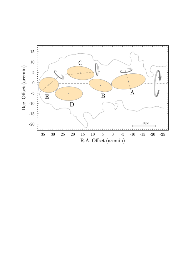
Figure 1: Morphology of a cometary-shaped cloud L1251 as revealed in Sato et al. 1994. The contour shows the integrated ¹³CO(1-0) emission at the lowest level of 1.5 K km s^-1 (Fig. 2b in Sato et al. 1994). Five ellipses represent locations and angular sizes of five C¹⁸O dense cores (Tables 1 and 2 in S94). The rotation of the individual cores is shown by small-sized gray arc arrows. The global rotation of the ¹³CO cloud is indicated by the large-sized arc arrow. For each arc arrow, denser gray color indicates the outer near side of the surface of the arc. The dashed lines are the rotation axes. The (0,0) map position is R.A. = 22:31:02.3, Dec = 75:13:39 (J2000). The adopted distance to the cloud is 300 pc.

Figure 1 shows schematically cloud morphology with ellipses representing locations and angular sizes of the five C¹⁸O dense cores. The boundary of the cloud (shown by a gray line) is set by the integrated ¹³CO(1-0) emission at the lowest level of 1.5 K km s^-1 (see Fig. 2b in S94). The (0,0) map position is R.A. = 22:31:02.3, Dec = 75:13:39 (J2000), which is fixed throughout the present paper.

The kinematic structure of the radial velocity field of L1251 reveals a number of peculiar features. The ¹³CO(1-0) and C¹⁸O(1-0) emission lines show a highly ordered velocity gradient of ${\cal G}\approx-0.5$ km s^-1 pc^-1  in the direction parallel to the minor axis of the cloud in the head of the cloud east of the offset R.A. $\sim 0^{\prime}$ in Fig. 1. Since it is interpreted as a solid body rotation, this gradient corresponds to an angular velocity of $\Omega_{\scriptscriptstyle{\rm CO}}\approx-2\times 10^{-14}$ rad s^-1. The negative sign means that the radial velocity is more negative to the north; i.e., the velocity gradient is directed N$\to$S across the head. This global motion is indicated in Fig. 1 by a large-sized arc arrow around the horizontal E–W axis (dashed line). In this respect L1251 resembles rotating elephant trunks found in star formation regions (Pound et al. 2003; Hily-Blant et al. 2005; Gahm et al. 2006). The cores A, B, and E disposed along this axis have approximately the same radial velocity $V_{\scriptscriptstyle\rm LSR}$$\approx-4.0$ km s^-1, whereas for the northern core C and the southern core D $V_{\scriptscriptstyle\rm LSR}$(C) $\approx-4.6$ km s^-1, and $V_{\scriptscriptstyle\rm LSR}$(D) $\approx-3.8$ km s^-1. (A typical uncertainty of $V_{\scriptscriptstyle\rm LSR}$ is $\sim 0.1$ km s^-1, S94.)

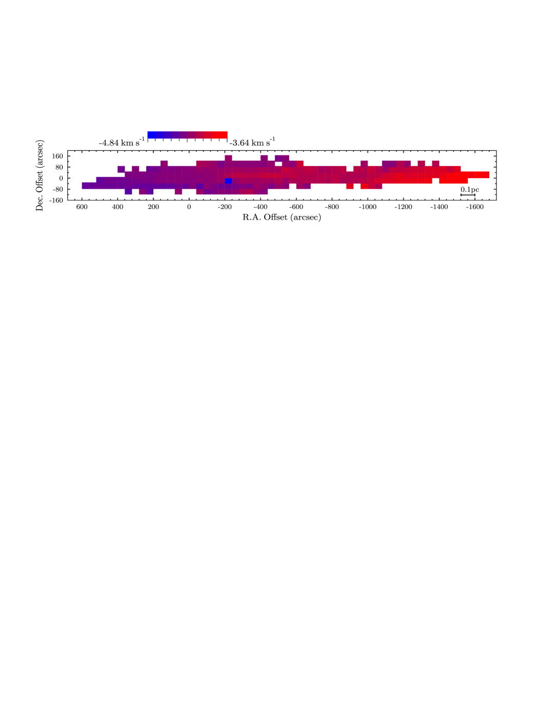
Figure 6: Same as Fig. 4 but for the NH₃(1,1) radial velocity field ($V_{\scriptscriptstyle\rm LSR}$).

However, observations in NH₃(1,1) revealed that despite the N$\to$S global velocity gradient, the northern core C exhibits a counter-rotation characterized by a highly ordered velocity gradient with ${\cal G}_{\rm C}\approx 1.7$ km s^-1 pc^-1, and position angle PA $\sim 30$° (E of N), corresponding to the angular velocity of $\Omega_{\scriptscriptstyle{\rm NH}_{3}}\approx 4\times 10^{-14}$ rad s^-1 (see Fig. 6 in Levshakov et al. 2014). Taking into account that C-bearing molecules are usually distributed in the outer parts of the cores (e.g., Tafalla et al. 2004), we conclude that the denser interior of this core traced by ammonia emission moves in a direction opposite to the global motion of the CO envelope.

For core A, Goodman et al.  (1993) reported an approximately east-west velocity gradient in NH₃ (${\cal G}_{\rm A}\approx 1.3$ km s^-1 pc^-1, and PA $\approx-77$°) with the rotation axis oriented almost perpendicular to the horizontal (E–W) rotation axis of the dark cloud L1251 (also Tóth & Walmsley 1996, hereafter TW96).

A more complex gas motion is observed in core E. According to Goodman et al.  (1993), who used spectral-line maps from Benson & Myers (1989), the velocity gradient direction in E is nearly orthogonal to the gradient direction in A (${\cal G}_{\rm E}\approx 3.5$ km s^-1 pc^-1, and PA $\approx-156$°). However, Caselli et al. (2002) mapped this core in N₂H⁺(1-0) with an angular resolution of 54″ (1.5 times the angular resolution of Benson & Myers) and found reverse velocity gradients in the eastern and western parts of the core suggestive of two counter-rotating adjacent clumps. For these clumps taken together, the N₂H⁺ tracer shows ${\cal G}_{\rm E}\approx 1.7$ km s^-1 pc^-1and PA $\approx-130$° (Caselli et al. 2002), meaning that the directions of increasing velocity for both NH₃ and N₂H⁺ are significantly correlated. Further single-dish and interferometric studies supported very complex kinematics, including rapid rotation, infall, and outflow motions in the dense core E (Lee et al. 2007). The directions of rotation and related rotation axes inferred from these studies are depicted in Fig. 1. No information exists on kinematic processes in cores B and D, except for radial velocities and linewidths of the ¹³CO(1-0) and C¹⁸O(1-0) lines measured in S94.

Here we continue our investigations of dense cores of the dark cloud L1251 in the NH₃(1,1) and (2,2) inversion transitions with the Effelsberg 100-m telescope. In a previous paper (Levshakov et al. 2014), we mapped core C. The present target is core A, which is one of the ammonia emitters exhibiting some of the narrowest ($\Delta v$ $\;\raise 1.29167pt\hbox{$<$\kern-7.5pt\raise-4.73611pt\hbox{$\sim$}}\;0.2$ km s^-1) lines ever observed (Jijina et al. 1999). For this reason L1251 was included in our list of targets used to validate the Einstein equivalence principle – local position invariance (Levshakov et al. 2010; Levshakov et al. 2013b).

2 Observations

The ammonia observations were carried out with the Effelsberg 100-m telescope in one session on April 22–27, 2014. The measurements were performed in the position-switching mode with the backend XFFTS (eXtended bandwidth FFTS) operating at 100 MHz bandwidth and providing 32,768 channels for each polarization. The resulting channel width was $\Delta_{\rm ch}=0.039$ km s^-1, but the true velocity resolution is 1.16 times coarser (Klein et al. 2012). The NH₃ lines were measured with a K-band high-electron mobility transistor (HEMT) dual channel receiver, yielding spectra with a spatial resolution of $40^{\prime\prime}$ (FWHP) in two orthogonally oriented linear polarizations at the rest frequency of the $(J,K)=(1,1)$ and (2,2) lines, $f_{1,1}=23694.495487$ MHz and $f_{2,2}=23722.633644$ MHz (Kukolich 1967). Averaging the emission from both channels, the typical system temperature (receiver noise and atmosphere) is 100 K on a main beam brightness temperature scale.

The mapping was done on a 40″ grid. The pointing was checked every hour by continuum cross scans of nearby continuum sources. The pointing accuracy was better than $5^{\prime\prime}$. The spectral line data were calibrated by means of continuum sources with a known flux density. We mainly used G29.96–0.02 (Churchwell et al. 1990). With this calibration source, a main beam brightness temperature scale, $T_{\scriptscriptstyle\rm MB}$, can be established. Since the main beam size ($40^{\prime\prime}$) is smaller than most core radii ($>50^{\prime\prime}$) of our target, the ammonia emission couples well to the main beam so that the $T_{\scriptscriptstyle\rm MB}$ scale is appropriate. Compensations for differences in elevation between the calibrator and the source were $\;\raise 1.29167pt\hbox{$<$\kern-7.5pt\raise-4.73611pt\hbox{$\sim$}}\;20$% and have not been taken into account. Similar uncertainties of the main beam brightness temperature were found from a comparison of spectra toward the same position taken on different dates.

The typical rms noise in our observations was 0.3 K per channel in main-beam brightness temperature units ($150^{\rm s}$ ON and $150^{\rm s}$ OFF positions for one scan). Some points were observed several times resulting in rms $\sim 0.15$ K. For a characteristic line width of 0.2 km s^-1 (see below), this yields typical rms values of 0.05 K km s^-1, so that we choose 0.2 K km s^-1 as the lowest contour in the following.

3 Results

The ammonia spectra were analyzed in the same way as in Levshakov et al. (2014). There are no features with two velocity components. The radial velocity, $V_{\scriptscriptstyle\rm LSR}$, the linewidth $\Delta v$, the optical depths $\tau_{\scriptscriptstyle\rm 11}$ and $\tau_{\scriptscriptstyle\rm 22}$, the integrated ammonia emission $\int$$T_{\scriptscriptstyle\rm MB}$$dv$, and the kinetic temperature $T_{\rm kin}$  are all well-determined physical parameters, whereas the excitation temperature $T_{\rm ex}$, the ammonia column density $N$(NH₃), and the gas density $n_{\scriptscriptstyle{\rm H}_{2}}$ are less certain since they depend on the beam filling factor $\eta$, which is not known for unresolved clumps. Assuming that $\eta$ ranges between $\eta_{\rm min}$ and 1, one can estimate limits for $T_{\rm ex}$, $N$(NH₃), and $n_{\scriptscriptstyle{\rm H}_{2}}$, where a minimum value of $n_{\scriptscriptstyle{\rm H}_{2}}$ is obtained by the choice of $\eta=1$. The corresponding equations are given in Appendix A in Levshakov et al. (2013a, hereafter L13).

The errors of the model parameters were estimated from the diagonal elements of the covariance matrix calculated for the minimum of $\chi^{2}$. The error in $V_{\scriptscriptstyle\rm LSR}$ was also estimated independently by the $\Delta\chi^{2}$ method (Press et al. 1992). When the two estimates differed, the larger error was adopted. Table 1 illustrates that a typical uncertainty of $V_{\scriptscriptstyle\rm LSR}$ and $\Delta v$ at peak intensities of NH₃(1,1) is $\sim 0.01$ km s^-1 ($1\sigma$ confidence level, C.L.). Below we describe the obtained results in detail.

3.1 Global gas morphology from NH₃

Our NH₃ observations cover the whole molecular core A and part of core B of L1251 and consist of 300 measured positions, each of which is represented by a color box in the NH₃(1,1) integrated intensity map in Fig. 2a. The NH₃ map clearly reveals three peaks that are labeled by $\alpha$, $\beta$, and $\gamma$. Their parameters are given in Table 1. In Fig. 2a, the peak positions of cores B and A have offsets $(\Delta\alpha,\Delta\delta)=(362\arcsec,-76\arcsec)$ and $(-474\arcsec,38\arcsec)$, respectively. Thus, the ammonia $\beta$ peak coincides with the C¹⁸O peak A, whereas the C¹⁸O peak B is slightly shifted from the ammonia $\alpha$ peak to the southeast. For this reason we will call the whole structure traced by NH₃ emission as L1251A.

As mentioned above, the ammonia map was sampled at intervals of 40″, which is half the grid size of 80″ in TW96. The denser sampling resulted in a different apparent morphology of the NH₃ distribution. For instance, TW96 identified four ammonia cores dubbed as “T1” to “T4” in decreasing R.A. direction. The first three T1–T3 have a common envelope, whereas T4 is separated (see Fig. 2b). However, our results show that these two zones of ammonia emission are not separated, but, in fact, all four cores belong to a central part of a continuous elongated structure that is much larger than the area of the NH₃ emission mapped by TW96. The peak positions of cores T1-T4 are marked by black stars in Fig. 2b for comparison with our observations. The known infrared sources are indicated as well.

The shape of the filament at the lowest level of 0.2 K km s^-1 can be approximated by an ellipse with the angular sizes of the major (E-W) and minor (S-N) axes on the plane of the sky of about 38′ and 3′. The projected linear sizes of these axes are $\ell_{1}\approx 3.3$ pc and $\ell_{2}\approx 0.3$ pc; i.e., the aspect ratio is $\varepsilon\approx 11$.

The NH₃(1,1) integrated intensities $I(\Delta\alpha,\Delta\delta)=\int T_{\rm MB}dv$ form three condensations around the $\alpha$, $\beta$, and $\gamma$ peaks, which are clearly seen in Fig. 2c where we plot the sum over $\Delta\delta$ values, $\sum_{\Delta\delta}I_{\Delta\alpha}(\Delta\delta)$, at each fixed $\Delta\alpha$ as a function of R.A. The shape of this function, shown by gray in Fig. 2c, allows us to formally assign the boundaries for these condensations: $-160\arcsec\;\raise 1.29167pt\hbox{$<$\kern-7.5pt\raise-4.73611pt\hbox{$\sim$}}\;\Delta\alpha\leq 600\arcsec$ for $\alpha$, $-880\arcsec\;\raise 1.29167pt\hbox{$<$\kern-7.5pt\raise-4.73611pt\hbox{$\sim$}}\;\Delta\alpha\;\raise 1.29167pt\hbox{$<$\kern-7.5pt\raise-4.73611pt\hbox{$\sim$}}\;-160\arcsec$ for $\beta$, and $-1640\arcsec\leq\Delta\alpha\;\raise 1.29167pt\hbox{$<$\kern-7.5pt\raise-4.73611pt\hbox{$\sim$}}\;-880\arcsec$ for $\gamma$.

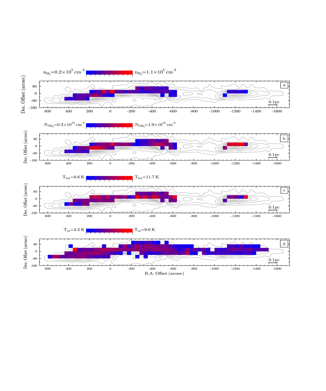
Figure 3: Distributions of the measured parameters in L1251A: (a) — the gas volume density, $n_{\scriptscriptstyle{\rm H_{2}}}$; (b) the NH₃ column density, $N_{\scriptscriptstyle{\rm NH_{3}}}$; (c) the kinetic temperature, $T_{\rm kin}$; and (d) the excitation temperature, $T_{\rm ex}$. Three parameters $n_{\scriptscriptstyle{\rm H_{2}}}$, $N_{\scriptscriptstyle{\rm NH_{3}}}$, and $T_{\rm kin}$ were measured at the 54 positions where both the NH₃(1,1) and (2,2) lines were observed, whereas $T_{\rm ex}$ was estimated from the NH₃(1,1) lines, which are not very weak. Each color box has a size of $40^{\prime\prime}\times 40^{\prime\prime}$ and its bottom left corner corresponds to the telescope pointing. The contours are the NH₃(1,1) integrated intensity map. The starting point for the contour levels is 0.2 K km s^-1; the increment is 1.0 K km s^-1. The (0,0) map position is as in Fig. 1. We note that for the beam filling factor $\eta<1$, certain parameters could be larger (see Sect. 3 and 3.1 for details).

The thickness of the filament along the line of sight (the third axis $\ell_{3}$) can be estimated from the measured ammonia column density, $N_{\scriptscriptstyle\rm NH_{3}}$, and the gas number density, $n_{\scriptscriptstyle\rm H_{2}}$, assuming a mean abundance ratio $[{\rm NH}_{3}]/[{\rm H}_{2}]=(4.6\pm 0.3)\times 10^{-8}$ found in dark clouds (Dunham et al. 2011). The measured values of $n_{\scriptscriptstyle\rm H_{2}}$ and $N_{\scriptscriptstyle\rm NH_{3}}$ over the ammonia map are shown in panels (a) and (b) in Fig. 3. Along the major axis $\ell_{1}$, we observed both the NH₃(1,1) and (2,2) transitions at 54 positions between the offsets $\Delta\alpha=440\arcsec$ and $-1280\arcsec$, except for a gap $-1040\arcsec\leq\Delta\alpha\leq-640\arcsec$. Averaging this dataset we obtain ${\langle N\rangle}_{\scriptscriptstyle\rm NH_{3}}=(1.03\pm 0.05)\times 10^{15}$ cm^-2 ($1\sigma$ C.L.) and ${\langle n\rangle}_{\scriptscriptstyle\rm H_{2}}=(3.9\pm 1.3)\times 10^{4}$ cm^-3 under the assumption that the beam filling factor $\eta=1$ (Eqs. (A.19) and (A.21) in L13); i.e., we observe a rather small ($\sim 5\%$) fluctuation in column densities along with a significant variation ($\;\raise 1.29167pt\hbox{$>$\kern-7.5pt\raise-4.73611pt\hbox{$\sim$}}\;30\%$) in gas number densities. For instance, a twofold variation is found between $\alpha$ peak where $n^{\scriptscriptstyle\alpha}_{\scriptscriptstyle{\rm H_{2}}}=7.1\times 10^{4}$ cm^-3 and other peaks with $n^{\scriptscriptstyle\beta}_{\scriptscriptstyle{\rm H_{2}}}=3.8\times 10^{4}$ cm^-3 and $n^{\scriptscriptstyle\gamma}_{\scriptscriptstyle{\rm H_{2}}}=3.3\times 10^{4}$ cm^-3. Besides this, a sharp change in $n_{\scriptscriptstyle{\rm H_{2}}}$ is measured between the offsets (0″,0″) and $(0\arcsec,-40\arcsec)$ showing $n_{\scriptscriptstyle{\rm H_{2}}}=6.8\times 10^{4}$ cm^-3 and $1.7\times 10^{4}$ cm^-3, respectively.

The reason for such a high density fluctuation is not clear. It might be due to the used filling factor $\eta=1$ and the presence of small clumps with linear sizes less than 0.05 pc that are unresolved in our observations. Shown in Fig. 3d, the excitation temperature $T_{\rm ex}$, also estimated at $\eta=1$ (Eq. (A.10) in L13), may be inaccurate as well, since $T_{\rm ex}$ then corresponds to a minimum value. With increasing $T_{\rm ex}$ (i.e., decreasing $\eta$) and, as a result, decreasing difference $(T_{\rm kin}-T_{\rm ex})$, the estimate of $n_{\scriptscriptstyle{\rm H_{2}}}$ loses stability (Ho & Townes 1983). In this difference, $T_{\rm kin}$ is actually a fixed quantity since the kinetic temperature is found to be almost constant over the whole filament (see Fig. 3c). Its mean value is $\langle T_{\rm kin}\rangle=10.12\pm 0.08$ K.

For the mean abundance $[{\rm NH}_{3}]/[{\rm H}_{2}]=4.6\times 10^{-8}$, the ratio of ${\langle N\rangle}_{\scriptscriptstyle\rm NH_{3}}$ and ${\langle n\rangle}_{\scriptscriptstyle\rm H_{2}}$ gives the mean thickness of the filament of $\langle{\ell}_{3}\rangle\sim 0.2$ pc, which is comparable to $\ell_{2}$. We note that for $\eta<1$, $\langle{\ell}_{3}\rangle$ would become smaller. Thus, if we use the sample means, then the filamentary structure traced by ammonia emission resembles a prolate ellipsoid of revolution (rod-like) with $\ell_{1}\gg\ell_{2}\;\raise 1.29167pt\hbox{$>$\kern-7.5pt\raise-4.73611pt\hbox{$\sim$}}\;\ell_{3}$.

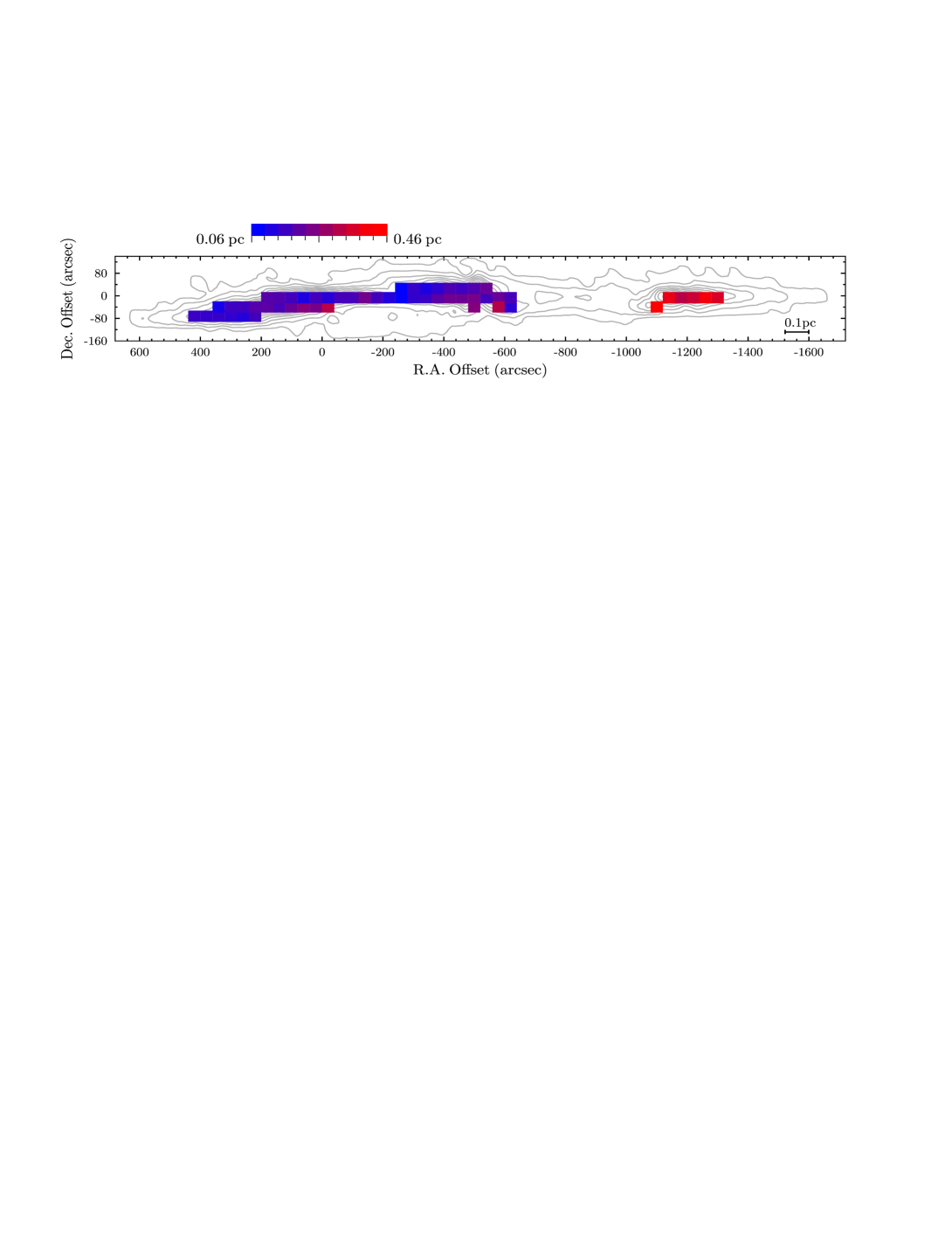
Figure 4: Thickness along the line of sight through the core L1251A estimated from the measured column densities $N_{\scriptscriptstyle{\rm NH_{3}}}$ and number densities $n_{\scriptscriptstyle{\rm H_{2}}}$ shown in Fig. 3. The mean abundance ratio of $[{\rm NH}_{3}]/[{\rm H}_{2}]=4.6\times 10^{-8}$ (Dunham et al. 2011) is fixed for the whole filament. The (0,0) map position is as in Fig. 1. We note that for the beam filling factor $\eta<1$, the thickness is smaller (see Sects. 3 and 3.1 for details).

However, the ammonia filament may have a more complex morphology if one compares individual gas densities at each point. Following this approach, we obtained local thickness at different positions as displayed in Fig. 4. It is seen that the linear dimension $\ell_{3}$ within the area occupied by the $\alpha$ and $\beta$ condensations is $\sim 0.2$ pc, whereas it is two times larger, $\sim 0.4$ pc, at the position of the $\gamma$ condensation.

It has to be noted that such calculations of $\ell_{3}$ are only legitimate at gas densities below or near the critical density, $n_{\scriptscriptstyle{\rm H_{2}}}\leq n_{\rm cr}$, since otherwise the observed line intensity is no longer unambiguously related to the gas density because the collisionally induced transitions produce no photons. For NH₃(1,1), the critical density at $T_{\rm kin}$ = 10 K is $n_{\rm cr}=3.90\times 10^{3}$ cm^-3 (Maret et al. 2009), which is an order of magnitude lower than the measured mean value of ${\langle n}\rangle_{\scriptscriptstyle{\rm H_{2}}}$. Therefore, the estimates of $\ell_{3}$ must be taken with some caution. Nevertheless, a sheet-like geometry of L1251A with $\ell_{3}\sim\ell_{1}$ may be excluded since it would produce too low a gas number density, $n_{\scriptscriptstyle{\rm H_{2}}}\sim 2\times 10^{3}$ cm^-3 — an order of magnitude lower than the measured values of $n_{\scriptscriptstyle{\rm H}_{2}}$. An $\eta<1$ would make $\ell_{3}$ even shorter.

In what follows, we assume that the filament has a rod-like geometry consisting of two cylinders with different cross-sections: a circular one with diameter 0.2 pc for $\alpha$ and $\beta$, and an elliptical cylinder with the major and minor axes of 0.4 pc and 0.2 pc for $\gamma$. Their corresponding linear sizes are 2.2 pc and 1.1 pc. The mean gas number densities are ${\langle n\rangle}_{\alpha\beta}=(4\pm 2)\times 10^{4}$ cm^-3 (sample size = 48), and ${\langle n\rangle}_{\gamma}=(2.6\pm 0.4)\times 10^{4}$ cm^-3 (sample size = 6).

It is interesting to compare our results with previous ones. According to TW96, the angular size (E-W) of the combined cores T1–T3 is $\sim 7\arcmin$, which is in line with the ammonia map of Goodman et al. (1993). Together with T4, the total size of the T1–T4 complex in the E-W direction is about 15′, which is more than two times shorter as compared with $\ell_{1}$. In the orthogonal direction (S-N), we observe the same extension of the ammonia map as reported by Goodman et al. and TW96.

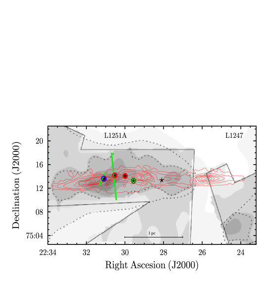
Figure 5: Portion of Fig. 17 from Kirk et al. (2009) with extended structure toward L1251A and L1247. The gray scale shows the distribution of visual extinction as derived from the Digitized Sky Survey (Dobashi et al. 2005), and the superimposed higher resolution extinction maps (outlined by solid straight black lines) observed with the Spitzer Infrared Array Camera (IRAC; 3.6-8.0 $\mu$m) and Multiband Imaging Photometer (MIPS; 24-160 $\mu$m). Two dashed lines refer to Dobashi $A_{V}=1$ mag and Spitzer $A_{V}=5$ mag. The colored markers show the location and spectral type of the young stellar object (YSO) candidates: red/green/blue for Class I/Flat/Class II. The black stars are the same markers as in Fig. 2b. The NH₃(1,1) integrated intensity map, as in Fig. 4, is denoted by the red contours. The approximate orientation and linear size of a jet extending about 10′ and a small bipolar nebula to the east of the jet (solid green lines) are copied from Fig. 1 in Lee et al. (2010).

The previous ammonia observations did not reveal the $\gamma$ condensation which is partly overlapping the nearby dark cloud L1247 (Fig. 5). The maximum of the NH₃(1,1) integrated intensity lies in the region with minimum visual extinction just between L1251A and L1247. Thus, approximately three fourths of the ammonia map coincides with the most prominent filament evident in the dust emission (dark gray area with $A_{V}\;\raise 1.29167pt\hbox{$>$\kern-7.5pt\raise-4.73611pt\hbox{$\sim$}}\;5$ mag in Fig. 5), whereas one fourth follows a weaker dust emission with $A_{V}\sim 1$ mag.

The question then arises as to how it is possible that in the $\gamma$ region the maximum of the ammonia emission originates in areas with minimal visual extinction. This is perhaps due to small scale clumping with the NH₃ gas providing high visual extinction but not covering the entire area, hinting at an $\eta<1$ for this region. Possibly, $\eta$ is smaller in the $\gamma$ fragment than in $\alpha\beta$. In Sect. 3.3, we discuss that the average H₂ density is well below what is deduced from NH₃. This is also consistent with small scale clumping.

The comparison with the C¹⁸O(1-0) map, which has the major (E$\to$W) and minor (S$\to$N) axes of 17′ $\times$ 7′ (Fig. 2 in S94), shows that in general both NH₃ and C¹⁸O trace each other, but the former is more concentrated on the horizontal E–W axis. This is not surprising since the C¹⁸O(1-0) transition becomes excited at densities an order of magnitude lower than needed for NH₃(1,1). However, an unexpected result is that a rather large area of ammonia emission from the western part of L1251A ($\gamma$ condensation in Fig. 2a) is not seen in C¹⁸O: this part of L1251 was mapped only in ¹³CO(1-0) (Fig. 1) and in dust emission (Fig. 5). The ¹³CO “tail” of L1251 west of the offset R.A. $\sim 0^{\prime}$ in Fig. 1 has an angular size of $\sim 27\arcmin\times 20\arcmin$, which is much larger than regions with visual extinction $A_{V}\sim 5$ mag and the similarly extended C¹⁸O emission.

Considering the spatial distributions of these emitters, we see that the tail of L1251A has a cocoon-like morphology with radial stratification from the outer to the innermost layers seen in ¹³CO, C¹⁸O, dust emission, and NH₃. The radius of the first region projected on the plane of the sky is $R_{1}\sim 0.9$ pc (¹³CO), the second $R_{2}\sim 0.3$ pc (C¹⁸O and dust), and the third $R_{3}\sim 0.13$ pc (NH₃). The ambient medium traced by ¹²CO emission (the outermost envelope) has a very large angular size and irregular morphology as displayed in Fig. 1 in Grenier et al. (1989).

In the next section, we show that all three ammonia condensations $\alpha$, $\beta$, and $\gamma$ are involved in a common global motion of the filamentary structure with some intrinsic peculiarities.

3.2 Global gas kinematics from NH₃

The NH₃ radial velocity map is shown in Fig. 6. In our analysis of ammonia spectra, all hyperfine structure (hfs) components of the NH₃(1,1) and (2,2) transitions were fitted simultaneously to determine the total optical depth, $\tau_{\rm tot}$, in the respective inversion transition, the LSR velocity of the line, $V_{\scriptscriptstyle\rm LSR}$, the intrinsic full-width at half power linewidth, $\Delta v$ (FWHP), for individual hf components, and the amplitude, ${\cal A}$ (see Appendix A in L13). For unsaturated lines ($\tau_{\rm hf}\;\raise 1.29167pt\hbox{$<$\kern-7.5pt\raise-4.73611pt\hbox{$\sim$}}\;1$), the velocity $V_{\scriptscriptstyle\rm LSR}$ represents an intensity-weighted average centroid velocity along the line of sight through the cloud.

If the cloud rotates as a solid body, $V_{\scriptscriptstyle\rm LSR}$ is independent of distance along the line of sight, and linearly dependent on the coordinates in the plane of the sky (e.g., Goodman et al. 1993; Belloche 2013). Then, the cloud rotation velocity field is defined by the equation

$${\@vec{V}}=\@vec{\Omega}\times{\@vec{R}}\ ,$$ (1)

where $\Omega$ is the angular velocity, and $R$ the distance to the rotation axis. This means that a cloud in solid-body rotation should demonstrate a linear gradient, $\nabla$$V_{\scriptscriptstyle\rm LSR}$, across the surface of a map, orthogonal to the rotation axis $\@vec{\Omega}$. This is just the case of L1251A where the velocity gradient in the direction E$\to$W along the major axis can be easily identified by eye (Fig. 6).

3.2.1 The whole filament, $-1640\arcsec\leq\Delta\alpha\leq 600\arcsec$

The $V_{\scriptscriptstyle\rm LSR}$ values are systematically increasing with decreasing R.A. (E$\rightarrow$W) on the total linear scale of the filament $\ell_{1}\approx 3.3$ pc. As it follows from Fig. 6, the velocity difference between the eastern and western edges of the filament is $\Delta V\approx 0.7$ km s^-1, meaning that the gradient becomes $\nabla$$V_{\scriptscriptstyle\rm LSR}$$\approx 0.2$ km s^-1 pc^-1.

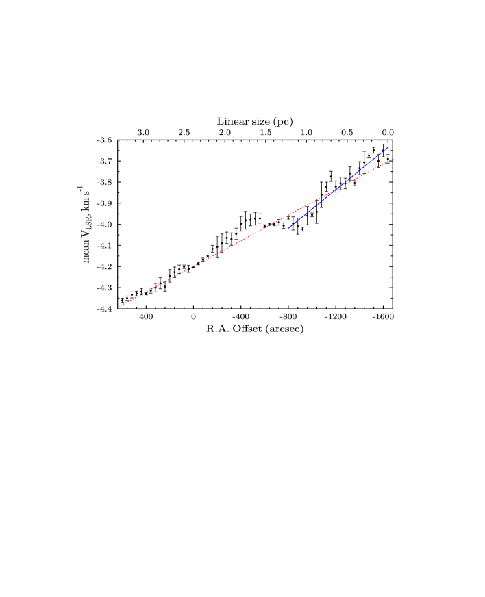
Figure 7: Position-velocity diagram of NH₃(1,1) along the direction of the velocity gradient (E $\to$ W). At each offset $\Delta\alpha$, the measured centroid velocities ($V_{\scriptscriptstyle\rm LSR}$) are averaged across the filament in the direction S$\to$N. The error bars (the standard deviation of the mean) result from this averaging. The different positions were weighted inversely proportional to the variance. The linear regression for the total range is shown by red: $V_{0}=-4.199(1)-0.000303(3)\Delta\alpha$ (km s^-1) (here $\Delta\alpha$ is in arcsec). For the $\alpha\beta$ condensation $(-480\arcsec\leq\Delta\alpha\leq 600\arcsec)$, the regression line is practically the same. For the $\gamma$ condensation $(-1640\arcsec\leq\Delta\alpha\leq-800\arcsec)$, it is shown by a blue line with $V_{0}=-4.38(1)-0.00046(1)\Delta\alpha$ (km s^-1). The number in parentheses is the one-sigma ($1\sigma$) uncertainty in the last digit of the given value. The (0,0) map position is as in Fig. 1.

The same gradient can be found from the regression analysis shown in Fig. 7, where a functional dependence of spatial averages of $\langle$$V_{\scriptscriptstyle\rm LSR}$$\rangle$ on R.A. is depicted. At each offset $\Delta\alpha$, the weighted mean value of $\langle$$V_{\scriptscriptstyle\rm LSR}$$\rangle$ was found from averaging along the S$\to$N direction with weights inversely proportional to the uncertainties of the measured line-of-sight velocities. The regression line (shown by red) is defined by

$$V_{0}=-4.199(1)-0.000303(3)\Delta\alpha\ ({\rm km\leavevmode\nobreak\ s}^{-1})\ ,$$ (2)

which corresponds to $\nabla$$V_{\scriptscriptstyle\rm LSR}$$=0.208\pm 0.003$ km s^-1 pc^-1. Here, the numbers in parentheses are $1\sigma$ errors on the last digit, and $\Delta\alpha$ is counted in arcsec.

It follows from Eqs. (1) and (2) that the angular velocity of the whole filament around the vertical axis (S$\to$N) is $\Omega^{\scriptscriptstyle\rm SN}_{\rm tot}\approx 7.0\times 10^{-15}$ rad s^-1, and the period for a complete rotation $t^{\scriptscriptstyle\rm SN}_{\rm tot}\approx 3\times 10^{7}$ yr.

3.2.2 The $\alpha$ and $\beta$ kinematic fragments, $-480\arcsec\leq\Delta\alpha\leq 600\arcsec$

Figure 7 demonstrates that radial velocities increase gradually with R.A. over the area occupied by the $\alpha$ and $\beta$ condensations from the offset $\Delta\alpha=600\arcsec$ to $\Delta\alpha\sim-480\arcsec$. The regression line for this kinematic fragment is practically the same as for the whole filament:

$$V_{0}=-4.197(2)-0.000305(7)\Delta\alpha\ ({\rm km\leavevmode\nobreak\ s}^{-1})\ .$$ (3)

Its angular velocity around the vertical axis (S$\to$N) is $\Omega^{\scriptscriptstyle\rm SN}_{\alpha\beta}\simeq\Omega^{\scriptscriptstyle\rm SN}_{\rm tot}$.

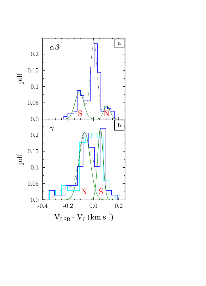
Figure 8: Histograms are the probability density functions (pdfs) of line centroid velocity fluctuations $\Delta V=V_{\scriptscriptstyle\rm LSR}-V_{0}$, and the smooth curves are their approximations by Gaussians. Here $V_{0}$ is the systemic velocity component defined by the regression lines shown in Fig. 7. Panels (a) and (b) represent the $\alpha\beta$ (red regression line in Fig. 7) and $\gamma$ (blue regression line in Fig. 7) condensations. The lateral peaks labeled by the letters “N” and “S” correspond to the northern and southern ridges of the filament. Note the opposite chirality of the angular rotation around the horizontal axis E$\to$W (see Sects. 3.2.2 and 3.2.4 for details).

It is noteworthy that the gas in this area exhibits an additional spinning around the horizontal axis (E$\to$W), which is revealed in a systematic difference between the radial velocities toward the northern and southern ridges of the filament. To specify this effect numerically, we considered the probability density function (pdf) of line centroid velocity fluctuations $\Delta V=V_{\scriptscriptstyle\rm LSR}-V_{0}$ calculated at each offset position on the map of the $\alpha\beta$ fragment. Here, $V_{0}$ is a local systemic velocity at a given $\Delta\alpha$, which is defined by (3). The obtained pdf is shown by the blue histogram (approximated by a Gaussian) in Fig 8a. It consists of three peaks: the central component with $\Delta V=0$ km s^-1, and the two lateral components with $\Delta V_{\scriptscriptstyle\rm N,S}\approx\pm 0.11$ km s^-1. In this case, the positive northern component $\Delta V_{\scriptscriptstyle\rm N}$ indicates that the line-of-sight velocity is higher to the north, whereas the negative southern component $\Delta V_{\scriptscriptstyle\rm S}$ shows that $V_{\scriptscriptstyle\rm LSR}$ is predominantly directed to the observer.

The velocity difference between these two filament ridges is $\sim 0.22$ km s^-1, which gives the gradient $\nabla$$V_{\scriptscriptstyle\rm LSR}$$\sim 0.7$ km s^-1 pc^-1 in the direction S$\to$N. The corresponding angular velocity $\Omega^{\scriptscriptstyle\rm EW}_{\alpha\beta}$ has the opposite sign to the rotation of the CO envelope ($\Omega_{\scriptscriptstyle{\rm CO}}\approx-2\times 10^{-14}$ rad s^-1) and equals $\Omega^{\scriptscriptstyle\rm EW}_{\alpha\beta}\approx 2\times 10^{-14}$ rad s^-1 ($t^{\scriptscriptstyle\rm EW}_{\alpha\beta}\approx 1\times 10^{7}$ yr).

3.2.3 The bar, $-800\arcsec\leq\Delta\alpha\leq-480\arcsec$

Figure 7 shows that near the geometric center of the filament in the range $-800\arcsec\leq\Delta\alpha\leq-480\arcsec$, the mean radial velocity between the adjoining points is held constant: $\langle V_{\scriptscriptstyle\rm LSR}\rangle=-3.997\pm 0.004$ km s^-1. This kinematic fragment is also characterized by an extremely low linewidth of ammonia lines, $\Delta v$ $\sim 0.1-0.2$ km s^-1 (blue and red filled circles in Fig. 2b), and decreasing gas density $n_{\scriptscriptstyle{\rm H_{2}}}$ from $4\times 10^{4}$ cm^-3 to $2\times 10^{4}$ cm^-3 with changing $\Delta\alpha$ from $-480\arcsec$ to $-600\arcsec$ along the cut $\Delta\delta=0\arcsec$. Beyond this interval, between $\Delta\alpha=-640\arcsec$ and $-1040\arcsec$, we did not detect the second ammonia transition NH₃(2,2), and, therefore, the gas number density was not estimated. The same tendency is observed for the ammonia column density: $N$(NH₃) decreases from $1.5\times 10^{15}$ cm^-2 to $0.5\times 10^{15}$ cm^-2 within the interval $-600\arcsec\leq\Delta\alpha\leq-480\arcsec$.

In what follows, we refer to this fragment of the filament as a “bar”. Figure 2a shows that it starts at the western edge of the $\beta$ condensation and its projected linear size is $\ell_{\rm bar}\approx 0.5$ pc.

3.2.4 The $\gamma$ kinematic fragment, $-1640\arcsec\leq\Delta\alpha\leq-800\arcsec$

The regression line of the $\gamma$ kinematic fragment, ranging from $\Delta\alpha=-800\arcsec$ to $-1640\arcsec$ (shown by blue in Fig. 7), is defined by

$$V_{0}=-4.38(1)-0.00046(1)\Delta\alpha\ ({\rm km\leavevmode\nobreak\ s}^{-1})\ ,$$ (4)

i.e., $\nabla$$V_{\scriptscriptstyle\rm LSR}$$=0.316\pm 0.007$ km s^-1 pc^-1. Thus, the western part of the filament rotates around the vertical axis (S$\to$N) with a slightly higher angular velocity $\Omega^{\scriptscriptstyle\rm SN}_{\gamma}\approx 1.0\times 10^{-14}$ rad s^-1 than $\Omega^{\scriptscriptstyle\rm SN}_{\rm tot}$.

Toward the $\gamma$ condensation, we also reveal an additional systemic motion around the axis E$\to$W: the radial velocity is more negative to the north than what is observed from the global rotation of the CO envelope. Applying the same procedure as for the $\alpha\beta$ fragment, we calculated pdfs of the residuals $\Delta V$ using the two definitions of the systemic velocity $V_{0}$ given by Eqs. (2) and (4). The resulting distribution functions are shown by the cyan and blue histograms in Fig. 8b, respectively. It is seen that the definition (2) based on the total dataset provides unresolved lateral peaks and a broad central component, whereas the regression line (4) allows us to partly resolve the lateral peaks.

It is remarkable that in this case we observe spinning with opposite chirality (dextral vs sinistral): the northern peak is shifted to negative line-of-sight velocities, and the southern — to positive velocities. Because of an asymmetric shape of the northern peak, it was approximated by a convolution of two Gaussians shown by the dotted curve in Fig. 8b. Their barycenter is $\Delta V_{\scriptscriptstyle\rm N}\approx-0.089$ km s^-1, whereas the center of the southern component is $\Delta V_{\scriptscriptstyle\rm S}\approx 0.056$ km s^-1. This leads to a velocity difference between the northern and southern ridges of the filament of $\sim-0.15$ km s^-1and a gradient $\nabla$$V_{\scriptscriptstyle\rm LSR}$$\sim-0.5$ km s^-1 pc^-1. The corresponding angular velocity of the $\gamma$ fragment around the axis E$\to$W is $\Omega^{\scriptscriptstyle\rm EW}_{\gamma}\approx-2\times 10^{-14}$ rad s^-1 ($t^{\scriptscriptstyle\rm EW}_{\gamma}\approx 1\times 10^{7}$ yr).

Thus, here we find two kinematic fragments of opposite chirality when the filament is viewed from the eastern footpoint along the axis E$\to$W: the fragment $\gamma$ spins clockwise, whereas the fragment $\alpha\beta$ rotates counterclockwise. The filament chirality directly indicates the magnetic field helicity of two types, negative and positive (e.g., Martin 1998).

It should be emphasized that all measured periods exceed the age of the supernova remnant considerably, $t_{\scriptscriptstyle\rm SNR}\sim 4\times 10^{4}$ yr, mentioned in Sect. 1. Since dark clouds evolve slowly, this may imply that the dynamical stage of L1251A was triggered by another supernova exploded in the past $10^{6-7}$ yr in this region, as suggested in S94. A similar lifetime of $\sim 10^{6}$ yr for starless cores with average volume density $n\sim 10^{4}$ cm^-3 was estimated by Lee & Myers (1999), among others.

3.2.5 Smoothness of the velocity field

The distribution of the centroid velocities over the map of the filament (Fig. 6) reveals only one offset position $(\Delta\alpha,\Delta\delta)=(-200\arcsec,-40\arcsec)$ (blue square) with a peculiar velocity $V_{\scriptscriptstyle\rm LSR}$ = $-4.84(3)$ km s^-1 which deviates noticeably from velocities measured at the neighboring positions. For instance, $V_{\scriptscriptstyle\rm LSR}$$(-200\arcsec,-80\arcsec)=-4.32(3)$ km s^-1, $V_{\scriptscriptstyle\rm LSR}$$(-200\arcsec,0\arcsec)=-4.019(7)$ km s^-1, or $V_{\scriptscriptstyle\rm LSR}$$(-240\arcsec,0\arcsec)=-3.961(7)$ km s^-1, which gives a break of $|\Delta V|\sim 0.5-0.9$ km s^-1 on a scale $\sim 0.05$ pc. The nature of the outlier at ($-200$″,$-40$″) is not clear and requires further exploration. We note that this peculiar velocity is not a product of measurement errors but is connected with other peculiarities outlined further below in the same section.

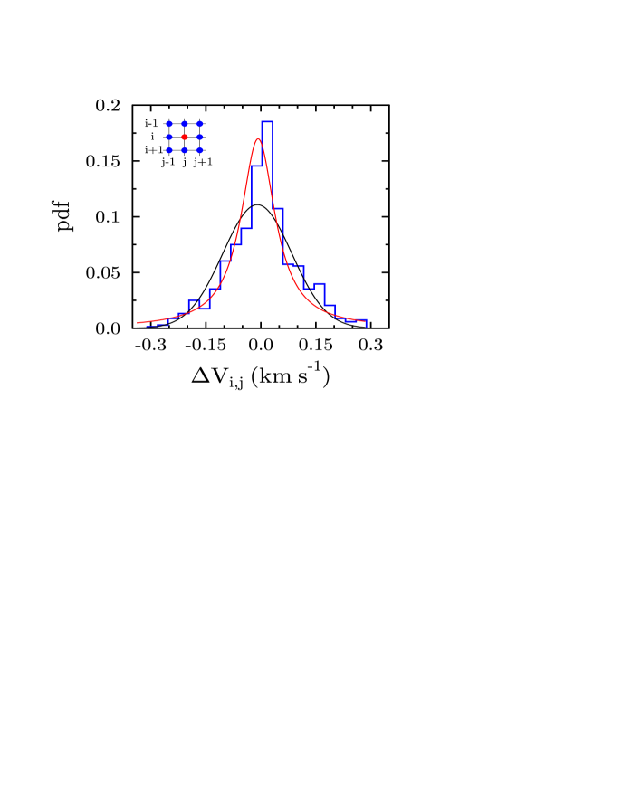
Figure 9: Histogram is the probability density function (pdf) of line centroid velocity fluctuations between neighboring positions over the whole NH₃ map of the filament L1251A except for the outlier at the offset $(\Delta\alpha,\Delta\delta)=(-200$″,$-40$″). In the upper left hand corner, the grid with color points illustrates the calculation of $\Delta V_{i,j}$: for a current position $(i,j)$ (marked by red), the velocity differences are calculated between each blue point and the central red point. The total number of different pairs is 680. The histogram is approximated by a Gauss (black) and a Lorentz (red) function with the widths (FWHP) of $\Delta v_{\scriptscriptstyle\rm G}=0.22$ km s^-1 and $\Delta v_{\scriptscriptstyle\rm L}=0.11$ km s^-1.

At all other offsets, $V_{\scriptscriptstyle\rm LSR}$ changes smoothly from point to point. The variance of centroid velocity fluctuations at a given spatial lag can be estimated from velocity differences between neighboring positions. The histogram in Fig. 9 shows the pdf of such differences at the lags $40\arcsec$ and $\sqrt{2}\cdot 40\arcsec$ for the whole filament L1251A except for the outlier at the offset ($-200$″,$-40$″). For a given position $i,j$ (shown by red on the grid in the top lefthand corner of Fig. 9), the velocity differences $\Delta V_{i,j}$ are calculated between each blue point on the grid and the central red point. The total sample size consists of $p=680$ pairs of these neighboring points. The velocity difference pdf was approximated by Gauss (black curve) and Lorentz (red curve) functions with the widths (FWHP) of $\Delta v_{\scriptscriptstyle\rm G}\approx 0.22$ km s^-1 and $\Delta v_{\scriptscriptstyle\rm L}\approx 0.11$ km s^-1. The rms turbulent velocity at a lag $\sim 0.05-0.08$ pc is equal to $\sigma_{\scriptscriptstyle\rm G}\approx 0.096$ km s^-1. The value of $\sigma_{\scriptscriptstyle\rm G}$ depends weakly on the lag size. For instance, two times and three times larger lags provide $\sigma_{\scriptscriptstyle\rm G}\approx 0.129$ km s^-1 $(p=524)$ and $\sigma_{\scriptscriptstyle\rm G}\approx 0.131$ km s^-1 $(p=381)$, respectively. A similar weak dependence of the non-thermal velocity $\Delta v_{\scriptscriptstyle\rm NT}$ on radius, $\Delta v_{\scriptscriptstyle\rm NT}\propto R^{0.09\pm 0.05}$, was noted by Goodman et al. (1998) for ammonia gas in L1251A.

It is noteworthy that the Lorentz distribution in Fig. 9 is in better concordance with the histogram, and its width is narrower than that of the Gaussian. This may mean that the central part of the filament is organized into a coherent structure akin those found in some star-forming dense cores (e.g., Goodman et al. 1998; Caselli et al. 2002; Pineda et al. 2010). The size scale at which turbulent motions become coherent, the “coherence length”, is usually deduced from the “cutoff” wavelength below which Alfvén waves cannot propagate because of the neutral medium opacity depending on the magnetic field strength, $B$, the ionization fraction, $x_{\rm e}$, and the gas volume density, $n$. For the typical values observed in dark clouds ($B\sim 10\mu$G, $x_{\rm e}\sim 10^{-8}$, $n\sim 10^{5}$ cm^-3), the coherence length is about 0.01 pc (e.g., Caselli et al. 2002). Given the values of $\ell_{1},\ell_{2}$, and $\ell_{3}$, there must be a large number of coherent cells along each axis of the filament L1251A, which may result in a non-Gaussian shape of the general velocity pdf (Fig. 9).

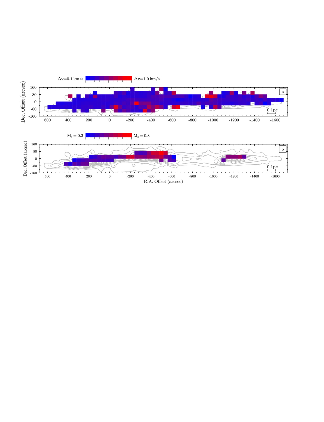
Figure 10: (a) Linewidths, $\Delta v$, of the ammonia (1,1) lines (FWHP) measured toward the core L1251A. (b) Mach numbers, $M_{s}$, of non-thermal motions at the 54 positions where $T_{\rm kin}$ was measured directly from the relative population of the (1,1) and (2,2) energy levels of NH₃. The contours are as in Fig. 3. The (0,0) map position is as in Fig. 1.

The coherence also leads to the nearly thermal NH₃ linewidths, which do not vary much in the interior of ammonia maps (and which are usually narrower than the linewidths of the surrounding C¹⁸O and ¹³CO gas), and transonic to subsonic velocity dispersions (e.g., Smith et al. 2009). We explore these issues in Fig. 10. Panel (a) shows a dominant linewidth $\Delta v\sim 0.2$ km s^-1, which is very close to the thermal broadening of NH₃ at a kinetic temperature $T_{\rm kin}$ = 10 K: $\Delta v_{\rm th}\approx 0.16$ km s^-1 (Eq. (A.6) in L13). The hyperfine structure fit to the NH₃(1,1) multiplet yields a maximum optical depth of $\sim 1$ for the isolated hfs component $F^{\prime}_{1}\to F^{\prime},F^{\prime}\to F=0\to 1,1/2\to 3/2$ at the offset (120″,$-40$″), suggesting negligible ($<20$%) optical depth broadening. Thus, the non-thermal motions do not dominate the thermal motions along the main axis E$\to$W of the filament.

However, approximately five times larger linewidths $\Delta v\sim 1$ km s^-1 were detected at a few points spread over the northern and southern ridges of the filament and in the vicinity of the outlier at the offset ($-200\arcsec,-40\arcsec$) with a maximum $\Delta v=1.0(1)$ km s^-1 at $(\Delta\alpha,\Delta\delta)=(-240\arcsec,-40\arcsec)$. The increasing contribution of the non-thermal motions to the NH₃ linewidths at the filament bounds correlates with the dynamics of the surrounding C¹⁸O and ¹³CO gas, showing $\Delta v({\scriptscriptstyle{\rm C}^{18}{\rm O}})=1.3$ km s^-1 and $\Delta v({{}^{13}{\rm CO}})=1.9$ km s^-1 at a mean excitation temperature of 10 K (S94). At this temperature, the thermal width of the carbon monoxide molecules is $\Delta v_{\rm th}\sim 0.12$ km s^-1, i.e., non-thermal motions such as infall, outflow, or turbulence dominate over the thermal motions in the outskirts of the filament. Therefore, the internal (C¹⁸O) and external (¹³CO) gas envelopes have a dynamical behavior that differs from that of the central ammonia string.

We also note that there are no visible correlations between the distribution of the NH₃ linewidths on the ammonia map in Fig. 10a and the directions of the jet and bipolar nebula outflows that are shown in Fig. 5. This can be understood if the axes of both jet and bipolar nebula were almost orthogonal to the line of sight.

Another way of looking at velocity coherence is to consider distributions of the Mach number defined locally as

$$M_{s}=\sigma_{\rm turb}/c_{s}\ ,$$ (5)

where $\sigma_{\rm turb}$ is the non-thermal velocity dispersion derived from the apparent line width (Eq. (A.7) in L13), and $c_{s}$ is the thermal sound speed

$$c_{s}=0.06\sqrt{T_{\rm kin}}\ ({\rm km}\leavevmode\nobreak\ {\rm s}^{-1})\$$ (6)

for an isothermal gas (Eq. (A.8) in L13).

Figure 10b shows the distribution of the calculated Mach numbers at the 54 positions where $T_{\rm kin}$ was measured directly from the relative population of the NH₃(1,1) and (2,2) energy levels. Panel (10b) demonstrates that the ratio of the non-thermal velocity dispersion to the sound speed along the main axis E$\to$W lies in the interval $0.3\;\raise 1.29167pt\hbox{$<$\kern-7.5pt\raise-4.73611pt\hbox{$\sim$}}\;M_{s}\;\raise 1.29167pt\hbox{$<$\kern-7.5pt\raise-4.73611pt\hbox{$\sim$}}\;0.8$; i.e., the filament has subsonic internal velocity dispersion in the coherent velocity region embedded in a generally supersonic turbulent envelope characterized by $M_{s}({\scriptscriptstyle{\rm C}^{18}{\rm O}})\sim 3$ and $M_{s}({{}^{13}{\rm C}{\rm O}})\sim 4$.

Finally, we conclude that the filament consists of at least three kinematically distinguished fragments with respect to their motion around the horizontal E$\to$W axis ($\alpha\beta$, bar, and $\gamma$ fragments), while all of them are involved in a common rotation around the vertical axis S$\to$N. The $\alpha\beta$ and $\gamma$ fragments spin around the E$\to$W axis in opposite directions that can be ascribed to dextral and sinistral chiralities. The bar shows no revolution, whereas the motion of the whole ammonia filament around the S$\to$N axis resembles a simple solid-body rotation. All these properties imply that the filament is kinematically detached from the outer layer traced by ¹³CO emission. The revealed coherence in the spatial and velocity distributions may, as usually supposed, be the manifestation of the intermittency of turbulent dissipation in molecular clouds connected with processes of star formation (e.g., Hennebelle & Falgarone 2012). The opposite chirality of the substructures in L1251A puts it in a list of fascinating objects that show a filamentary structure of a complex helix-like geometry (Carlqvist 2005).

3.3 Mass of the filament

The mass of NH₃ gas can be estimated from the dynamical characteristics and linear scale of the filament. If the cloud rotates as a solid body, the total mass of the ammonia filament stems from equilibrium of the centrifugal and gravitational forces:

$${\cal M}_{\rm tot}=(\Omega^{\scriptscriptstyle\rm SN}_{\rm tot})^{2}R^{3}/G\ ,$$ (7)

where $G$ is the gravitational constant, and $R$ is the radius along the major axis at which the linear velocity $V=\Omega R$ is measured. For $\Omega^{\scriptscriptstyle\rm SN}_{\rm tot}=7\times 10^{-15}$ rad s^-1 and $R\approx 1.65$ pc, one finds ${\cal M}_{\rm tot}\approx 45{\cal M}_{\odot}$. A two times higher mass was derived from the C¹⁸O data in S94 for cores A and B: ${\cal M}_{\scriptscriptstyle\rm A}\approx 56{\cal M}_{\odot}$, and ${\cal M}_{\scriptscriptstyle\rm B}\approx 38{\cal M}_{\odot}$.

If the considered object is an ellipsoid of revolution with axes $\ell_{1},\ell_{2},\ell_{3}$, then its volume is ${\cal V}=\frac{\pi}{6}\ell_{1}\ell_{2}\ell_{3}$, and for a uniform medium of mean density $\langle\rho\rangle$, its mass is ${\cal M}={\cal V}{\langle\rho\rangle}$. Substituting numerical values for $\ell_{1},\ell_{2},\ell_{3}$ and for ${\cal M}={\cal M}_{\rm tot}$, and using a mean molecular weight $\mu=2.33$, we find the mean gas number density ${\langle n\rangle}_{\scriptscriptstyle\rm H}={\langle\rho\rangle}/\mu m_{\scriptscriptstyle\rm H}=5.5\times 10^{3}$ cm^-3, where $m_{\scriptscriptstyle\rm H}$ is the mass of the hydrogen atom. A similar estimate, ${\langle n\rangle}=6.0\times 10^{3}$ cm^-3, is obtained if we adopt the rod-like geometry introduced in Sect. 3.1.

These gas densities are almost an order of magnitude lower than the ${\langle n\rangle}_{\scriptscriptstyle\rm H_{2}}\sim 4\times 10^{4}$ cm^-3 derived from ammonia emission along the major axis — a fact suggesting that there should be a gas number density gradient along the minor axes. Usually, the shape of a filament radial profile is described by a Plummer-like function of the form:

$$\rho(r)={\rho_{c}}/{\left[1+(r/r_{0})^{2}\right]^{\kappa/2}}\ ,$$ (8)

where $\rho_{c}$ is the central density of the filament, and $r_{0}$ is the radius in the plane orthogonal to the major axis (André et al. 2014).

For an isothermal gas cylinder in hydrostatic equilibrium, the power-law exponent of the density profile is $\kappa=4$ and $n(r)\propto r^{-4}$ (Ostriker 1964). However, observed filaments often show $n(r)\propto r^{-2}$, i.e., $\kappa\approx 2$ (e.g., Lada et al. 1999), suggesting that dense filaments may not be strictly isothermal but better described by a polytropic equation of state, $P(r)\propto\rho(r)^{\gamma}$ or $T(r)\propto\rho(r)^{\gamma-1}$ with $\gamma\;\raise 1.29167pt\hbox{$<$\kern-7.5pt\raise-4.73611pt\hbox{$\sim$}}\;1$ (Palmeirim et al. 2013).

It is easy to show that our case also requires $\kappa\approx 2$ to match the aforementioned estimates of the gas number densities $\langle n\rangle_{\scriptscriptstyle\rm H}$ and ${\langle n\rangle}_{\scriptscriptstyle\rm H_{2}}$. Thus, the filament L1251A is centrally condensed along its major axis, the NH₃ substructure is the densest part of it, its density profile is close to the Plummer model with $\kappa\approx 2$, and the total mass of the ammonia substructure is about $45{\cal M}_{\odot}$.

3.4 Gravitational equilibrium

The bound prestellar filaments are usually gravitationally unstable and prone to forming fragments (e.g., André et al. 2014). A self-gravitating cylinder will be in hydrostatic equilibrium only when its mass per unit length,

$${\cal M}_{\ell}=\int^{r_{0}}_{0}2\pi r\rho(r)dr\ ,$$ (9)

has the special critical value (Ostriker 1964):

$${\cal M}_{\ell,c}=\frac{2c^{2}_{s}}{G}=\frac{2kT}{G\mu m_{\scriptscriptstyle{\rm H}}}\approx 16.5T_{10}{\cal M}_{\odot}{\rm pc}^{-1}\ ,$$ (10)

where $c_{s}$ is the isothermal sound speed, and $T_{10}$ the gas temperature in units of 10 K. Since the mean molecular weight $\mu=2.33$ is expected to be almost constant in the interstellar molecular clouds, the critical line mass ${\cal M}_{\ell,c}$ is independent of the gas density and determined only by the kinetic temperature $T_{\rm kin}$.

If the mass per unit length ${\cal M}_{\ell}$ is equal to ${\cal M}_{\ell,c}$, then the self-gravitational force per unit mass and the pressure gradient force per unit mass are equal. If ${\cal M}_{\ell}<{\cal M}_{\ell,c}$, then a filament expands until it is supported by external pressure. Otherwise, when ${\cal M}_{\ell}>{\cal M}_{\ell,c}$, the filamentary structure is gravitationally unstable, and self-gravity dominates the pressure force. In this case, if ${\cal M}_{\ell}\gg{\cal M}_{\ell,c}$, perturbations do not grow much and the filament collapses toward the major axis without fragmentation (Inutsuka & Miyama 1992; Inutsuka & Miyama 1997).

Adopting ${\langle T\rangle}_{\rm kin}\approx 10$ K (Sect. 3.1), one finds a critical mass per unit length for the ammonia filament of ${\cal M}_{\ell,c}\approx 17{\cal M}_{\odot}{\rm pc}^{-1}$. Taking into account that the volumes of condensations ${\cal V}_{\alpha\beta}\approx{\cal V}_{\gamma}$, their mean gas densities ${\langle n\rangle}_{\alpha\beta}\approx 2{\langle n\rangle}_{\gamma}$, and the projected lengths $\ell_{\alpha\beta}\approx 2.2$ pc, $\ell_{\gamma}\approx 1.1$ pc (Sect. 3.1), the masses of the $\alpha\beta$ and $\gamma$ condensations are equal to ${\cal M}_{\alpha\beta}\sim 30M_{\odot}$ and ${\cal M}_{\gamma}\sim 15M_{\odot}$. This gives the line masses of ${\cal M}_{\ell,\alpha\beta}={\cal M}_{\ell,\gamma}\sim 14{\cal M}_{\odot}{\rm pc}^{-1}$. Thus, the masses per unit length are less than or comparable to ${\cal M}_{\ell,c}$ which is expected for gas in hydrostatic equilibrium.

4 Discussion

From the analysis of the dynamical stability of dark cloud L1251, Sato et al. (1994) concluded that all five C¹⁸O cores embedded in molecular gas (see Fig. 1) are gravitationally stable. The present observations in NH₃ inversion lines revealed that two of them, the cores A and B, have an elongated filament-like morphology and a complex velocity field. The filament exists for about $10^{7}$ yr and exhibits two types of global motions: ($i$) it rotates as a whole around the minor S–N axis, and ($ii$) its eastern and western fragments revolve around the major E–W axis in opposite directions of dextral and sinistral chirality. By analogy with the $\alpha$-$\omega$ geodynamo mechanism with broken symmetry (see, e.g., Fig. 2 in Love 1999), we suggest that these kinds of motions in L1251A may be maintained by helical magnetic fields threaded through the cloud.

Dynamo is a mechanism that converts kinetic energy into electromagnetic energy. The motion of an electrical conductor through a magnetic field induces electrical currents that can generate secondary induced magnetic fields that are sustained as long as energy is supplied. A self-exciting dynamo requires no external fields or currents to sustain the dynamo, aside from a weak seed magnetic field to get started. The $\omega$-effect is a conversion of poloidal field to toroidal that is caused by differential rotation (shear) of toroidal flows on the cloud surface. The $\alpha$-effect is a regeneration of the poloidal field from toroidal field due to upwelling poloidal flows possessing vorticity.

In this picture, the central region of L1251A (the bar between the eastern and western fragments), which shows no revolution, is the place where the helical magnetic field wrapped around the filament changes polarity from negative and positive. As a result we observe the eastern and western fragments revolving in opposite directions.

The physical parameters measured in L1251A allow us to evaluate the efficiency of the $\alpha$-$\omega$ dynamo mechanism. The importance of magnetic induction relative to magnetic diffusion is characterized by the magnetic Reynolds number (e.g., Brandenburg & Subramanian 2005):

$$R_{\rm m}=\sigma_{\rm rms}/({\tilde{\eta}}{\tilde{k}})\ ,$$ (11)

where $\sigma_{\rm rms}$ is the typical rms velocity, ${\tilde{\eta}}$ the resistivity (cm² s^-1 in cgs units), and ${\tilde{k}}=2\pi/{\ell}$ is the wavenumber. If, for numerical estimate, we take for ${\tilde{k}}$ a lower limit on the size of eddies close to the molecular mean free path in a dense core, $\ell=(\sqrt{2}n\sigma)^{-1}\sim 6\times 10^{-9}$ pc (the effective cross section $\sigma\sim 10^{-15}$ cm², the gas density $n\sim 4\times 10^{4}$ cm^-3), then ${\tilde{k}}\sim 4\times 10^{-10}$ cm^-1.

In dark clouds the gas is mostly neutral with low kinetic temperatures. In this case, the resistivity is given by (e.g., Balbus & Terquem 2001):

$${\tilde{\eta}}=234x^{-1}_{\rm e}T^{1/2}\ ,$$ (12)

where $x_{\rm e}=n_{\rm e}/n$ is the ionization fraction, and $n$ the number density of neutral particles.

If gas is shielded well from the external incident radiation, the gas temperature mainly comes from the heating by cosmic rays. Then the value of temperature is determined by the balance between heating and cooling. If the only source of heating are the cosmic rays and the cooling comes from the line radiation, then a lower bound on the kinetic temperature is about 8 K (Goldsmith & Langer 1978).

The ionization fraction $x_{\rm e}$ at the ionization-recombination equilibrium is approximately given by (e.g., Draine et al. 1983):

$$x_{\rm e}=(\zeta_{\scriptscriptstyle\rm CR}/{\tilde{\beta}}n)^{1/2}\ ,$$ (13)

where $\zeta_{\scriptscriptstyle\rm CR}$ is the ionization rate by cosmic rays, and ${\tilde{\beta}}=3\times 10^{-6}T^{-1/2}$ cm³ s^-1 is the dissociative recombination rate. Adopting the midplane value of $\zeta_{\scriptscriptstyle\rm CR}\approx 10^{-17}$ s^-1 (e.g., Sano & Stone 2002) and the measured mean temperature $T_{\rm kin}$$\approx 10$ K for the ionization rate due to cosmic rays, we find $x_{\rm e}\sim 2\times 10^{-8}$, so that ${\tilde{\eta}}\sim 4\times 10^{10}$ cm² s^-1. Then for $\sigma_{\rm rms}\sim 0.1$ km s^-1, we estimate the magnetic Reynolds number $R_{\rm m}\;\raise 1.29167pt\hbox{$>$\kern-7.5pt\raise-4.73611pt\hbox{$\sim$}}\;600$.

To control bulk motions, magnetic and non-thermal energy densities should be comparable,

$$B^{2}/8\pi\sim\rho\sigma^{2}_{\rm rms}/2\ ,$$ (14)

where $\rho$ is the gas density, and $\sigma_{\rm rms}$ the rms non-thermal (turbulent) velocity. With $\sigma_{\rm rms}\sim 0.1$ km s^-1 and $\rho=\mu m_{\scriptscriptstyle\rm H}n_{\scriptscriptstyle\rm H}\sim 3\times 10^{-19}$ g cm^-3, the mean equipartition strength of the magnetic field for the filament L1251A is expected to be $\langle B\rangle\sim 20$ $\mu$G, which is a typical value of $B$ measured in dark clouds (e.g., Crutcher 2012).

To amplify a dynamically significant magnetic field from a background initially weak seed field in a self-gravitating system, the gas must persist for a number of free-fall times, which is (e.g., McKee, & Ostriker 2007)

$$t_{ff}=\left(\frac{3\pi}{32G\langle\rho\rangle}\right)^{1/2}\sim 2\times 10^{5}\leavevmode\nobreak\ {\rm yr}\ ,$$ (15)

for L1251A. The value of $t_{ff}$, together with the estimated periods of the filament spinning ($t\sim 10^{7}$ yr) and the age of the supernova remnants ($t\sim 10^{6-7}$ yr), indicates that there has been plenty of time for the magnetic field to build up in the filament.

Theoretically, it has been suggested that a number of processes induce and maintain magnetic fields in dark clouds. Among them, mechanisms of a linear growth with time of the interstellar seed field from $B\sim 1$ $\mu$G to a typical $B\sim 20$ $\mu$G inside dark clouds are associated with a winding-up of frozen-in fields. Their efficiency is proportional to the number of rotations. Since the period for a complete rotation of the filament L1251A is comparable to its lifetime, which should be near the age of the supernova remnants, this type of mechanism can be excluded.

Other processes are based on an exponential growth that is realized in a dynamo amplification due to shear flows, turbulent, and Coriolis motions. The exponential growth can, in principle, strengthen the magnetic field on a timescale that resembles the filament rotation period. In case L1251A, different stages of the filament formation may be characterized by different types of magnetic field growth. In the first stages, when supernovae shock waves hit the cloud and caused strong turbulence, weak seed magnetic fields were exponentially amplified by the small-scale turbulent dynamo (e.g., Beresnyak & Lazarian 2015). At present, turbulent motions in the centrally condensed gas along the major axis are subsonic so that the turbulent dynamo is less effective. On the other hand, complex kinematics of L1251A and differential rotation may cause the Coriolis forces that tend to organize gas motions and electric currents into large scale Taylor columns (Taylor 1923) aligned with the rotation axis that, in turn, lead to induction of a magnetic field similar to the $\omega$-dynamo effect. The Taylor columns are formed when the Coriolis force is far more significant than the inertia force. The ratio between these two forces is characterized by the Rossby number, which is a dimensionless ratio of the inertia force over the Coriolis force:

$${\cal R}=v/L\Omega\ ,$$ (16)

where $v$ is the velocity of a parcel of fluid (a small amount of higher density fluid), $L$ is its scale (diameter), and $\Omega$ is the angular rotation. If the filament rotates more quickly than the parcel moves through it (i.e., ${\cal R}<1$), the gas flow is dragged across the filament at right angles to the spin axis and, thus, lifts and twists magnetic field lines, which is a similar process to the $\alpha$-dynamo effect. Both $\alpha$- and $\omega$-dynamo can maintain the strength of the magnetic field close to the equilibrium value given by Eq. (14).

5 Conclusions

Three hundred positions toward the C¹⁸O cores A and B within the dark cometary-shaped cloud L1251 were observed in the NH₃(1,1) and (2,2) inversion lines with the Effelsberg 100-m telescope at a spectral resolution of 0.045 km s^-1 and a spatial resolution of 40″. The main results are summarized as follows.

1. For the first time, we detect in L1251 a long and narrow structure covering a $38^{\prime}\times 3^{\prime}$ angular range ($\sim 3.3$ pc $\times$ 0.3 pc) in the E–W direction. The integrated ammonia intensity distribution is not homogeneous but concentrated in three condensations ($\alpha,\beta$, and $\gamma$) which form a rod-like filament. All of them are involved in a common rotation around the vertical S–N axis with angular velocity $\Omega^{\scriptscriptstyle\rm SN}_{\rm tot}\approx 7\times 10^{-15}$ rad s^-1.

2. The condensations exhibit a complex dynamical behavior: combined $\alpha$ and $\beta$ fragments are counter-rotating around the major E–W axis with respect to the ¹³CO envelope of the filament, whereas the $\gamma$ fragment co-rotates with this envelope. For both of them, the angular velocity is $|\Omega^{\scriptscriptstyle\rm EW}|\approx 2\times 10^{-14}$ rad s^-1. The central part of the filament between these two kinematically distinct regions does not show any rotation around the E–W axis.

3. The dextral and sinistral chirality of the $\alpha\beta$ and $\gamma$ condensations indicates the presence of magnetic field helicity of two types, negative and positive, supported by dynamo action.

4. An exclusive feature of the filament is extremely narrow ammonia lines observed at several “quiet zones” where the linewidths are $\Delta v\sim 0.1$ km s^-1, meaning that they reveal almost purely thermal broadening at kinetic temperatures as low as $\sim 8$ K.

5. Along the major E–W axis, we observed both the NH₃(1,1) and (2,2) transitions at 54 positions and found the mean ammonia column density ${\langle N\rangle}_{\scriptscriptstyle\rm NH_{3}}=(1.03\pm 0.05)\times 10^{15}$ cm^-2 and the gas number density ${\langle n\rangle}_{\scriptscriptstyle\rm H_{2}}=(3.9\pm 1.3)\times 10^{4}$ cm^-3 under the assumption that the beam filling factor $\eta=1$. The mean kinetic temperature is $\langle T_{\rm kin}\rangle=10.12\pm 0.08$ K.

6. The central part of the filament is organized into a coherent structure akin to those found in some other star-forming dense cores.

7. The Mach numbers calculated at the 54 positions within the coherent velocity region range between 0.3 and 0.8, which means that the filament shows subsonic internal velocity dispersion. The coherent velocity region is embedded in a generally supersonic turbulent envelope with Mach numbers $\sim 3-4$ as derived from observations of ${\rm C}^{18}{\rm O}$ and ${}^{13}{\rm C}{\rm O}$ lines.

8. The filament L1251A is centrally condensed along the E–W axis, the NH₃ substructure is the densest part of it, the density profile is close to the Plummer model with the power-law exponent $\kappa\approx 2$, and the total mass of the ammonia substructure is ${\cal M}\sim 45{\cal M}_{\odot}$.

9. The line masses ${\cal M}_{\ell}$ of the $\alpha\beta$ and $\gamma$ condensations ${\cal M}_{\ell,\alpha\beta}={\cal M}_{\ell,\gamma}\sim 14{\cal M}_{\odot}{\rm pc}^{-1}$ are less than or comparable to the critical value of ${\cal M}_{\ell,c}\sim 17{\cal M}_{\odot}{\rm pc}^{-1}$ which is expected for gas in hydrostatic equilibrium.

Helical magnetic fields aligned with the spin E–W axis play an important role in the evolution of the filament. The magnetic Reynolds number $R_{\rm m}\;\raise 1.29167pt\hbox{$>$\kern-7.5pt\raise-4.73611pt\hbox{$\sim$}}\;600$ means that magnetic induction dominates magnetic diffusion, a condition required for $\omega$-dynamos. The Rossby number ${\cal R}<1$ indicates that the Taylor columns are dragged across the filament leading to the $\alpha$-dynamo effect. The joint action of both the $\omega$- and $\alpha$-dynamo mechanisms can provide a large scale magnetic field of positive and negative helicity that, in turn, results in the observed gas motions of opposite chirality.

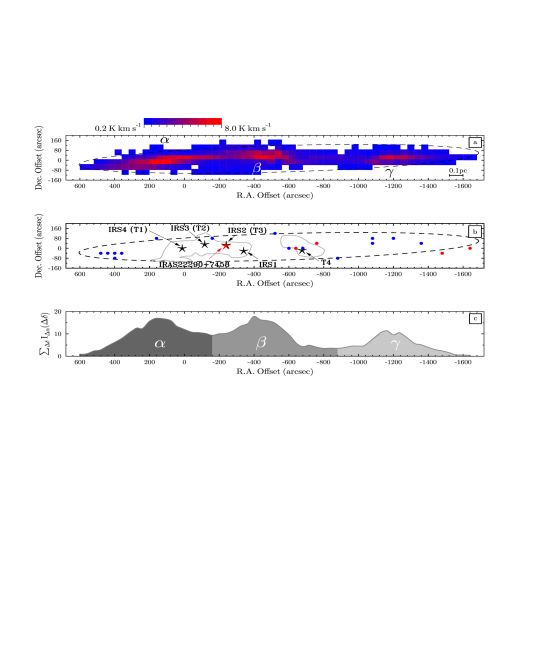
Figure 2: (a) NH₃(1,1) integrated intensity map ($\int$$T_{\scriptscriptstyle\rm MB}$$dv$ in units of K km s^-1) of the molecular core L1251A. Each color box has a size of $40^{\prime\prime}\times 40^{\prime\prime}$, and its bottom left corner corresponds to the telescope pointing. The parameters of the NH₃ peaks $\alpha,\beta$, and $\gamma$ are given in Table 1. The core exhibits a filamentary structure that can be enveloped by an ellipse (dashed line) with principal axes of 1140″ and 89″. (b) Schematic configuration of the filament and peak positions of the ammonia cores T1–T4. The gray contours restrict ammonia emission to the lowest level of the integrated NH₃(1,1) emission as in Fig. 3 in Tóth & Walmsley (1996). The location of the IRS sources are from Lee et al. (2010). The red star is the IR source detected by IRAS. The filled blue and red circles outline areas of the narrowest ammonia lines with FWHP line widths of, respectively, $\Delta v\sim 0.2$ km s^-1, and $\sim 0.1$ km s^-1; their offsets are listed in Table 1. (c) The sum over the integrated intensities for a given R.A., $\sum_{\Delta\delta}I_{\Delta\alpha}(\Delta\delta)$. The (0,0) map position and the distance to the source are as in Fig. 1.

Table 1: Peak intensities of NH₃(1,1) line emission and positions of the narrowest lines toward L1251 A and B.

Peak	Offsetb		$T_{\scriptscriptstyle\rm MB}$c	$V_{\scriptscriptstyle\rm LSR}$		$\Delta v$
IDa	$\Delta\alpha$,	$\Delta\delta$	(K)	(km s-1)		(km s-1)
	(″),	(″)				(FWHP)
$\alpha$	$160$,	$-40$	4.5(5)	$-4$.	212(3)	0.	260(8)
$\beta$	$-400$,	$0$	3.7(4)	$-3$.	922(4)	0.	34(1)
$\gamma$	$-1160$,	$0$	3.3(3)	$-3$.	819(4)	0.	30(1)
	$-720$,	$0$	2.2(2)	$-3$.	984(6)	0.	24(1)
	$-1640$,	$0$	0.8(1)	$-3$.	69(2)	0.	14(3)
	$-1480$,	$-40$	0.9(1)	$-3$.	67(1)	0.	10(2)
	$-1360$,	$40$	0.7(1)	$-3$.	82(1)	0.	21(3)
	$-1200$,	$80$	0.7(1)	$-4$.	12(3)	0.	20(4)
	$-1080$,	$80$	0.4(1)	$-4$.	20(2)	0.	18(5)
	$-1080$,	$40$	0.8(1)	$-4$.	11(2)	0.	20(3)
	$-880$,	$-80$	0.4(1)	$-3$.	77(3)	0.	18(4)
	$-760$,	$40$	0.7(1)	$-4$.	03(1)	0.	12(2)
	$-680$,	$0$	1.4(1)	$-3$.	999(5)	0.	20(2)
	$-640$,	$0$	1.3(1)	$-3$.	999(3)	0.	13(2)
	$-600$,	$0$	2.3(2)	$-4$.	002(5)	0.	21(1)
	$-520$,	$120$	0.5(1)	$-4$.	19(3)	0.	16(5)
	$-160$,	$80$	0.5(1)	$-4$.	26(2)	0.	19(3)
	$160$,	$80$	0.5(1)	$-4$.	18(3)	0.	17(4)
	$360$,	$-40$	2.8(3)	$-4$.	303(4)	0.	21(1)
	$400$,	$-40$	2.0(2)	$-4$.	318(6)	0.	21(1)
	$400$,	$-80$	2.8(3)	$-4$.	334(4)	0.	22(1)
	$440$,	$-40$	1.9(2)	$-4$.	298(7)	0.	21(2)
	$480$,	$-40$	1.1(1)	$-4$.	31(1)	0.	19(2)
Notes. aGreek letters label the peaks of ammonia
emission indicated in Fig. 2. bThe zero offset (0,0) is
R.A. = 22:31:02.3, Dec = 75:13:39 (J2000).
cThe numbers in parentheses correspond to a $1\sigma$
statistical error on the last digit.