Complete cosmic scenario in the Randall-Sundrum braneworld from the dynamical systems perspective

Abstract

The paper deals with dynamical system analysis of a coupled scalar field in the Randall-Sundrum(RS)2 brane world. The late time attractor describes the final state of the cosmic evolution. In RS2 based phantom model there is no late-time attractor and consequently there is uncertainty in cosmic evolution. In this paper, we have shown that it is possible to get late-time attractor when gravity is coupled to scalar field. Finally, in order to predict the final evolution of the universe, we have also studied classical stability of the model. It is found that there are late time attractors which are both locally as well as classically stable and so our model can realise the late time cosmic acceleration.

Keywords : RS braneworld; phantom scalar field ; dynamical system; attractor; phase space.

I Introduction

The modified theories of gravity which can explain the present observed accelerated expansion of the universe sp ; sp03 ; ag without any need of dark energy(DE) ejc ; kbamba have received lot of success in recent years. Brane gravity(BG)/Braneworld scenario inspired by advances of String/M-Theory is a prominent theory of modified gravity. In this scenario our observable universe is assumed to be a sub-manifold embedded in compactified higher dimensional space time known as bulk. Here except gravity, all the standard model particles are confined to sub- manifold called brane. Braneworld models provides a novel way to correct General Relativity(GR) and gives answer to several unsolved problems of cosmology rm .

Among different braneworld models, the Randall-Sundrum type II model(RS2) is very popular among cosmologists due to its rich conceptual base rs2 . RS2 model gave a framework often referred as braneworlds with wrapped extra-dimension in contrast to Kaluza-Klein mechanism of compactification where extra-dimension is very small rs1 . In this set up big-rip singularity of phantom model can be avoided and acceleration is transient in nature sksjd . In contrast to GR based models here inflation is possible for a large class of potentials due to modified Friedmann equationrmhawkins .

Another braneworld model that received considerable attention is the Dvali-Gabadadze-Porrati(DGP) braneworld model dgp1 ; dgp2 ; dgp3 . This model can explain the present acceleration without using mysterious DE. Usually RS2 model modifies GR at small cosmological scales and DGP model modifies GR at large cosmological distance. Consequently RS2 models have more impact on cosmology of early universe. The interesting and recent feature is that RS2 model can also modify late time cosmic expansion if the energy density of the matter content increases at late time e.g., phantom scalar field sksjd ; GarciaSalcedo:2010wa . Thus for scalar fields like phantom, RS2 models can have impact on late universe and it can give a complete cosmic scenario.

Dynamical systems tools have a central role for qualitative analysis of homogeneous cosmological models whose evolution is governed by finite dimensional autonomous system of ordinary differential equations (ASODE) dsincosmology ; Coley:2003mj . The goal of the dynamical systems approach is to correlate asymptotic cosmological solutions with important concepts like past and future attractors along with saddle points. In the phase space of models, if a critical point can be associated with a solution, it means that in the neighbourhood of this solution the universe dynamics will evolve for a sufficiently long time irrespective of initial data. To describe a complete cosmological scenario, a cosmological model described by an autonomous system must have a past time attractor (to represent inflationary epoch), one or two saddle points (to represent radiation and matter dominated universe) and an late time attractor (to represent accelerated expansion universe) Boehmer:2014vea .

In cosmology scalar fields play an active role to model DE, inflation and other cosmological features ar ; jm . The dynamical study of a scalar field coupled with perfect fluid has found many applications in GR context. For a nice introduction Boehmer:2014vea ; ir1 and application of this technique in GR based cosmology one can see recent papers nroy1 ; nroy ; nrn1 . In RS2 model, using dynamical system approach Rudra $et$ $al$ investigated role of modified Chaplyging gas in explaining accelerated expansion of the universe prudra . They showed that around fixed points universe expands with a power-law. A dynamical study of Dirac Born Infield (DBI) trapped in the braneworld is explored in arx and it is found that in ultra relativistic regime scalar field dominated and matter scaling solutions exist. In braneworld context dynamics of self-interacting scalar field trapped in a RS2 model for a wide variety of potentials have been studied in Gonzalez:2008wa ; Leyva:2009zz ; de . Escobar $et$ $al$ did a refined study of a scalar field trapped in RS2 model using Centre Manifold Theory with an arbitrary potential. They proved that there are no late time attractors with 5D modifications de . Furthermore, in a recent paper Biswas $et$ $al$ studied interacting dark energy in RS2 braneworld using dynamical systems tools Biswas:2015zka . All the above studies were done for a quintessence scalar field. It is found that only early times cosmology is modified with respect to GR based models. On the contrary for usual phantom scalar field, the higher dimensional Brane effects of RS2 usual phantom scalar field model modifies past and future asymptotic properties so that we get past time attractor and saddle point only GarciaSalcedo:2010wa . In GR based phantom scalar field model we get saddle point and late time attractor but it does not admit past time attractor GarciaSalcedo:2010wa ; BG .

In this paper we shall show that in RS2 model when gravity is coupled to scalar field with scalar coupling function and a potential, the late universe is also modified and we get a complete cosmic scenario. The coupling function additionally helps to control the behaviour of scalar field and have been used extensively in unifying phantom inflation with late time acceleration kbamba ; sn ; sc ; as . Recently Mahata $et$ $al$ Mahata:2013oza studied the dynamics of phantom cosmological model where gravity is coupled to scalar field having scalar coupling function in GR context using dynamical system tools. The aim of this paper is to study the dynamics of coupled scalar field on RS2 braneworld by using dynamical system tools. Furthermore, we have also examined the classical stability of the model in addition to calculating various observable quantities in the asymptotic solutions. In contrast to Ref Mahata:2013oza , we shall show that coupled scalar field give rich dynamics and late time acceleration solutions are also classically stable.

The paper is organised as follows: The basic and the evolution equations of the autonomous system are presented in section (II). Sections (III) and (IV) deals with the analysis of the critical points of the system in 4D and 3D respectively. The classical stability of the model has been studied in section (V). Final section is devoted to discussion and conclusion.

II Basic equations

The total action of the field equations in RS2 model is written as

$$S=S_{RS}+S_{\phi}+S_{m}$$ (1)

where

$$S_{RS}=\int d^{5}x~{}\sqrt{-g^{(5)}}~{}(2R^{(5)}+\Lambda_{5})+\int d^{4}x~{}\sqrt{-g}~{}\lambda$$ (2)

is the action of RS2 model,  $g^{(5)}_{\mu\nu}$ and $g_{\mu\nu}$ are the bulk metric and the brane metric respectively, $R^{(5)}$ is the Ricci scalar in the bulk and $\Lambda_{5}$ is the bulk cosmological constant, $S_{\phi}$ is the action of the scalar field coupled to gravity given by

$$S_{\phi}=\int d^{4}x\sqrt{-g}~{}\Big{[}~{}-\frac{1}{2}\mu(\phi)g^{\mu\nu}(\nabla_{\mu}\phi)(\nabla_{\nu}\phi)-V(\phi)~{}\Big{]}$$ (3)

$\mu(\phi)$ is the coupling parameter, $V(\phi)$ is the potential of the scalar field and $S_{m}=\int d^{4}x~{}\sqrt{-g}~{}L_{m}$ is the action of the matter field which is chosen as the cold dark matter (CDM).

Observations support homogeneous and isotropic model of the late universe, given by the line-element ad

$$ds^{2}=dt^{2}-a^{2}(t)[dx^{2}+dy^{2}+dz^{2}]$$ (4)

where $a(t)$ is the scale factor. In this space-time, from action (1) we get the following RS2 model based modified Friedmann field equations rm

$$3H^{2}=\rho_{T}\Big{(}1+\frac{\rho_{T}}{2\lambda}\Big{)}$$ (5)

Here $\lambda$ is the brane tension and $\rho_{T}=\rho_{\phi}+\rho_{m}$ , $\rho_{\phi}$ and $\rho_{m}$ are being the energy density of CDM and the scalar field respectively. It should be noted that we have neglected the cosmological constant in the $4$D brane by choosing RS fine tuning condition and for simplicity of calculation we have chosen AdS bulk where dark radiation term vanishes.

When gravity is coupled to the scalar field with scalar coupling function, the energy density and thermodynamic pressure are given by

$$\rho_{\phi}=\frac{1}{2}\mu(\phi)\dot{\phi}^{2}+V(\phi)\hskip 42.67912pt\textrm{and}\hskip 42.67912ptp_{\phi}=\frac{1}{2}\mu(\phi)\dot{\phi}^{2}-V(\phi)$$ (6)

where $\mu(\phi)$ is the coupling parameter chosen for arbitrary function of $\phi$ and $V(\phi)$ is the potential of the scalar field.

Here we assume that the scalar field does not interact with CDM and the energy conservation relations takes the form.

$$\dot{\rho_{\phi}}+3H(\rho_{\phi}+p_{\phi})=0$$ (7)

$$\dot{\rho_{m}}+3H\rho_{m}=0$$ (8)

Using Eqs.(5) , (6) , (7) and (8), we get

$$2\dot{H}=-\Big{(}1+\frac{\rho_{T}}{\lambda}\Big{)}(\mu(\phi)\dot{\phi}^{2}+\rho_{m})$$ (9)

This implies

$$\mu(\phi)\dot{\phi}^{2}=-\Big{(}\frac{2\dot{H}}{1+\frac{\rho_{T}}{\lambda}}+\rho_{m}\Big{)}$$ (10)

As clear from Eq.(10), when $\dot{H}$ is positive, we have phantom phase where $\mu(\phi)$ is negative and using conservation Eqs.(7) and (8), evolution equation of the scalar field is given by

$$\mu(\phi){\ddot{\phi}}+\frac{1}{2}\frac{d\mu(\phi)}{d\phi}\dot{\phi^{2}}+3H\mu(\phi)\dot{\phi}+\frac{dV}{d\phi}=0$$ (11)

Following Leyva:2009zz , we introduce the following dimensionless phase space variables in order to build ASODE of the above cosmological equation.

$$x\equiv\frac{\sqrt{\mu(\phi)}~{}\dot{\phi}}{\sqrt{6}~{}H},\hskip 5.69046pty\equiv\frac{\sqrt{V(\phi)}}{\sqrt{3}~{}H}\hskip 5.69046pt,\hskip 5.69046ptz\equiv\frac{\rho_{T}}{3H^{2}}\hskip 5.69046pt\textrm{and}\hskip 5.69046pts\equiv\frac{\sqrt{6}}{\phi}$$ (12)

After these choice of phase space variables, we can write following ASODE for above evolution equations

$$x^{\prime}=-3x-\beta_{1}(s)~{}y^{2}+\frac{3}{2}x\Big{(}\frac{2-z}{z}\Big{)}(z+x^{2}-y^{2})$$

$$y^{\prime}=\beta_{1}(s)~{}xy+\frac{3}{2}y\Big{(}\frac{2-z}{z}\Big{)}(z+x^{2}-y^{2})$$

$$z^{\prime}=3(1-z)+(z+x^{2}-y^{2})$$

$$s^{\prime}=-\frac{xs^{2}}{\sqrt{\mu_{1}(s)}}$$ (13)

where $\beta_{1}(s)=\beta(\phi)=\sqrt{\frac{3}{2\mu(\phi)}}~{}\frac{d\ln V}{d\phi}$ , $\mu_{1}(s)=\mu(\phi)$ and the primes denotes differentiation with respect to new time variable $U=\ln a$. After the above choice of variables one can realise that

$$\frac{\rho_{T}}{\lambda}=\frac{2(1-z)}{z},\;\Rightarrow\;0<z\leq 1$$ (14)

Eq.(14) tells us that at $z=1$, brane effects vanish and GR is recovered. It may be noted that at the point $z=0$ the ratio $\frac{\rho_{T}}{\lambda}$ is undefined but as we are interested in asymptotic behaviour, we can study the limiting case $z\rightarrow 0$ separately.

The effective equation of state for the scalar field (i.e. $p_{\phi}=(\nu_{\phi}-1)\rho_{\phi})$ is given by

$$\nu_{\phi}=\frac{2x^{2}}{x^{2}+y^{2}}$$ (15)

From the above dimensionless phase space variables the equation of state (EoS) parameter has the expression

$$\omega_{\phi}=\frac{p_{\phi}}{\rho_{\phi}}=\frac{x^{2}-y^{2}}{x^{2}+y^{2}}$$ (16)

The density parameter for the scalar field has the same expression as that of GR Mahata:2013oza

$$\Omega_{\phi}=x^{2}+y^{2}$$ (17)

Also we have

$$\Omega_{m}=z-x^{2}-y^{2}\hskip 34.14322pt\textrm{and}\hskip 34.14322ptq=-1-\frac{\dot{H}}{H^{2}}$$ (18)

where $\frac{\dot{H}}{H^{2}}=-\frac{3}{2}\Big{(}\frac{2-z}{z}\Big{)}(z+x^{2}-y^{2})$ so that the deceleration parameter $q$ has the expression

$$q=-1+\frac{3}{2}\Big{(}\frac{2-z}{z}\Big{)}(z+x^{2}-y^{2})$$ (19)

For numerical calculations we have estimated initial conditions in such a way that it is consistent with present observations ( $\Omega_{m}=0.27$ and the deceleration parameter $q=-0.53$ rg  ), so

$$\Omega_{\phi}=x^{2}_{0}+y^{2}_{0}=0.73$$ (20)

Using these values in the constraint Eq.(18), we get $z_{0}=1$, where $x_{0}$, $y_{0}$ and $z_{0}$ are the present values of $x$, $y$ and $z$ respectively. Eq.(19) and (20) yields a lower bound set of present work $x_{0}=0.489$ and $y_{0}=0.7$.

Here we see that the expressions of CDM energy density parameter and deceleration parameter involve brane effects and it differs from that of GR GarciaSalcedo:2010wa .

The phase space for the autonomous dynamical system driven by the evolution Eq.(13) can be defined as:

$$\Psi=\{(x,y,z):0\leq{x^{2}}+y^{2}\leq{z},-1\leq{x}\leq{1},0\leq{y},0<z\leq{1}\}\times\{s\in\mathbb{R}\}$$ (21)

III Critical points of 4D autonomous system

In this section we will analyse in detail the critical points of the autonomous system corresponding to RS2 model and their stability properties. Let $y^{\prime}=g(y)$ be a given non-linear autonomous system of differential equations with a critical point $y_{0}\in\mathbb{R}^{n}$, where $y^{\prime}=\frac{dy}{dt}$, $y\equiv(y_{1},y_{2},.......,y_{n})\in\mathbb{R}^{n}$ and $g:\mathbb{R}^{n}\rightarrow\mathbb{R}^{n}$. The system can be linearised around the critical point as $u^{\prime}=Au=Df(y_{0})u$, where $u=y-y_{0}$, $A=Df(y_{0})$ and $Df(y)=\frac{\partial g_{i}}{\partial y_{j}}$, $i,j=1,2,3,.......n$ and $A$ is the Jacobian matrix of the system. A critical point of the system is said to be hyperbolic if none of the eigenvalues of the Jacobian matrix $A$ have zero real part. If the Jacobian matrix have at least one zero eigenvalue, then the critical point is non-hyperbolic critical point. We summarise the stability criteria of the hyperbolic critical point which can be determined from the sign of eigenvalues of $A$ as follows:

• If all the eigenvalues have negative real part then the critical point is stable (i.e., late time attractor).

• If all the eigenvalues have positive real part then the critical point is unstable (i.e., past time attractor).

• If some eigenvalues of the Jacobian matrix have positive real part and other have negative real part then the critical point is saddle.

The above linear stability analysis cannot be used for non-hyperbolic points, so some other techniques such as Centre Manifold Theory, Lyapunov’s functions Boehmer:2014vea ; wigginsbook and numerically perturbation of solutions around critical points strogatz may be employed to study the stability of such points. The method of perturbations of solutions around critical points is quite standard and has been extensively used in recent cosmological studies nroy1 ; nroy ; nrn1 and so this technique will be used in our present work.

In order to solve the above ASODE (13) we need to consider specific potential $V(\phi)$ and coupling function $\mu(\phi)$. Regarding $V(\phi)$, the general popular choice in literature is to assume an exponential potential. This potential has the advantage that the phase space remains four dimensional and field equations can be studied easily qualitatively using dynamical systems tools. In order to consider $V(\phi)$ beyond the constant and exponential potential, one new variable $v\equiv\frac{1}{V}~{}\frac{dV}{d\phi}$ has to be introduced scc ; rj ; pj . Further, exponential potential in case of phantom field in standard cosmology admits late time attractor but in the RS2 model yields saddle point GarciaSalcedo:2010wa . In this paper we shall show that it is possible to get late time attractor under this potential in RS2 model when gravity is coupled to scalar field. As exponential potentials are known to be significant in dynamical investigations Copeland:1997 ; gleon ; hjj , we assume $V(\phi)=V_{0}e^{-\alpha\phi}$. Concerning coupling function $\mu(\phi)$, the popular choice in literature are exponential and power-law forms Mahata:2013oza ; gleonn . In what follows as in Mahata:2013oza , in order to remain general, we choose two coupling functions (exponential and power-law forms) corresponding to same the exponential potential and the corresponding analysis will be done separately in following two subsections.

III.1 Scenario 1 : Exponential potential and exponential coupling function

Here we choose

$$V(\phi)=V_{0}e^{-\alpha\phi}\hskip 34.14322pt\textrm{and}\hskip 34.14322pt\mu(\phi)=\mu_{0}e^{\nu\phi}$$ (22)

In this scenario, the autonomous system (13) simplifies to

$$x^{\prime}=-3x+\alpha_{0}~{}y^{2}\mathrm{e}^{-\frac{b}{s}}+\frac{3}{2}x\Big{(}\frac{2-z}{z}\Big{)}(z+x^{2}-y^{2})$$

$$y^{\prime}=-\alpha_{0}~{}xy\mathrm{e}^{-\frac{b}{s}}+\frac{3}{2}y\Big{(}\frac{2-z}{z}\Big{)}(z+x^{2}-y^{2})$$

$$z^{\prime}=3(1-z)(z+x^{2}-y^{2})$$

$$s^{\prime}=-\frac{xs^{2}~{}\mathrm{e}^{-\frac{b}{s}}}{\sqrt{\mu_{0}}}$$ (23)

where $\alpha_{0}=\alpha~{}\sqrt{\frac{3}{2\mu_{0}}}$ and $b=\sqrt{\frac{3}{2}}~{}\nu$
The critical points of the present autonomous system are:
$C_{1}(0,0,0,0)$ , $C_{2}(0,0,1,0)$ , $C_{3}^{\pm}(\pm 1,0,1,0)$ , $C_{4}(0,1,1,s)$ , $C_{5}(0,\sqrt{z},z,0)$ ,  $C_{6}(0,0,0,s)$ , $C_{7}(0,0,1,s)$

Table 1. Scenario $1$ : Exponential potential and exponential coupling function. The critical points for ASODE (23) and values of the relevant parameters

Critical point	x	y	z	s	Existence	${\Omega}_{\phi}~{}~{}~{}$	${\Omega}_{m}~{}~{}~{}$	${\omega}_{\phi}$
$C_{1}$	0	0	0	0	Always	0	0	Undefined
$C_{2}$	0	0	1	0	,,	0	1	Undefined
$C_{3}^{\pm}$	$\pm 1$	0	1	0	,,	1	0	1
$C_{4}$	0	1	1	0	,,	1	0	-1
$C_{5}$	0	$\sqrt{z}$	$z\in]0,1]$	0	,,	z	0	-1
$C_{6}$	0	0	0	s	,,	0	0	Undefined
$C_{7}$	0	0	1	s	,,	0	1	Undefined

Table 2. Scenario $1$ : Exponential potential and exponential coupling function. Eigenvalues of the linearised matrix for the critical points ASODE (23) and corresponding values of dimension of Stable manifold and deceleration parameters.

Critical point	$\lambda_{1}~{}~{}~{}$	$\lambda_{2}~{}~{}~{}$	$\lambda_{3}~{}~{}~{}$	$\lambda_{4}~{}~{}~{}~{}~{}$	Stable manifold	q
$C_{1}$	$0~{}~{}$	$3~{}~{}~{}$	$3~{}~{}~{}$	$0~{}~{}~{}~{}~{}$	No stable manifold	$2$
$C_{2}$	$-\frac{3}{2}~{}~{}~{}$	$\frac{3}{2}~{}~{}~{}$	$-3~{}~{}~{}$	$0~{}~{}~{}~{}~{}$	2D	$\frac{1}{2}$
$C_{3}^{\pm}$	$3~{}~{}$	$3~{}~{}~{}$	$-6~{}~{}~{}$	$0~{}~{}~{}~{}~{}$	1D	2
$C_{4}$	$-3~{}~{}$	$-3~{}~{}~{}$	$0~{}~{}~{}$	$0~{}~{}~{}~{}~{}$	2D	-1
$C_{5}$	$-3~{}~{}$	$-3~{}~{}~{}$	$0~{}~{}~{}$	$0~{}~{}~{}~{}~{}$	2D	-1
$C_{6}$	$0~{}$	$3~{}~{}~{}$	$3~{}~{}$	$0~{}~{}~{}~{}~{}$	No stable manifold	2
$C_{7}$	$-\frac{3}{2}~{}~{}~{}$	$\frac{3}{2}~{}~{}~{}$	$-3~{}~{}~{}$	$0~{}~{}~{}~{}~{}$	2D	$\frac{1}{2}$

III.1.1 Critical points and their properties for Scenario $1$:

The critical points of the above ASODE (23) and the eigenvalues of the corresponding Jacobian matrix are listed in Table $1$ and Table $2$ respectively. Here we see that all the critical points are non hyperbolic in nature. So linear stability theory cannot be used to study the stability of the system. But using centre manifold theorem we can find dimension of stable manifold in this case wigginsbook . It may be noted that the five dimensional effects are presented when $z\neq 1$ so $C_{1}$ , $C_{5}$ and $C_{6}$ only reflects the brane effects.

We note that the point $C_{1}=(0,0,0,0)$ is a critical point of the ASODE (23). But at this point the first two equations of ASODE (23) are undefined. To study the nature of the critical point $C_{1}$, we can apply a secure approach as reported in GarciaSalcedo:2010wa and expand ASODE (23) in the neighbourhood of $C_{1}=(0,0,0,0)$ by putting $x\rightarrow 0+\epsilon_{x}~{},~{}y\rightarrow 0+\epsilon_{y}~{},~{}z\rightarrow 0+\epsilon_{z}~{}$ and $~{}s\rightarrow 0+\epsilon_{s}$ in the above ASODE (23). If we neglect higher order terms, then the ASODE (23) reduces to following system $\epsilon^{\prime}_{x}=0~{},~{}\epsilon^{\prime}_{y}=3\epsilon_{y}~{},~{}\epsilon^{\prime}_{z}=3\epsilon_{z}$ and $\epsilon^{\prime}_{s}=0$. So, the point $C_{1}$ is non hyperbolic critical point. We can only say in this case is that the point $(0,0,0,0)$ is unstable as perturbations will grow exponentially. So this critical point will behave as past time attractor and is characterised by vanishing matter content and we have empty (Misner-RS) universe. In braneworld, existence of empty universe is a distinctive feature. Furthermore, we have a decelerating solution with $(q=2)$ (limiting case) at this point. The behaviour of $C_{6}$ is same as $C_{1}$ and $C_{3}$ is not interesting from physical point of view. In what follows we summarise the remaining critical points of scenario $1$ and their properties.

• As seen from Tables $1$ and $2$, the saddle critical points $C_{2}$ and $C_{7}$ indicate that universe is completely dominated by dark matter $(\Omega_{m}=1)$ and expansion of the universe around these points is decelerated $(q=\frac{1}{2})$ having 2D stable manifolds. These points are saddle in nature.

• At the critical point $C_{4}$, we see that the universe is completely dominated by the scalar field, at this point expansion of the universe is accelerated $(q=-1)$ having two negative eigenvalues and two zero eigenvalues. Since this point is non-hyperbolic, we numerically perturbed the solutions near this critical point and check the stability. To this end we plot the projections of perturbations on $x,y,z$ and $s$ axes separately in FIG.(1) to FIG.(4). From FIG.(1) and FIG.(4) we see that the projection of perturbations solutions asymptotically approach $x=0$ and $s=0$ respectively as $U$ approaches to infinity. Similarly, from FIG.(2) and FIG.(3), $y$ and $z$ approach to $1$ as $U$ approaches to infinity, so that the whole system asymptotically approach the critical point $C_{4}=(0,1,1,0)$ as $U$ approaches to infinity. From this perturbation plots we can conclude that the point $C_{4}=(0,1,1,0)$ is a stable critical point of the ASODE (23).

• For the critical point $C_{5}$, we have $(x,y,z,s)=(0,\sqrt{z},z,0)$. This implies $z=y^{2}~{}(x=0~{},~{}s=0)$, so that this point is a curves of critical points. If we compare $C_{4}$ and $C_{5}$, we see that $C_{4}$ is a particular case of $C_{5}$. At this point $\rho_{m}=0$ and $\rho_{T}=V$, so that the above Eq.(5) reduces to
  $3H^{2}=V~{}\Big{(}1+\frac{V}{2\lambda}\Big{)}$. It represents the slow-roll Friedmann equation where the Hubble parameter is related to the potential of the inflation field having 2D stable manifolds. When potential is much larger than the brane tension $V>>\lambda$ $\Rightarrow H_{RS}=\frac{V}{\sqrt{6\lambda}}$, so that at early time expansion rate $H_{RS}$ get enhanced with respect to the $H_{GR}$ ( GR rate of expansion) in the RS2 model and we have $\frac{H_{RS}}{H_{GR}}=\sqrt{\frac{V}{2\lambda}}$. Thus in this way brane effects fuel early inflation in RS2 model. FIG.(5) shows that the nature of curves of critical points of $C_{5}$

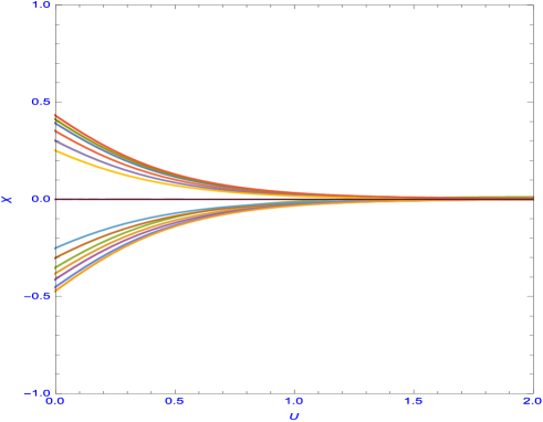
Figure 1: The plot of $X$ against $U$ for Scenario $1$ near the critical point $C_{4}$

.

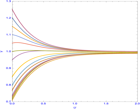
Figure 2: The plot of $Y$ against $U$ for Scenario $1$ near the critical point $C_{4}$

.

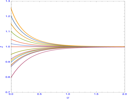
Figure 3: The plot of $Z$ against $U$ for Scenario $1$ near the critical point $C_{4}$

.

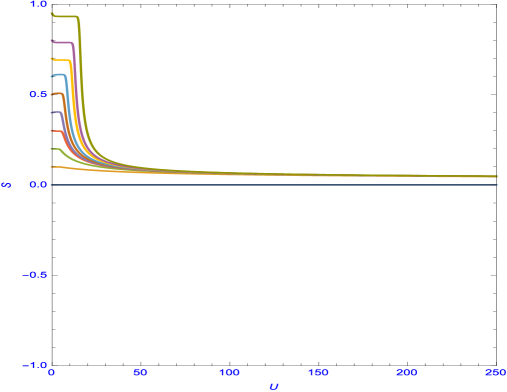
Figure 4: The plot of $S$ against $U$ for Scenario $1$ near the critical point $C_{4}$

.

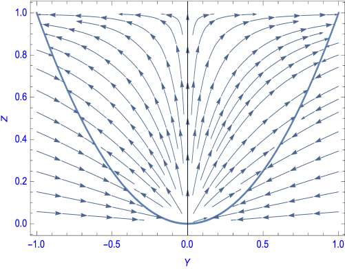
Figure 5: Phase portrait of Scenario $1$ near the critical point $C_{5}$

.

III.2 Scenario $2$ : Exponential potential and power law coupling parameter

Here we choose

$$V(\phi)=V_{0}e^{-\alpha\phi}\hskip 34.14322pt\textrm{and}\hskip 34.14322pt\mu(\phi)=\mu_{0}\phi^{n}$$ (24)

where $V_{0}$, $\mu_{0}$ and $n$ are constants.
Then the autonomous system (13) becomes

$$x^{\prime}=-3x+\beta_{2}~{}y^{2}s^{\frac{n}{2}}+\frac{3}{2}x\Big{(}\frac{2-z}{z}\Big{)}(z+x^{2}-y^{2})$$

$$y^{\prime}=-\beta_{2}~{}xys^{\frac{n}{2}}+\frac{3}{2}y\Big{(}\frac{2-z}{z}\Big{)}(z+x^{2}-y^{2})$$

$$z^{\prime}=3(1-z)(z+x^{2}-y^{2})$$

$$s^{\prime}=-\mu_{2}~{}xs^{2+\frac{n}{2}}$$ (25)

where $\beta_{2}=\alpha_{0}6^{-\frac{n}{4}}$ and $\mu_{2}=\frac{6^{-\frac{n}{4}}}{\sqrt{\mu_{0}}}$. The critical points of the present autonomous system are $D_{1}(0,0,0,0)$ , $D_{2}(0,0,1,0)$ ,  $D_{3}^{\pm}(\pm 1,0,1,0)$ , $D_{4}(0,1,1,s)$ , $D_{5}(0,\sqrt{z},z,0)$ , $D_{6}(0,0,0,s)$ , $D_{7}(0,0,1,s)$.

Table 3. Scenario $2$ : Exponential potential and power law coupling function. The critical points for ASODE (25) and values of the relevant parameters

Critical point	x	y	z	s	Existence	${\Omega}_{\phi}~{}~{}~{}$	${\Omega}_{m}~{}~{}~{}$	${\omega}_{\phi}$
$D_{1}$	0	0	0	0	Always	0	0	Undefined
$D_{2}$	0	0	1	0	,,	0	1	Undefined
$D_{3}^{\pm}$	$\pm 1$	0	1	0	,,	1	0	1
$D_{4}$	0	1	1	0	,,	1	0	-1
$D_{5}$	0	$\sqrt{z}$	$z\in]0,1]$	0	,,	z	0	-1
$D_{6}$	0	0	0	s	,,	0	0	Undefined
$D_{7}$	0	0	1	s	,,	0	1	Undefined

Table 4. Scenario $2$ : Exponential potential and power law coupling function. Eigenvalues of the linearised matrix for the critical points ASODE (25) and corresponding values of dimension of Stable manifold and deceleration parameters.

Critical point	$\lambda_{1}~{}~{}~{}$	$\lambda_{2}~{}~{}~{}$	$\lambda_{3}~{}~{}~{}$	$\lambda_{4}~{}~{}~{}~{}~{}$	Stable manifold	q
$D_{1}$	$0~{}~{}$	$3~{}~{}~{}$	$3~{}~{}~{}$	$0~{}~{}~{}~{}~{}$	No stable manifold	$2$
$D_{2}$	$-\frac{3}{2}~{}~{}~{}$	$\frac{3}{2}~{}~{}~{}$	$-3~{}~{}~{}$	$0~{}~{}~{}~{}~{}$	2D	$\frac{1}{2}$
$D_{3}^{\pm}$	$3~{}~{}$	$3~{}~{}~{}$	$-6~{}~{}~{}$	$0~{}~{}~{}~{}~{}$	1D	2
$D_{4}$	$-3~{}~{}$	$-3~{}~{}~{}$	$0~{}~{}~{}$	$0~{}~{}~{}~{}~{}$	2D	-1
$D_{5}$	$-3~{}~{}$	$-3~{}~{}~{}$	$0~{}~{}~{}$	$0~{}~{}~{}~{}~{}$	2D	-1
$D_{6}$	$0~{}$	$3~{}~{}~{}$	$3~{}~{}$	$0~{}~{}~{}~{}~{}$	No stable manifold	2
$D_{7}$	$-\frac{3}{2}~{}~{}~{}$	$\frac{3}{2}~{}~{}~{}$	$-3~{}~{}~{}$	$0~{}~{}~{}~{}~{}$	2D	$\frac{1}{2}$

III.2.1 Critical points and their properties for Scenario $2$:

As before all the critical points are non hyperbolic in nature. Tables $3$ and $4$ shows the relevant parameters, eigenvalues of the linearised matrix along with the corresponding values of dimension of stable manifold and deceleration parameter at the critical points. We apply the same technique to study the nature of these points and the cosmological implications at each critical points are also same with Scenario $1$.

IV Critical points of 3D autonomous system

As all the critical points are non hyperbolic in nature in above 4D ASODE and so present linear stability analysis can not be used to study such system consistently. However, if the potential function $V(\phi)$ and the coupling function $\mu(\phi)$ are chosen such that $\beta(\phi)$ is either constant or a function of $x$,$y$,$z$ only, then the above ASODE (13) can be reduced to 3D. In what follows we shall analyse ASODE (13) for some choices of $V(\phi)$ and $\mu(\phi)$ such that

$~{}~{}~{}(i)~{}~{}\beta(\phi)$=constant  and  $~{}~{}~{}(ii)~{}~{}\beta(\phi)=-\frac{1}{2x}$

IV.1 When $\beta$ is a constant.

As in Ref Mahata:2013oza , in this case the coupling function can be either constant or in power law form while potential function can be in exponential and power law form.

Then the 4D ASODE (13) reduces to the 3D autonomous system as

$$x^{\prime}=-3x-\beta~{}y^{2}+\frac{3}{2}x\Big{(}\frac{2-z}{z}\Big{)}(z+x^{2}-y^{2})$$

$$y^{\prime}=\beta~{}xy+\frac{3}{2}y\Big{(}\frac{2-z}{z}\Big{)}(z+x^{2}-y^{2})$$

$$z^{\prime}=3(1-z)(z+x^{2}-y^{2})$$ (26)

The critical points of the present autonomous systems are:
$E_{1}(0,0,0)$ , $E_{2}(0,0,1)$ , $E_{3}^{\pm}(\pm 1,0,1)$ , $E_{4}\Big{(}-\frac{\beta}{3},\sqrt{1-\frac{\beta^{2}}{9}},1\Big{)}$ , $E_{5}\Big{(}-\frac{3}{2\beta},\frac{3}{2\beta},1\Big{)}$.

Table 5. The critical points for ASODE (26) and values of the relevant parameters

Critical point	x	y	z	Existence	${\Omega}_{\phi}~{}~{}~{}$	${\Omega}_{m}~{}~{}~{}$	${\omega}_{\phi}$
$E_{1}$	0	0	0	Always	0	0	Undefined
$E_{2}$	0	0	1	,,	0	1	Undefined
$E_{3}^{\pm}$	$\pm$1	0	1	,,	1	0	1
$E_{4}$	$-\frac{\beta}{3}$	$\sqrt{1-\frac{\beta^{2}}{9}}$	1	$\beta^{2}<9$	1	0	$-1+\frac{2\beta^{2}}{9}$
$E_{5}$	$-\frac{3}{2\beta}$	$\frac{3}{2\beta}$	1	$\beta^{2}>\frac{9}{2}~{}~{}~{}$	$\frac{3}{\beta}$	$1-\frac{3}{\beta}$	$0$

Table 6. Eigenvalues of the linearised matrix for the critical points of ASODE (26) and corresponding values of dimension of Stable manifold and deceleration parameters. We have defined : $A\equiv\frac{\sqrt{36-7\beta^{2}}}{\beta}$.

Critical point	$\lambda_{1}~{}~{}~{}$	$\lambda_{2}~{}~{}~{}$	$\lambda_{3}~{}~{}~{}$	Stable manifold	q
$E_{1}$	$0~{}~{}~{}$	$3~{}~{}~{}$	$3~{}~{}~{}$	No stable manifold	$2$
$E_{2}$	$-\frac{3}{2}~{}~{}~{}$	$\frac{3}{2}~{}~{}~{}$	$-3~{}~{}~{}$	2D	$\frac{1}{2}$
$E_{3}^{\pm}$	$3~{}~{}~{}$	$3\pm\beta~{}~{}~{}$	$-6~{}~{}~{}$	2D if $3<\beta~{}~{}~{}$	2
$E_{4}$	$-\frac{1}{3}(9-2\beta^{2})~{}~{}~{}$	$-\frac{1}{3}(9-\beta^{2})~{}~{}~{}$	$-\frac{2\beta^{2}}{3}~{}~{}~{}$	3D if $\beta^{2}<\frac{9}{2}$	$\frac{1}{3}(\beta^{2}-3)$
$E_{5}$	$-\frac{3}{4}(1+A)~{}~{}~{}$	$-\frac{3}{4}(1-A)~{}~{}~{}$	$-3~{}~{}~{}$	3D if $A<1~{}~{}~{}$	$\frac{1}{2}$

IV.1.1 Critical points and their properties when $\beta$ is constant

Here the point $E_{1}=(0,0,0)$ is a critical point of the ASODE (26). The evolution of the ASODE (26) are shown in FIG.(6) and FIG.(7) numerically. From FIG.(6), we see that this point is the past attractor of the RS cosmological model and we have a decelerating solution with $(q=2)$ (limiting case). This is the only critical point with $z\neq 1$ and we get five dimensional behaviour. The remaining critical points and their properties which are associated with four dimensional behaviour are summarised as follows.

• For the critical point $E_{2}$, the universe is completely dominated by dark matter $(\Omega_{m}=1)$ and the EoS parameter $\omega_{\phi}$ is undefined. As seen from Table 6 this point is saddle critical point in the phase space. At this point the expansion of universe is decelerated $(q=\frac{1}{2})$.

• The critical points $E_{3}^{\pm}$ correspond to solution where the universe is completely dominated by the kinetic energy of the scalar field $(\Omega_{\phi}=1)$ with an equation of state parameter $(\omega_{\phi}=1)$. These critical points are also saddle critical points in the phase space and expansion of the universe is also decelerated at these points $(q=2)$.

• For the critical point $E_{4}$, we see that the universe is dominated by the scalar field (see Table 5) and we have late time attractor of the ASODE (26) and this point will be stable in the phase space of the Brane scenario for $\beta^{2}<\frac{9}{2}$. At this point, there exists an accelerating phase of the universe for $\beta^{2}<3$.
  

• For $\beta$ constant, the matter scaling solution is represented by the critical point $E_{5}$ and it is the late time attractor if $A<1$ (for $\frac{9}{2}<\beta^{2}<\frac{36}{7}$). The expansion of the universe around this point is decelerated $(q=\frac{1}{2})$. Here the scalar field behaves as dust $(\omega_{\phi}=0)$. This corroborates earlier analytical investigations where it was shown that in RS-model there will be an decelerated expansion after the accelerated expansion sk . FIG.(8) shows that universe starts with a deceleration $(q=2)$ and finally evolves to phase of deceleration $(q=0.30)$.

The points $E_{2}$, $E_{3}^{\pm}$ correspond to the critical points $P_{1}$, $P_{2}^{\pm}$ of Gonzalez:2008wa and the cosmological implications are same.

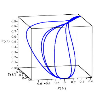
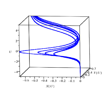
Figure 6:  

Trajectories in phase space $(x,y,z)$ for different sets of initial conditions with different values of parameter $\beta=2$ (left) and the flux in time $U=\ln a$ (right) from these figures we see that the scalar field dominated solution is the late-time attractor.

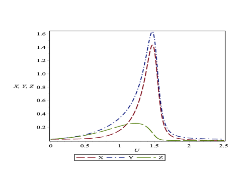
Figure 7:  

The dimensionless auxiliary variables are plotted against e-folding time $(U=\ln a)$ for $\beta=-5$

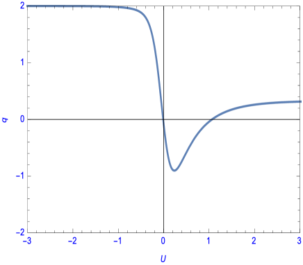
Figure 8: The plot of $q$ against $U$ for $\beta=2$

.

IV.2 When $\beta(\phi)=-\frac{1}{2x}$.

The form of the potential function in this case is given by

$V=\frac{V_{0}}{a}$

where $a$ is the scale factor. Then the autonomous system (13) reduces to

$$x^{\prime}=-3x+\frac{y^{2}}{2x}+\frac{3}{2}x\Big{(}\frac{2-z}{z}\Big{)}(z+x^{2}-y^{2})$$

$$y^{\prime}=-\frac{y}{2}+\frac{3}{2}y\Big{(}\frac{2-z}{z}\Big{)}(z+x^{2}-y^{2})$$

$$z^{\prime}=3(1-z)(z+x^{2}-y^{2})$$ (27)

The critical points of the above autonomous systems are:
$E_{6}(0,0,0)$ , $E_{7}^{\pm}(\pm 1,0,1)$ and $E_{8}^{\pm}\Big{(}\pm\frac{1}{\sqrt{6}},\sqrt{\frac{5}{6}},1\Big{)}$.

Table 7. The critical points for ASODE (27) and values of the relevant parameters

Critical point	x	y	z	Existence	${\Omega}_{\phi}~{}~{}~{}$	${\Omega}_{m}~{}~{}~{}$	${\omega}_{\phi}$
$E_{6}$	0	0	0	Always	0	0	Undefined
$E_{7}^{\pm}$	$\pm 1$	0	1	,,	1	0	1
$E_{8}^{\pm}$	$\pm\frac{1}{\sqrt{6}}$	$\sqrt{\frac{5}{6}}$	1	,,	1	0	$-\frac{2}{3}$

Table 8. Eigenvalues of the linearised matrix for the critical points of ASODE (27) and corresponding values of dimension of Stable manifold and deceleration parameters. We have defined : $B\equiv 13+\sqrt{129}$  and  $C\equiv 13-\sqrt{129}$.

Critical point	$\lambda_{1}~{}~{}~{}$	$\lambda_{2}~{}~{}~{}$	$\lambda_{3}~{}~{}~{}$	Stable manifold	q
$E_{6}$	$0~{}~{}~{}$	3	3	No stable manifold	$2$
$E_{7}^{\pm}$	$3~{}~{}~{}$	$\frac{5}{2}~{}~{}~{}$	$-6~{}~{}~{}$	1D	$2$
$E_{8}^{\pm}$	$-\frac{B}{8}~{}~{}~{}$	$-\frac{C}{8}~{}~{}~{}$	$-1~{}~{}~{}$	3D	$-\frac{1}{2}$

IV.2.1 Critical points and their properties when $\beta=-\frac{1}{2x}$:

• The critical point $E_{6}$ represents the past attractor and the cosmological implications of $E_{6}$ and $E_{1}$ are same.

• At the critical points $E_{7}^{\pm}$, the universe is completely dominated by the scalar field $(\Omega_{\phi}=1)$. As seen from Table 8 this critical points are saddle in nature. At these points expansion of the universe is also decelerated $(q=2)$.

• For the critical points $E_{8}^{\pm}$, we see that universe is dominated by the scalar field (see Table 7) and we have late-time attractor of the ASODE (27). These points are stable in the phase space and the expansion of the universe is accelerated around these points $(q=-\frac{1}{2})$. Projection of the phase trajectories on to the $xy$ plane for $\beta=-\frac{1}{2x}$ is given in FIG.(9)

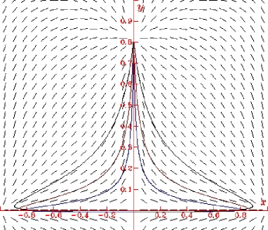
Figure 9: Projections of the phase trajectories on to the plane $(x,y)$ for $\beta=-\frac{1}{2x}$

V Classical Stability Of the Model

In previous sections we have studied local stability of the model. In order to predict the final evolution of the universe, it is also desirable to study classical stability of the model.

In cosmological perturbation theory, the speed of sound $(C_{s})$ is defined by

$$C^{2}_{s}=\frac{\frac{\partial p}{\partial U}}{\frac{\partial\rho}{\partial U}}$$ (28)

which appears as a co-efficient of the $\frac{k^{2}}{a^{2}}$ term, where $k$ is the co-moving momentum and $a$ is the usual scale factor. The model is said to be classically stable if $C^{2}_{s}$ is positive at local critical points $(x,y,z,s)$Mahata:2013oza ; pf . From cosmological point of view only those points which are locally as well as classically stable are interesting.

V.1 Scenario 1 : Exponential potential and exponential coupling function

In the Scenario 1 we have

$$C^{2}_{s}=1-\frac{\alpha~{}{\sqrt{2}}~{}{\mathrm{e}^{-\frac{b}{s}}}~{}y^{2}}{\sqrt{3~{}\mu_{0}}~{}x}$$ (29)

so for classical stability

$$\sqrt{3~{}\mu_{0}}~{}x\geq\alpha~{}{\sqrt{2}}~{}{\mathrm{e}^{-\frac{b}{s}}}~{}y^{2}$$ (30)

The local as well as classical stability criteria at critical points are summarised in Table $9$. It may be noted we can not infer about the stability of the model for the critical points $C_{1}$ , $C_{2}$ , $C_{6}$ and $C_{7}$ conclusively from above relation and for that reason we do not include these points in Table 9. From this table we can see that only $C_{4}$ and $C_{5}$ are cosmologically interesting.

Table 9. Scenario 1: Condition for classical stability at the critical point.

Critical point	x	y	z	s	Local stability	Classical stability
$C_{3}^{\pm}$	$\pm 1$	0	1	0	Unstable(saddle)	Stable
$C_{4}$	0	1	1	0	Stable	Stable(limiting)
$C_{5}$	0	$\sqrt{z}$	z	0	Stable	Stable(limiting)

V.2 Scenario 2 : Exponential potential and power law coupling parameter

In this case, the calculation for $C^{2}_{s}$ is obtained as

$$C^{2}_{s}=1-\frac{\alpha~{}{\sqrt{2}}~{}{{s}^{\frac{n}{2}}}~{}y^{2}}{\sqrt{3~{}\mu_{0}}~{}x}$$ (31)

so for classical stability

$$\sqrt{3\mu_{0}}~{}x\geq\alpha~{}{\sqrt{2}}~{}{{s}^{\frac{n}{2}}}~{}y^{2}$$ (32)

For this case, local stability and classical stability analysis for the critical points $D_{1}$-$D_{7}$ of ASODE (24) are same as Scenario 1.

V.3 When $\beta$ is constant and $\beta=-\frac{1}{2x}$

In these cases, the calculations for $C^{2}_{s}$ are same as with GR case Mahata:2013oza . We shall only present conditions for local and classical stability of the model in Table 10. Here also we can not infer about the stability of the model for the critical points $E_{1}$ , $E_{2}$ and $E_{6}$ conclusively from the relation. From this table we can see that only $E_{4}$ and $E_{5}$ are cosmologically interesting.

Table 10.: Condition for classical stability at the critical point.

Critical point	x	y	z	Local stability	Classical stability
$E_{3}^{\pm}$	$\pm 1$	0	1	Unstable(saddle)	Stable
$E_{4}$	$-\frac{\beta}{3}$	$\sqrt{1-\frac{\beta^{2}}{9}}$	1	Stable(node)	Stable if $\frac{9}{2}<\beta^{2}<9$
$E_{5}$	$-\frac{3}{2\beta}$	$\frac{3}{2\beta}$	1	Stable(node)	Stable(limiting)
$E_{7}^{\pm}$	$\pm 1$	0	1	Unstable(saddle)	Stable
$E_{8}^{\pm}$	$\pm\frac{1}{\sqrt{6}}$	$\sqrt{\frac{5}{6}}$	1	Stable(node)	Unstable

VI Discussion and conclusion

A dynamical system analysis of RS2 model of braneworld (when gravity is coupled to scalar field with a coupling function and potential) has been analysed in this work. We have taken two coupling functions (exponential and power law) corresponding to the same exponential usual potential. Performing a detailed phase-space analysis of these two scenarios, we have extracted stable solutions along with all relevant physical cosmological parameters ($\Omega_{\phi}$, $\Omega_{m}$, $\omega_{\phi}$, $q$), dimension of stable manifold and eigenvalues of the corresponding Jacobian matrices in Tables $1-8$. More or less, we get the same results for both scenarios.

Generally the dynamics of RS2 model differs from standard GR based models. In RS2 model past attractors characterise empty (Misner RS) universe in contrast to GR based result where the kinetic dominated solution is the past attractor.

While in 4D analysis we have numerically perturbed the solutions around the non-hyperbolic critical points, the linear stability analysis is enough to study the critical points in 3D. In both 4D and 3D analysis of critical points we see that it is possible to find past attractor, saddle points and future attractors under some conditions. So it fulfils our wish list and we get a complete cosmic scenario. This result is to be contrasted with similar GR based work Mahata:2013oza where we do not get complete cosmic scenario. When $\beta$=constant, we get one additional future attractor where universe will undergo decelerated expansion after accelerated expansion. This is a very interesting result which corroborates earlier results. Furthermore, we get matter scaling solution which are future attractor when $\beta$=constant. Thus, the combined effects of coupling and brane effects gives rich dynamics in contrast to interaction of dark energy in RS2 braneworld Biswas:2015zka . Here past attractor represents empty universe which is a distinctive feature of braneworld.

In addition to local stability, we have also investigated the classical stability of the model. Classical stability plays an important role in deciding final state of the universe. Only those points which are locally as well as classically stable are interesting from cosmological point of view. While in 4D analysis we see that only $C_{4}$ and $C_{5}$ are interesting and $C_{4}$ represents late time cosmic acceleration. In 3D analysis, the critical points $E_{3}^{\pm}$ and $E_{7}^{\pm}$ are classically stable but they are locally unstable in the phase space (Tables 6 and 8). Only critical points $E_{4}$ , $E_{5}$  are locally as well as classically stable and they are very interesting from cosmological point of view. For the critical points $E_{4}$ and $E_{5}$, for some restriction on the independent parameters, they will be stable points and they correspond to stable model and yields late time attractors. Here, $E_{4}$  represents late time cosmic acceleration. So we see that the present model can realise late time cosmic acceleration in all cases. It may be noted that under same coupled scalar field represented by action (3) in standard cosmology, late time acceleration can be realised only for special potential and coupling functions for which phase space becomes two dimensional. Moreover the critical points which represent late time cosmic acceleration are not classically stable Mahata:2013oza . Thus we see that coupled scalar field give rich dynamics in RS2 model in contrast to standard cosmology.

In 4D analysis we see that the critical point $C_{5}$ represents inflation whereas in 3D analysis (where potential and coupling function have special forms), early inflation is not even a critical point. It means that though RS2 braneworld favours early inflation and in this model inflation is possible for a wider class of potentials than in standard cosmology, it is not generic. Hence, a unified description of inflation and phantom (coupled scalar field) is not possible with those potential functions. It may be of considerable interest to choose $\beta$ (i.e., potential and coupling functions) such that inflation is a critical point, so we leave it for future work.

Acknowledgement:
The paper is done during a visit to IUCAA, Pune, India. The first author is thankful to IUCAA for warm hospitality and facility of doing research works. The first author would also like to thank Prof. Varun Sahni and Prof. Subenoy Chakraborty for useful discussions. Finally, the authors wish to thank the anonymous referees for helpful suggestions which lead to further improvement of this work.

References

- (1) S. J. Perlmutter, , Astrophys. J. 517, 565 (1999).
- (2) D. N. Spergel, , Astrophys J. Suppl. 148, 175 (2003) and references therein.
- (3) A. G. Riess, , Astrophys. J. 607, 665 (2004).
- (4) E. J. Copeland, M. Sami, S. Tsujikawa, Int. J. Mod. Phys. D 15, 1753 [hep-th/0603057] (2006) and references therein.
- (5) K. Bamba, S. Capozziello, S. Nojiri, S. D. Odintsov, Astrophys. Space Sci. 342 155-228, (2012).
- (6) R. Maartens, Living Rev. Relativity, 7, 7 (2004).
- (7) L. Randall, R. Sundrum, Phys. Rev. Lett. 83, 4690 (1999).
- (8) L. Randall, R. Sundrum, Phys. Rev. Lett. 83, 3370, (1999).
- (9) S. K. Srivastava, J. Dutta, Int. J. Mod. Phys. D ,18(2), 329 [arXiv:0708.4189 (gr-qc)] (2009).
- (10) R. M. Hawkins, J. E. Lidsey, Phys. Rev. D 63, 041301 (R) (2001).
- (11) G. R. Dvali, G. Gabadadze, M. Porrati, Phys. Lett. B 485, 208 [hep-th/000506] (2000).
- (12) D. Deffayet, Phys. Lett. B 502, 199 (2001).
- (13) D. Deffayet, G. R. Dvali, G. Gabadadze, Phys. Rev. D 65, 044023 [astro-ph/0105068] (2002).
- (14) R. G. Salcedo, T. Gonzalez, C. Moreno, I. Quiros, Class. Quant. Grav. 28, 105017 [arXiv:1006.1122 [gr-qc]] (2011).
- (15) J. Wainwright, G. F. R. Ellis, Dynamical Systems in Cosmology. Cambridge University Press, (1997).
- (16) A. A. Coley, Dynamical systems and cosmology. Kluwer Academic Publishers, Dordrecht Boston London, (2003).
- (17) C. G. Boehmer, N. Chan, arXiv:1409.5585 [gr-qc].
- (18) A. R. Liddle, D. H. Lyth, Cosmological inflation and Large Scale Structure. Cambridge University Press, Cambridge, England, (2003).
- (19) J. Magana, T. Matos, J. Phys. Conf. Ser. 378, 012012 (2012).
- (20) R. G. Salcedo, T. Gonzalez, Francisco A. H. Rangel, I. Quiros, D. S. Guzman, Eur. J. Phys. 32, 2, 025008 (2015).
- (21) N. Roy, N. Banerjee, Euro. Phys. J. Plus. 129, 162 (2014).
- (22) N. Roy, N. Banerjee, Annals Phys. 356, 452-466 (2015).
- (23) N. Roy, N. Banerjee, Gen. Rel. Grav. 46, 1651 (2014).
- (24) P. Rudra, R. Biswas, U. Debnath, Astrophys. Space Sci. 339, 54 (2012).
- (25) [arxiv:0907.0185]
- (26) T. Gonzalez, T. Matos, I. Quiros, A. Vazquez-Gonzalez, Phys. Lett. B 676, 161 (2009).
- (27) Y. Leyva, D. Gonzalez, T. Gonzalez, T. Matos, I. Quiros, Phys. Rev. D 80, 044026 [arXiv:0909.0281 [gr-qc]] (2009).
- (28) D. Escobar, C. R. Fadragas, G. Leon, Y. Leyva, Class. Quant. Grav. 29, 175005 (2012).
- (29) S. K. Biswas, S. Chakraborty, Gen. Rel. Grav. 47, 22 [arXiv:1502.06913 [gr-qc]](2015).
- (30) B. Gumjudpai, T. Naskar, M. Sami, S. Tsujikawa, JCAP. 0506 007, (2005).
- (31) S. Nojiri, S. D. Odintsov, Gen. Rel. Grav. 38 1285-1304, (2006).
- (32) S. Capozziello, S. Nojiri, S. D. Odintsov, Phys. Lett. B 632 597-604, (2006).
- (33) A. Sepehri, F. Rahaman, M. R. Setare, A. Pradhan, S. Capozziello, I. H. Sardar. Phys. Lett. B 747 1-8, (2015).
- (34) N. Mahata, S. Chakraborty, Gen. Rel. Grav. 46, 1721, (2014).
- (35) R. Giostri, M. V. dos santos, I. Waga, R. R. R. Reis, M. O. Calvalo, B. L. Lago, J. Cos. Astrophysics, 027, 1203 (2012).
- (36) A. D. Miller, A. D. , Astrophys. J. Lett. 524, L1 (1999).
- (37) S. Wiggins, Introduction to Applied Nonlinear Dynamical Systems and Chaos. Springer, New York Heidelberg Berlin, (1990).
- (38) S. H. Strogatz, Nonlinear Dynamics and Chaos: With Applications to Physics, Biology Chemistry and Engineering, Westview Press, Boulder, (2001).
- (39) S. C. C. Ng, N. J. Nunes, F. Rosati, Phys. Rev. D 64, 083510 [astro-ph/0107321] (2001).
- (40) R. J. Scherrer, A. A. Sen, Phys. Rev. D 77, 083515 [arXiv:0712.3450] (2008); W. Fang, Y. Li, K. Zhang, H. Q. Lu, Class. Quant. Grav. 26, 155005 [arXiv:0810.4193] (2009).
- (41) P. J. Steinhardt, L. -M. Wang, I. Zlatev, Phys. Rev. D 59, 123504 [astro-ph/9812313] (1999).
- (42) G. Leon, E. N. Saridakis, JCAP. 1303, 025 (2013).
- (43) E. J. Copeland, A. R. Liddle, D, Wands, Phys. Rev. D 57, 4686-4690 (1998).
- (44) G. Leon, E. N. Saridakis, JCAP. 0911, 006 (2009).
- (45) H. J. Schmidt,Astron. Nachr. 311, 165 (1990).
- (46) S. K. Srivastava, arXiv:0707.1376 [gr-qc].
- (47) F. Piazza, S. Tsujiikawa, JCAP 0407,004 (2004).