A user guide for Singularity

Abstract.

This is a user guide for the first version of our developed Maple library, named Singularity. The first version here is designed for the qualitative study of local real zeros of scalar smooth maps. This library will be extended for symbolic bifurcation analysis and control of different singularities including autonomous differential singular systems and local real zeros of multidimensional smooth maps. Many tools and techniques from computational algebraic geometry have been used to develop Singularity. However, we here skip any reference on how this library is developed. This package is useful for both pedagogical and research purposes. Singularity will be updated as our research progresses.

Part I How to use Singularity

In order to use Singularity in Windows and Linux platforms follow the instructions below accordingly.

I.0.1. Read option

The following command reads Singularity through which all of the commands in this user-guide will be accessible.

• Windows users: First save SingularityLibrary.mpl with an address like C:\your address\SingularityLibrary.mpl. Next, open a Maple worksheet and type

  read "C:\\your address\\SingularityLibrary.mpl".
  

• Linux users: Save SingularityLibrary.mpl with an address like /your address/SingularityLibrary.mpl. Then, open a Maple worksheet and type read "/your address/SingularityLibrary.mpl".

I.0.2. Installing Singularity on your personal computer

You can install Singularity as an additional sub-package of Maple on your personal computer through the following steps. Then, similar to built-in packages of Maple, you can use Singularity after calling with(Singularity). The latter enlists all the commands in subsections II.2 and II.3 as its output.

• Windows users: Type the following lines in a Maple worksheet

  with(LibraryTools);

  Create("C:\\Program Files\\Maple 15\\lib\\Singularity.lib");
  

  read "C:\\your address\\SingularityModule.mpl".
  

  savelib(’Singularity’,"C:\\Program Files\\Maple 15\\lib\\Singularity.lib");
  

  Then close the worksheet and open a new one.

• Linux users: Save Singularity.mla in a directory listed in the value of the predefined variable libname; see https://www.maplesoft.com/support/help/maple/view.aspx?path=libname.

Part II Introduction

In this user guide, we describe how to use the first version of our developed Maple library (named Singularity) for local bifurcation analysis of real zeros of scalar smooth maps; see [4] for the main ideas. We remark that the term singularity theory has been used in many different Mathematics disciplines with essentially different objectives and tools but yet sometimes with similar terminologies; for examples of these see [4]. For more detailed information, definitions, and related theorems in what we call here singularity theory, we refer the reader to [9, 8, 2, 3, 1, 10, 6, 7].

II.1. Verification and warning note

Singularity is able to check and verify all of its computations. However, this sometimes adds an extra computational cost. This happens mainly for finding out the correct and suitable truncation degree and computational ring. Therefore, it is beneficial to skip the extra computations when it is not necessary. For an instance of benefit, consider that you need to obtain certain results for a large family of problems arising from the same origin. Therefore, you might be able to only check a few problems and conclude about the suitable truncation degree and computational ring for the whole family. Thereby, the commands of Singularity check and verify the output results unless it requires extra computation. In this case, a warning note of not verified output or possible errors is given; in these cases, a recommendation is always provided on how to verify or circumvent the problem. Lack of warning notes always indicates that the output results have been successfully verified.

II.2. List of commands in singularity theory

The following list shows a complete list of commands from singularity theory that have so far been implemented in Singularity:

• CheckSingularity; section III.2,

• Verify; section III.3,

• Normalform; section III.4,

• UniversalUnfolding; UniversalUnfoldingPars; section III.5,

• RecognitionProblem; section III.6,

• CheckUniversal; subsection III.6.2,

• Transformation; section III.7,

• TransitionSet; subsection III.8.1.1,

• PersistentDiagram; subsection III.8.1.3,

• NonPersistent; subsection III.8.2,

• Intrinsic; section V.1,

• AlgObjects, RT, T, P, S, TangentPerp, SPerp, IntrinsicGen; section V.2.
  

II.3. Commands from computational algebraic geometry

The following enlists all implemented tools from computational algebraic geometry:

• MultMatrix; section IV.1,

• Division; section IV.2,

• StandardBasis; section IV.3,

• ColonIdeal; section IV.4,

• Normalset; section IV.5.
  

Part III Singularity theory

The terminology “singularity theory” has been used to deal with many different problems in different mathematical disciplines. Singularity theory here refers the methodologies in dealing with the qualitative behavior of local zeros

(III.0.1) $$g(x,\lambda)=0,$$

where $x\in\mathbb{R}$ is a state variable and $\lambda$ is a distinguished parameter. The cases of multi-dimensional parameter space are dealt with through the notions of unfolding. Singularity will be soon enhanced to deal with the cases of multi-dimensional state variables.

In many real life problems at certain solutions, $g(x,\lambda)$ is singular, i.e.,

$$g(x,\lambda)=g_{x}(x,\lambda)=0.$$

A singular germ $g(x,\lambda)$ subjected to smooth changes demonstrates surprising changes in the qualitative properties of the solutions, e.g., changes in the number of solutions. This phenomenon is called a bifurcation.

III.1. Qualitative properties

We define the qualitative properties as the invariance of an equivalence relation. The equivalence relation used in Singularity is contact equivalence and is defined by

(III.1.1) $$f\sim g\Leftrightarrow f(x,\lambda)=S(x,\lambda)g(X(x,\lambda),\Lambda(\lambda))$$

where $S(x,\lambda)>0$ while $(X,\Lambda)$ is locally a diffeomorphism such that $X_{x}(x,\lambda)$ and $\Lambda^{\prime}(\lambda)>0$.

III.2. Check singularity

Consider the bifurcation problem $G(x,\lambda,\alpha)=0,\alpha\in\mathbb{R}^{m},m\in\mathbb{Z}^{\geq 0}.$ The command $\verb"CheckSingularity"$ computes the singular points and their associated parameter varieties. In particular for a bifurcation problem, this command is designed to compute the varieties in the parameters space and values for the state variable $x$ where the bifurcation problem has a given singularity.

Command/the default options	Description
CheckSingularity($G$, Pars, Vars)	computes the singular points of $G$.

Here $\verb"Pars"$ represents the list of parameters $\alpha$ (but not the distinguished parameter). These parameters are usually called unfoldings, bifurcation parameters, controller inputs, or the perturbation parameters. $\verb"Vars"$ stands for the state variable $x$ and the distinguished parameter. This provides a freedom for the user to work with his/her own choice of these variables.

III.2.1. Options

• ’type’=’h$(x,\lambda)$’; where $h$ is a type of singularity. This option derives the variety in the parameter and state variable space Pars and Vars at which $G$ has the singularity of $h$-type. We remark that the singularity type $h$ is ALWAYS assumed to be in terms of the state variable $x$ and distinguished parameter $\lambda$ and their associated base point as the origin (zero). However, the state variable and distinguished parameter associated with germ $G$ are determined in the $\verb'Vars'$-list. Further, the base point of the germ $G$ can be different from the origin via the option SingularPoint described below.

• ParametricVariety; calculates the parametric variety over which $G$ attains a singularity of $h$-type.

• ’interval’; computes the parametric variety over which $G$ contains the singularity $G$ provided that Pars may only vary in the specified interval.

• ’ParsPoint’; computes the parametric variety over which $G$ acquires the singularity of $h$-type when some of the parameters in Pars receive the input values in ParsPoint option.

• ’VarsPoint’; derives the parametric variety over which $G$ contains the singularity of $h$-type when some of the variables in Vars receive the input values in VarsPoint option.

• ’plot’; plots the parametric variety over which $G$ contains the $h$-type singularity provided that Vars/Pars receive a specified input value via the option ’VarsPoint’/’ParsPoint’.

• ’SingularPoint’=’$[a,b]$’; the computations are performed when the base point is given as $a$ for the state variable and $b$ for the distinguished parameter.

• NonZero; provides the necessary non-zero conditions required for the singular germ $G$ to have a $h(x,\lambda)$-type singularity. We remark that some provided output conditions in using this option appear as equalities accompanied with some auxiliary parameters rather than nonzero conditions, i.e., inequality. However, these types of output can often be readily translated into nonzero conditions.

Example III.2.1.

The default command CheckSingularity$(x^{3}-\sin(\lambda-1)x,[x,\lambda])$ gives $(0,1)$, i.e., the germ $x^{3}-\sin(\lambda-1)x$ is singular at $(x,\lambda)=(0,1)$.

Now we provide several examples on how to use different options as follows:

1. Consider the command CheckSingularity$(x^{3}-\lambda x+\alpha+\beta x^{2},[\alpha,\beta],[x,\lambda]$, ’type’=’$x^{2}-\lambda$’, ParametricVariety). This returns

   “The bifurcation problem has singularity of ’type’=’$x^{2}-\lambda$’ for all values of parameters.”

2. The command CheckSingularity$(y^{3}-\eta y+\alpha+\beta y^{2},[\alpha,\beta],[y,\eta]$, ’type’=’$x^{3}+\lambda^{2}$’, ParametricVariety) leads to

   “ There is no singularity of this type in this bifurcation problem.”

3. The command CheckSingularity$(x^{3}+b\sin(\lambda^{2}+\alpha\exp(\lambda x)-\alpha)+\beta^{2}x\lambda,[b,\alpha,\beta],[x,\lambda]$, ’SingularPoint’=’$[0,0]$’, ’type’=’$x^{3}+\lambda^{2}$’, ParametricVariety) gives rise to

   “The bifurcation problem has singularity ’type’=’$x^{3}+\lambda^{2}$’ when $\{\alpha b+\beta^{2}=0,b\neq 0\}$.”

4. The command CheckSingularity$(z^{3}-\theta z+\alpha+\beta z^{2},[\alpha,\beta],[z,\theta]$, ’ParsPoint’=’$[\alpha=0]$’,’type’=’$x^{2}-\lambda$’, ParametricVariety) concludes

   “The bifurcation problem has singularity ’type’=’$x^{2}-\lambda$’ for all values of parameters.”

5. CheckSingularity$(x^{3}-\lambda x+\alpha+\beta x^{2},[\alpha,\beta],[x,\lambda]$, ’VarsPoint’=’$[\lambda=0]$’,’type’=’$x^{2}-\lambda$’, ParametricVariety) returns

   “The bifurcation problem has singularity ’type’=’$x^{2}-\lambda$’ when $\{4\beta^{3}+27\alpha=0\}$.”

6. CheckSingularity$(z^{3}-\theta z+\alpha+\beta z^{2},[\alpha,\beta],[z,\theta]$, ’VarsPoint’=’$[\theta=0]$’,’type’=’$x^{2}-\lambda$’, ParametricVariety, plot) gives rise to Figure 1(a).

   

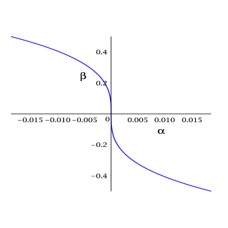
   (a)

   Figure 1. The parametric variety over which the input germ $x^{3}-\lambda x+\alpha+\beta x^{2}$ experiences the singularity $x^{2}-\lambda$.

7. CheckSingularity$(x^{3}-\lambda x+\alpha+\beta x^{2},[\alpha,\beta],[x,\lambda]$, ’interval’=’$[\alpha=[-1,1]]$’, ’type’=’$x^{2}-\lambda$’, ParametricVariety) gives

   “The bifurcation problem has singularity of ’type’=’$x^{2}-\lambda$’ for all values of parameters.”

8. CheckSingularity$(x^{3}-\lambda x+\alpha+\beta x^{2},[\alpha,\beta],[x,\lambda]$, ’type’=’$x^{2}-\lambda$’, ParametricVariety, NonZero) leads to

   “Non-zero conditions are $\{\beta\eta_{2}+1=0\}$ where the extra parameters are auxiliary.”

   We remark that the equality $\beta\eta_{2}+1=0$ for an auxiliary parameter $\eta_{2}$ is indeed translated to the inequality $\beta\neq 0$; that is a nonzero condition.

III.3. Ring and truncation degree

In this section we describe how to determine the permissible computational ring and the truncation degree. In fact, each smooth germ with a nonzero-infinite Taylor series expansion must be truncated at certain degree. Further, there are four different options in Singularity for computational rings, i.e., polynomial, fractional, formal power series and smooth germ rings, that they each can be used by commands in Singularity for bifurcation analysis of each singular germ. The command Verify(g) derives the following information about the singular germ $g$ for correct and efficient computations:

1. the permissible computational rings for the germ $g$.

2. the least permissible truncation degree $k$ for computations involving the germ $g$. In other words, the computations modulo degrees of higher than (and equal to) $k$ does not lead to error.

3. our recommended computational ring.

We are also interested in the above information for the following purpose:

• A list of germs $G$ in two variables for either division, standard basis computations, multiplication matrix, or intrinsic part of an ideal.

Command	Description
Verify($g$, Vars)	derives the permissible computational rings and permissible truncation degree.
Default upper bound for truncation	a permissible truncation degree is computed as long as it is less than or equal to $20.$

III.3.1. Options

• Ideal; Persistent; the command Verify($G$, Vars, Ideal) deals with an ideal $I$ generated by $G$, i.e., $I:=\langle G\rangle_{\mathscr{E}},$ where $G$ is a list of germs. It returns the permissible computational ring and a permissible truncation degree when the ideal $I$ is of finite codimension. Otherwise, it remarks that “the ideal is of infinite codimension.”

• Fractional; Formal; SmoothGerms; Polynomial; the command uses either the rings of fractional germs, formal power series or ring of smooth germs.

• Upper bound for truncation degree $N$; this lets the user to change the default upper bound truncation degree from $20$ to $N$.

• ’SingularPoint’=’[a, b]’; this option enables the possibility of using the values $(x,\lambda)=(a,b)$ (when $x$ stands for the state variable and $\lambda$ stands for the distinguished parameter in $g$) as the base point for the germ $g.$

Example III.3.1.

Verify($x^{3}-\sin(\lambda),[x,\lambda]$) gives

The following rings are allowed as the means of computations:

Ring of smooth germs

Ring of formal power series

Ring of fractional germs

The truncation degree must be: 4

Example III.3.2.

Verify($x^{3}-\sin(\lambda),[x,\lambda]$, 2) gives the following warning message:

“Increase the upper bound for the truncation degree!”

Example III.3.3.

Verify($[x^{4}-x\sin(\lambda),x^{3}\lambda-\lambda\sin(\lambda),3x^{4},3x^{2}\lambda],[x,\lambda],\verb"Ideal"$) gives

The following rings are allowed as means of computations:

Ring of smooth germs

Ring of formal power series

Ring of fractional germs

The truncated degree must be: 4

Example III.3.4.

Command Verify($x^{3}-\sin(\lambda)$, $[x,\lambda]$, Persistent) gives the least permissible truncation degree to be 2.

Example III.3.5.

Verify($x^{3}-\sin(\lambda-1),[x,\lambda]$, ’SingularPoint’=’$[0,1]$’) gives

The following rings are allowed as the means of computations:

Ring of smooth germs

Ring of formal power series

Ring of fractional germs

The truncation degree must be: 4

Remark III.3.6.

We remark that when a point is considered as an input in the computations, our library does not check whether it is singular or not. Thus, the user should use the command Verify or CheckSingularity in order to derive the associated singular point varieties.

III.4. Normal form

A germ $f(x,\lambda)$ is called a normal form for the singular germ $g(x,\lambda)$ when $f$ has a minimal set of monomial terms in its Taylor expansion among all contact-equivalent germs to $g$. Therefore, it is easier to analyze the solution set of $f$ while it has the same qualitative behavior as zeros of $g$ do.

Command/the default options	Description
Normalform($g$,Vars )	This function derives a normal form for $g$.
The computational ring	The default ring is the ring of fractional germs.
Verify/Warning/Suggestion	It automatically verifies if fractional germ ring is sufficient for normal form computation of the input germ $g.$ Otherwise, it writes a warning note along with a cognitive suggestion for the user.
Truncation degree	It, by default, detects the maximal degree $k$ in which $\mathcal{M}^{k+1}\subseteq\mathscr{P}(g).$ Thus, normal forms are computed modulo degrees higher than or equal to $k+1.$
Input germ	It, by default, takes the input germ $g$ as a polynomial or a smooth germ. It truncates the smooth germs modulo the degree $k+1.$

III.4.1. Options

• $k;$ specifies the degree $k$ so that computations are performed modulo degree $k+1$. When the input degree $k$ is too small for the input singular germ $g$, the computation is not reliable. Thus, an error warning note is returned to inform the user of the situation along with cognitive suggestions to circumvent the problem.

• ’SingularPoint’=’[a,b]’; this option enables the possibility of using a base point different from zero values for both the state variable and the distinguished parameter.

• Fractional, Formal, SmoothGerms; Polynomial; the command uses either the rings of fractional germs, formal power series or ring of smooth germs. When it is necessary, warning/cognitive suggestions are given accordingly.

• list; this generates a list of possible normal forms for the germ $g$. Different normal forms may only occur due to possible alternative eliminations in intermediate order terms.

Example III.4.1.

Normalform($x^{3}-\sin(\lambda),[x,\lambda]$, 10, SmoothGerms) generates

$$x^{3}-\lambda.$$

while Normalform($1-\frac{1}{1+x^{4}-\lambda^{2}},[x,\lambda]$, 10, Formal) gives rise to

$$x^{4}-\lambda^{2}.$$

Using Normalform($x^{5}+x^{3}\lambda+\sin(\lambda^{2}),[x,\lambda]$, 10, Polynomial) gives the following suggestion and warning note.

Warning: The polynomial germ ring is not suitable for normal form computations.

Suggestion: Use the command Verify to find the appropriate computational ring.

The following output might be wrong.

The germ is an infinite codimensional germ.

In fact the above statement is wrong since the high order term ideal contains

$$\mathcal{M}^{6}+\mathcal{M}^{4}\langle\lambda\rangle+\mathcal{M}\langle\lambda^{2}\rangle.$$

Now the command Verify($x^{5}+x^{3}\lambda+\sin(\lambda^{2}),[x,\lambda])$ gives rise to

Fractional germ ring; Formal power series ring; Smooth germ ring.

Thus, we use Normalform($x^{5}+x^{3}\lambda+\sin(\lambda^{2})$, $[x,\lambda]$, 10, Fractional) to obtain

$$x^{5}+x^{3}\lambda+\lambda^{2}.$$

III.5. Universal unfolding

Generally in dealing with singular problems, extra complications are experienced in the laboratory data than what are predicted by the modeling theoretical analysis. The problem here is due to modeling imperfections; natural phenomena can not be perfectly modeled by a mathematical model. In fact one usually neglects the impact of many factors like friction, pressure, and/or temperature, etc., to get a manageable mathematical model. Otherwise one will end up with a mathematical modeling problem with too many or infinite number of parameters. The imperfections around singular points may cause dramatic qualitative changes in the solution set of the model. Universal unfolding gives us a natural way to circumvent the problem of imperfections.

Definition III.5.1.

A parametric germ $G(x,\lambda,\alpha)$ for $\alpha\in\mathbb{R}^{m}$ is called an unfolding for $g(x,\lambda)$ when

$$G(x,\lambda,0)=g(x,\lambda).$$

An unfolding $G(x,\lambda,\alpha)$ for $g$ is called a versal unfolding when for each unfolding $H(x,\lambda,\beta)$ of $g(x,\lambda)$ there is a smooth germ $\alpha(\beta)$ so that $H$ is contact-equivalent to $G(x,\lambda,\alpha(\beta)).$ Roughly speaking, a versal unfolding is a parametric germ that contains a contact-equivalent copy of all small perturbations of $g(x,\lambda)$. A versal unfolding with insignificant parameters is not suitable for the bifurcation analysis. So, we are interested in a versal unfolding that has a minimum possible number of parameters, that is called universal unfolding. In other words, universal unfolding has the minimum possible number of parameters so that they accommodate all possible qualitative types that small perturbations of $g(x,\lambda)$ may experience.

Command/the default options	Description
UniversalUnfolding($g$,Vars )	This function computes a universal unfolding for $g$.
The computational ring	By default, Singularity uses the ring of fractional germs.
Verify/Warning/Suggestion	This automatically derives the least sufficient degree for truncations and also verifies if fractional germ ring is sufficient for computation. Otherwise, it writes a warning note along with guidance on the suitable rings for computations and hints at other possible capabilities of Singularity.
Degree	It, by default, detects the maximal degree $k$ in which terms of degree higher than or equal to $k+1$ can be ignored. Thus, the computations are performed modulo degree $k+1.$
Input germ	The default input germ $g$ is a polynomial or a smooth germ. For an input smooth germ, the default procedure UniversalUnfolding truncates the smooth germs modulo $k+1,$ i.e., modulo degrees higher than and equal to $k+1.$

III.5.1. Options

• normalform; A universal unfolding for normal form of $g$ is derived by this option.

• list; this function provides the list of possible universal unfoldings for $g$.

• $k$; the degree $k$ determines the truncation degree so that all computations are performed modulo $k+1.$ For low degrees of $k,$ it may derive wrong results. Thus, it gives a warning error and a suggestion for the user when $k$ must be a larger number for correct result.

• Fractional; Formal; SmoothGerms; Polynomial; this determines the computational ring. The command UniversalUnfolding gives a warning note when the user’s choice of computational ring is not suitable for computations involving the input germ $g$ and writes a suggestion to circumvent the problem.

• ’SingularPoint’=’$[a,b]$’; this provides numerical values $(a,b)$ for the state variable and the distinguished parameter, respectively.

Example III.5.2.

UniversalUnfolding$(x^{4}+4x^{3}-\lambda x,[x,\lambda],\verb"normalform",\verb"list")$ gives rise to

$$x^{3}-x\lambda+\alpha_{1}+\alpha_{2}\lambda$$

$$x^{3}-x\lambda+\alpha_{1}+\alpha_{2}x^{2}.$$

UniversalUnfolding$(6x-6\sin(x)-\lambda x,[x,\lambda],6,\verb"normalform",\verb"list",\verb"Formal")$ leads to

$$x^{3}-\lambda x+\alpha_{2}x^{2}+\alpha_{1}$$

$$x^{3}-\lambda x+\alpha_{2}\lambda+\alpha_{1}.$$

Now consider $g(x,\lambda):=x^{6}+x^{4}\lambda+\lambda^{2}.$

UniversalUnfolding$(g(x,\lambda),[x,\lambda],6,\verb"normalform",\verb"list",\verb"Polynomial")$ gives the following warning error and suggestion:

Warning: The ring of polynomial germs is not suitable for normal form computations of $g.$

Suggestion: The permissible computational ring options are Fractional, SmoothGerms and Formal.

III.5.2. Universal unfolding parameters

Consider a given parametric germ $G(x,\lambda,\alpha)$ in defenition III.5.1 when $m$ is greater than the codimension of $g.$ Therefore, it is helpful to find out all possible list of parameters which they can play the role of universal unfolding parameters. This is handled in Singularity through the following function.

Command	Description
UniversalUnfoldingPars($G$, Pars, Vars)	This function finds the list of parameters which they can play the role of universal unfolding parameters.

III.5.2.1. Options

• ’SingularPoint’=’$[a,b]$’; this provides numerical values $(a,b)$ for the state variable and the distinguished parameter, respectively.

Example III.5.3.

The command UniversalUnfoldingPars $(x^{3}-\lambda x+\sin(\alpha_{1})+\exp(\alpha_{2}\lambda+\alpha_{3})+\alpha_{4}x^{2}+\alpha_{5}\cos(x\lambda+\lambda)-1,[\alpha_{1},\alpha_{2},\alpha_{3},\alpha_{4},\alpha_{5}],[x,\lambda])$ gives

$$[\alpha_{1},\alpha_{2}],[\alpha_{1},\alpha_{4}],[\alpha_{2},\alpha_{3}],[\alpha_{2},\alpha_{5}],[\alpha_{3},\alpha_{4}],[\alpha_{4},\alpha_{5}].$$

This provides six alternative universal unfoldings for the pitchfork problem $x^{3}-\lambda x$.

III.6. Recognition problem

We describe the command RecognitionProblem on how it answers the recognition problem, that is, what kind of germs have the same normal form or universal unfolding for a given germ $g$?

III.6.1. Normal form

• Low order terms. Low order terms refer to the monomials in $\mathscr{S}(g)^{\perp}$ which do not appear in any contact-equivalent copy of $g$.

• High order terms. The ideal $\mathscr{P}(g)$ represents the space of negligible terms that are called high order terms. These terms are eliminated in normal form of $g.$

• Intermediate order terms. A monomial term are called an intermediate order term when it is neither low order nor high order term. Intermediate order terms may or may not be simplified in normal form computation of smooth germs.

The answer for the recognition problem for normal form of a germ $g$ is a list of zero and nonzero conditions for certain derivatives of a hypothetical germ $f.$ When these zero and nonzero conditions are satisfied for a given germ $f,$ the germ $f$ and $g$ are contact-equivalent. Each germ with a minimal list of monomial terms in its Taylor expansion constitutes a normal form for $g.$

III.6.2. Universal unfolding

Consider a parametric germ $G(x,\lambda,\alpha)$ and a germ $g(x,\lambda).$ Then, $G$ is usually a universal unfolding for $g$ when $G(x,\lambda,0)=g(x,\lambda)$ and certain matrix associated with $G$ has a nonzero determinant. Thus, the answer of the recognition problem for universal unfolding is actually a matrix whose components are derivatives of a hypothetical parametric germ $G$ satisfying $G(x,\lambda,0)=g(x,\lambda)$.

Command/ default	Description
RecognitionProblem($g$, Vars)	returns a list of zero and nonzero conditions on certain derivatives of a hypothetical germ $f$. A given germ $f$ is contact-equivalent to $g$ when those conditions are satisfied.
Computational ring	The default is fractional germ ring. The lack of warning notes is a confirmation that the fractional germ ring is suitable for computation.
Truncation degree	It automatically computes an optimal truncation degree $k$ and performs the remaining computations modulo degrees of higher than (but not equal to) $k$.
Verification/Warning	A warning note of possible errors is given when the computational ring is not suitable for the germ $g.$ The truncation degree is also checked and if it is not sufficiently large enough, a warning note is given. Warning notes are accompanied with cognitive suggestions to circumvent the problem.

III.6.2.1. Options

• $k$; this number represents the truncation degree.

• Computational ring: Fractional, Formal, SmoothGerms; Polynomial; the command accordingly uses either the rings of fractional germs, formal power series or smooth germs.

• UniversalUnfolding; it returns a matrix. The matrix components consists of certain derivatives of a hypothetical parametric germ $G$. Then, a parametric germ $G(x,\lambda,\alpha)$ is a universal unfolding for $g(x,\lambda)$ when $G(x,\lambda,0)=g(x,\lambda)$ and the associated matrix has a nonzero determinant.

• subs; it returns the same output as the previous option except that the derivatives of $g$ are replaced with their numeric values.

• ’SingularPoint’=’$[a,b]$’; this option refers to the base point given as $a$ for the state variable and $b$ for the distinguished parameter.

Example III.6.1.

RecognitionProblem($x^{3}+\sin(\lambda),[x,\lambda]$, 6, Formal) gives rise to

”nonzero condition=”, $[\frac{\partial}{\partial\lambda}f\neq 0,\frac{\partial^{3}}{\partial x^{3}}f\neq 0]$

”zero condition=”, $[f=0,\frac{\partial}{\partial x}f=0,\frac{\partial^{2}}{\partial x^{2}}f=0]$.

RecognitionProblem($x^{3}+\exp(\lambda^{2})-1,[x,\lambda]$, 6, UniversalUnfolding, SmoothGerms) gives rise to

$$\det\left({\begin{array}[]{ccccc}0&0&0&g_{x,x,x}(0)&g_{x,x,\lambda}(0)\\ 0&g_{\lambda,\lambda}(0)&0&g_{x,x,\lambda}(0)&g_{x,\lambda,\lambda}(0)\\ G_{\alpha_{1}}(0)&G_{\lambda,\alpha_{1}}(0)&G_{x,\alpha_{1}}(0)&G_{x,x,\alpha_{1}}(0)&G_{x,\lambda,\alpha_{1}}(0)\\ G_{\alpha_{2}}(0)&G_{\lambda,\alpha_{2}}(0)&G_{x,\alpha_{2}}(0)&G_{x,x,\alpha_{2}}(0)&G_{x,\lambda,\alpha_{2}}(0)\\ G_{\alpha_{3}}(0)&G_{\lambda,\alpha_{3}}(0)&G_{x,\alpha_{3}}(0)&G_{x,x,\alpha_{3}}(0)&G_{x,\lambda,\alpha_{3}}(0)\\ \end{array}}\right)\neq 0.$$

Now the command RecognitionProblem($x^{3}+\exp(\lambda^{2})-1,[x,\lambda]$, 6, UniversalUnfolding, Fractional,subs) returns

$$\det\left({\begin{array}[]{ccccc}0&0&0&6&0\\ 0&2&0&0&0\\ G_{\alpha_{1}}(0)&G_{\lambda,\alpha_{1}}(0)&G_{x,\alpha_{1}}(0)&G_{x,x,\alpha_{1}}(0)&G_{x,\lambda,\alpha_{1}}(0)\\ G_{\alpha_{2}}(0)&G_{\lambda,\alpha_{2}}(0)&G_{x,\alpha_{2}}(0)&G_{x,x,\alpha_{2}}(0)&G_{x,\lambda,\alpha_{2}}(0)\\ G_{\alpha_{3}}(0)&G_{\lambda,\alpha_{3}}(0)&G_{x,\alpha_{3}}(0)&G_{x,x,\alpha_{3}}(0)&G_{x,\lambda,\alpha_{3}}(0)\\ \end{array}}\right)\neq 0.$$

Let $G(x,\lambda,\alpha)$ be a parametric germ where $\alpha\in\mathbb{R}^{k}$.

Command	Description
CheckUniversal($G$, Pars, Vars)	This function checks if a parametric germ $G$ is a universal unfolding for $G(x,\lambda,0)$

• $k$; this number indicates the truncation degree.

• ’SingularPoint’=’[a,b]’; this means that the base point of singularity is given as $a$ for the state variable and $b$ for the distinguished parameter.

Example III.6.2.

CheckUniversal($x^{5}-\lambda+\alpha_{1}x+\alpha_{2}x^{2}+\alpha_{3}x^{3},[\alpha_{1},\alpha_{2},\alpha_{3}],[x,\lambda]$) gives

”Yes”

III.7. Transformations

For each two contact-equivalent germs $f$ and $g,$ there are diffeomorphic germs $(X(x,\lambda),\Lambda(\lambda))$ and smooth germ $S(x,\lambda)>0$ such that $X_{x}(x,\lambda),$ $\Lambda^{\prime}(\lambda)>0$ and $f(x,\lambda)=S(x,\lambda)g(X(x,\lambda),\Lambda(\lambda))$.

Command/option	Description
Transformation($g$, Vars)	This function computes the smooth germs $X,\Lambda,S$ transforming the germ $g$ into its normal form modulo degree $k,$ where terms of degree higher than or equal to $k$ are high order terms.
Transformation($g,f$)	This function computes suitable smooth maps $X,\Lambda,S$ for transforming the germ $g$ into $f$ modulo high order terms.

III.7.1. Options

• $k;$ this number specifies a degree $k$ so that computations are performed modulo degrees of higher or equal to $k$. When $k$ is less than the degrees of high order terms a warning note is given.

Example III.7.1.

Transformation($x^{3}+\sin(\lambda)+\exp(x^{5})-1,x^{3}+\lambda,[x,\lambda],4$) gives rise to

$$X = x+\lambda+x\lambda+\lambda^{2},\qquad\Lambda(\lambda)=\lambda,$$

$$S = 1-3x^{2}-3x\lambda-\frac{5}{6}\lambda^{2}-3x^{3}-9\lambda x^{2}-9x\lambda^{2}-3\lambda^{3}.$$

III.8. Bifurcation diagrams

Bifurcation diagram analysis of a parametric system is performed by the notion of persistent and non-persistent bifurcation diagrams. Bifurcation diagram of (III.0.1) is defined by

$$\{(x,\lambda)\mid g(x,\lambda,\alpha)=0\}.$$

A bifurcation diagram is called persistent when the bifurcation diagrams subjected to small perturbations in parameter space remain self contact-equivalent.

III.8.1. Persistent bifurcation diagram classification and transition set

The classification of persistent bifurcation diagrams are performed by the notion of transition sets. In fact, a subset of parameter space is called transition set when the associated bifurcation diagrams are non-persistent. Transition set is denoted by $\Sigma$ and is usually a hypersurface of codimension one for germs of finite codimension. Then, one choice from each connected components of the complement of the transition set $\Sigma$ makes a complete persistent bifurcation diagram classification of a given parametric germ. This provides a comprehensive insight into the persistent zero solutions of a parametric germ.

III.8.1.1. Transition set

The parameters associated with non-persistent bifurcation diagrams are split into three categories: bifurcation, hysteresis, and double limit point. These are defined and denoted by

$$\mathscr{B} = \{\alpha\in\mathbb{R}^{p}\mid G=G_{x}=G_{\lambda}=0\hbox{ at }(x,\lambda,\alpha)\hbox{ for some }(x,\lambda)\in\mathbb{R}\times\mathbb{R}\},$$

$$\mathscr{H} = \{\alpha\in\mathbb{R}^{p}\mid G=G_{x}=G_{xx}=0\hbox{ at }(x,\lambda,\alpha)\hbox{ for some }(x,\lambda)\in\mathbb{R}\times\mathbb{R}\},$$

$$\mathscr{D} = \{\alpha\in\mathbb{R}^{p}\mid\exists(x_{1},x_{2},\lambda)\in\mathbb{R}\times\mathbb{R}\times\mathbb{R}\hbox{ so that }G=G_{x}=0\hbox{ at }(x_{1},\lambda,\alpha)\hbox{ and }$$

$$\;(x_{1},\lambda,\alpha)\}.$$

The transition set $\Sigma$ is now given by $\Sigma:=\mathscr{B}\cup\mathscr{H}\cup\mathscr{D}$. Suppose that $H$ is a singular parametric germ.

Command/the default options	Description
TransitionSet($H$, Pars, Vars)	This function estimates the transition set in terms of parameters of $H.$ The default is to eliminate $x$ and $\lambda$ variables from the equations given by $\mathscr{B},\mathscr{H},\mathscr{D}$.
Truncation degree	For non-polynomial input germs, by default, it automatically computes a suitable truncation degree $k$ and truncates the input germ at degree $k$, i.e., preserving degrees of less than and equal to $k$.

III.8.1.2. Options

• Pars:=$[\alpha_{1},\alpha_{2},\ldots,\alpha_{p}]$; this hints to derive the transition set in terms of these variables while the attempts are best made to eliminate the rest of variables from the equations (as many as possible).

• plot; this function plots/animates transition set in parameter space.

• $\alpha_{i}$; When codimension is more than or equal to three 3, some parameters $\alpha_{3},\alpha_{4},\ldots$ will be taken as fixed by default. This option refines the plot/animate option by allowing to change the fixed parameters to $\alpha_{i}.$

• $k$; determines the truncation degree. The user may use the command Verify to find an appropriate degree $k.$

• ’SingularPoint’=’[a,b]’; the computations are performed for the base point given as $a$ for the state variable and $b$ for its distinguished parameter.

Example III.8.1.

Here, we bring two examples from [7, Page 206].

TransitionSet($x^{4}-\lambda x+\alpha_{1}+\alpha_{2}\lambda+\alpha_{3}x^{2},[\alpha_{1},\alpha_{2},\alpha_{3}],[x,\lambda]$) gives rise to

$$\mathscr{B} := \{(\alpha_{1},\alpha_{2},\alpha_{3})\,|\,\alpha_{2}^{4}+\alpha_{2}^{2}\alpha_{3}+\alpha_{1}=0\},$$

$$\mathscr{H} := \{(\alpha_{1},\alpha_{2},\alpha_{3})\,|\,128\alpha_{2}^{2}\alpha_{3}^{3}+3\alpha_{3}^{4}+72\alpha_{1}\alpha_{3}^{2}+432\alpha_{1}^{2}=0\},$$

$$\mathscr{D} := \{(\alpha_{1},\alpha_{2},\alpha_{3})\,|\,-\alpha_{3}^{2}+4\alpha_{1}=0,\,\alpha_{3}\leq 0\}.$$

TransitionSet($x^{5}-\lambda+\alpha_{1}x+\alpha_{2}x^{2}+\alpha_{3}x^{3},[\alpha_{1},\alpha_{2},\alpha_{3}],[x,\lambda]$) derives

$$\mathscr{B} := \emptyset,$$

$$\mathscr{H} := \{(\alpha_{1},\alpha_{2},\alpha_{3})\,|\,-81\alpha_{1}\alpha_{3}^{4}+27\alpha_{2}^{2}\alpha_{3}^{3}+360\alpha_{1}^{2}\alpha_{3}^{2}$$

$$-540\alpha_{1}\alpha_{2}^{2}\alpha_{3}+135\alpha_{2}^{4}-400\alpha_{1}^{3}=0\},$$

$$\mathscr{D} := \{(\alpha_{1},\alpha_{2},\alpha_{3})\,|\,-16\alpha_{3}^{6}+224\alpha_{1}\alpha_{3}^{4}-88\alpha_{2}^{2}\alpha_{3}^{3}$$

$$-1040\alpha_{1}^{2}\alpha_{3}^{2}+360\alpha_{1}\alpha_{2}^{2}\alpha_{3}+135\alpha_{2}^{4}+1600\alpha_{1}^{3}=0\}.$$

Example III.8.2.

TransitionSet($x^{3}+\sin(\lambda x)+\alpha_{1}+\alpha_{2}x^{2},[\alpha_{1},\alpha_{2}],[x,\lambda],5$, plot) generates Figure 4(a).

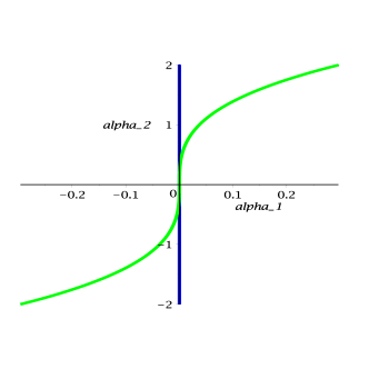
(a)

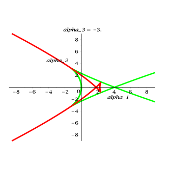
(b)

Figure 2. Blue color is for bifurcation $\mathscr{B}$, green stands for hysteresis $\mathscr{H}$ while the red color depicts transition set associated with double limit point $\mathscr{D}$.

TransitionSet($x^{5}-\lambda+\alpha_{1}x+\alpha_{2}x^{2}+\alpha_{3}x^{3},[\alpha_{1},\alpha_{2},\alpha_{3}],[x,\lambda],\verb"plot"$) creates an animation ending at Figure 2(b).

III.8.1.3. Persistent bifurcation diagrams

The command $\verb"PersistentDiagram"$ follows the following table.

Command/the default options	Description
PersistentDiagram($H$, Vars)	this function plots/animates bifurcation diagrams in $x-\lambda$ plane by passing through the parameter space. The default path is a circle around the singular point and it may include at most two parameters.

III.8.1.4. Options

• $\alpha_{i}$; for parameter space of dimension more than two, it chooses three values for $\alpha_{i}$, i.e., a negative, zero and a positive value for $\alpha_{i}$. Then, it plots/animates bifurcation diagrams in $x-\lambda$ plane by passing (circular path by default) through parameter space for fixed parameter $\alpha_{i}$.

• $f(\zeta),g(\zeta)$; this function animates bifurcation diagrams in $x-\lambda$ plane by passing through the given path ($f(\zeta),g(\zeta)$).

• ShortList; IntermediateList; CompleteList; either of these generates a list of points associated persistent bifurcation diagrams.

• plot; this option plots the persistent bifurcation diagrams associated with parameter points output of the previous option, i.e., ShortList; IntermediateList; CompleteList.

• $k$; determines the truncation degree of the germ $H.$

• ’values’=’$[\alpha_{1}=a_{1},\ldots,\alpha_{m}=a_{m}]$’; plots persistent diagrams where parameters $\alpha_{i}$ receive the values $a_{i}$ for $i=1,\ldots,m$.

• ’IntervalPlot’=’$[x=x_{0}..x_{1},\lambda=\lambda_{0}..\lambda_{1}]$’; plots persistent diagrams over the vertical and horizontal axes $x$ and $\lambda$ with the ranges $x_{0}..x_{1}$ and $\lambda_{0}..\lambda_{1}$, respectively.

Example III.8.3.

Now we present how the command PersistentDiagram works.

PersistentDiagram($x^{5}-\lambda+\alpha_{1}x+\alpha_{2}x^{2}+\alpha_{3}x^{3}$, $[x,\lambda]$ , plot, CompleteList) generates a list from which the list of inequivalent bifurcation diagrams are chosen in Figure 3.

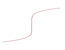
(a)

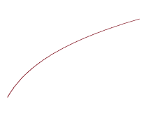
(b)

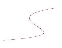
(c)

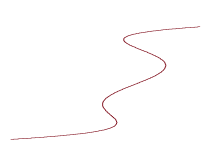
(d)

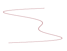
(e)

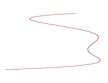
(f)

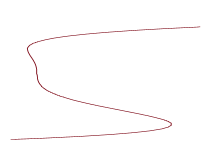
(g)

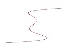
(h)

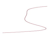
(i)

Figure 3. Persistent bifurcation diagrams associated with $x^{5}-\lambda+\alpha_{1}x+\alpha_{2}x^{2}+\alpha_{3}x^{3}$.

III.8.2. Singular boundary conditions

Extra sources of non-persistent is caused by singular boundary conditions of a parametric scalar map restricted to a bounded domain. Let $W\subset\mathbb{R}^{m}$ be a closed disk and $U,L\subset\mathbb{R}$ be two closed intervals. Next, consider

$$F(x,\lambda,\alpha)=0$$

where $\alpha\in W$ and $(x,\lambda)\in U\times L$; see [7, Pages 154-158]. The new non-persistent sources are defined by

$$\mathscr{L}_{C} := \{\alpha\in W\mid F(x,\lambda,\alpha)=0\hbox{ for some }(x,\lambda)\in\partial U\times\partial L\},$$

$$\mathscr{L}_{SH} := \{\alpha\in W\mid F=F_{x}=0\hbox{ for some }(x,\lambda)\in\partial U\times L\},$$

$$\mathscr{L}_{SV} := \{\alpha\in W\mid F=F_{x}=0\hbox{ for some }(x,\lambda)\in U\times\partial L\},$$

$$\mathscr{L}_{T} := \{\alpha\in W\mid F=F_{\lambda}=0\hbox{ for some }(x,\lambda)\in\partial U\times L\},$$

$$\mathscr{G}_{1} := \{\alpha\in W\mid F=0\hbox{ at }(x_{0},\lambda,\alpha)\hbox{ for some }(x_{0},\lambda)\in\partial U\times L,$$

$$x_{0}\neq x\hbox{ and }F=F_{x}=0\hbox{ at }(x,\lambda,\alpha)\hbox{ for some }(x,\lambda)\in U\times L\},$$

$$\mathscr{G}_{2} := \{\alpha\in W\mid\exists(x_{1},\lambda),(x_{2},\lambda)\in\partial U\times L,x_{1}\neq x_{2}\hbox{ s.t }F=0\hbox{ at }$$

$$(x_{i},\lambda,\alpha)\hbox{ for }i=1,2\},$$

$$\mathscr{L_{B}} := \{\alpha\in W\mid F=F_{x}=F_{\lambda}=0\hbox{ at }(x,\lambda,\alpha)\hbox{ for some }$$

$$(x,\lambda)\in U\times L\},$$

$$\mathscr{L_{H}} := \{\alpha\in W\mid F=F_{x}=F_{xx}=0\hbox{ at }(x,\lambda,\alpha)\hbox{ for some }$$

$$(x,\lambda)\in U\times L\},$$

$$\mathscr{G}_{D} := \{\alpha\in W\mid\exists(x_{1},\lambda),(x_{2},\lambda)\in U\times L,x_{1}\neq x_{2}\hbox{ s.t }F=F_{x}=0\hbox{ at }$$

$$(x_{i},\lambda,\alpha)\hbox{ for }i=1,2\}.$$

In this case, the transition set is given by $\Sigma:=\mathscr{L}\cup\mathscr{G}$, here

$$\mathscr{L} := \mathscr{L_{B}}\cup\mathscr{L_{H}}\cup\mathscr{L}_{C}\cup\mathscr{L}_{SH}\cup\mathscr{L}_{SV}\cup\mathscr{L}_{T},$$

$$\mathscr{G} := \mathscr{G}_{D}\cup\mathscr{G}_{1}\cup\mathscr{G}_{2}.$$

For a finite codimension singular germ, $\Sigma$ is a hypersurface of codimension one and each two choices from a connected component in the complement of $\Sigma$ are contact-equivalent. Therefore, we can classify the persistent bifurcation diagrams by merely choosing one representative parameter from each components of the complement set of $\Sigma$ and plotting the associated bifurcation diagrams. The command NonPersistent is designed for this purpose.

Command/default option	Description
NonPersistent($F$, $\alpha$, Vars, $U$, $L$)	This function computes transition set for $F$ where bifurcation diagrams are limited on $U\times L$. Here, $U$ and $L$ are only taken as closed intervals. Further, it plots the transition set.
Box of figures	It plots transition set in $[-1,1]\times[-1,1]$ by default.

III.8.2.1. Options

• $V,W$; this option enforces that the computed transition set is plotted in $V\times W$ instead of the default square $[-1,1]\times[-1,1]$.

• Vertical (Horizontal is also similar); this assumes that the boundary conditions is $U\times\mathbb{R},$ i.e., there is only singular boundary conditions on vertical boundary lines.

Example III.8.4.

NonPersistent($x^{4}-\lambda x+\alpha_{1}x+\alpha_{2}\lambda+\alpha_{3}x^{2},[\alpha_{1},\alpha_{2},\alpha_{3}],[x,\lambda],[-2,2],[1,3]$) gives rise to

$$\mathscr{L}_{C} = \{(\alpha_{1},\alpha_{2},\alpha_{3})\,|\,\alpha_{1}+18+4\alpha_{3}+\alpha_{2}=0,\alpha_{1}+22+4\alpha_{3}+3\alpha_{2}=0,$$

$$\alpha_{1}+14+4\alpha_{3}+\alpha_{2}=0,\alpha_{1}+10+4\alpha_{3}+3\alpha_{2}=0\},$$

$$\mathscr{L}_{SH} = \{(\alpha_{1},\alpha_{2},\alpha_{3})\,|\,4\alpha_{2}\alpha_{3}-\alpha_{1}+32\alpha_{2}+4\alpha_{3}+48=0,4\alpha_{2}\alpha_{3}+\alpha_{1}$$

$$+32\alpha_{2}-4\alpha_{3}-48=0\},$$

$$\mathscr{L}_{SV} = \{(\alpha_{1},\alpha_{2},\alpha_{3})\,|\,16\alpha_{1}\alpha_{3}^{4}+16\alpha_{2}\alpha_{3}^{4}-128\alpha_{1}^{2}\alpha_{3}^{2}-256\alpha_{1}\alpha_{2}\alpha_{3}^{2}-128\alpha_{2}^{2}\alpha_{3}^{2}$$

$$+256\alpha_{1}^{3}+768\alpha_{1}^{2}\alpha_{2}+768\alpha_{1}\alpha_{2}^{2}+256\alpha_{2}^{3}-4\alpha_{3}^{3}+144\alpha_{1}\alpha_{3}+144\alpha_{2}\alpha_{3}-27=0,$$

$$16\alpha_{1}\alpha_{3}^{4}+48\alpha_{2}\alpha_{3}^{4}-128\alpha_{1}^{2}\alpha_{3}^{2}-768\alpha_{1}\alpha_{2}\alpha_{3}^{2}-1152\alpha_{2}^{2}\alpha_{3}^{2}+256\alpha_{1}^{3}+2304\alpha_{1}^{2}\alpha_{2}$$

$$+6912\alpha_{1}\alpha_{2}^{2}+6912\alpha_{2}^{3}-36\alpha_{3}^{3}+1296\alpha_{1}\alpha_{3}+3888\alpha_{2}\alpha_{3}-2187=0\},$$

$$\mathscr{L}_{T} = \{(\alpha_{1},\alpha_{2},\alpha_{3})\,|\,\alpha_{2}+2=0,4\alpha_{3}+16+\alpha_{1}=0,\alpha_{2}-2=0,4\alpha_{3}+16+\alpha_{1}=0\},$$

$$\mathscr{G}_{1} = \{(\alpha_{1},\alpha_{2},\alpha_{3})\,|\,4\alpha_{2}^{2}\alpha_{3}^{3}+80\alpha_{2}^{2}\alpha_{3}^{2}+16\alpha_{2}\alpha_{3}^{3}-72\alpha_{1}\alpha_{2}\alpha_{3}+512\alpha_{2}^{2}\alpha_{3}$$

$$+32\alpha_{2}\alpha_{3}^{2}+16\alpha_{3}^{3}+27\alpha_{1}^{2}-320\alpha_{1}\alpha_{2}+72\alpha_{1}\alpha_{3}+1024\alpha_{2}^{2}-384\alpha_{2}\alpha_{3}$$

$$+176\alpha_{3}^{2}+224\alpha_{1}-1024\alpha_{2}+640\alpha_{3}+768,4\alpha_{2}^{2}\alpha_{3}^{3}+80\alpha_{2}^{2}\alpha_{3}^{2}-16\alpha_{2}\alpha_{3}^{3}$$

$$+72\alpha_{1}\alpha_{2}\alpha_{3}+512\alpha_{2}^{2}\alpha_{3}-32\alpha_{2}\alpha_{3}^{2}+16\alpha_{3}^{3}+27\alpha_{1}^{2}+320\alpha_{1}\alpha_{2}+72\alpha_{1}\alpha_{3}$$

$$+1024\alpha_{2}^{2}+384\alpha_{2}\alpha_{3}+176\alpha_{3}^{2}+224\alpha_{1}+1024\alpha_{2}+640\alpha_{3}+768=0\},$$

$$\mathscr{G}_{2} = \{(\alpha_{1},\alpha_{2},\alpha_{3})\,|\,4\alpha_{3}+16+\alpha_{1}=0\},$$

$$\mathscr{L_{B}} = \{(\alpha_{1},\alpha_{2},\alpha_{3})\,|\,\alpha_{2}^{4}+\alpha_{2}^{2}\alpha_{3}+\alpha_{1}=0\},$$

$$\mathscr{L_{H}} = \{(\alpha_{1},\alpha_{2},\alpha_{3})\,|\,128\alpha_{2}^{2}\alpha_{3}^{3}+3\alpha_{3}^{4}+72\alpha_{1}\alpha_{3}^{2}+432\alpha_{1}^{2}=0\},$$

$$\mathscr{G}_{D} = \{(\alpha_{1},\alpha_{2},\alpha_{3})\,|\,\alpha_{3}^{2}-4\alpha_{1}=0\},$$

and generates Figure 4.

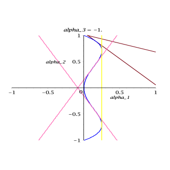
(a)

Figure 4. Transition set

Part IV Tools from algebraic geometry

In this section we describe how to compute some tools from computational algebraic geometry; see [4] for more information.

IV.1. Multiplication Matrix

Let $\mathcal{R}$ be either of the rings of germs $\mathscr{E},$ $\mathbb{R}[[x,\lambda]],$ $\mathbb{R}[x,\lambda]_{\langle x,\lambda\rangle}$ or $R[x,\lambda]$; see [4]. Now we describe how to compute the multiplication Matrix defined by

(IV.1.1) $$\varphi_{u,J}:\frac{\mathcal{R}}{J}\rightarrow\frac{\mathcal{R}}{J},\quad\varphi_{u,J}(f+J):=uf+J,$$

where $J$ is an ideal generated by a finite set $A\subset\mathcal{R},$ i.e., $J:=\langle A\rangle_{\mathcal{R}}$, and $u$ is a monomial; also see [4, Equation 3.4].

Command/option	Description
MultMatrix($A$, $u$, Vars)	This function derives $\varphi_{u,J}$ where $u$ is a monomial, $\varphi_{u,J}$ is defined by Equation (IV.1.1).
Default computational ring	the fractional germ ring.
Truncation degree	When the input set of germs $A$ only includes polynomials, MultMatrix($A$, $u$, Vars) does not need truncation degree. However, for non-polynomial input germs, a truncation degree $k$ needs to be included.

IV.1.1. Options

• $k$; determines the truncation degree. The user is advised to use the command Verify to find an appropriate truncation degree $k.$

• Computational ring: Fractional, Formal, SmoothGerms; Polynomial; the command uses either the rings of fractional germs, formal power series or ring of smooth germs. The command Verify is an appropriate tool to find/verify the appropriate computational ring.

Example IV.1.1.

The command MultMatrix($[x^{6}+\frac{12}{27}x^{1}0\lambda^{9},\frac{5}{3}x^{5}+\lambda\sin(x^{3}),\lambda^{2}-\frac{2}{3}(1-\exp(x^{5}))],x,[x,\lambda],6,\verb"Formal"$) gives rise to

$$\left({\begin{array}[]{ccccccccc}0&0&0&0&0&0&0&0&0\\ 0&0&0&0&0&0&0&0&0\\ 1&0&0&0&0&0&0&0&0\\ 0&0&1&0&0&0&0&0&0\\ 0&0&0&1&0&0&0&0&0\\ 0&0&0&0&1&0&0&0&0\\ 0&0&0&0&0&1&0&0&-\frac{5}{3}\\ 0&1&0&0&0&0&0&0&0\\ 0&0&0&0&0&0&0&1&0\\ \end{array}}\right).$$

IV.2. Divisions of germs

The following table describes how to use the command Division to divide a germ $g$ by a set of germs $G:=\{f_{i}|i=1,\ldots n\}$ where all these germs are in terms of the variables in Vars. Note that the ordering in the list of variables Vars is important and determines how anti-lexicographical ordering is defined.

Command	Description
Division($g$, $G$, Vars)	This divides the germ $g$ by the germs in $G$ using anti-lexicographical ordering.

IV.2.1. Options

• Formal; SmoothGerms; Polynomial; Fractional; this determines the computational germ ring. In order to verify/check the computational ring for the division, one is advised to use the command Verify(G, Ideal, Vars) and find the permissible computational ring.

• $k$; this option enforces the computations modulo degrees higher than or equal to $k+1.$ The command Verify(G, Ideal, Vars) also suggests an optimal permissible truncation degree $k$.

Example IV.2.1.

For an example we use Division($\sin(x^{7})-1,[x^{5}+x^{6}\exp(\lambda),xy^{3}-\frac{2}{7}x\lambda^{6}-x^{7},\lambda\cos(x^{7})],$ $[x,\lambda],8,\verb"SmoothGerms"$). This returns

$$-1$$

as the remainder of

$$\sin(x^{7})-1$$

divided by

$$\{x^{5}+x^{6}\exp(\lambda),xy^{3}-\frac{2}{7}x\lambda^{6}-x^{7},\lambda\cos(x^{7})\}$$

using the anti-lexicographical ordering with $x\succ\lambda$.

IV.3. Standard basis

Now we describe how to compute a standard basis for a set of germs in either of the following local rings: fractional germs $\mathbb{R}[x,\lambda]_{\langle x,\lambda\rangle}$, formal power series $\mathbb{R}[[x,\lambda]],$ and ring of smooth germs $\mathscr{E}$; see [4]. The command StandardBasis follows the table and options described below. Note that Vars denotes an order list of variables and the germs in $G$ are in terms of the variables in Vars. The anti-lexicographical ordering is here used while it is determined by the ordering of variables in Vars.

Command	Description
StandardBasis($G$, Vars)	computes the standard basis of the polynomial germs in $G$ in the fractional germ ring.
Default computational ring	fractional germ ring.
Default input	the default germs in $G$ must be polynomial germs. For the cases of non-polynomials, it needs a truncation degree $k.$

IV.3.1. Options

• $k$; this determines the truncation degree.

• Consider the cases that the option $k$ is used. A warning note is given when the truncation degree $k$ is not sufficiently high to guarantee that the output is correct. A warning note is given like “The truncation degree is not sufficiently high and thus, the following results might be wrong.” In this case, for an appropriate truncation degree $l$ is given.

• Formal; SmoothGerms; Fractional; this determines the computational germ ring and computes the standard basis accordingly.

Example IV.3.1.

For an example, the command StandardBasis($[x^{5}+x^{2}\sin(\lambda+x)+\lambda^{2},x^{3}\lambda^{2}+\cos(\lambda)x,\lambda^{6}+x^{4}-\lambda x],[x,\lambda],7,\verb"SmoothGerms"$) computes the standard basis of the set of germs

$$\{x^{5}+x^{2}\sin(\lambda+x)+\lambda^{2},x^{3}\lambda^{2}+\cos(\lambda)x,\lambda^{6}+x^{4}-\lambda x\}$$

as $\{x,\lambda^{2}\}.$

IV.4. Colon ideals

The colon ideal $I:\langle g\rangle$ refers to the ideal defined by

$$I:\langle g\rangle_{\mathscr{E}}=\{f\in\mathscr{E}:f\langle g\rangle_{\mathscr{E}}\subseteq I\}.$$

Using the arguments on [4, Page 22], we have $I:\langle g\rangle_{\mathscr{E}}=\langle\frac{h_{i}}{g}|i=1,\ldots,n\rangle_{\mathscr{E}},$ where $h_{1},h_{2},\ldots,h_{n}$ is a standard basis for the ideal $I\cap\langle g\rangle_{\mathbb{R}[x,\lambda]}.$ The command ColonIdeal follows this.

Command	Description
ColonIdeal($I$, $g$)	computes the colon ideal $I:g$ for $g$ in $\mathscr{E}$.

Example IV.4.1.

ColonIdeal($[x^{7}+\lambda x^{3}-\lambda^{2}x,\lambda x^{6}+\lambda^{2}x^{2}-\lambda^{3},x^{3}\lambda+x],\lambda$) leads to the ideal generated by

$$[x(\lambda x^{2}+1),\lambda^{2}x^{2}-x^{4}-\lambda^{3},\lambda^{4}+\lambda^{2}-x^{2},x(x^{4}+\lambda^{3}+\lambda)].$$

IV.5. Complement spaces

For computing universal unfolding of a singular germ $g$, we need to compute a basis for a complement vector space for the tangent space $T(g)$ associated with $g.$ This is equivalent to computing a basis for the quotient space $\mathscr{E}/T(g).$ More generally, the command Normalset($I$) computes a monomial basis for $\mathscr{E}/I$, when $I$ is either an ideal or a vector space with finite codimension in the local ring $\mathscr{E}$.

Command	Description
Normalset($A$)	computes a monomial basis for $\mathscr{E}/I$, when $A$ is a list of germs generating an ideal $I:=\langle A\rangle$.

Example IV.5.1.

For example the command Normalset($[x^{6}+\lambda x^{4}+\lambda^{2}x,\lambda x^{5}+\lambda^{2}x^{3}+\lambda^{3},5x^{6}+3\lambda x^{4},5\lambda x^{4}+3\lambda^{2}x^{2},-3x^{7}-3\lambda x^{5}-\frac{25}{3}x^{6}]$) returns

$$[1,\lambda,x,\lambda^{2},x^{2},x^{3},x^{4},x^{5},\lambda x,\lambda x^{3},x^{2}\lambda]$$

as a list of monomials for the complement of $I$ in $\mathscr{E}.$

Part V Technical objects in singularity theory

A user who is not interested in technical details and their commands may simply skip this section.

V.1. Intrinsic ideals

In this section we describe how to compute the intrinsic part of an ideal or a vector space. Let $A$ and $B$ be two lists indicating the generators of an ideal and a vector space, respectively. We intend to compute the maximal intrinsic ideal contained in $\langle A\rangle_{\mathscr{E}}+\langle A\rangle_{\mathbb{R}}.$

Command/option	Description
Intrinsic($A$, Vars)	computes intrinsic part of the ideal generated by $A$. It remarks when the ideal is of infinite codimension.
Intrinsic($A,B$, Vars)	computes intrinsic part of a vector space given by $\langle A\rangle_{\mathscr{E}}+\langle B\rangle_{\mathbb{R}}.$ It remarks when the vector space is of infinite codimension.
Computational ring	The default computational ring is the ring of fractional germs.
Verify/Warning/Suggestion	By default, Intrinsic checks and verifies whether the fractional germ ring is sufficient for computation of the intrinsic part of the ideal or vector space spanned by $A$ (and $B$). If fractional germ ring is not sufficient, it gives a warning note of possible errors and a suggestion to circumvent the problem. Intrinsic remarks when the problem might be of infinite codimension. Despite possible warning errors, Intrinsic computes the intrinsic part using the fractional germ ring.

V.1.1. Options

• $k$; this option enforces that the computations are performed modulo degree $k.$

• Formal; SmoothGerms; Polynomial; Fractional; this determines the computational germ ring. It checks and verifies the computations. It gives warning notes of possible errors and alternative suggestions when it finds them necessary.

Example V.1.1.

For an example Intrinsic$([x^{3}\lambda+\lambda^{2},3x^{3}\lambda,3x^{2}\lambda^{2}],$ $[x,\lambda]$, $\verb"InfCodim"$, $\verb"Fractional")$ leads to

$$M^{3}\langle\lambda\rangle+\langle\lambda^{2}\rangle.$$

As for a second example Intrinsic($[x^{5}+\lambda x^{3}+\lambda^{2},5x^{5}+3x^{3}\lambda,5x^{4}\lambda+3x^{2}\lambda^{2}],[\lambda x^{3}+2\lambda^{2},x^{3}+2\lambda,x^{4}+\frac{3}{5}\lambda x^{2},\lambda^{2},x^{5}],[x,\lambda]$) results in

$$M^{5}+M^{3}\langle\lambda\rangle+\langle\lambda^{2}\rangle.$$

V.2. Algebraic objects

Singularity theory defines and uses many algebraic objects in the bifurcation analysis of zeros of smooth germs. These include restricted tangent space $RT$, tangent space $T$, high order term ideal $\mathscr{P}$, smallest intrinsic ideal associated with a singular germ $\mathscr{S}$, a basis for complement of the tangent space $\mathscr{E}/T$, and low order terms $\mathscr{S}^{\perp}$; see [4, 7]. These can be computed in Singularity using the command AlgObjects as well as the individual commands RT, T, P, and TangentPerp. The individual commands RT, T, and P have the same default and non-default options as AlgObjects has as follows.

Command/option	Description
AlgObjects($g$, Vars)	This function computes $RT$, $T$, $\mathscr{P}$, $\mathscr{E}/T$, $\mathscr{S}$, $\mathscr{S}^{\perp}$ and intrinsic generators of $\mathscr{S}$ for given $g$.
RT(g, Vars)	This derives the restricted tangent space associated with a scalar smooth germ $g$.
T(g, Vars)	This command provides a nice representation of the tangent space associated with the singular smooth germ $g.$ The representation uses intrinsic ideal representation as for the intrinsic part of $T(g)$.
p(g, Vars)	This computes the high order term ideal associated with the germ $g$.
TangentPerp(g, Vars)	This first computes $T(g)$, i.e., the tangent space of the germ $g,$ and then returns a monomial basis for the complement space of $T(g)$.
S(g, Vars)	Computes the smallest intrinsic ideal containing the germ $g$.
SPerp(g, Vars)	This derives a set of monomials of low order terms for the germ $g$.
IntrinsicGen(g, Vars)	This derives the intrinsic generators of $\mathscr{S}(g)$ that determine the nonzero conditions for recognition problem for normal forms.
Computational ring	The default computational ring is the ring of fractional germs.
Default degree $k$	For non-polynomial input germs, it computes the least degree $k$ so that truncations at degree $k$ is permissible. Next, the germ $g$ is truncated and all algebraic objects are computed modulo degrees higher than or equal to $k+1$.

V.2.1. Options

• $k$; this option enforces the computations modulo degree $k+1.$

• Formal; SmoothGerms; Polynomial; Fractional; this determines the computational germ ring. It checks and verifies/gives warning notes of possible errors.

Example V.2.1.

Now we present three examples of singular germs of high codimension; see and compare these examples with the examples in [8, Page 4]. For example we consider a codimension 10 singularity and use AlgObjects($x^{5}+x^{3}\lambda^{2}+\lambda^{3},[x,\lambda],\verb"Fractional"$). It gives

$$\mathscr{P} = M^{6}+M\langle\lambda^{3}\rangle,$$

$$RT = M^{6}+M\langle\lambda^{3}\rangle+\langle x^{4}\lambda,3\lambda^{2}x^{3}+5x^{5},\lambda^{2}x^{3}+x^{5}+\lambda^{3}\rangle,$$

$$T = M^{5}+\langle\lambda^{3}\rangle+\{\frac{3}{5}\lambda^{2}x^{2}+x^{4},x^{3}\lambda+\frac{3}{2}\lambda^{2}\},$$

$$\mathscr{E}/T = \{1,\lambda,x,\lambda^{2},x^{2},x^{3},\lambda x^{2},\lambda^{2}x,\lambda^{2}x^{2},x\lambda\},$$

$$\mathscr{S} = M^{5}+\langle\lambda^{3}\rangle,$$

$$\mathscr{S}^{\perp} = \{1,\lambda,x,\lambda^{2},x^{2},x^{3},x^{4},\lambda x^{2},\lambda^{2}x,\lambda^{2}x^{2},x\lambda,x^{3}\lambda\},$$

intrinsic generators $$= \{x^{5},\lambda^{3}\}.$$

A codimension 20 singularity: TangentPerp($x^{8}+\sin(\lambda^{3}),[x,\lambda],9$) derives the following

$$T = M^{9}+\langle\lambda^{3}\rangle+\{x^{7},x^{8},\lambda x^{7},-2\lambda^{2}\},$$

TangentPerp $$= \{1,\lambda,x,x^{2},x^{3},x^{4},x^{5},x^{6},\lambda x,\lambda x^{2},\lambda x^{3},\lambda x^{6},$$

$$\lambda^{2}x,\lambda^{2}x^{2},\lambda^{2}x^{5},x^{3}\lambda^{2},x^{4}\lambda,x^{4}\lambda^{2},x^{5}\lambda,x^{6}\lambda^{2}\}.$$

Now we use the command IntrinsicGen for an example of codimension 13. IntrinsicGen($\lambda x^{8}+x^{7}-\lambda^{3}x^{2}-\lambda^{2}x,[x,\lambda]$) leads to

intrinsic generators $$= \{x^{7},x\lambda^{2}\}.$$

Acknowledgments

We thank Professor Erik Postma at Maplesoft for his time and fruitful comments for improvement of our library.

References

- [1] T. Gaffney, Some new results in the classification theory of bifurcation problems, Multiparameter bifurcation theory, Contempary Mathematics 56 (1986) pp. 97–118.
- [2] K. Gatermann and R. Lauterbach, Automatic classification of normal forms, J. Nonlinear Analysis 34 (1988) pp. 157–190.
- [3] K. Gatermann, S. Hosten, Computational algebra for bifurcation theory, J. Symbolic Computation 40 (2005) pp. 1180–1207.
- [4] M. Gazor, M. Kazemi, Singularity: A Maple library for local zeros of scalar smooth maps, ArXiv:1507.06168 preprint (2016).
- [5] M. Gazor and N. Sadri, Bifurcation control and universal unfolding for Hopf-zero singularities with leading solenoidal terms, SIAM J. Applied Dynamical Systems 15 (2016) pp. 870–903.
- [6] W. Govaerts, Numerical Methods for Bifurcations of Dynamical Equilibria, SIAM, 2000.
- [7] M. Golubitsky, I. Stewart, D. G. Schaeffer, Singularities and Groups in Bifurcation Theory, Volumes 1-2, Springer, New York 1985 and 1988.
- [8] B. L. Keyfitz, Classification of one state variable bifurcation problems up to codimension seven, Dyn. Stab. Syst. (1986) 11–142.
- [9] I. Melbourne, The recognition problem for equivariant singularities, Nonlinearity 1 (1987) 215–240.
- [10] J. Murdock, Normal Forms and Unfoldings for Local Dynamical Systems, Springer-Verlag, New York, 2003.