The ${\Upsilon}(1S)$ ${\to}$ $B_{c}{\rho}$ decay with perturbative QCD approach

Abstract

With the potential prospects of the ${\Upsilon}(1S)$ data samples at the running LHC and upcoming SuperKEKB, the ${\Upsilon}(1S)$ ${\to}$ $B_{c}{\rho}$ weak decay is studied with the pQCD approach. It is found that (1) the lion’s share of branching ratio comes from the longitudinal polarization helicity amplitudes; (2) branching ratio for the ${\Upsilon}(1S)$ ${\to}$ $B_{c}{\rho}$ decay can reach up to ${\cal O}(10^{-9})$, which might be hopefully measurable.

I Introduction

The ${\Upsilon}(1S)$ meson consists of the bottom quark and antiquark pair $b\bar{b}$, carries the definitely established quantum numbers of $I^{G}J^{PC}$ $=$ $0^{-}1^{--}$ pdg , and lies below the kinematic $B\bar{B}$ threshold. The ${\Upsilon}(1S)$ meson decay mainly through the strong interaction, the electromagnetic interaction and radiative transition. Besides, the ${\Upsilon}(1S)$ meson can also decay via the weak interactions within the standard model. More than $10^{8}$ ${\Upsilon}(1S)$ data samples have been accumulated at Belle epjc74 . More and more upsilon data samples with high precision are promisingly expected at the running LHC and the forthcoming SuperKEKB. Although the branching ratio for the ${\Upsilon}(1S)$ weak decay is tiny, it seems to exist a realistic possibility to search for the signals of the ${\Upsilon}(1S)$ weak decay at future experiments. In this paper, we will study the ${\Upsilon}(1S)$ ${\to}$ $B_{c}{\rho}$ weak decay with the perturbative QCD (pQCD) approach pqcd1 ; pqcd2 ; pqcd3 .

Experimentally, there is no report on the ${\Upsilon}(1S)$ ${\to}$ $B_{c}{\rho}$ weak decay so far. The signals for the ${\Upsilon}(1S)$ ${\to}$ $B_{c}{\rho}$ weak decay should, in principle, be easily identified, due to the facts that the final states have different electric charges, have definite momentum and energy, and are back-to-back in the rest frame of the ${\Upsilon}(1S)$ meson. In addition, the identification of a single flavored $B_{c}$ meson could be used to effectively enhance signal-to-background ratio. Another important and fashionable motivation is that evidences of an abnormally large branching ratio for the ${\Upsilon}(1S)$ weak decay might be a hint of new physics.

Theoretically, the ${\Upsilon}(1S)$ ${\to}$ $B_{c}{\rho}$ weak decay belongs to the external $W$ emission topography, and is favored by the Cabibbo-Kabayashi-Maskawa (CKM) matrix elements ${|}V_{cb}V_{ud}^{\ast}{|}$. So it should have relatively large branching ratio among the ${\Upsilon}(1S)$ weak decays, which has been studied with the naive factorization (NF) approximation ijma14 ; adv2013 . Recently, some attractive methods have been developed, such as the pQCD approach pqcd1 ; pqcd2 ; pqcd3 , the QCD factorization approach qcdf1 ; qcdf2 ; qcdf3 , soft and collinear effective theory scet1 ; scet2 ; scet3 ; scet4 , and applied widely to accommodate measurements on the $B$ meson weak decays. The ${\Upsilon}(1S)$ ${\to}$ $B_{c}{\rho}$ decay permit one to cross check parameters obtained from the $B$ meson decay, to test the practical applicability of various phenomenological models in the vector meson weak decays, and to further explore the underlying dynamical mechanism of the heavy quark weak decay. In addition, as it is well known, the $B_{c}$ meson carries two explicit heavy flavors and has extremely abundant decay modes, but its hadronic production is suppressed compared with that for hidden-flavor quarkonia and heavy-light mesons, due to higher order in QCD coupling constants ${\alpha}_{s}$ and the presence of additional heavy quarks bc1 ; bc2 . The ${\Upsilon}(1S)$ ${\to}$ $B_{c}{\rho}$ decay offers another platform to study the $B_{c}$ meson production at high energy colliders.

This paper is organized as follows. In section II, we present the theoretical framework and the amplitudes for the ${\Upsilon}(1S)$ ${\to}$ $B_{c}{\rho}$ decay with the pQCD approach. Section III is devoted to numerical results and discussion. The last section is our summary.

II theoretical framework

II.1 The effective Hamiltonian

The effective Hamiltonian responsible for the ${\Upsilon}(1S)$ ${\to}$ $B_{c}{\rho}$ weak decay is 9512380

$${\cal H}_{\rm eff}\ =\ \frac{G_{F}}{\sqrt{2}}\,V_{cb}V_{ud}^{\ast}\,\Big{\{}C_{1}({\mu})\,Q_{1}({\mu})+C_{2}({\mu})\,Q_{2}({\mu})\Big{\}}+{\rm H.c.},$$ (1)

where $G_{F}$ ${\simeq}$ $1.166{\times}10^{-5}\,{\rm GeV}^{-2}$ pdg is the Fermi coupling constant; the CKM factor is written as a power series in the Wolfenstein parameter ${\lambda}$ ${\simeq}$ $0.2$ pdg ,

$$V_{cb}V_{ud}^{\ast}\ =\ A{\lambda}^{2}-\frac{1}{2}A{\lambda}^{4}-\frac{1}{8}A{\lambda}^{6}+{\cal O}({\lambda}^{8}).$$ (2)

The local operators are defined as follows:

$$Q_{1} = [\bar{c}_{\alpha}{\gamma}_{\mu}(1-{\gamma}_{5})b_{\alpha}][\bar{q}_{\beta}{\gamma}^{\mu}(1-{\gamma}_{5})u_{\beta}],$$ (3)

$$Q_{2} = [\bar{c}_{\alpha}{\gamma}_{\mu}(1-{\gamma}_{5})b_{\beta}][\bar{q}_{\beta}{\gamma}^{\mu}(1-{\gamma}_{5})u_{\alpha}],$$ (4)

where ${\alpha}$ and ${\beta}$ are color indices.

From Eq.(1), it is clearly seen that only the tree operators contribute to the concerned process, and there is no pollution from penguin and annihilation contributions. As it is well known, degrees of freedom with mass scales above ${\mu}$ are integrated out into the Wilson coefficients $C_{1,2}(\mu)$ typically using the renormalization group assisted perturbation theory. The physical contributions below the scale of ${\mu}$ are included in the hadronic matrix elements (HME) where the local operators sandwiched between initial and final hadron states. The most complicated part is the treatment on HME, where the perturbative and nonperturbative effects entangle with each other. To obtain the decay amplitudes, the remaining work is to calculate HME properly.

II.2 Hadronic matrix elements

With the Lepage-Brodsky approach for exclusive processes prd22 , HME could be expressed as the convolution of hard scattering subamplitudes containing perturbative contributions with the universal wave functions reflecting the nonperturbative contributions. To eliminate the endpoint singularities appearing in the collinear factorization approximation, the pQCD approach suggests pqcd1 ; pqcd2 ; pqcd3 retaining the transverse momentum of quarks and introducing the Sudakov factor. Finally, the decay amplitudes could be factorized into three parts pqcd2 ; pqcd3 : the hard effects enclosed by the Wilson coefficients $C_{i}$, the heavy quark decay subamplitudes ${\cal H}$, and the universal wave functions ${\Phi}$,

$${\int}dk\,C_{i}(t)\,{\cal H}(t,k)\,{\Phi}(k)\,e^{-S},$$ (5)

where $t$ is a typical scale, $k$ is the momentum of the valence quarks, and the Sudakov factor $e^{-S}$ can effectively suppress the long-distance contributions and make the hard scattering more perturbative.

II.3 Kinematic variables

The light cone kinematic variables in the ${\Upsilon}(1S)$ rest frame are defined as follows:

$$p_{{\Upsilon}}\,=\,p_{1}\,=\,\frac{m_{1}}{\sqrt{2}}(1,1,0),$$ (6)

$$p_{B_{c}}\,=\,p_{2}\,=\,(p_{2}^{+},p_{2}^{-},0),$$ (7)

$$p_{\rho}\,=\,p_{3}\,=\,(p_{3}^{-},p_{3}^{+},0),$$ (8)

$$k_{i}\,=\,x_{i}\,p_{i}+(0,0,\vec{k}_{i{\perp}}),$$ (9)

$${\epsilon}_{i}^{\parallel}\,=\,\frac{p_{i}}{m_{i}}-\frac{m_{i}}{p_{i}{\cdot}n_{+}}n_{+},$$ (10)

$${\epsilon}_{i}^{\perp}\,=\,(0,0,\vec{1}),$$ (11)

$$n_{+}=(1,0,0),$$ (12)

$$p_{i}^{\pm}\,=\,(E_{i}\,{\pm}\,p)/\sqrt{2},$$ (13)

$$s\,=\,2\,p_{2}{\cdot}p_{3},$$ (14)

$$t\,=\,2\,p_{1}{\cdot}p_{2}\,=\ 2\,m_{1}\,E_{2},$$ (15)

$$u\,=\,2\,p_{1}{\cdot}p_{3}\,=\ 2\,m_{1}\,E_{3},$$ (16)

$$p=\frac{\sqrt{[m_{1}^{2}-(m_{2}+m_{3})^{2}]\,[m_{1}^{2}-(m_{2}-m_{3})^{2}]}}{2\,m_{1}},$$ (17)

where $x_{i}$ and $\vec{k}_{i{\perp}}$ are the longitudinal momentum fraction and transverse momentum of the valence quark, respectively; ${\epsilon}_{i}^{\parallel}$ and ${\epsilon}_{i}^{\perp}$ are the longitudinal and transverse polarization vectors, respectively, satisfying with the relations ${\epsilon}_{i}^{2}$ $=$ $-1$ and ${\epsilon}_{i}{\cdot}p_{i}$ $=$ $0$; the subscript $i$ $=$ $1$, $2$, $3$ on variables ($p_{i}$, $E_{i}$, $m_{i}$ and ${\epsilon}_{i}^{{\parallel},{\perp}}$) correspond to the ${\Upsilon}(1S)$, $B_{c}$ and ${\rho}$ mesons, respectively; $n_{+}$ is the null vector; $s$, $t$ and $u$ are the Lorentz-invariant variables; $p$ is the common momentum of final states. The notation of momentum is displayed in Fig.1(a).

II.4 Wave functions

With the notation in prd65 ; jhep0605 , the definitions of the diquark operator HME are

$${\langle}0{|}b_{i}(z)\bar{b}_{j}(0){|}{\Upsilon}(p_{1},{\epsilon}_{1}^{\parallel}){\rangle}\,=\,\frac{f_{\Upsilon}}{4}{\int}d^{4}k_{1}\,e^{-ik_{1}{\cdot}z}\Big{\{}\!\!\not{\epsilon}_{1}^{{\parallel}}\Big{[}m_{1}\,{\Phi}_{\Upsilon}^{v}(k_{1})-\!\!\not{p}_{1}\,{\Phi}_{\Upsilon}^{t}(k_{1})\Big{]}\Big{\}}_{ji},$$ (18)

$${\langle}0{|}b_{i}(z)\bar{b}_{j}(0){|}{\Upsilon}(p_{1},{\epsilon}_{1}^{{\perp}}){\rangle}\,=\,\frac{f_{\Upsilon}}{4}{\int}d^{4}k_{1}\,e^{-ik_{1}{\cdot}z}\Big{\{}\!\!\not{\epsilon}_{1}^{{\perp}}\Big{[}m_{1}\,{\Phi}_{\Upsilon}^{V}(k_{1})-\!\!\not{p}_{1}\,{\Phi}_{\Upsilon}^{T}(k_{1})\Big{]}\Big{\}}_{ji},$$ (19)

$${\langle}B_{c}(p_{2}){|}\bar{c}_{i}(z)b_{j}(0){|}0{\rangle}\,=\,\frac{i}{4}f_{B_{c}}{\int}dx_{2}\,e^{ix_{2}p_{2}{\cdot}z}\,\Big{\{}{\gamma}_{5}\Big{[}\!\!\not{p}_{2}+m_{2}\Big{]}{\phi}_{B_{c}}(x_{2})\Big{\}}_{ji},$$ (20)

$${\langle}{\rho}(p_{3},{\epsilon}_{3}^{{\parallel}}){|}u_{i}(0)\bar{d}_{j}(z){|}0{\rangle}\,=\,\frac{1}{4}{\int}_{0}^{1}dk_{3}\,e^{ik_{3}{\cdot}z}\Big{\{}\!\!\not{\epsilon}_{3}^{{\parallel}}\,m_{3}\,{\Phi}_{\rho}^{v}(k_{3})+\!\!\not{\epsilon}_{3}^{{\parallel}}\!\!\not{p}_{3}\,{\Phi}_{\rho}^{t}(k_{3})+m_{3}\,{\Phi}_{\rho}^{s}(k_{3})\Big{\}}_{ji},$$ (21)

$${\langle}{\rho}(p_{3},{\epsilon}_{3}^{{\perp}}){|}u_{i}(0)\bar{d}_{j}(z){|}0{\rangle}\ =\ \frac{1}{4}{\int}_{0}^{1}dk_{3}\,e^{ik_{3}{\cdot}z}\Big{\{}\!\not{\epsilon}_{3}^{{\perp}}m_{3}\,{\Phi}_{\rho}^{V}(k_{3})$$ (22)

$$+\!\not{\epsilon}_{3}^{{\perp}}\!\not{p}_{3}\,{\Phi}_{\rho}^{T}(k_{3})+\frac{i\,m_{3}}{p_{3}{\cdot}n_{+}}{\varepsilon}_{{\mu}{\nu}{\alpha}{\beta}}\,{\gamma}_{5}\,{\gamma}^{\mu}\,{\epsilon}_{3}^{{\perp},{\nu}}\,p_{3}^{\alpha}\,n_{+}^{\beta}\,{\Phi}_{\rho}^{A}(k_{3})\Big{\}}_{ji},$$

where $f_{\Upsilon}$ and $f_{B_{c}}$ are decay constants; the definitions of wave functions ${\Phi}_{\rho}^{v,t,s}$ and ${\Phi}_{\rho}^{V,T,A}$ can be found in Ref. prd65 ; jhep0605 . In fact, for the ${\rho}$ meson, only three wave functions ${\Phi}_{\rho}^{v}$ and ${\Phi}_{\rho}^{V,A}$ are involved in the decay amplitudes (see Appendix A). The twist-2 distribution amplitude for the longitudinal polarization ${\rho}$ meson is prd65 ; jhep0605 :

$${\phi}_{\rho}^{v}(x)\,=\,f_{\rho}\,6\,x\,\bar{x}\sum\limits_{i=0}a^{\parallel}_{2i}\,C_{2i}^{3/2}(t),$$ (23)

where $f_{\rho}$ is the decay constant; $\bar{x}$ $=$ $1$ $-$ $x$; $t$ $=$ $\bar{x}$ $-$ $x$; $a^{\parallel}_{i}$ and $C_{i}^{3/2}(t)$ are the Gegenbauer moment and polynomial, respectively; $a^{\parallel}_{i}$ $=$ $0$ for odd $i$ due to the $G$-parity invariance of the ${\rho}$ distribution amplitudes. As to the twist-3 distribution amplitudes of the transverse polarization ${\rho}$ meson, for simplicity, we will take their asymptotic forms prd65 ; jhep0605 :

$${\phi}_{\rho}^{V}(x)\,=\,f_{\rho}\,\frac{3}{4}\,(1+t^{2}),$$ (24)

$${\phi}_{\rho}^{A}(x)\,=\,f_{\rho}\,\frac{3}{2}\,(-t).$$ (25)

Because of $m_{{\Upsilon}(1S)}$ ${\simeq}$ $2m_{b}$ and $m_{B_{c}}$ ${\simeq}$ $m_{b}$ $+$ $m_{c}$, both ${\Upsilon}(1S)$ and $B_{c}$ systems are nearly nonrelativistic. Nonrelativistic quantum chromodynamics (NRQCD) prd46 ; prd51 ; rmp77 and Schrödinger equation can be used to describe their spectrum. The eigenfunction of the time-independent Schrödinger equation with scalar harmonic oscillator potential corresponding to the quantum numbers $nL$ $=$ $1S$ is written as

$${\phi}(\vec{k})\ {\sim}\ e^{-\vec{k}^{2}/2{\beta}^{2}},$$ (26)

where parameter ${\beta}$ determines the average transverse momentum, i.e., ${\langle}1S{|}\vec{k}^{2}_{\perp}{|}1S{\rangle}$ $=$ ${\beta}^{2}$. Employing the Brodsky-Huang-Lepage ansatz huang ; xiao which has been used to structure wave functions for light and heavy mesons wu2 ,

$$\vec{k}^{2}\ {\to}\ \frac{1}{4}\sum\limits_{i}\frac{\vec{k}_{i\perp}^{2}+m_{q_{i}}^{2}}{x_{i}},$$ (27)

where $x_{i}$, $\vec{k}_{i\perp}$, $m_{q_{i}}$ are the longitudinal momentum fraction, transverse momentum, mass of the valence quarks in hadrons, respectively, with the relations ${\sum}x_{i}$ $=$ $1$ and $\sum\vec{k}_{i\perp}$ $=$ $0$, then integrating out $\vec{k}_{i\perp}$ and combining with their asymptotic forms, one can obtain prd65 ; fbb

$${\phi}_{B_{c}}(x)=A\,x\bar{x}\,{\exp}\Big{\{}-\frac{\bar{x}\,m_{c}^{2}+x\,m_{b}^{2}}{8\,{\beta}_{2}^{2}\,x\,\bar{x}}\Big{\}},$$ (28)

$${\phi}_{\Upsilon}^{v}(x)={\phi}_{\Upsilon}^{T}(x)=B\,x\bar{x}\,{\exp}\Big{\{}-\frac{m_{b}^{2}}{8\,{\beta}_{1}^{2}\,x\,\bar{x}}\Big{\}},$$ (29)

$${\phi}_{\Upsilon}^{t}(x)=C\,t^{2}\,{\exp}\Big{\{}-\frac{m_{b}^{2}}{8\,{\beta}_{1}^{2}\,x\,\bar{x}}\Big{\}},$$ (30)

$${\phi}_{\Upsilon}^{V}(x)=D\,(1+t^{2})\,{\exp}\Big{\{}-\frac{m_{b}^{2}}{8\,{\beta}_{1}^{2}\,x\,\bar{x}}\Big{\}},$$ (31)

where the exponential function represents the transverse momentum distribution and can suppress the end-point singularity; ${\beta}_{i}$ ${\simeq}$ ${\xi}_{i}{\alpha}_{s}({\xi}_{i})$ with ${\xi}_{i}$ $=$ $m_{i}/2$ based on the NRQCD power counting rules prd46 ; parameters $A$, $B$, $C$, $D$ are the normalization coefficients satisfying the conditions

$${\int}_{0}^{1}dx\,{\phi}_{B_{c}}(x)=1,\quad{\int}_{0}^{1}dx\,{\phi}_{\Upsilon}^{v,t}(x)={\int}_{0}^{1}dx\,{\phi}_{\Upsilon}^{V,T}(x)=1.$$ (32)

The shape lines for the normalized distribution amplitudes of ${\phi}_{B_{c}}(x)$ and ${\phi}_{\Upsilon}^{v,t,V,T}(x)$ have been displayed in Fig.1 of Ref.sun16 , from which one can see that Eqs.(28)-(31) reflect generally the feature that valence quarks of hadrons share momentum fractions according to their masses.

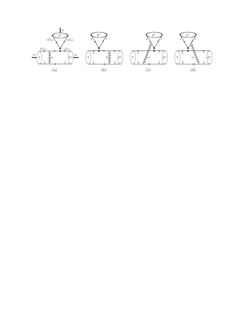
Figure 1: Feynman diagrams for the ${\Upsilon}$ ${\to}$ $B_{c}{\rho}$ decay with the pQCD approach, where (a) and (b) are factorizable emission diagrams, (c) and (d) are nonfactorizable emission diagrams.

II.5 Decay amplitudes

The Feynman diagrams for the ${\Upsilon}(1S)$ ${\to}$ $B_{c}{\rho}$ decay are shown in Fig.1, including factorizable emission topologies (a) and (b) where gluon connects to the quarks in the same meson, and nonfactorizable emission topologies (c) and (d) where gluon attaches to the quarks in two different mesons.

The amplitude for the ${\Upsilon}(1S)$ ${\to}$ $B_{c}{\rho}$ decay is defined as below prd66 ,

$${\cal A}({\Upsilon}(1S){\to}B_{c}{\rho})\ =\ {\cal A}_{L}({\epsilon}_{1}^{{\parallel}},{\epsilon}_{3}^{{\parallel}})+{\cal A}_{N}({\epsilon}_{1}^{{\perp}},{\epsilon}_{3}^{{\perp}})+i\,{\cal A}_{T}\,{\varepsilon}_{{\mu}{\nu}{\alpha}{\beta}}\,{\epsilon}_{1}^{{\mu}}\,{\epsilon}_{3}^{{\nu}}\,p_{1}^{\alpha}\,p_{3}^{\beta},$$ (33)

which is conventionally written as the helicity amplitudes prd66 ,

$${\cal A}_{0}\ =\ -C_{\cal A}\,\sum\limits_{i}{\cal A}_{L}^{i}({\epsilon}_{1}^{{\parallel}},{\epsilon}_{3}^{{\parallel}}),$$ (34)

$${\cal A}_{\parallel}\ =\ \sqrt{2}\,C_{\cal A}\sum\limits_{i}{\cal A}_{N}^{i}({\epsilon}_{1}^{{\perp}},{\epsilon}_{3}^{{\perp}}),$$ (35)

$${\cal A}_{\perp}\ =\ \sqrt{2}\,C_{\cal A}\,m_{1}\,p\sum\limits_{i}{\cal A}_{T}^{i},$$ (36)

$$C_{\cal A}\ =\ i\frac{G_{F}}{\sqrt{2}}\,\frac{C_{F}}{N}\,{\pi}\,f_{\Upsilon}\,f_{B_{c}}\,V_{cb}V_{ud}^{\ast},$$ (37)

where $C_{F}$ $=$ $4/3$ and the color number $N$ $=$ $3$; the superscript $i$ on ${\cal A}_{L,N,T}^{i}$ corresponds to the indices of Fig.1. The explicit expressions of building blocks ${\cal A}_{L,N,T}^{i}$ are collected in Appendix A.

III Numerical results and discussion

In the rest frame of the ${\Upsilon}(1S)$ meson, branching ratio (${\cal B}r$), polarization fractions ($f_{0,{\parallel},{\perp}}$) and relative phase between helicity amplitudes (${\phi}_{{\parallel},{\perp}}$) for the ${\Upsilon}(1S)$ ${\to}$ $B_{c}{\rho}$ weak decay are defined as

$${\cal B}r\ =\ \frac{1}{12{\pi}}\,\frac{p}{m_{{\Upsilon}}^{2}{\Gamma}_{{\Upsilon}}}\,\Big{\{}{|}{\cal A}_{0}{|}^{2}+{|}{\cal A}_{\parallel}{|}^{2}+{|}{\cal A}_{\perp}{|}^{2}\Big{\}},$$ (38)

$$f_{0,{\parallel},{\perp}}\ =\ \frac{{|}{\cal A}_{0,{\parallel},{\perp}}{|}^{2}}{{|}{\cal A}_{0}{|}^{2}+{|}{\cal A}_{\parallel}{|}^{2}+{|}{\cal A}_{\perp}{|}^{2}},$$ (39)

$${\phi}_{{\parallel},{\perp}}\ =\ {\arg}({\cal A}_{{\parallel},{\perp}}/{\cal A}_{0}),$$ (40)

where mass $m_{{\Upsilon}}$ $=$ $9460.30{\pm}0.26$ MeV and decay width ${\Gamma}_{\Upsilon}$ $=$ $54.02{\pm}1.25$ keV pdg .

The values of other input parameters are listed as follows. If not specified explicitly, we will take their central values as default inputs.

(1) Wolfenstein parameters pdg : $A$ $=$ $0.814^{+0.023}_{-0.024}$ and ${\lambda}$ $=$ $0.22537{\pm}0.00061$.

(2) Masses of quarks pdg : $m_{c}$ $=$ $1.67{\pm}0.07$ GeV and $m_{b}$ $=$ $4.78{\pm}0.06$ GeV.

(3) Gegenbauer moments $a^{\parallel}_{0}$ $=$ $1$ and $a^{\parallel}_{2}$ $=$ $0.15{\pm}0.07$ for twist-2 distribution amplitudes of the ${\rho}$ meson jhep0605 .

(4) Decay constants: $f_{{\Upsilon}}$ $=$ $(676.4{\pm}10.7)$ MeV fbb , $f_{B_{c}}$ $=$ $489{\pm}5$ MeV fbc , $f_{\rho}$ $=$ $216{\pm}3$ MeV jhep0605 .

Our numerical results are presented as follows:

$${\cal B}r\,=\,(8.34^{+0.47+1.35+0.40+1.44}_{-0.69-0.88-0.40-1.26}){\times}10^{-9},$$ (41)

$$f_{0}\,=\,(82.2^{+0.0+1.1+0.0}_{-0.7-1.3-0.0})\%,$$ (42)

$$f_{{\parallel}}\,=\,(15.0^{+0.6+1.0+0.0}_{-0.0-0.8-0.0})\%,$$ (43)

$$f_{\perp}\,=\,(2.8^{+0.1+0.3+0.0}_{-0.0-0.3-0.0})\%,$$ (44)

$${\phi}_{{\parallel}}\,{\simeq}\,0,\qquad{\phi}_{{\perp}}\,{\simeq}\,{\pi},$$ (45)

where the first uncertainty comes from the choice of the typical scale $(1{\pm}0.1)t_{i}$, and the expression $t_{i}$ is given in Eq.(71) and Eq.(72); the second uncertainty is from masses $m_{b}$ and $m_{c}$; the third uncertainty is from hadronic parameters including decay constants and Gegenbauer moments; and the fourth uncertainty of branching ratio comes from the CKM parameters. The following are some comments.

(1) Branching ratio for the ${\Upsilon}(1S)$ ${\to}$ $B_{c}{\rho}$ decay with the pQCD approach is different from previous estimation ijma14 ; adv2013 with the NF approximation. Many factors lead to these differences. For example, as it is showed in Ref. adv2013 , the values of form factors for ${\Upsilon}(1S)$ ${\to}$ $B_{c}$ transition are very sensitive to the choice of wave functions. In addition, form factors written as the convolution integral of wave functions in Ref. adv2013 are usually enhanced by one-gluon-exchange scattering amplitudes with the pQCD approach. These discrepancy deserve much dedicated study and should be carefully tested by the future experiments.

(2) Branching ratio for the ${\Upsilon}(1S)$ ${\to}$ $B_{c}{\rho}$ decay can reach up to ${\cal O}(10^{-9})$, which might be measurable at the running LHC and forthcoming SuperKEKB. For example, the ${\Upsilon}(1S)$ production cross section in p-Pb collision is about a few ${\mu}b$ at LHCb jhep1407 and ALICE plb740 . Over $10^{12}$ ${\Upsilon}(1S)$ data samples per $ab^{-1}$ data collected at LHCb and ALICE are in principle available, corresponding to a few thousands of the ${\Upsilon}(1S)$ ${\to}$ $B_{c}{\rho}$ events.

(3) There is a hierarchical pattern among the longitudinal $f_{0}$, parallel $f_{{\parallel}}$, and perpendicular $f_{{\perp}}$ polarization fractions, i.e.,

$$f_{0}:f_{{\parallel}}:f_{{\perp}}\ {\simeq}\ 1:\frac{p}{\sqrt{2}m_{{\Upsilon}(1S)}}:\frac{p^{2}}{2m_{{\Upsilon}(1S)}^{2}},$$ (46)

where $p$ is the common momentum of final state in the rest frame of the ${\Upsilon}(1S)$ meson. The relation Eq.(46) is basically agree with previous estimation adv2013 . It means that the contributions to branching ratio for the ${\Upsilon}(1S)$ ${\to}$ $B_{c}{\rho}$ decay mainly come from the longitudinal polarization fractions, because of $f_{0}$ $>$ $f_{{\parallel}}$ $>$ $f_{{\perp}}$.

(4) The relative phase ${\phi}_{{\parallel}}$ is close to zero. The reason is that the factorizable contributions from diagrams Fig.1(a,b) is real and proportional to the large coefficient $a_{1}$, while the nonfactorizable contributions from diagrams Fig.1(c,d) is suppressed by the color factor and proportional to the small Wilson coefficient $C_{2}$, and the strong phases arise only from the nonfactorizable contributions, which is consistent with the prediction of the QCD factorization approach qcdf1 ; qcdf2 where the strong phase arising from nonfactorizable contributions is suppressed by color and ${\alpha}_{s}$ for the $a_{1}$-dominated processes. The relative phases, if they could be determined experimentally, will improve our understanding on the strong interactions.

IV Summary

The ${\Upsilon}(1S)$ weak decay is allowable within the standard model. In this paper, the ${\Upsilon}(1S)$ ${\to}$ $B_{c}{\rho}$ weak decays are studied with the pQCD approach. It is found that with the nonrelativistic wave functions for ${\Upsilon}(1S)$ and $B_{c}$ mesons, the longitudinal polarization fraction is the largest one, and branching ratios for the ${\Upsilon}(1S)$ ${\to}$ $B_{c}{\rho}$ decay can reach up to ${\cal O}(10^{-9})$, which might be detectable at the future experiments.

Appendix A Building blocks of decay amplitudes

For the sake of simplicity, the amplitude for the ${\Upsilon}(1S)$ ${\to}$ $B_{c}{\rho}$ decay, Eq.(33), is decomposed into building blocks ${\cal A}^{i}_{L,N,T}$, where the superscript $i$ corresponds to the indices of Fig.1. With the pQCD master formula Eq.(5), the explicit expressions of ${\cal A}^{i}_{L,N,T}$ are written as follows:

$${\cal A}_{L}^{a} = {\int}_{0}^{1}dx_{1}{\int}_{0}^{1}dx_{2}{\int}_{0}^{\infty}b_{1}db_{1}{\int}_{0}^{\infty}b_{2}db_{2}\,{\phi}_{\Upsilon}^{v}(x_{1})$$ (47)

$${\phi}_{B_{c}}(x_{2})\,E_{f}(t_{a})\,{\alpha}_{s}(t_{a})\,a_{1}(t_{a})\,H_{f}({\alpha}_{e},{\beta}_{a},b_{1},b_{2})$$

$$\Big{\{}m_{1}^{2}\,s+m_{2}\,m_{b}\,u-(4\,m_{1}^{2}\,p^{2}+m_{2}^{2}\,u)\,\bar{x}_{2}\Big{\}},$$

$${\cal A}_{N}^{a} = m_{1}\,m_{3}{\int}_{0}^{1}dx_{1}{\int}_{0}^{1}dx_{2}{\int}_{0}^{\infty}b_{1}db_{1}{\int}_{0}^{\infty}b_{2}db_{2}\,{\phi}_{\Upsilon}^{V}(x_{1})$$ (48)

$${\phi}_{B_{c}}(x_{2})\,E_{f}(t_{a})\,{\alpha}_{s}(t_{a})\,a_{1}(t_{a})\,H_{f}({\alpha}_{e},{\beta}_{a},b_{1},b_{2})\,$$

$$\Big{\{}2\,m_{2}^{2}\,\bar{x}_{2}-2\,m_{2}\,m_{b}-t\Big{\}},$$

$${\cal A}_{T}^{a} = 2\,m_{1}\,m_{3}\,{\int}_{0}^{1}dx_{1}{\int}_{0}^{1}dx_{2}{\int}_{0}^{\infty}b_{1}db_{1}{\int}_{0}^{\infty}b_{2}db_{2}\,{\phi}_{\Upsilon}^{V}(x_{1})$$ (49)

$${\phi}_{B_{c}}(x_{2})\,E_{f}(t_{a})\,{\alpha}_{s}(t_{a})\,a_{1}(t_{a})\,H_{f}({\alpha}_{e},{\beta}_{a},b_{1},b_{2}),$$

$${\cal A}_{L}^{b} = {\int}_{0}^{1}dx_{1}{\int}_{0}^{1}dx_{2}{\int}_{0}^{\infty}b_{1}db_{1}{\int}_{0}^{\infty}b_{2}db_{2}$$ (50)

$${\phi}_{B_{c}}(x_{2})\,E_{f}(t_{b})\,{\alpha}_{s}(t_{b})\,a_{1}(t_{b})H_{f}({\alpha}_{e},{\beta}_{b},b_{2},b_{1})$$

$$\Big{\{}{\phi}_{\Upsilon}^{v}(x_{1})\,\Big{[}m_{1}^{2}\,(s-4\,p^{2})\,\bar{x}_{1}+2\,m_{2}\,m_{c}\,u-m_{2}^{2}\,u\Big{]}$$

$$+{\phi}_{\Upsilon}^{t}(x_{1})\,m_{1}\,\Big{[}s\,(2\,m_{2}-m_{c})-2\,m_{2}\,u\,\bar{x}_{1}\Big{]}\Big{\}},$$

$${\cal A}_{N}^{b} = m_{3}{\int}_{0}^{1}dx_{1}{\int}_{0}^{1}dx_{2}{\int}_{0}^{\infty}b_{1}db_{1}{\int}_{0}^{\infty}b_{2}db_{2}$$ (51)

$${\phi}_{B_{c}}(x_{2})\,E_{f}(t_{b})\,{\alpha}_{s}(t_{b})\,a_{1}(t_{b})\,H_{f}({\alpha}_{e},{\beta}_{b},b_{2},b_{1})$$

$$\Big{\{}{\phi}_{\Upsilon}^{V}(x_{1})\,m_{1}\,\Big{[}2\,m_{2}^{2}-4\,m_{2}\,m_{c}-t\,\bar{x}_{1}\Big{]}$$

$$+{\phi}_{\Upsilon}^{T}(x_{1})\,\Big{[}t\,(m_{c}-2\,m_{2})+4\,m_{1}^{2}\,m_{2}\,\bar{x}_{1}\Big{]}\Big{\}},$$

$${\cal A}_{T}^{b} = -2\,m_{3}\,{\int}_{0}^{1}dx_{1}{\int}_{0}^{1}dx_{2}{\int}_{0}^{\infty}b_{1}db_{1}{\int}_{0}^{\infty}b_{2}db_{2}$$ (52)

$${\phi}_{B_{c}}(x_{2})\,E_{f}(t_{b})\,{\alpha}_{s}(t_{b})\,a_{1}(t_{b})\,H_{f}({\alpha}_{e},{\beta}_{b},b_{2},b_{1})$$

$$\Big{\{}{\phi}_{\Upsilon}^{V}(x_{1})\,m_{1}\,\bar{x}_{1}+{\phi}_{\Upsilon}^{T}(x_{1})\,(m_{c}-2\,m_{2})\Big{\}},$$

$${\cal A}_{L}^{c} = \frac{1}{N_{c}}{\int}_{0}^{1}dx_{1}{\int}_{0}^{1}dx_{2}{\int}_{0}^{1}dx_{3}{\int}_{0}^{\infty}db_{1}{\int}_{0}^{\infty}b_{2}db_{2}{\int}_{0}^{\infty}b_{3}db_{3}$$ (53)

$${\phi}_{B_{c}}(x_{2})\,{\phi}_{\rho}^{v}(x_{3})\,E_{n}(t_{c})\,{\alpha}_{s}(t_{c})\,C_{2}(t_{c})\,H_{n}({\alpha}_{e},{\beta}_{c},b_{2},b_{3})$$

$${\delta}(b_{1}-b_{2})\,\Big{\{}{\phi}_{\Upsilon}^{v}(x_{1})\,u\,\Big{[}t\,x_{1}-2\,m_{2}^{2}\,x_{2}-s\,\bar{x}_{3}\Big{]}$$

$$+{\phi}_{\Upsilon}^{t}(x_{1})\,m_{1}\,m_{2}\,\Big{[}s\,x_{2}+2\,m_{3}^{2}\,\bar{x}_{3}-u\,x_{1}\Big{]}\Big{\}},$$

$${\cal A}_{N}^{c} = \frac{m_{3}}{N_{c}}{\int}_{0}^{1}dx_{1}{\int}_{0}^{1}dx_{2}{\int}_{0}^{1}dx_{3}{\int}_{0}^{\infty}db_{1}{\int}_{0}^{\infty}b_{2}db_{2}{\int}_{0}^{\infty}b_{3}db_{3}$$ (54)

$${\phi}_{B_{c}}(x_{2})\,E_{n}(t_{c})\,{\alpha}_{s}(t_{c})\,C_{2}(t_{c})\,H_{n}({\alpha}_{e},{\beta}_{c},b_{2},b_{3})$$

$$\Big{\{}{\phi}_{\Upsilon}^{V}(x_{1})\,{\phi}_{\rho}^{V}(x_{3})\,m_{1}\,\Big{[}2\,s\,\bar{x}_{3}+4\,m_{2}^{2}\,x_{2}\,-2\,t\,x_{1}\Big{]}$$

$$+{\phi}_{\Upsilon}^{T}(x_{1})\,{\phi}_{\rho}^{V}(x_{3})\,m_{2}\,\Big{[}2\,m_{1}^{2}\,x_{1}-t\,x_{2}-u\,\bar{x}_{3}\Big{]}$$

$$+{\phi}_{\Upsilon}^{T}(x_{1})\,{\phi}_{\rho}^{A}(x_{3})\,2\,m_{1}\,m_{2}\,p\,(x_{2}-\bar{x}_{3})\Big{\}}\,{\delta}(b_{1}-b_{2}),$$

$${\cal A}_{T}^{c} = \frac{m_{3}}{N_{c}\,p}{\int}_{0}^{1}dx_{1}{\int}_{0}^{1}dx_{2}{\int}_{0}^{1}dx_{3}{\int}_{0}^{\infty}db_{1}{\int}_{0}^{\infty}b_{2}db_{2}{\int}_{0}^{\infty}b_{3}db_{3}\,$$ (55)

$${\phi}_{B_{c}}(x_{2})\,E_{n}(t_{c})\,{\alpha}_{s}(t_{c})\,C_{2}(t_{c})\,H_{n}({\alpha}_{e},{\beta}_{c},b_{2},b_{3})$$

$$\Big{\{}{\phi}_{\Upsilon}^{V}(x_{1})\,{\phi}_{\rho}^{A}(x_{3})\,\Big{[}2\,s\,\bar{x}_{3}+4\,m_{2}^{2}\,x_{2}\,-2\,t\,x_{1}\Big{]}$$

$$+{\phi}_{\Upsilon}^{T}(x_{1})\,{\phi}_{\rho}^{A}(x_{3})\,r_{2}\,\Big{[}2\,m_{1}^{2}\,x_{1}-t\,x_{2}-u\,\bar{x}_{3}\Big{]}$$

$$+2\,m_{2}\,p\,{\phi}_{\Upsilon}^{T}(x_{1})\,{\phi}_{\rho}^{V}(x_{3})\,(x_{2}-\bar{x}_{3})\Big{\}}\,{\delta}(b_{1}-b_{2}),$$

$${\cal A}_{L}^{d} = \frac{1}{N_{c}}{\int}_{0}^{1}dx_{1}{\int}_{0}^{1}dx_{2}{\int}_{0}^{1}dx_{3}{\int}_{0}^{\infty}db_{1}{\int}_{0}^{\infty}b_{2}db_{2}{\int}_{0}^{\infty}b_{3}db_{3}$$ (56)

$${\phi}_{B_{c}}(x_{2})\,{\phi}_{\rho}^{v}(x_{3})\,E_{n}(t_{d})\,{\alpha}_{s}(t_{d})\,C_{2}(t_{d})\,H_{n}({\alpha}_{e},{\beta}_{d},b_{2},b_{3})$$

$${\delta}(b_{1}-b_{2})\,\Big{\{}{\phi}_{\Upsilon}^{t}(x_{1})\,m_{1}\,m_{2}\,\Big{[}s\,x_{2}+2\,m_{3}^{2}\,x_{3}-u\,x_{1}\Big{]}$$

$$+{\phi}_{\Upsilon}^{v}(x_{1})\,4\,m_{1}^{2}\,p^{2}\,(x_{3}-x_{2})\Big{\}},$$

$${\cal A}_{N}^{d} = \frac{m_{3}}{N_{c}}{\int}_{0}^{1}dx_{1}{\int}_{0}^{1}dx_{2}{\int}_{0}^{1}dx_{3}{\int}_{0}^{\infty}db_{1}{\int}_{0}^{\infty}b_{2}db_{2}{\int}_{0}^{\infty}b_{3}db_{3}$$ (57)

$${\phi}_{\Upsilon}^{T}(x_{1})\,{\phi}_{B_{c}}(x_{2})\,E_{n}(t_{d})\,{\alpha}_{s}(t_{d})\,C_{2}(t_{d})\,H_{n}({\alpha}_{e},{\beta}_{d},b_{2},b_{3})$$

$${\delta}(b_{1}-b_{2})\,\Big{\{}{\phi}_{\rho}^{V}(x_{3})\,m_{2}\,\Big{[}2\,m_{1}^{2}\,x_{1}-t\,x_{2}\,-u\,x_{3}\Big{]}$$

$$+2\,m_{1}\,m_{2}\,p\,{\phi}_{\rho}^{A}(x_{3})\,(x_{2}-x_{3})\Big{\}},$$

$${\cal A}_{T}^{d} = \frac{m_{3}}{N_{c}\,p}{\int}_{0}^{1}dx_{1}{\int}_{0}^{1}dx_{2}{\int}_{0}^{1}dx_{3}{\int}_{0}^{\infty}db_{1}{\int}_{0}^{\infty}b_{2}db_{2}{\int}_{0}^{\infty}b_{3}db_{3}$$ (58)

$${\phi}_{\Upsilon}^{T}(x_{1})\,{\phi}_{B_{c}}(x_{2})\,E_{n}(t_{d})\,{\alpha}_{s}(t_{d})\,C_{2}(t_{d})\,H_{n}({\alpha}_{e},{\beta}_{d},b_{2},b_{3})$$

$${\delta}(b_{1}-b_{2})\,\Big{\{}{\phi}_{\rho}^{A}(x_{3})\,r_{2}\,\Big{[}2\,m_{1}^{2}\,x_{1}-t\,x_{2}-u\,x_{3}\Big{]}$$

$$+2\,m_{2}\,p\,{\phi}_{\rho}^{V}(x_{3})\,(x_{2}-x_{3})\Big{\}},$$

where $\bar{x}_{i}$ $=$ $1$ $-$ $x_{i}$; variable $x_{i}$ and $b_{i}$ are the longitudinal momentum fraction and the conjugate variable of the transverse momentum $k_{i{\perp}}$ of the valence quark, respectively; ${\alpha}_{s}$ is the QCD coupling; $a_{1}$ $=$ $C_{1}$ $+$ $C_{2}/N$; $C_{1,2}$ are the Wilson coefficients.

The function $H_{f,n}$ and Sudakov factor $E_{f,n}$ are defined as follows, where the subscripts $f$ and $n$ correspond to factorizable and nonfactorizable topologies, respectively.

$$H_{f}({\alpha}_{e},{\beta},b_{i},b_{j})\ =\ K_{0}(\sqrt{-{\alpha}_{e}}b_{i})\Big{\{}{\theta}(b_{i}-b_{j})K_{0}(\sqrt{-{\beta}}b_{i})I_{0}(\sqrt{-{\beta}}b_{j})+(b_{i}{\leftrightarrow}b_{j})\Big{\}},$$ (59)

$$H_{n}({\alpha}_{e},{\beta},b_{2},b_{3}) = \Big{\{}{\theta}(-{\beta})K_{0}(\sqrt{-{\beta}}b_{3})+\frac{{\pi}}{2}{\theta}({\beta})\Big{[}iJ_{0}(\sqrt{{\beta}}b_{3})-Y_{0}(\sqrt{{\beta}}b_{3})\Big{]}\Big{\}}$$ (60)

$${\times} \Big{\{}{\theta}(b_{2}-b_{3})K_{0}(\sqrt{-{\alpha}_{e}}b_{2})I_{0}(\sqrt{-{\alpha}_{e}}b_{3})+(b_{2}{\leftrightarrow}b_{3})\Big{\}},$$

$$E_{f}(w)\ =\ {\exp}\{-S_{\Upsilon}(w)-S_{B_{c}}(w)\},$$ (61)

$$E_{n}(w)\ =\ {\exp}\{-S_{\Upsilon}(w)-S_{B_{c}}(w)-S_{\rho}(w)\},$$ (62)

$$S_{\Upsilon}(w)\ =\ s(x_{1},p_{1}^{+},1/b_{1})+2{\int}_{1/b_{1}}^{w}\frac{d{\mu}}{\mu}{\gamma}_{q},$$ (63)

$$S_{B_{c}}(w)\ =\ s(x_{2},p_{2}^{+},1/b_{2})+2{\int}_{1/b_{2}}^{w}\frac{d{\mu}}{\mu}{\gamma}_{q},$$ (64)

$$S_{\rho}(w)\ =\ s(x_{3},p_{3}^{+},1/b_{3})+s(\bar{x}_{3},p_{3}^{+},1/b_{3})+2{\int}_{1/b_{3}}^{w}\frac{d{\mu}}{\mu}{\gamma}_{q},$$ (65)

where $J_{0}$ and $Y_{0}$ ($I_{0}$ and $K_{0}$) are the (modified) Bessel function of the first and second kind, respectively; ${\gamma}_{q}$ $=$ $-{\alpha}_{s}/{\pi}$ is the quark anomalous dimension; the expression of $s(x,Q,1/b)$ can be found in the appendix of Ref.pqcd1 ; ${\alpha}_{e}$ is the gluon virtuality; the subscript of the quark virtuality ${\beta}_{i}$ corresponds to the indices of Fig.1. The definitions of the particle virtuality and typical scale $t_{i}$ are listed as follows:

$${\alpha}_{e} = \bar{x}_{1}^{2}m_{1}^{2}+\bar{x}_{2}^{2}m_{2}^{2}-\bar{x}_{1}\bar{x}_{2}t,$$ (66)

$${\beta}_{a} = m_{1}^{2}-m_{b}^{2}+\bar{x}_{2}^{2}m_{2}^{2}-\bar{x}_{2}t,$$ (67)

$${\beta}_{b} = m_{2}^{2}-m_{c}^{2}+\bar{x}_{1}^{2}m_{1}^{2}-\bar{x}_{1}t,$$ (68)

$${\beta}_{c} = x_{1}^{2}m_{1}^{2}+x_{2}^{2}m_{2}^{2}+\bar{x}_{3}^{2}m_{3}^{2}$$ (69)

$$- x_{1}x_{2}t-x_{1}\bar{x}_{3}u+x_{2}\bar{x}_{3}s,$$

$${\beta}_{d} = x_{1}^{2}m_{1}^{2}+x_{2}^{2}m_{2}^{2}+x_{3}^{2}m_{3}^{2}$$ (70)

$$- x_{1}x_{2}t-x_{1}x_{3}u+x_{2}x_{3}s,$$

$$t_{a(b)} = {\max}(\sqrt{-{\alpha}_{e}},\sqrt{-{\beta}_{a(b)}},1/b_{1},1/b_{2}),$$ (71)

$$t_{c(d)} = {\max}(\sqrt{-{\alpha}_{e}},\sqrt{{|}{\beta}_{c(d)}{|}},1/b_{2},1/b_{3}).$$ (72)