FERMILAB-TM-2617-AD-CD-E

Calibration and GEANT4 simulations of the Phase II Proton Compute Tomography (pCT) Range Stack Detector

1 Introduction

Northern Illinois University in collaboration with Fermi National Accelerator Laboratory (FNAL) and Delhi University has been designing and building a proton CT scanner [1] for applications in proton treatment planning. In proton therapy, the current treatment planning systems are based on X-ray CT images that have intrinsic limitations in terms of dose accuracy to tumor volumes and nearby critical structures. Proton CT aims to overcome these limitations by determining more accurate relative proton stopping powers directly as a result of imaging with protons. Fig. 1 shows a schematic proton CT scanner, which consists of eight planes of tracking detectors with two X and two Y coordinate measurements both before and after the patient. In addition, a calorimeter consisting of a stack of thin scintillator tiles, arranged in twelve eight-tile frames, is used to determine the water equivalent path length (WEPL) of each track through the patient. The X-Y coordinates and WEPL are required input for image reconstruction software to find the relative (proton) stopping powers (RSP) value of each voxel in the patient and generate a corresponding 3D image. In this note we describe tests conducted in 2015 at the proton beam at the Central DuPage Hospital in Warrenville, IL, focusing on the range stack calibration procedure and comparisons with the GEANT 4 range stack simulation.

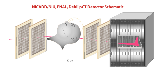
Figure 1: Four (X,Y) stations measure the proton trajectory before and after the patient. A stack of 3.2 mm thick scintillator tiles measures the residual energy or range after the patient.

2 The GEANT 4 model

To verify measurements obtained by the scanner at the CDH proton beam the scanner response was simulated using a detailed model based on the GEANT-4 software. Fig. 2 shows a spherical water phantom between the tracker planes of the scanner model. The simulated responses of the range stack and tracker stations were analyzed with the same software as for the data.

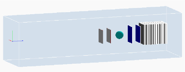
Figure 2: The GEANT4 visualization of the scanner model used in the simulations.

3 The CDH test beam

Figure 3 shows the NIU scanner mounted on a cart in a treatment room at Central DuPage Hospital. The proton beam enters the upstream tracker planes from the right followed by the downstream tracker planes and finally the range stack. In this note the range stack tiles are labeled from zero (the tile closest to the tracker) to 95. Data were obtained using proton beams of energy in range from 103-225 MeV, equivalent to 8-32 cm proton stopping range in water.

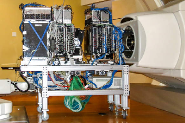
Figure 3: Fully assembled proton CT scanner at CDH Proton center. From right to left, beam enters the upstream tracker planes followed by the downstream tracker planes and finally the range stack. The gap in the middle is the position of the rotation stage for the head phantom in the horizontal plane.

3.1 Data acquisition (DAQ) system and event selection

The DAQ system of the scanner is described in  [2]. The range stack data are collected by twelve front-end boards. Each board provides the readout of one eight-tile range stack frame in form of time-stamped records of signal amplitudes in all tiles of the frame. We form the proton candidate event by combining records with close time-stamps. We remove events candidates with duplicated frames (overlapped tracks). We then found the frame with a Bragg peak, or stopping frame, and check that all frames before the stopping frame are also present in the event.

3.2 Units of measurement

The CDH accelerator control system is tuned to operate with proton beams with energies expressed in units of the proton stopping range in water in $cm$, $R_{w}(cm)$. One can also express the proton stopping range $R_{w}$, and thus the beam energy $E_{beam}$, in density-independent units of $g/cm^{2}$ :

$$E_{beam}(g/cm^{2})\equiv R_{w}(g/cm^{2})=R_{w}(cm)\times\rho_{w}(g/cm^{3})$$ (1)

To obtain the energy $E_{beam}$ in $MeV$ we use proton energy-range tables (a.k.a. Janni’s tables) [4]. A fit of the stopping range $R_{w}(g/cm^{2})$ as a function of $E(MeV)$ is shown in Fig. 4(a). We use

$$R_{w}(g/cm^{2})=0.0022\times E_{MeV}^{(1.77)}$$ (2)

to convert beam energies between $MeV$ and $g/cm^{2}$ units.

We calculate the proton stopping range in the range stack $R_{rs}(g/cm^{2})$ using the measured proton stopping position as described in Section 5. We compare the $R_{rs}(g/cm^{2})$ with the range calculated from the total energy measured by the range stack using the energy-range dependence in polystyrene shown in Fig. 4(b).

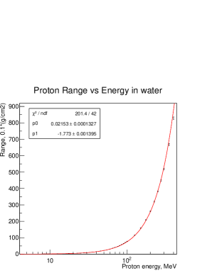
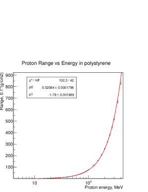
                          (a)                        (b)

Figure 4: a) The proton stopping range in water $R_{w}(g/cm^{2})$ (black dots) versus proton energy $E(MeV)$, as measured in [4]. The fit $R_{w}(g/cm^{2})=0.0022\times E_{MeV}^{(1.77)}$ conversion function (the red line) is used to find beam energies in $MeV$ that correspond to nominal CDH energies in $cm$. b) The proton stopping range in polystyrene $R_{poly}(g/cm^{2})$ (black dots) versus proton energy $E(MeV)$.

4 Stack calibration procedure

Energy deposition in each range stack scintillator tile is measured by two SiPMs connected to the tile’s single wavelength shifting (WLS) fiber. After passage of a proton, for each of the two SiPMs the maximum digitized signal, $A^{max}_{SiPM}$, is collected by the DAQ system. Thus the measured energy deposition in each range stack tile, $A^{ADC}_{tile}$, is obtained as a sum of $A^{max}_{SiPM}$ signals from SiPMs connected to this tile. This measurement varies from tile to tile even for protons of similar energy due to differences in the SiPM’s properties and the settings of corresponding readout channels. The following four step procedure is applied to calibrate the range stack detector.

1) We measure pedestal amplitudes $A^{pdSiPM1}_{tn}$, $A^{pdSiPM2}_{tn}$ and amplitudes $A^{1peSiPM1}_{tn}$,
$A^{1peSiPM2}_{tn}$ of the first photo-electron (PE) peak for all range stack tiles, $tn$, by collecting events with no beam. Fig. 5(a) and Fig. 5(b) show these distributions for SiPM1 and SiPM2 of Tile0. The combined SiPM1+SiPM2 no-beam signal in Tile0 is shown in Fig. 5(c). Figure 6 shows calibration signals for all 16 SiPMs of the first range stack frame. From these data the ADC to PE conversion coefficients for each SiPM are calculated as

$$K^{peSiPM}_{tn}=A^{1peSiPM}_{tn}-A^{pdSiPM}_{tn}$$

Ratios of PE conversion coefficients $K^{peSiPM0}_{tn}/K^{peSiPM0}_{t0}$ of the first and second SiPM in each tile to the conversion coefficient in the first SiPM in Tile0 are shown in Fig. 7(a) and Fig. 7(b). Most sensors have a response within 10% of one another.

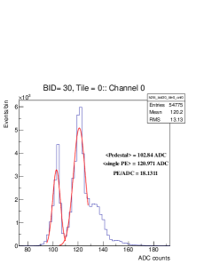
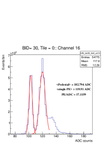
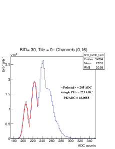
                          (a)                        (b)                        (c)

Figure 5: Measured Tile0 signal amplitudes : a) pedestal and the first photo-electron (PE) peak in the SiPM1 of Tile 0 in events with no beam. b) pedestal and the first photo-electron (PE) peak in the SiPM2 of Tile 0 in events with no beam. c) SiPM1+SiPM2 combined.

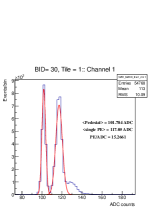
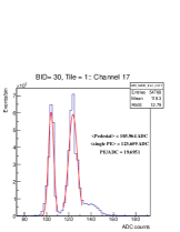
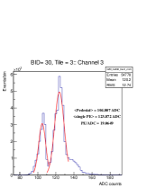
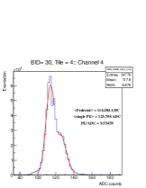
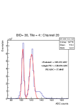
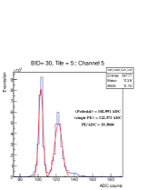
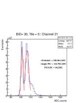
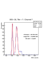
Figure 6: No beam signals used for PE calibration for the first eight tiles of the range stack.

2) The proton energy deposition in each tile $E^{pe}_{tn}$ in PE units is obtained via

$$E^{pe}_{tn}=(A^{sSiPM1}_{tn}-A^{pdSiPM1}_{tn})/K^{peSiPM1}_{tn}+(A^{sSiPM2}_{tn}-A^{pdSiPM2}_{tn})/K^{peSiPM2}_{tn}$$.

Fig. 8(a) and Fig. 8(b) show the PE signals of SiPM1 and SiPM2 in Tile0, Fig. 8(c) shows the combined SiPM1+SiPM2 signal, $A^{pe}_{t0}$, in Tile0.

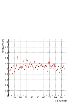
                          (a)                        (b) hfill

Figure 7: a) The ratio of PE conversion coefficients $K^{peSiPM0_{tn}}/K^{peSiPM0_{t0}}$ for the first SiPMs. b) The ratio of PE conversion coefficients $K^{peSiPM1_{tn}}/K^{peSiPM0_{t0}}$ for the second SiPMs.

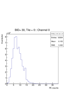
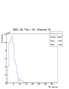
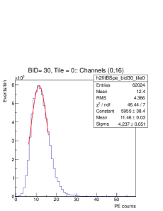
                          (a)                        (b)                        (c)

Figure 8: Measured signal amplitudes (PE units) in Tile0 at a beam energy of 26 cm (200 MeV) after subtracting pedestals : a) in SiPM1; b) in SiPM2; c) sum of SiPM1 and SiPM2. The means of Gaussian fits of combined signals away from the Bragg peak at a beam energy of 32 cm (225 MeV) were used to extract the normalization coefficients for the range stack tiles.

3) We measure signals $E^{clbExp}_{tn}$ of all range stack tiles in the region far away from the Bragg peak. We conducted two calibration runs at an energy of 32 cm (225 MeV). For the second run, the assembled scanner was turned 180 degrees to expose the back tiles to the beam first. The “front” run is used to calibrate the first front 48 tiles of the stack, while the “back” run is used to calibrate the 48 back tiles. We assume that the “true” $E^{clbTrue}_{tn}$ amplitudes of the tile signals follow energy profiles calculated from proton energy-range tables for polystyrene (the material used for the range stack tiles).

Figure 9(a) shows the tabulated proton dE/dx dependence. Fig. 9(b) and Fig. 9(c) show energy profiles calculated for protons entering the range stack with energies of 30.6 cm in the “front” run and 31.4 cm in the “back” run (corrections to the nominal CDH accelerator energy were applied to account for material in the tracker which is only present in the “front” run configuration and material in the CDH beam transport line, as discussed in Section 5.3). All “true” $E^{clbTrue}_{tn},tn=0,95$ amplitudes are normalized to the signal $E^{clbExp}_{t0}$ of the Tile0 in the “front” run. That is, we take the observed energy in Tile0 as to be correct.

The comparison of signals observed in Tile0 in runs of different energies and expected signals obtained by integration of the tabulated proton dE/dx dependence are shown in Fig. 10. The expected signals are normalized to the mean Tile0 data signal in the 32 cm run. The measured and calculated amplitudes are in good agreement, however the data signals are about 5% higher at low proton energies.
4) We extract normalization coefficients $K^{clb}_{tn}\equiv{E^{clbTrue}_{tn}\over E^{clbExp}_{tn}}$ and use them in all data runs to correct the observed signals in the range stack tiles. Figures 11(a) and (b) show the corrected energy deposition profiles (the mean number of photoelectrons from about 10000 protons per tile as function of tile number) for 200 MeV protons. Corrected energy profiles for different beam energies are shown in Fig. 12 through Fig. 14. Slight variations are attributed to statistical effects.

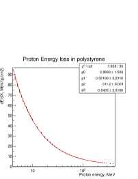
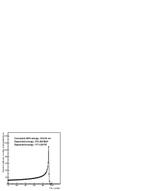
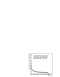
                          (a)                        (b)                        (c)

Figure 9: a) The proton dE/dX dependency in polystyrene as tabulated in Janni’s proton energy-range tables. b) The “true” front run signal profile used for calibration of tiles (0-47) of the range stack. c) The “true” back run signal profile used for calibration of tiles (48-95) of the range stack.

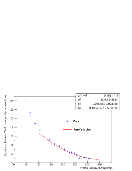
Figure 10: Measured signal amplitudes (blue crosses) and expected amplitudes calculated from Janni’s tables (red line) in Tile0 of the range stack for different proton energies. The expected signals normalized to the mean (over 10000 protons) Tile0 data signal in the 32 cm run.

                                       (a)                                (b)

Figure 11: The mean number of photoelectrons in the range stack tiles as a function of tile number produced by protons with energy 26 cm (200 MeV) (a) raw; (b) calibrated. The errors bars reperesent $\pm 1$ sigmas of Gaussian fits about the average, for an example see Fig. 8(c) .

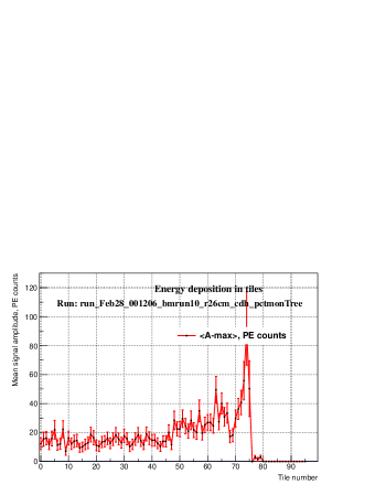
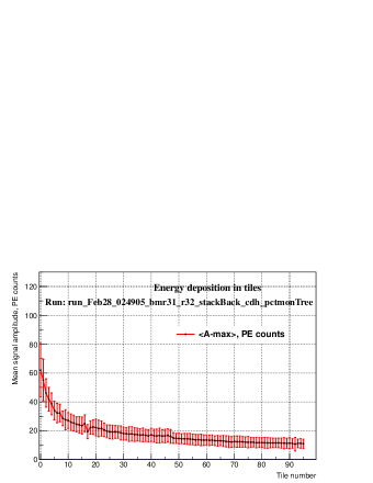
                                       (a)                                (b)

Figure 12: The mean number of photoelectrons in the range stack tiles as a function of tile number produced by protons with energy (a) 32 cm (225 MeV), “front” run ; (b) 32 cm (225 MeV), “back” run, no tracker. The errors bars reperesent $\pm 1$ sigmas of Gaussian fits about the average.

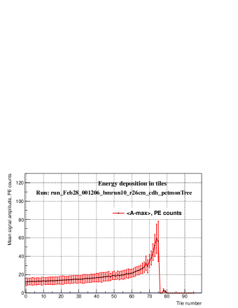
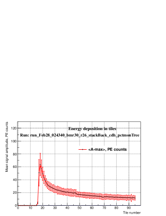
                                       (a)                                (b)

Figure 13: The mean number of photoelectrons in the range stack tiles as a function of tile number produced by protons with energy (a) 26 cm (200 MeV, “front run” ) ; (b) 26 cm (200 MeV, “back run” ), no tracker. The errors bars reperesent $\pm 1$ sigmas of Gaussian fits about the average. The three tile difference in the stopping position ($nt_{stop}$ = 74 in the front run, while $nt_{stop}$=77 in the back run run without the tracker) agrees with the tracker stopping power,  $3.2\times 1.01\times 3=0.97$ cm.

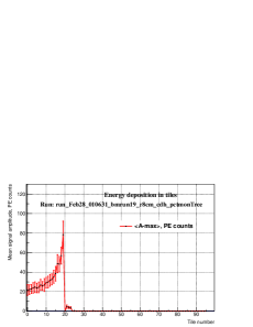
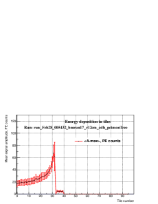
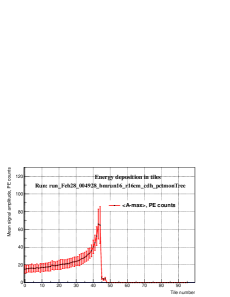
                         (a)                                     (b)                                     (c)

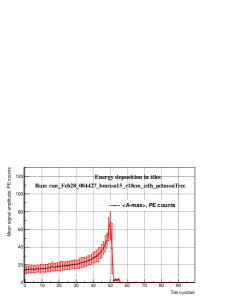
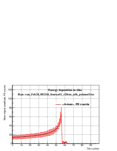
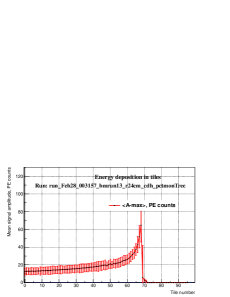
                         (d)                                     (e)                                     (f)

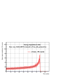
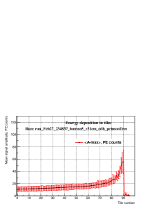
                         (g)                                     (h)                                     (i)

Figure 14: The mean number of photoelectrons in the range stack tiles as a function of tile number produced by protons with energy (a) 8 cm (103 MeV); (b) 12 cm (117 MeV); (c) 16 cm (129 MeV); (d) 18 cm (162 MeV) ; (e) 20 cm (172 MeV); (f) 24 cm (191 MeV); (g) 25 cm (196 MeV) ; (h) 27 cm (204 MeV); (i) 31 cm (221 MeV).

5 Range and energy measurements

The NIU image reconstruction software uses the WEPL of a scanned object, $wepl_{obj}$. For each proton the $wepl_{obj}$ can be obtained from WEPL of the range stack, $wepl_{rs}$,

$wepl_{obj}=E_{beam}(cm)-wepl_{rs}$,

To find $wepl_{rs}$ one need calibrate the total energy $E_{rs}$ or the stopping range $R_{rs}$ measured by the range stack detector using a set of phantoms with known WEPL [3]. Here we compare the accuracy of $R_{rs}$ and $E_{rs}$ to choose what measurement is preferrable for the WEPL calibration.

To find the total energy $E_{rs}$ deposited in the range stack we first search for the frame with a stopping tile (the “stopping” frame), then sum signals (in PE units) from all tiles and all frames including the stopping frame. Only events with no missing frames before the stopping frame were selected. Figure 15(a) shows the total $E_{rs}$ in PE measured in a run with $E_{beam}=26$ cm.

To find $R_{rs}$ we use the $Z$-position of the tile with the maximum signal (the “stopping” tile, labeled as $nt_{stop}$). We calculate $R_{rs}$ as

$$\begin{split}R_{rs}=(nt_{stop}+1)\times(tileW\times tileD+alW\times alD+mlrW\times mlrD)+\\ nframe\times(alW\times alD+mlrW\times mlrD),nt_{stop}=[0,95];nframe=[0,11]\end{split}$$

where $(tileW,alW,mlrW)=(3.2,0.00022,0.00625)~{}mm$ are the widths of scintillator and wrapper (aluminized mylar) layers, and $(tileD,alD,mlrD)=(1.011,2.700,1.397)~{}g/cm^{3}$ are the densities of these materials. The second term accounts for the extra layer of the wrapper in the end of each range stack frame.

Note, the stopping ranges in polysterene and mylar expressed in $g/cm^{2}$ are approximately equal to the proton stopping range in water $R_{w}$:

$$R_{w}(cm)=\int^{R_{m}}_{0}RSP_{m}dL$$ (3)

where $RSP_{m}$ is the proton stopping power of the medium relative to water and $L$ is the physical proton path length along the calorimeter and $R_{m}$ is the physical depth at which the proton stops in the range stack. Then, neglecting small variations ( $<0.5\%$) in mean ionization potential between water, polystyrene and mylar, as used in the Bethe Bloch equation, the water equivalent range of the proton becomes

$$R_{w}(cm)\simeq\int^{R_{m}}_{0}\rho_{m}/\rho_{w}dL,and,for\rho_{w}=1.0~{}g/cm^{3},R_{w}(g/cm^{2})\simeq\int^{R_{m}}_{0}\rho_{m}dL$$

Thus we expect $R_{rs}$ to have linear dependency on the beam energy, $E_{beam}$, expressed in $cm$. Figure 16 shows $R_{rs}$ in a run with $E_{beam}=26$ cm.

We also can find the $R_{rs}$ from the total energy $E_{rs}$ using Janni’s range-energy tables This method requires expression of $E_{rs}$ in MeV, and we use the conversion coefficient calculated as the ratio of the mean amplitude of the data signal (in number of photoelectrons) to the mean amplitude of the estimated MC signal (in MeV) in Tile0, in 26 cm runs. Figure 15(b) shows the proton stopping range in the range stack $R_{rs}^{conv}(g/cm^{2})$ calculated from $E_{rs}$ via the $R^{conv}_{rs}=0.0021\times E_{rs}^{(1.78)}$ conversion function obtained from Janni’s tables. Finally, we can find $wepl_{rs}$ directly, from the WEPL of a scanned object calculated from $E_{rs}$ using the Bethe-Bloch equation. Howewer, this will also require calibration, as the measured $E_{rs}$ only includes the visible part of deposited energy. Figure 15(c) shows the WEPL of the range stack $wepl^{calc}_{rs}(cm)$ calculated from $E_{rs}$ via

$$wepl^{calc}_{rs}=E_{beam}(cm)-\int^{E_{rs}}_{E_{beam}}\frac{1}{S(E_{p})}dE$$ (4)

where $S(E_{p})=-dE/dx$ is a water stopping power for proton with energy $E_{p}$.

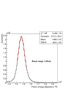
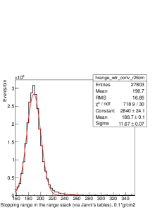
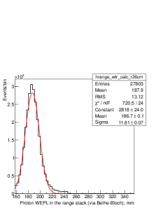
                    (a)                              (b)                              (c)

Figure 15: (a) the total energy, $E_{rs}$, in $PE$ measured with the range stack detector in a $E_{beam}=26~{}cm$ run; (b) the proton stopping range in the range stack $R_{rs}^{conv}(g/cm^{2})$ obtained from $E_{rs}$ via $R_{rs}^{conv}=0.0022\times E_{rs}^{(1.77)}$; (c) the proton WEPL in the range stack $wepl^{calc}_{rs}$, $mm$ calculated from $E_{rs}$ via energy loss equation.

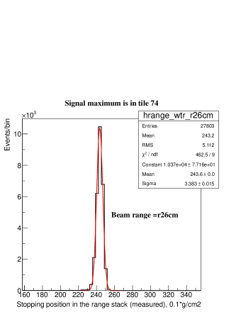
Figure 16: The measured proton stopping range, $R_{rs}$, in the range stack, $E_{beam}=26~{}cm$ run.

We fit peaks of the $R_{rs}$ and $E_{rs}$ distributions with a Gaussian and use the mean and $\sigma$ parameters of the fits to study the linearity ($R_{rs}$ and $E_{rs}$ as functions of the beam energy) and resolution ($\sigma(E_{rs})/E_{rs}$ and $\sigma(R_{rs})/R_{rs}$ as functions of $E_{rs}$ and $R_{rs}$) of the range stack detector. The linearity and resolution plots for the proton stopping position $R_{rs}$ are shown in Fig. 17 and the linearity and resolution plots for the energy measurement are shown in Fig. 18. The good linearity with a non zero intercept of the $R_{rs}$ shows there is material in front of the range stack at all energies. The energy measurement has lower accuracy (energy resolution ranges from 5.5% to 3.5% , compared to 2.2-1.2% for $R_{rs}$) and also shows an unexpected suppression at beam energies of 27 cm and 28 cm. Additionally, Figures 15(a) and (b) show that if we try to extract the stopping range or WEPL in the range stack from the direct energy measurement, the $R^{conv}_{rs}$ and distributions with $\sigma(R^{conv}_{rs})=11.7~{}mm$ and $\sigma(wepl^{calc}_{rs})=11.8~{}mm$ are significantly wider than $R_{rs}$ distribution with $\sigma({R}_{rs})=3.3~{}mm$. Thus, the direct $R_{rs}$ measurement is preferred for the WEPL calibration.

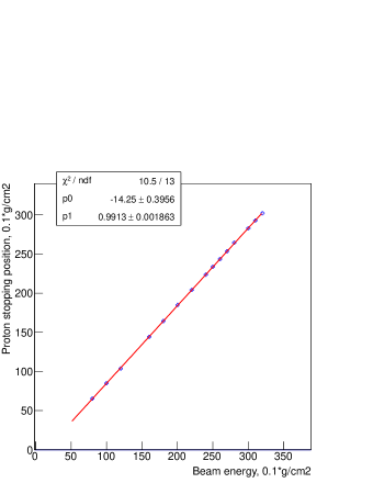
                                       (a)                                (b)

Figure 17: (a) The linearity of the directly measured proton stopping position measurement $R_{rs}$ ; (b) the $R_{rs}$ resolution. The linearity fit allows an estimate of the width of the extra material in front of the range stack ($\approx$14.0 mm).

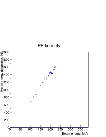
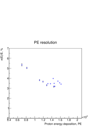
                                       (a)                                (b)

Figure 18: (a) the linearity of the energy measurement $E_{rs}$; (b) the $E_{rs}$ resolution.

5.1 Comparison with GEANT 4 simulations

A GEANT 4 simulation of the pCT detector was used to obtain the energy deposition $E^{g4}_{tn}$ in the range stack tiles for different beam energies. We converted the range $R_{p}$ to energy $E_{p}$ using the inverse of the Janni fit:

$E_{p}=(R_{p}/0.0022)^{(1/1.77)}$.

To compare energy profiles and total energy deposition in the range stack, the G4 signals in the tiles were expressed in the number of photoelectrons by normalizing to the data signal in Tile0 in the 26 cm beam run.

5.2 Smearing of simulated tile signals

To account for photo-statistics and SiPM readout, smearing of the G4 signals in each tile was done as:

$S^{g4}_{tn}=G(<S^{ped}_{tn}>)+P(E^{g4}_{tn})-<S^{ped}_{tn}>$

,
where $<S^{ped}_{tn}>$ is a mean sum of SiPM pedestals in tile $n$ from calibration runs, $E^{g4}_{tn}$ is the energy deposition in tile $n$ obtained from GEANT, and $G(S^{ped}_{tn})$ and $P(E^{g4}_{tn})$ are the sum of SiPM pedestals smearing using Gaussian and $E^{g4}_{tn}$ smeared using Poisson distribution. The effect of smearing is shown in Fig. 19, where the left plot shows the total energy deposition in the range stack at a beam energy of 26 cm (or 200 MeV) in data; the center histogram shows the unsmeared simulated signal, and the right histogram shows the smeared signal. Comparison of data and simulated signals from 200 MeV protons in Tile0 and in Tile74 (the stopping tiles with the maximal signal for this energy) are shown in Fig. 20.

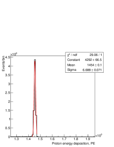
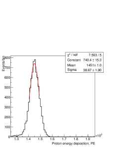
                    (a)                              (b)                              (c)

Figure 19: (a) the total energy deposition in the range stack at beam energy of 26 cm (200 MeV ) in data; (b) the unsmeared total energy deposition in the range stack at beam energy of 26 cm (200 MeV) in GEANT; (c) the smeared range stack energy measurement at beam energy of 26 cm (200 MeV) in GEANT.

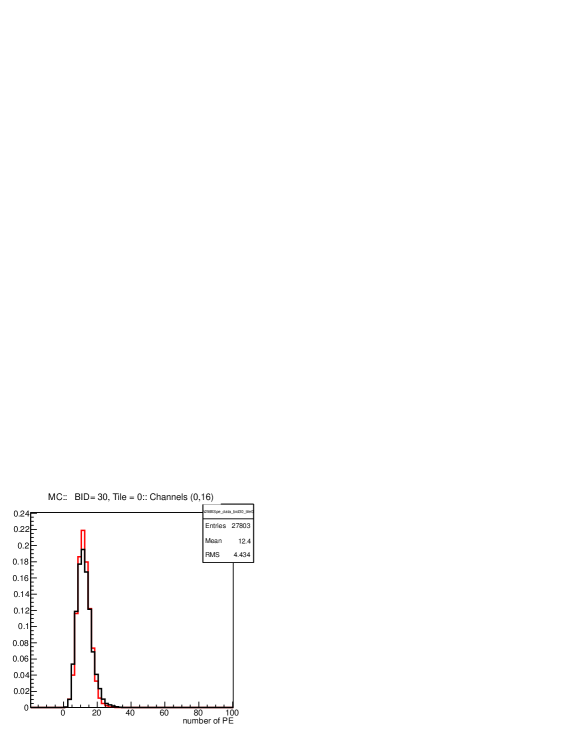
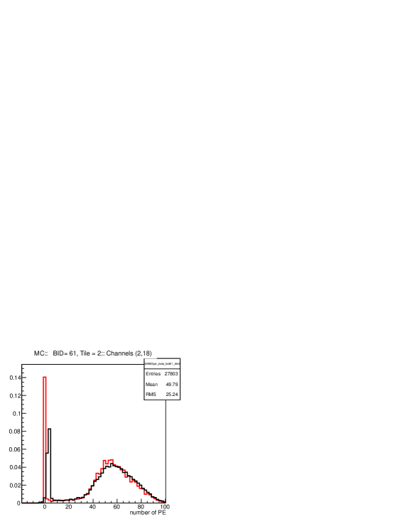
                                       (a)                                (b)

Figure 20: Comparison of data (blue histograms) and simulated signals (red histograms) from 200 MeV protons in (a) Tile0 and (b) Tile74 (the stopping tile, maximal signal).

5.3 Beam energy correction and smearing for the MC simulations

The total stopping range of all material along the proton path, $R_{total}$, before the proton stopping position is equal to the nominal beam energy of the accelerator in $g/cm^{2}$, $R_{total}\equiv E^{beam}_{total}$. In our test beam configuration, the total stopping range can be expressed as:

$$R_{total}=R_{rs}+R_{beamline}+R_{tracker}+sft\_const,\\$$

where $R_{rs}$, $R_{beamline}$, $R_{tracker}$ are the proton ranges in the range stack, any material in the accelerator beam line, and the tracker, respectively.

The $sft\_const$ is the systematic shift of the range measurement due to initial and arbitrary origin of the range calculation. We extract the stopping range using the position of the tile with the maximum signal and the total width of scintillator and wrapping layers including this stopping tile. The definition of stopping position is arbitrary and for consistency estimated with the MC. We estimate the $sft\_const$ using simulations of the range stack response in configuration with no tracker. In the GEANT model we do not have any other material before the range stack, and the $sft\_const$ can be obtained from the fit of the proton stopping positions at different beam energies, as shown in Fig. 21(a). Evaluation of the fit function at zero beam energy results in $sft\_const$=$0.7\pm 0.4$ mm in water (the $-p0$ parameter of the fit). From the fit of the measured proton stopping position $R_{rs}$ in Fig. 17(a) the $R_{beamline}+R_{tracker}+sft\_const$ is equal to $14.3\pm 0.4$ mm. This means that the proton energy at the range stack entry point, $Ep_{entry}$, is lower than the nominal accelerator beam energy by $13.6\pm 0.5$ mm (after subtracting the 0.7 mm $sft\_const$ parameter) for all test runs. To accurately compare the energy and range measurement with simulations, the $Ep_{entry}$ should be the same in data and in MC. Figure 21(b) shows the simulated proton stopping positiom $R_{rs}$ in a configuration with the tracker, and here the $R_{tracker}+sft\_const$ is equal to $7.9\pm 0.5$ mm (again 0.7 mm is subtracted from the $-p0$ parameter of the fit). Thus for simulations we subtract the difference of 5.7 mm (between the 13.6 mm observed in data and the 7.9 mm observed in MC) from all nominal beam energy points in GEANT runs to compensate. The corrected results are shown in Fig. 21(c) and now the $Ep_{entry}$ in GEANT runs is equal to the $Ep_{entry}$ in data runs.

Simulations also predict that this method of upstream material width estimation from the range stack measurements works with an accuracy of about 0.5 mm in a configuration with a variable width of a rectangular water phantom installed before the range stack. For the water phantom width of 2 mm, 5 mm, 10 mm, and 15 mm the simulated measurements are 2.1 mm, 5.4 mm, 10.3 mm and 14.3 mm, respectively.

Additionally we smear $Ep_{entry}$ in GEANT in a range between 0.05% at 100 MeV to 0.02% at 200 MeV to account for the CDH beam energy spread.

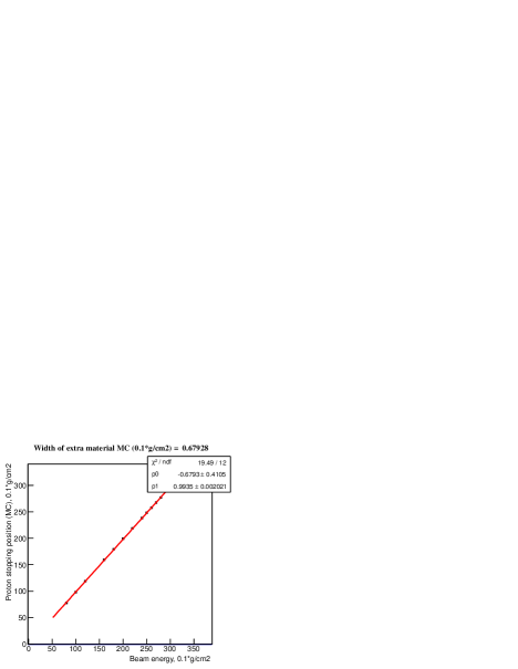
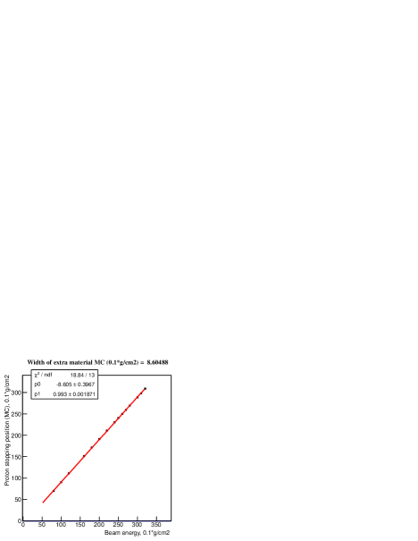
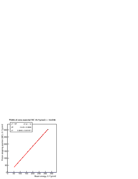
                    (a)                              (b)                              (c)

Figure 21: (a) the linearity of the proton stopping position measurement $R_{rs}$ obtained with GEANT using the nominal CDH beam energy points in a configuration with no tracker before the range stack; (b) the $R_{rs}$ linearity for nominal CDH beam energy points including the tracker; (c) the $R_{rs}$ linearity after correcting beam energies by adding “extra material” observed in data (5.7 mm).

5.4 Comparison of proton stopping position measurements

The linearity and resolution plots for the proton stopping position $R_{rs}$ are shown in Fig. 22. Fits correspond to the simulated results. We observe excellent agreement both in linearity and resolution. We used the detector model in which the density of the scintillator tiles is decreased by 1% compare to the nominal value of $1.025\pm 0.010$ $g/cm^{3}$, which provides the best agreement between measured and simulated proton stopping positions for different beam energies, as shown in Figure 23.

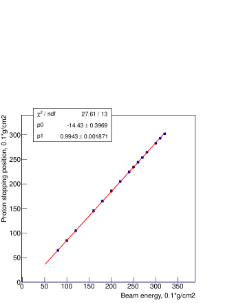
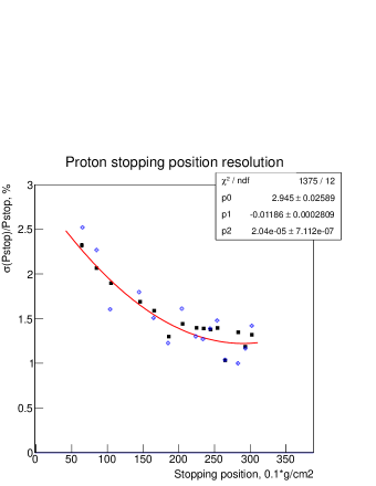
                                       (a)                                (b)

Figure 22: Comparison of (a) the linearity and (b) resolution of the proton stopping position measurement $R_{rs}$ in data and GEANT. Fits correspond to simulated results (black squares). Data shown as “blue crosses“.

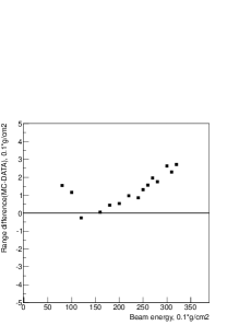
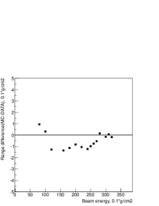
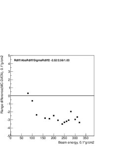
                    (a)                              (b)                              (c)

Figure 23: The difference between measured and simulated proton stopping positions for a GEANT models with (a) nominal scintillator density of $1.025\pm 0.010$ $g/cm^{3}$; (b) nominal density decreased by 1% (used in this Note); (c) nominal density decreased by 2%.

5.5 Comparison of energy measurements

The linearity and resolution plots for the energy measurements $E_{rs}=\sum E_{tn}$ in the range stack are shown in Fig. 24. Fits correspond to the simulated results. The instrumental depression in the data linearity plot at beam energies of 27 cm and 28 cm is not present in simulations. The MC model response shows good linearity. The resolution is between 4% and 2% that is higher than observed in data (between 5% and 3%). A comparison of measured (blue crosses) and simulated (black square) energy measurements in Tile0 for different proton energies is shown in Fig. 25.

The normalized simulated energy amplitude profiles in the range stack in Fig. 27 (red histograms) show fair agreement with the calibrated data (black dots) but diverge in amplitude at low proton energies (consistent with Fig. 25). The divergence could be due to higher event rates in high proton energy runs, shown in Fig. 26.

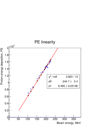
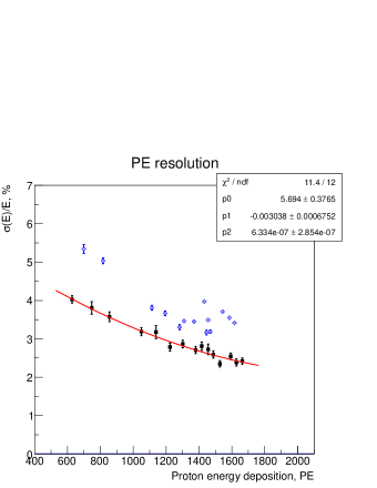
                                       (a)                                (b)

Figure 24: Comparison of (a) the linearity and (b) resolution of the energy measurements in the range stack in data and GEANT. Fits correspond to simulated results (black squares). Data shown as “blue crosses“.

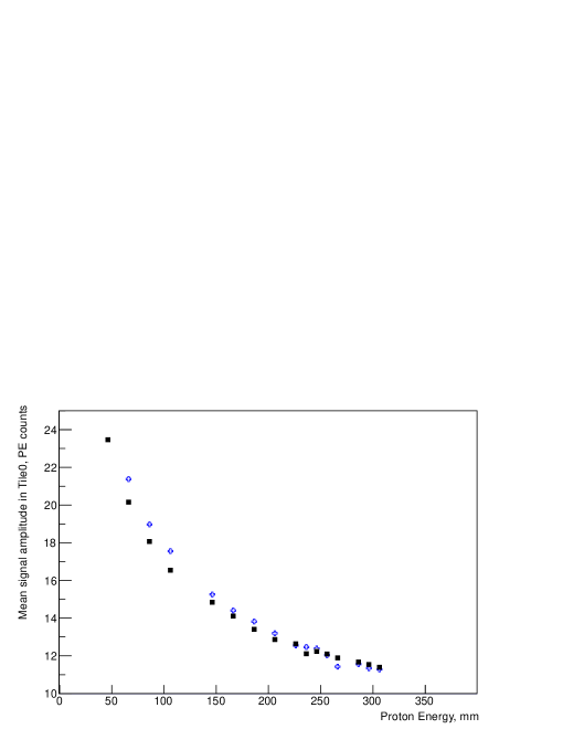
Figure 25: Comparison of the measured (blue crosses) and simulated (black square) signal amplitudes in Tile0 for different proton energies.

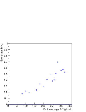
Figure 26: Event rate as function of beam energy.

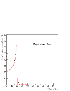
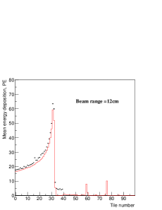
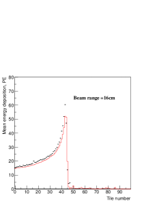
                         (a)                                     (b)                                     (c)

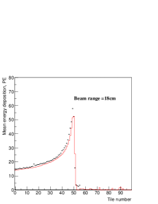
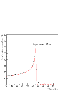
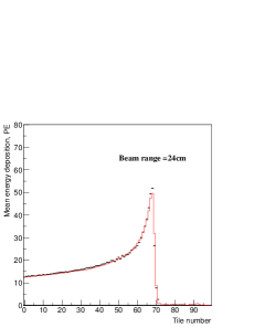
                         (d)                                     (e)                                     (f)

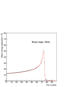
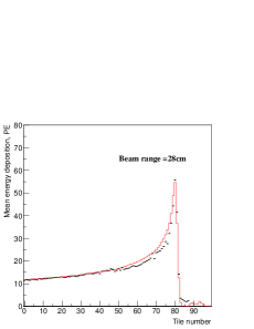
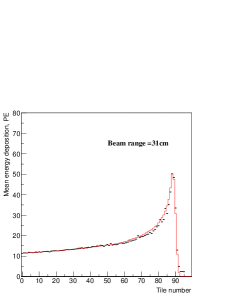
                         (g)                                     (h)                                     (i)

Figure 27: Comparison of the measured (black dots) and expected (red histograms) signal profiles in the range stack from protons of incident energy of (a) 8 cm (103 MeV); (b) 12 cm (117 MeV); (c) 16 cm (129 MeV); (d) 18 cm (162 MeV); (e) 20 cm (172 MeV); (f) 24 cm (191 MeV); (g) 26 cm (200 MeV); (h) 28 cm (208 MeV); (i) 31 cm (221 MeV).

6 Stopping range measurements in presence of a phantom

Figure 28(a) and Fig. 28(b), respectively, show the distribution of proton stopping range in the range stack and the simulated $(X,Y)$ distribution of protons at the first tracker station of the GEANT 4 detector model obtained in the presence of a spherical ($D=14~{}cm$) water phantom. The first peak in the stopping range distribution corresponds to protons going through the center of the phantom, while the second peak corresponds to the stopping range of protons that missed the phantom. Different colors for the reconstructed tracks correspond to the simulated proton stopping ranges. Figures 29(a) and (b) show similar plots for the head phantom obtained using  50K reconstructed protons of energy 200 MeV at CDH. Contours corresponding to the different material width are clearly visible. The missing bands correspond to missing tracking channels.

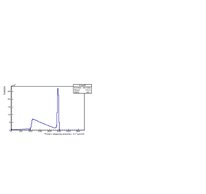
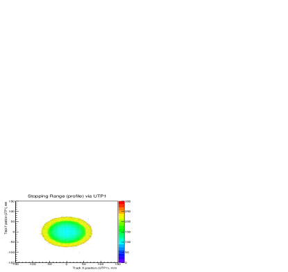
                                       (a)                                (b)

Figure 28: Water phantom (diameter of 14 cm) exposed to 300K protons of energy 200 MeV in GEANT simulations (a) the stopping range distribution (b) the stopping range profile as function of incident proton position at the first tracker station.

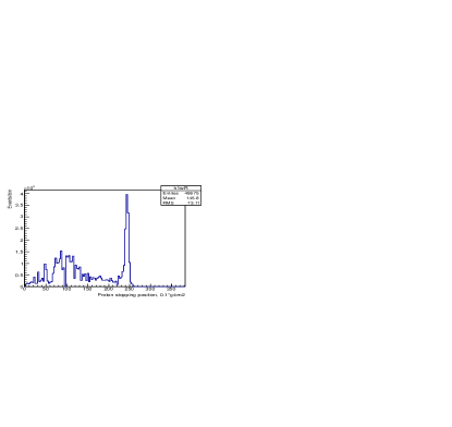
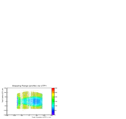
                                       (a)                                (b)

Figure 29: Head phantom exposed to  50K protons of energy 200 MeV at CDH (a) the stopping range distribution (b) the stopping range profile as a function of incident proton position at the first tracker station.

7 Summary

The stopping position measurements have better linearity and accuracy (2.2-1.2%) than the energy measurements (5.5% to 3.5%), confirmed by simulations, and thus are expected to provide more accurate WEPL calibration for the image reconstruction. The behavior of range stack detector is well modelled by GEANT, with a few dicrepancies in energy deposition at low energy and energy resolution.

References

- [1] G. Coutrakon et al., Proceedings AccApp 2013, Bruges, Belgium; S. A. Uzunyan et al., arXiv:1409.0049 (2014).
- [2] S. Uzunyan et al., Proceedings of the New Trends in High-Energy Physics, p. 152-157, Alushta, Crimea, Ukraine, Sep. 2013, ISBN 978-966-02-7015-2.
- [3] R. F. Hurleyet al., “Water-equivalent path lengh claibration of a prototype proton CT scaner”, Med. Phys. 39(5), May 2012.
- [4] J. F. Janni, ”Proton Range-Energy Tables, 1 keV-10 GeV, Energy Loss, Range, Path Length, Time-of-Flight, Straggling, Multiple Scattering, and Nuclear Interaction Probability. Part I. For 63 Compounds”, Atomic Data and Nuclear Data Tables, 27, 147, (1982).