Identifying the Optimal Integration Time in
Hamiltonian Monte Carlo

Abstract

By leveraging the natural geometry of a smooth probabilistic system, Hamiltonian Monte Carlo yields computationally efficient Markov Chain Monte Carlo estimation. At least provided that the algorithm is sufficiently well-tuned. In this paper I show how the geometric foundations of Hamiltonian Monte Carlo implicitly identify the optimal choice of these parameters, especially the integration time. I then consider the practical consequences of these principles in both existing algorithms and a new implementation called Exhaustive Hamiltonian Monte Carlo before demonstrating the utility of these ideas in some illustrative examples.

One of the most ubiquitous computational challenges in statistics is the estimation of expectations of a function with respect to a given target distribution, $\pi$. For example, we might need to compute expectations with respect to a sampling distribution in a frequentist analysis or expectations with respect to a posterior distribution in a Bayesian analysis.

Fueled by the proliferation of accessible computing resources and its applicability to many different target distributions, Markov chain Monte Carlo (Robert and Casella, 1999; Brooks et al., 2011) has become one of the most popular strategies for estimating these expectations. Here a Markov chain generated by a Markov kernel explores the target distribution, progressively building up better and better expectation estimates. Ensuring that this strategy can be scaled up to the high-dimensional and elaborate target distributions of applied interest, however, requires Markov kernels capable of efficiently exploring even the most complex distributions.

When the target distribution is smooth, Hamiltonian Monte Carlo (Duane et al., 1987; Neal, 2011; Betancourt et al., 2014) can be employed. Here the target probabilistic system is mapped into a Hamiltonian system whose canonical measure-preserving flow generates a powerful Markov transition. The ultimate performance of the resulting Markov chain, however, depends crucially on for how long we integrate along that flow: if we integrate for only a short time then the chain devolves into diffusive exploration, but long integration times offer only diminishing returns and potentially wasteful computation.

In this paper I exploit the geometry inherent to Hamiltonian Monte Carlo to isolate the relationship between integration time and effective exploration. After discussing how to implement various schemes for choosing the integration time in practice, I use this relationship to construct a natural choice of integration times known as an exhaustion and finally demonstrate the performance of the resulting exhaustive Hamiltonian Monte Carlo algorithm with some illustrative examples.

1 Hamiltonian Monte Carlo in Theory

The key to optimizing implementations of Hamiltonian Monte Carlo lies in its geometric foundations. In this section I survey the theoretical construction of the algorithm and then demonstrate how the latent microcanonical geometry naturally motivates optimality criteria.

1.1 Constructing a Generic Hamiltonian Kernel

In this paper I will consider the smooth probabilistic system $\left(Q,\mathcal{B}\!\left(Q\right),\pi\right)$, where the sample space, $Q$, is a positively-oriented and smooth $N$-dimensional manifold, $\mathcal{B}\!\left(Q\right)$ is the canonical Borel $\sigma$-algebra, and $\pi$ is a smooth probability distribution. Our ultimate goal is to compute expectations of functions $f:Q\rightarrow\mathbb{R}$ with respect to $\pi$, which we’ll approximate using Markov chain Monte Carlo estimators. The resulting computational challenge is to develop a Markov kernel that efficiently explores the target distribution, $\pi$.

Hamiltonian Monte Carlo constructs such a kernel by mapping the given probabilistic system into a Hamiltonian system (Betancourt et al., 2014). Formally, any choice of a disintegration on the cotangent bundle, $\xi\in\Xi\!\left(\varpi:T^{*}Q\rightarrow Q\right)$, immediately lifts the target distribution onto the cotangent bundle via

$$\pi_{H}=\varpi^{*}\pi\wedge\xi.$$

Denoting $\theta$ the tautological one-form on the cotangent bundle with $\Omega=\wedge_{n=1}^{N}\mathrm{d}\theta$ the corresponding symplectic volume form, we can then define the Hamiltonian,

$$H=-\log\frac{\mathrm{d}\left(\varpi^{*}\pi\wedge\xi\right)}{\mathrm{d}\Omega},$$

and the corresponding Hamiltonian system, $\left(T^{*}Q,\mathrm{d}\theta,H\right)$ (Figure 1). The critical feature of this construction is that the lifted target distribution is the canonical measure on the cotangent bundle,

$$\pi_{H}=e^{-H}\Omega;$$

consequently the lifted distribution is preserved by the canonical Hamiltonian flow, which can then be used as a basis for a Markov kernel.

Figure 1: Hamiltonian Monte Carlo maps a probabilistic system into a Hamiltonian one. Here, for example, (a) a smooth probability distribution on the circle is lifted by (b) a disintegration on the cotangent fibers to define (c) a probability distribution on the cotangent bundle. This joint distribution then canonically defines (d) a compatible Hamiltonian system.

First, however, let’s consider the local corollary of this construction. In a local neighborhood of the sample space, $\mathcal{U}_{\alpha}\subset Q$, the target distribution decomposes as

$$\pi=e^{-V}\mathrm{d}q^{1}\wedge\ldots\wedge\mathrm{d}q^{n},$$

where $V$ is known as the potential energy. Similarly, in the corresponding neighborhood of the cotangent bundle, $\varpi^{-1}\!\left(\mathcal{U}_{\alpha}\right)\subset T^{*}Q$, the smooth disintegration, $\xi$ decomposes into

$$\xi=e^{-K}\mathrm{d}p_{1}\wedge\ldots\wedge\mathrm{d}p_{n}+\text{horizontal}\;n\text{-forms},$$

with $K$ known as the kinetic energy. Locally the lift onto the cotangent bundle becomes

$$\pi_{H} =\varpi^{*}\pi\wedge\xi$$

$$=e^{-\left(V+K\right)}\mathrm{d}q^{1}\wedge\ldots\wedge\mathrm{d}q^{n}\wedge\mathrm{d}p_{1}\wedge\ldots\wedge\mathrm{d}p_{n}$$

$$=e^{-H}\Omega,$$

with the Hamiltonian

$$H=-\log\frac{\mathrm{d}\pi_{H}}{\mathrm{d}\Omega}=K+V,$$

taking a form familiar from classical mechanics (José and Saletan, 1998).

We can now use the Hamiltonian flow of this engineered Hamiltonian system to construct a powerful Markov transition. First we lift an initial point from the sample space to the cotangent bundle by sampling from the corresponding cotangent fiber,

$$p\sim\iota_{q}^{*}\xi$$

$$l :Q\rightarrow T^{*}Q$$

$$\quad q\,\mapsto\left(q,p\right)$$

$$l_{*}\pi=\pi_{H}.$$

We then apply the Hamiltonian flow for a random time depending on the initial point,

$$t \sim\pi_{T(q,p)}$$

$$\phi^{H}_{t} :T^{*}Q\rightarrow T^{*}Q$$

$$\left(\phi^{H}_{t}\right)_{*}\pi_{H}=\pi_{H},$$

and finally project back down to the sample space,

$$\varpi:T^{*}Q \rightarrow Q$$

$$\varpi_{*}\pi_{H} =\pi.$$

Composing these steps together,

$$g=\varpi\circ\phi^{H}_{t}\circ l,$$

yields a space of measure-preserving diffeomorphisms,

$$g\in \,G$$

$$g:Q \rightarrow Q$$

$$g_{*}\pi =\pi,$$

with the corresponding semi-direct product measure, $\gamma_{q}=\pi_{T(q,p)}\rtimes\iota^{*}_{q}\xi$, that immediately defines a Hamiltonian kernel as an iterated random function (Diaconis and Freedman, 1999; Quas, 1991)

$$\mathcal{T}_{\mathrm{HMC}}\!\left(q,A\right)\equiv\int_{G}\gamma_{q}\!\left(\mathrm{d}g\right)\mathbb{I}_{A}\!\left(g\left(q\right)\right),$$

where $\mathbb{I}$ is the indicator function,

$$\mathbb{I}_{A}\!\left(q\right)\propto\left\{\begin{array}[]{rr}0,&q\notin A\\ 1,&q\in A\end{array}\right.,\,q\in Q,A\in\mathcal{B}\!\left(Q\right).$$

1.2 Specifying an Optimal Hamiltonian Kernel from the Geometry of Microcanonical Systems

Unfortunately this construction is too general: every choice of cotangent disintegration, $\xi$, and distribution over integration times, $\pi_{T(q,p)}$, yields a different kernel, and the performance of these kernels can vary substantially when applied to a given target distribution. Consequently, a careful choice of kernel is critical to realizing the full potential of Hamiltonian Monte Carlo.

In this section I review how Hamiltonian systems naturally disintegrate into microcanonical systems compatible with the Hamiltonian flow. By analyzing the interaction of the Hamiltonian flow with this microcanonical geometry we can guide the construction of a unique kernel optimized to a given target distribution.

1.2.1 The Microcanonical Disintegration

One of the special properties of Hamiltonian systems is that they foliate into level sets, or submanifolds of constant energy, $E$,

$$H^{-1}\!\left(E\right)=\left\{z\in T^{*}Q\mid H\!\left(z\right)=E\right\}.$$

These level sets can be regular, in which case they contain only regular points of the Hamiltonian, or they can be critical, in which case they contain at least one critical point of the Hamiltonian. When the critical level sets are removed, the cotangent bundle decomposes into disconnected components, $T^{*}Q=\coprod_{i}M_{i}$, each of which foliates into level sets that are diffeomorphic to some common manifold (Figure 2). Consequently each $H:M_{i}\rightarrow\mathbb{R}$ becomes a smooth fiber bundle with the level sets taking the role of the fibers.

The canonical distribution restricted to each of these components then disintegrates into microcanonical distributions uniform on each level set,

$$\pi_{H^{-1}(E)}=\frac{\vec{v}\,\lrcorner\,\Omega}{\int_{H^{-1}(E)}\iota^{*}_{E}\left(\vec{v}\,\lrcorner\,\Omega\right)},$$

and a marginal energy distribution given by

$$\pi_{E}=H_{*}\pi=\frac{e^{-E}}{\int_{T^{*}Q}e^{-H}\Omega}\frac{\left(\int_{H^{-1}(E)}\iota_{E}^{*}\left(\vec{v}\,\lrcorner\,\Omega\right)\right)}{\mathrm{d}H\!\left(\vec{v}\right)}\mathrm{d}E,$$

where $\vec{v}$ is any positively-oriented horizontal vector field satisfying $\mathrm{d}H\!\left(\vec{v}\right)=c$ for some $0<c<\infty$. Because the critical level sets have zero measure with respect to the canonical distribution, the component disintegrations also define a valid disintegration of the entire cotangent bundle.

Figure 2: The foliation of a Hamiltonian system into level sets naturally defines a fiber bundle on which we can disintegrate measures. For example, once the critical level sets, here shown in red, are removed, a Hamiltonian system on the cylinder becomes a smooth fiber bundle with fiber space $F=\mathbb{S}^{1}$. Correspondingly, the canonical distribution disintegrates into microcanonical distributions uniform on each circular fiber.

The expectation of any smooth function $f:Q\rightarrow\mathbb{R}$, with respect to the target distribution, $\mathbb{E}_{\pi}\!\left[f\right]$, then decouples into expectations with respect to the microcanonical distributions nested in an expectation with respect to energies,

$$\mathbb{E}_{\pi}\!\left[f\right] =\mathbb{E}_{\pi_{H}}\!\left[f\right]$$

$$=\int_{T^{*}Q}f\,\pi_{H}$$

$$=\int_{T^{*}Q}f\pi_{E}\wedge\pi_{H^{-1}\left(E\right)}$$

$$=\int_{E}\pi_{E}\int_{H^{-1}\left(E\right)}f\,\pi_{H^{-1}\left(E\right)}.$$ (1)

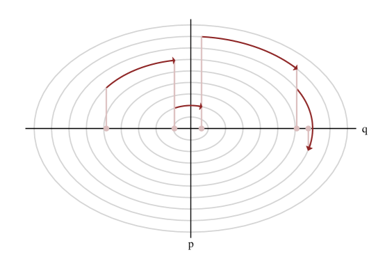
Critically, the microcanonical disintegration is compatible with the Hamiltonian flow: every Hamiltonian trajectory is confined to a single level set and, because the Hamiltonian flow restricted to a level set also preserves the corresponding microcanoncial distribution, these trajectories will explore the microcanonical distribution if integrated long enough. Consequently a Hamiltonian Markov chain decouples into a deterministic flow along levels sets, with the projection and subsequent lift, $\lambda\circ\varpi:T^{*}Q\rightarrow T^{*}Q$, resampling the momentum and inducing a random walk between level sets (Figure 3). The autocorrelation of the Markov chain then depends on both how effectively the Hamiltonian flow explores each microcanonical distribution and how effectively the momentum resampling explores the marginal energy distribution.

Figure 3: Every Hamiltonian Markov chain alternatives between a deterministic Hamiltonian flow that explores a single level set (dark red) and a momentum resampling that transitions between level sets with a random walk (light red). The longer the flow is integrated the more efficiently the Markov chain can explore each level set and the smaller the autocorrelations will be. When the flow is integrated for only an infinitesimally small time the Markov chain devolves into a Langevin diffusion.

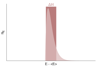
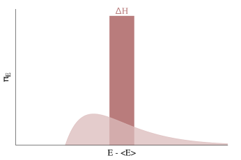
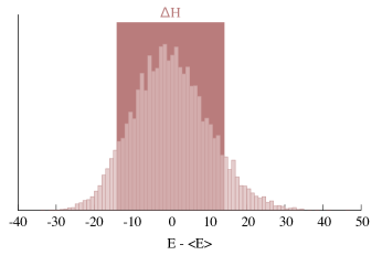
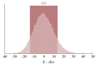
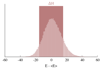
The exploration of the energy distribution depends on how much the Hamiltonian varies under a momentum resampling, $\Delta H$, relative to the width of the marginal energy distribution: the less the energy can vary in each transition the fewer level sets can be reached and the larger the autocorrelations will be (Figure 4). Because this ratio is fully determined by the interaction of the cotangent disintegration and the target distribution, it provides the foundations for the optimal choice of the cotangent disintegration itself. Formalizing this approach will be the subject of future work.

Figure 4: Every momentum resampling induces a change in the Hamiltonian, which allows a Hamiltonian Markov chain to randomly walk amongst energy level sets. (a) When the expected variation, $\Delta H$, is similar to the width of the marginal energy distribution this random walk will rapidly explore this distribution, but (b) when the expected variation is small the exploration will suffer from large autocorrelations. Optimizing the exploration of the marginal energy distribution provides an implicit criteria for selecting an optimal cotangent disintegration, and the energy autocorrelations define a constructive diagnostic for a poorly chosen cotangent disintegration.

When the cotangent disintegration is well-chosen, the performance of the resulting Markov chain is then determined by how effectively the Hamiltonian flow explores each microcanonical distribution, which in turn depends on for how long the flow is integrated along each level set. If the flow is integrated for only a short time then the transition will examine only a small neighborhood of each level set and the Markov chain will suffer from large autocorrelations. As the integration time grows the flow more completely explores each level set and reduces the autocorrelation of the chain. The additional exploration given by increasing the integration time, however, will eventually suffer from diminishing returns and ultimately not be worth the additional cost. Formalizing this intuition into a criterion for selecting an optimal compromise requires a more careful investigating of how Hamiltonian flow explores each microcanonical distributions.

1.2.2 The Ergodicity of Hamiltonian Flow

The ideal circumstance for exploration is dynamical ergodicity, where almost every trajectory eventually passes through almost every point on the corresponding level set, at least in the limit of an infinite integration time. Under these conditions the Birkhoff ergodic theorem (Petersen, 1989) states that the temporal average of any function along a trajectory converges to the the spatial average with respect to the microcanonical distribution,

$$\left<f\right>_{\phi^{H}}\!\left(z,T\right)\equiv\lim_{T\rightarrow\infty}\frac{1}{T}\int_{0}^{T}\mathrm{d}t\,f\circ\phi^{H}_{t}\!\left(z\right)=\mathbb{E}_{\pi_{H^{-1}\left(E\right)}}\!\left[f\right],$$

for $\pi_{H^{-1}\left(E\right)}$ almost all initial $z\in H^{-1}\!\left(E\right)\subset T^{*}Q$. In particular, a uniform sample from any trajectory will converge in distribution to a sample from the corresponding microcanonical distribution as the integration time grows, suggesting that we take $\pi_{T(z)}=U\!\left(0,T(z)\right)$ for some appropriating chosen $T(z)$.

Unfortunately Hamiltonian systems are not always dynamically ergodic. Depending on the topology of the level sets and the nonlinearity of the Hamiltonian, for example, trajectories may be confined to only subspaces within a level set (Hofer and Zehnder, 2011), and identifying those systems that are dynamically ergodic is challenging if not outright infeasible. The only guarantee that we have for a generic Hamiltonian system is that the time average along the flow converges to the spatial expectation along the domain of the trajectory, $\pi_{\phi^{H}(z)}$,

$$\lim_{T\rightarrow\infty}\frac{1}{T}\int_{0}^{T}\mathrm{d}t\,f\circ\phi^{H}_{t}\!\left(z\right) =\mathbb{E}_{\pi_{\phi^{H}(z)}}\!\left[f\right]$$

$$=\frac{\int_{\phi^{H}(z)}\pi_{H}f}{\int_{\phi^{H}(z)}\pi_{H}}$$

$$=\frac{\int_{\phi^{H}(z)}\pi_{H^{-1}(H(z))}f}{\int_{\phi^{H}(z)}\pi_{H^{-1}(H(z))}},$$

where the domain, $\phi^{H}\!\left(z\right)$, is also known as an orbit of the Hamiltonian flow,

$$\phi^{H}\!\left(z\right)=\left\{\phi^{H}_{t}\!\left(z\right),\forall t\in\mathbb{R}\right\}\subset H^{-1}\!\left(H\!\left(z\right)\right).$$

Although the trajectory may not explore the entire level set, it will at least explore the entire orbit, and a uniform sample from the trajectory will converge in distribution to a sample from $\pi_{\phi^{H}(z)}$ as the integration time grows.

Even though integrating for ever longer times will improve convergence, yielding more accurate samples and reducing the autocorrelations of the resulting Hamiltonian Markov chain, longer integration times may not be worth the additional cost. When the integration time is small and the trajectory is just beginning to explore its orbit, for example, the convergence to the corresponding spatial expectation can be superlinear, justifying the linear cost of increasing the integration time. For long integration times, however, the temporal expectations typically converge with only the square root of the integration time (Cancès et al., 2005), and the cost of additional integration begins to undermine the performance of the chain (Figure 5).

Figure 5: (a) Temporal averages along a Hamiltonian trajectory converge to the corresponding spatial expectation, $\pi_{\phi^{H}(z)}$, as the integration time grows, (b) inducing convergence of any Monte Carlo estimator, here represented by the number of effective samples per transition. Typically this convergence is initially rapid and superlinear before settling into an asymptotic regime where the convergence continues only with the square of the integration time. (c) Because cost of simulating each trajectory scales with the integration time, those integration times, $T\!\left(z\right)$, that identify the transition between these two regimes uniformly for all $z\in T^{*}Q$, yields optimal performance.

Consequently, optimal performance requires identifying a maximal integration time for each trajectory, $T\!\left(z\right)$, with the resulting uniform measure, $\pi_{T(z)}=U\!\left(0,T(z)\right)$, that identifies the transition between these two regimes uniformly across all level sets. Intuitively this transition should occur after the trajectory has first traversed the extent of its orbit (Figure 6a), with the asymptotic behavior corresponding to the trajectory exploring finer and finer details of the orbit (Figure 6b). Formalizing this intuition into an explicit optimization criterion, however, is not straightforward.

Figure 6: (a) Intuitively, the temporal average along a Hamiltonian trajectory rapidly converges to the spatial expectation over its orbit as the trajectory first spans the orbit. (b) Longer trajectories simply refine this initial exploration, yielding better but slower convergence.

1.2.3 Poincaré Recurrence and Autocorrelation Functions

One natural strategy for identifying optimal integration times is to appeal to Poincaré recurrence. If the Hamiltonian is proper and its level sets compact (Lee, 2011) then all Hamiltonian orbits will be bounded and the Poincaré recurrence theorem (Zaslavsky, 2008) states that the trajectories originating from almost any point will explore the corresponding orbit and then return to any neighborhood of that point within some finite recurrence time (Figure 7).

Figure 7: When its orbit is compact, (a) a Hamiltonian trajectory (b) will return to any neighborhood of almost every initial point within some finite recurrence time. (c) The smaller the neighborhood, the longer the recurrence time, and the more thoroughly the trajectory will explore its orbit and converge to the corresponding spatial expectation.

The recurrence corresponding to well-behaved neighborhoods then immediately formalizes and implements our above intuitions. At least it would if we could define the necessary behavior and then explicitly define the corresponding neighborhoods and identify recurrence exactly. Unfortunately none of these are particularly practical for most Hamiltonian systems.

An alternative strategy that is both general and easily implemented, if less inspired, is to use an auxiliary autocorrelation function,

$$\kappa\!\left(T,z\right)=\kappa\!\left(\phi^{H}_{T}\!\left(z\right),z\right),$$

that monotonically converges to zero for all initial initial points,

$$\lim_{T\rightarrow\infty}\left|\kappa\!\left(T,z\right)\right|=0,\,\forall z\in T^{*}Q.$$

Relaxing this to a uniform bound gives an termination criterion,

$$\left|\kappa\!\left(T,z\right)\right|\leq\delta,\delta\in\mathbb{R}^{+},$$ (2)

which implicitly defines a set of integration times,

$$T_{\kappa}\!\left(z\right)=\min\left\{t\mid\left|\kappa\!\left(t,z\right)\right|\leq\delta\right\},$$

with $\delta$ providing some control over the amount of convergence. If $\kappa\!\left(T,z\right)$ is not monotonic, for example if it oscillates around zero, then this interpretation becomes more complicated; although this is not ideal, the resulting integration times may still provide some uniformity of exploration over each level set and hence identify useful integration times.

Additionally, these two strategies are not mutually exclusive. Because there always exists a compact neighborhood containing $z$ with $\phi^{H}_{T_{\kappa}(z)}$ on its boundary, when the level sets are compact $T_{\kappa}(z)$ can always be interpreted as a recurrence time for some implicit recurrence neighborhood. Consequently, for some geometries Poincaré recurrence may be useful in motivating useful autocorrelation functions

2 Hamiltonian Monte Carlo in Practice

Regardless of how a Hamiltonian kernel is chosen, any implementation of the underlying Hamiltonian flow requires solving a system of $2n$ first-order ordinary differential equations. For all but the simplest systems analytical solutions are unfeasible and we must instead resort to simulating the flow numerically. Fortunately, there exist a family of numerical integrators that employ the underlying symplectic geometry to conserve many of the properties of the exact flow (Hairer, Lubich and Wanner, 2006; Leimkuhler and Reich, 2004). These symplectic integrators exactly preserve the symplectic volume form with only small variations in the Hamiltonian along the simulated flow.

In fact, symplectic integrators simulate some flow exactly, just not the flow corresponding to $H$. Backwards error analysis shows that the discrete time steps of a $k$-th order symmetric symplectic integrator exactly fall onto the flow for some modified Hamiltonian, given by an even, asymptotic expansion with respect to the integrator step size, $\epsilon$,

$$\widetilde{H}=H+\sum_{n=k/2}^{N}\epsilon^{2n}H_{\left(n\right)}+\mathcal{O}\!\left(e^{-c/\epsilon}\right).$$

Because it is exponentially small in the step size, the asymptotic error is typically neglected and the leading-order behavior of the modified Hamiltonian is given by

$$\widetilde{H}=H+\epsilon^{k}G+\mathcal{O}(\epsilon^{k+2}).$$

This discretized, approximate flow then generates a series of states,

$$z_{L}\equiv\Phi^{\widetilde{H}}_{\epsilon,L\cdot\epsilon}(z_{0})\in T^{*}Q,\,L\in\mathbb{Z},$$

that tracks the true flow for exponentially long times. The symplectic integrator will still introduce some error, however, and, while that error can be managed by the choice of step size, it will still bias the resulting Markov chain if left uncorrected. Correcting this error is a delicate problem that depends crucially on how the numerical trajectories are used, and hence the distribution of integration times, $\pi_{T(z)}$.

2.1 Static Implementations

The simplest implementation of Hamiltonian Monte Carlo uses a single, static integration time, $T\!\left(z\right)=T$, or, equivalently, a static number of symplectic integrator steps, $L=T/\epsilon$.

When using only the final point of each trajectory, in other words taking a Dirac measure on integration times, $\pi_{T(z)}=\delta_{L\cdot\epsilon}$, we might naively consider treating the numerical trajectory as a Metropolis proposal, accepting the final state with only probability,

$$a\!\left(z_{0},z_{L}\right) =\min\!\left[1,\frac{\mathrm{d}\pi_{H}}{\mathrm{d}\Omega}\!\left(z_{L}\right)\frac{\mathrm{d}\Omega}{\mathrm{d}\pi_{H}}\!\left(z_{0}\right)\right]$$

$$=\min\!\left[1,\exp\!\left(H\!\left(z_{L}\right)-H\!\left(z_{0}\right)\right)\right].$$

Unfortunately the non-reversible nature of the flow renders it an invalid Metropolis proposal unless augmented.

The numerical trajectory becomes a valid Metropolis proposal only when manipulated into an involution (Tierney, 1998), for example, by composing the flow with any operator, $R$, satisfying

$$\Phi^{\tilde{H}}_{\epsilon,L\cdot\epsilon}\circ R\circ\Phi^{\tilde{H}}_{\epsilon,L\cdot\epsilon}=\mathrm{Id}_{T^{*}Q}.$$

The probability of accepting the final state is then given by

$$a\!\left(z_{0},R\!\left(z_{L}\right)\right) =\min\!\left[1,\frac{\mathrm{d}\pi_{H}}{\mathrm{d}\Omega}\!\left(R\!\left(z_{L}\right)\right)\frac{\mathrm{d}\Omega}{\mathrm{d}\pi_{H}}\!\left(z_{0}\right)\right]$$

$$=\min\!\left[1,\exp\!\left(H\circ R\circ\!\left(z_{L}\right)-H\!\left(z_{0}\right)\right)\right].$$

Our analysis of the microcanonical geometry, however, motivated not a Dirac measure on integration times but rather sampling uniformly from the entire trajectory, $\pi_{T}=U\!\left(0,T\right)$. Unfortunately, sampling from a numerical trajectory while also correcting for the error in the symplectic integrator is a not straightforward given that Metropolis sampling from states generated by integrating only forwards in time breaks detailed balance (Figure 8),

$$\mathbb{P}\!\left[z_{l}\mid z_{0}\right]\frac{\mathrm{d}\pi_{H}}{\mathrm{d}\Omega}\!\left(z_{0}\right) =\frac{\frac{\mathrm{d}\pi_{H}}{\mathrm{d}\Omega}\!\left(z_{l}\right)\frac{\mathrm{d}\pi_{H}}{\mathrm{d}\Omega}\!\left(z_{0}\right)}{\sum_{m=0}^{L}\frac{\mathrm{d}\pi_{H}}{\mathrm{d}\Omega}\!\left(z_{m}\right)}$$

$$\mathbb{P}\!\left[z_{0}\mid z_{l}\right]\frac{\mathrm{d}\pi_{H}}{\mathrm{d}\Omega}\!\left(z_{l}\right) =0,$$

and obstructs the invariance of the target distribution.

Figure 8: If numerical trajectories are generated by integrating only forwards in time then a state cannot be sampled from the entire trajectory without destroying the invariance of the target distribution. Sampling from trajectories while maintaining the correct invariant distribution requires considering trajectories that integrate both forwards and backwards in time from the initial state, $z_{0}$.

In order to guarantee detailed balance and hence maintain the invariance of the target distribution, we need to consider not just those numerical trajectories that begin at the initial point but also those trajectories that only contain the initial point. Defining $\mathfrak{T}_{z,L}$ as the set of all numerical trajectories of length $L$ that contains the state $z$, we need to consider transitions that first sample a trajectory $\mathfrak{t}\in\mathfrak{T}_{z_{0},L}$, with probability $\mathbb{P}\!\left[\mathfrak{t}|z_{0}\right]$ and then sample a state from that trajectory with probabilities $\mathbb{P}\!\left[z|\mathfrak{t}\right]$.

Provided that the states within each trajectory are appropriately weighted with the Metropolis probabilities,

$$\mathbb{P}\!\left[z|\mathfrak{t}\right]=\frac{\frac{\mathrm{d}\pi_{H}}{\mathrm{d}\Omega}\!\left(z\right)}{\sum_{z^{\prime}\in\mathfrak{t}}\frac{\mathrm{d}\pi_{H}}{\mathrm{d}\Omega}\!\left(z^{\prime}\right)}=\frac{e^{-H(z)}}{\sum_{z^{\prime}\in\mathfrak{t}}e^{-H(z^{\prime})}},$$ (3)

then the equality of trajectory probabilities,

$$\mathbb{P}\!\left[\mathfrak{t}|z_{1}\right]=\mathbb{P}\!\left[\mathfrak{t}|z_{2}\right],\,\forall\mathfrak{t}\in\mathfrak{T}_{z_{1},L}\cap\mathfrak{T}_{z_{2},L}\equiv\mathfrak{T}_{(z_{1},z_{2}),L},$$ (4)

is sufficient to ensure detailed balance,

$$\mathbb{P}\!\left[z_{1}|z_{2}\right]\frac{\mathrm{d}\pi_{H}}{\mathrm{d}\Omega}\!\left(z_{2}\right) =\sum_{\mathfrak{t}\in\mathfrak{T}_{(z_{1},z_{2}),L}}\mathbb{P}\!\left[z_{1}|\mathfrak{t}\right]\mathbb{P}\!\left[\mathfrak{t}|z_{2}\right]\frac{\mathrm{d}\pi_{H}}{\mathrm{d}\Omega}\!\left(z_{2}\right)$$

$$=\sum_{\mathfrak{t}\in\mathfrak{T}_{(z_{1},z_{2}),L}}\frac{\frac{\mathrm{d}\pi_{H}}{\mathrm{d}\Omega}\!\left(z_{1}\right)}{\sum_{z^{\prime}\in\mathfrak{t}}\frac{\mathrm{d}\pi_{H}}{\mathrm{d}\Omega}\!\left(z^{\prime}\right)}\mathbb{P}\!\left[\mathfrak{t}|z_{2}\right]\frac{\mathrm{d}\pi_{H}}{\mathrm{d}\Omega}\!\left(z_{2}\right)$$

$$=\left(\sum_{\mathfrak{t}\in\mathfrak{T}_{(z_{1},z_{2}),L}}\frac{\frac{\mathrm{d}\pi_{H}}{\mathrm{d}\Omega}\!\left(z_{2}\right)}{\sum_{z^{\prime}\in\mathfrak{t}}\frac{\mathrm{d}\pi_{H}}{\mathrm{d}\Omega}\!\left(z^{\prime}\right)}\mathbb{P}\!\left[\mathfrak{t}|z_{2}\right]\right)\frac{\mathrm{d}\pi_{H}}{\mathrm{d}\Omega}\!\left(z_{1}\right)$$

$$=\left(\sum_{\mathfrak{t}\in\mathfrak{T}_{(z_{1},z_{2}),L}}\frac{\frac{\mathrm{d}\pi_{H}}{\mathrm{d}\Omega}\!\left(z_{2}\right)}{\sum_{z^{\prime}\in\mathfrak{t}}\frac{\mathrm{d}\pi_{H}}{\mathrm{d}\Omega}\!\left(z^{\prime}\right)}\mathbb{P}\!\left[\mathfrak{t}|z_{1}\right]\right)\frac{\mathrm{d}\pi_{H}}{\mathrm{d}\Omega}\!\left(z_{1}\right)$$

$$=\left(\sum_{\mathfrak{t}\in\mathfrak{T}_{(z_{1},z_{2}),L}}\mathbb{P}\!\left[z_{2}|\mathfrak{t}\right]\mathbb{P}\!\left[\mathfrak{t}|z_{1}\right]\right)\frac{\mathrm{d}\pi_{H}}{\mathrm{d}\Omega}\!\left(z_{1}\right)$$

$$=\mathbb{P}\!\left[z_{2}|z_{1}\right]\frac{\mathrm{d}\pi_{H}}{\mathrm{d}\Omega}\!\left(z_{1}\right).$$

There are various methods for appropriately weighting the states in a numerical trajectory according to (3). For example, we could simply sample from the multinomial distribution defined by the Metropolis probabilities directly, or even apply a slice sampler that first samples $u\sim U\!\left(0,1\right)$ and then uniformly samples from those points on the trajectory satisfying

$$\frac{e^{-H(z)}}{\sum_{z^{\prime}\in\mathfrak{t}}e^{-H(z^{\prime})}}>u.$$

Designing a transition from an initial state to a numerical trajectory satisfying (4) is a more subtle challenge.

One immediate solution is to simply sample trajectories in $\mathfrak{T}_{z_{0},L}$ uniformly,

$$\mathbb{P}\!\left[\mathfrak{t}|z_{0}\right] =\left\{\begin{array}[]{rr}0,&\mathfrak{t}\notin\mathfrak{T}_{z_{0},L}\\ 1/\left|\mathfrak{T}_{z_{0},L}\right|,&\mathfrak{t}\in\mathfrak{T}_{z_{0},L}\end{array}\right.$$

$$=\left\{\begin{array}[]{rr}0,&\mathfrak{t}\notin\mathfrak{T}_{z_{0},L}\\ \hskip 25.60747pt1/L,&\mathfrak{t}\in\mathfrak{T}_{z_{0},L}\end{array}\right..$$

Because each trajectory is equally likely regardless of the initial point, (4) holds trivially (Figure 9). Moreover, sampling trajectories uniformly is straightforward to implement, for example by sampling $L^{\prime}\sim U\!\left[0,L\right]$ and integrating backwards for $L^{\prime}$ steps and forwards for $L-L^{\prime}$ steps. When sampling a final state using the Metropolis probabilities directly, this is equivalent to Neal’s Windowed State Algorithm with $W=L$ (Neal, 1994).

Figure 9: By uniformly sampling all numerical trajectories in $\mathfrak{T}_{z,L}$ regardless of the initial $z$, we ensure that $\mathbb{P}\!\left[\mathfrak{t}|z\right]=1/L,\forall z\in\mathfrak{t}$, which immediate guarantees (4) and hence detailed balance of the resulting Markov chain.

Still, all of this effort lets us uniformly sample only from static trajectories of constant length, $L$, and not the dynamic trajectories capable of expanding to ensure uniform exploration of the underlying level sets. Sampling from trajectories that integrate for a dynamic number of steps determined by a termination criterion such as (2) requires a careful extension of the static implementation.

2.2 Dynamic Implementations

In order to maintain a uniform distribution over numerical trajectories when their length, $L$, is dynamic we have to build up each trajectory incrementally, checking if a termination criterion like (1.2.3) has been satisfied after each expansion (Algorithm 1). For example, a uniformly sampled trajectory can be build up additively by iteratively expanding the trajectory one step at a time in a random direction (Figure 10a). If we consider trajectories of only lengths $2^{D}$ then we can also build up uniformly sampled trajectories multiplicatively, expanding a trajectory of length $L$ by integrating $L$ additional steps in a random direction (Figure 10b). In this multiplicative scheme each intermediate trajectory can also be interpreted as a balanced binary tree (Figures 11, 12).

Algorithm 1 Given a means to expand a trajectory, such as the additive or multiplicative schemes discussed in the text, and a termination criterion that implicitly identifies the optimal integration time, a uniformly sampled trajectory can be built up recursively.

function expand_trajectory($\mathfrak{t}$)

function check_termination($\mathfrak{t}$)

function naive_build_trajectory($\mathfrak{t}$)

     $\mathfrak{t}_{\mathrm{new}}\leftarrow$ expand_trajectory($\mathfrak{t}$)

     if  check_termination($\mathfrak{t}_{\mathrm{new}}$)  then

         return $\mathfrak{t}_{\mathrm{new}}$

     else

         naive_build_trajectory($\mathfrak{t}_{\mathrm{new}}$)      

Figure 10: Uniformly sampling numerical trajectories of a dynamic length requires that the trajectories are generated incrementally. Trajectories can be generated recursively, either with (a) additive increments that randomly integrate the trajectory forwards or backward a single step or (b) multiplicative increments that double a trajectory of length $L$ by randomly integrating forward or backwards $L$ additional steps.

Figure 11: A numerical trajectory of length $L=2^{D}$ can be represented as the leaves of a perfect, ordered binary tree of depth $D$. The initial and final points of the trajectory, labeled $z_{-}$ and $z_{+}$ respectively, serve as the tree boundaries.

Figure 12: In the tree representation, a multiplicative expansion of a numerical trajectory of length $L=2^{D}$ is given by randomly selecting a boundary, here $z_{+}$, and integrating away from the tree $L$ additional steps. This process can also be considered as appending (b) a new tree of depth $D$ to (a) the original tree of depth $D$ to give (c) an expanded tree of depth $D+1$.

Unfortunately, when the length is chosen dynamically uniformly sampling trajectories is no longer sufficient to ensure (4), as different initial states may lead to different terminal lengths (Figure 13). In order to guarantee detailed balance we have to treat each increment as a proposal, rejecting any extensions which include states from which $\mathbb{P}\!\left[\mathfrak{t}_{\mathrm{new}}|z\right]=0$ (Algorithm 2). When the trajectory length is limited by a failed proposal the resulting trajectory will not satisfy the termination criterion exactly, a price we have to pay to ensure uniform samples that target the correct distribution.

Figure 13: Uniformly sampling a numerical trajectory around the initial state, $z_{0}$, is not suffient to ensure detailed balance when the trajectory length is dynamic. The problem is that if the termination criterion is satisfied in the interior of the trajectory, here between $z_{-}^{\prime}$ and $z_{+}^{\prime}$ then both $\mathbb{P}\!\left[\mathfrak{t}|z_{-}^{\prime}\right]=0$ and $\mathbb{P}\!\left[\mathfrak{t}|z_{+}^{\prime}\right]=0$ despite $\mathbb{P}\!\left[\mathfrak{t}|z_{0}\right]\neq 0$.

Algorithm 2 Ensuring detailed balance with dynamic trajectories requires not just uniformly sampling a trajectory for an initial point, but also ensuring that the final trajectory can be reached from all points in that trajectory. Given a means of validating each intermediate trajectory the final algorithm is a straightforward modification of Algorithm 1.

function expand_trajectory($\mathfrak{t}$)

function validate_trajectory($\mathfrak{t}$)

function check_termination($\mathfrak{t}$)

function build_trajectory($\mathfrak{t}$)

     $\mathfrak{t}_{\mathrm{new}}\leftarrow$ expand_trajectory($\mathfrak{t}$)

     if validate_trajectory($\mathfrak{t}_{\mathrm{new}}$)  then

         if  check_termination($\mathfrak{t}_{\mathrm{new}}$)  then

              return $\mathfrak{t}_{\mathrm{new}}$

         else

              naive_build_trajectory($\mathfrak{t}_{\mathrm{new}}$)          

     else

         return $\mathfrak{t}$      

How a given trajectory is validated to ensure that there are no states with $\mathbb{P}\!\left[\mathfrak{t}_{\mathrm{new}}|z\right]=0$ depends on the expansion method. Additive expansions, for example, require that the termination criterion not be satisfied for every pair of states in the trajectory. If checked recursively, this requires $L$ checks after proposing a new trajectory of length $L$, as well as the local storage of each state in the trajectory. Multiplicative expansions have the advantage that the termination criterion needs to be checked for only the subtrees (Figure 14), requiring only $\log(L)$ checks for a proposed trajectory of length $L$ and only $\log(L)$ states in memory at any given time.

Figure 14: Ensuring detailed balance requires validating each trajectory expansion before accepting the new trajectory. For multiplicative expansion this requires that no internal subtree of the proposal satisfies the termination criterion. (a) If no subtree satisfies the termination criterion then it can appended to the trajectory, resulting in an expanded trajectory that can then be checked for termination and further expanded as necessary. (b) Conversely, when a subtree does satisfy the termination criterion then the proposal must be rejected and the trajectory construction immediately terminated.

2.3 Alternative Schemes

Before considering explicit termination criteria, let us briefly pause to discuss alternative schemes for constructing Markov chains using Hamiltonian flow. Ultimately, the cause of poor performance when using a poorly chosen integration time is the momentum resampling induced by the projection and lifting needed to map from the cotangent bundle down to the target space and back. Constructing a Markov chain on the cotangent bundle directly, however, could invalidate the need for the momentum resampling and conceivably yield improved performance even with a suboptimal integration time.

The Horowitz scheme (Horowitz, 1991), for example, uses Hamiltonian flow mixed with only partial momentum resampling to move between the level sets. After integrating for the prescribed integration time, a Metropolis correction is applied: if the state is accepted then the final momentum is mixed with newly sampled momenta, maintaining some coherency in the exploration. The cost of this approach, however, is that in order to preserve the target distribution the momentum must be completely negated after a rejection, causing the next trajectory to return to a neighborhood that has already been explored. Extra-chance schemes (Sohl-Dickstein, Mudigonda and DeWeese, 2014; Campos and Sanz-Serna, 2015) take this idea even further, applying a fixed number of proposals which do not modify the momentum at all after an acceptance while continuing to negate after rejections to ensure the correct stationary distribution.

Both schemes, however, can maintain the coherency of the exploration only while the symplectic integrator is near the true flow, devolving into diffusive exploration as the symplectic integrator strays and the proposals are rejected. Optimal performance is then achieved when the total integration time, for one proposal in a Horowitz scheme or the many proposals of an extra-chance scheme, is matched to the first excursion of the symplectic integrator. This almost always results in premature termination, however, as the volume preservation of the symplectic integrator ensures that it does not drift and that these excursions are only temporary (Figure 15). To truly exploit the exploratory power of Hamiltonian flow with symplectic integrators, we need to be able integrate far past these temporary excursions.

Figure 15: Because they are volume preserving, symplectic integrators do not drift from the true Hamiltonian flow even over exponentially long integration times. The numerical trajectory effectively oscillates near the true trajectory, and any increasing error is only temporary.

3 Explicit Termination Criteria

Now that we know how to implement Hamiltonian Monte Carlo with dynamic integration times we just need to select an explicit termination criterion capable of identifying optimal, or at least approximately optimal, integration times. Fortunately, the underlying geometry proves ever fruitful, naturally motivating a canonical autocorrelation function that yields a set of integration times known as an exhaustion. After constructing these objects for both exact and numerical trajectories I also consider termination criteria that arise naturally when the target space is equipped with a Riemannian metric.

3.1 Theoretical Exhaustions

A particularly natural way to define autocorrelation functions on a Hamiltonian system is through the temporal expectation of the temporal derivative of any scalar function, $u$,

$$\kappa_{u}\!\left(T,z\right)\equiv\frac{1}{T}\int_{0}^{T}\mathrm{d}t\,\frac{\mathrm{d}u}{\mathrm{d}t}\circ\phi^{H}_{t}\!\left(z\right)=\frac{u\circ\phi^{H}_{T}\!\left(z\right)-u\!\left(z\right)}{T}.$$

Provided that the scalar function is bounded,

$$\left|u\circ\phi^{H}_{t}\!\left(z\right)-u\!\left(z\right)\right|<\infty,\,\forall t\in\mathbb{R},$$

then every such expectation vanishes asymptotically,

$$\lim_{t\rightarrow\infty}\kappa_{u}\!\left(t,z\right)=\lim_{t\rightarrow\infty}\frac{u\circ\phi^{H}_{t}\!\left(z\right)-u\!\left(z\right)}{t}=0,$$

making it a potential termination criterion. Care must be taken, however, as the scalar function may recur, $u\circ\phi^{H}_{t}\!\left(z\right)=u\!\left(z\right)$, preventing $\kappa_{u}$ from being monotonic and possibly resulting in premature integration times.

There aren’t many scalar functions available to construct such an autocorrelation function for a generic Hamiltonian system. One canonical scalar function is the Hamiltonian itself, but, because the Hamiltonian is conserved by the Hamiltonian flow, its time rate of change vanishes trivially making it unsuitable for tracking convergence. The only other scalar function canonical to a general Hamiltonian system is the virial, $G=q^{i}p_{i}$. When the Hamiltonian is proper and all trajectories bounded, the virial itself is always bounded and provides a potential candidate.

Collecting the resulting integration times together defines an exhaustion.

Definition 1.

An exhaustion, $T_{\delta}\!\left(z\right)$, is the family of integration times at each point in the cotangent bundle such that the temporal average of the rate of change of the virial along the resulting Hamiltonian flow is uniformly bounded,

$$\left|\frac{1}{T_{\delta}}\int_{0}^{T_{\delta}}\mathrm{d}t\,\frac{\mathrm{d}G}{\mathrm{d}t}\circ\phi^{H}_{t}\!\left(z\right)\right|=\left|\frac{G\circ\phi^{H}_{T_{\delta}}\!\left(z\right)-G\!\left(z\right)}{T_{\delta}}\right|<\delta,\,\forall z\in T^{*}Q.$$

Provided that the Hamiltonian is proper a valid exhaustion can always be constructed.

Although exhaustions are canonical to any Hamiltonian system, they will not, in general, identify optimal integration times for any choice of $\delta$. The real utility of an exhaustive termination criterion is that it ensures uniform convergence across all level sets and reduces the tuning problem to the single exhaustion threshold, $\delta$. How to identify an optimal threshold for a given problem remains an open problem.

3.2 Numerical Exhaustions

Because the exact flow is approximated with a symplectic integrator, exhaustions defined using exact expectations are not quite applicable to any practical implementation of Hamiltonian Monte Carlo. Instead we can replace the exact expectation with a Metropolis-corrected expectation over the numerical trajectory,

$$\frac{1}{\left|\mathfrak{t}\right|}\sum_{z\in\mathfrak{t}}\mathbb{P}\!\left[z|\mathfrak{t}\right]\frac{\mathrm{d}G}{\mathrm{d}t}\!\left(z\right),$$

with

$$\mathbb{P}\!\left[z|\mathfrak{t}\right]=\frac{\frac{\mathrm{d}\pi_{H}}{\mathrm{d}\Omega}\!\left(z\right)}{\sum_{z^{\prime}\in\mathfrak{t}}\frac{\mathrm{d}\pi_{H}}{\mathrm{d}\Omega}\!\left(z^{\prime}\right)}=\frac{e^{-H(z)}}{\sum_{z^{\prime}\in\mathfrak{t}}e^{-H(z^{\prime})}}.$$

Because this expectation converges to the continuous expectation in the limit of infinite steps,

$$\lim_{\left|\mathfrak{k}\right|\rightarrow\infty}\frac{1}{\left|\mathfrak{t}\right|}\sum_{z\in\mathfrak{t}}\mathbb{P}\!\left[z|\mathfrak{t}\right]\frac{\mathrm{d}G}{\mathrm{d}t}\!\left(z\right)=\lim_{T\rightarrow\infty}\frac{1}{T}\int^{T}_{0}\mathrm{d}t\,\frac{\mathrm{d}G}{\mathrm{d}t}\circ\phi^{H}_{t}\!\left(z\right)=0,$$

the numerical expectation will converge to the true expectation and provide similar termination behavior. Hence we can define an equivalent numerical exhaustion.

Definition 2.

A numerical exhaustion, $\mathfrak{T}_{\delta}$, is the set of numerical trajectories such that the Metropolis-corrected expectation of the rate of change of the virial along any element, $\mathfrak{t}$ is uniformly bounded,

$$\left|\frac{1}{\left|\mathfrak{t}\right|}\sum_{z\in\mathfrak{t}}\mathbb{P}\!\left[z|\mathfrak{t}\right]\frac{\mathrm{d}G}{\mathrm{d}t}\!\left(z\right)\right|<\delta.$$

As in the exact case, the modified Hamiltonian foliates the manifold and we can define corresponding modified level sets,

$$\widetilde{H}^{-1}\!\left(E\right)=\left\{q,p\in M\,|\,\widetilde{H}\!\left(q,p\right)=E\right\}.$$

Provided that the asymptotic error is negligible and the symplectic integrator is topologically stable (McLachlan, Perlmutter and Quispel, 2004), the modified level sets will have the same topology as the exact level sets. In particular, when the exact Hamiltonian is proper and its level sets compact, then negligible asymptotic error and topological stability imply that the modified Hamiltonian is also proper and its level sets also compact. Consequently the virial remains bounded on the numerical trajectories and the Poincaré recurrence theorem still applies, guaranteeing that numerical exhaustions are nonempty. When the topological stability and negligible asymptotic error do not hold, the numerical trajectories will rapidly diverge; these numerical divergences then serve as immediate diagnostics of an ill-posed numerical exhaustion.

Hence we can define a trajectory termination criterion by checking if $\mathfrak{t}\in\mathfrak{T}_{\delta}$, with the resulting implementation of Hamiltonian Monte Carlo denoted Exhaustive Hamiltonian Monte Carlo.

3.3 Riemannian Termination Criteria

Although the virial is the only candidate scalar function canonical to every Hamiltonian system, there are additional candidates once we endow the sample space with additional structure, such as a Riemannian metric. In particular, a Riemannian metric, $g$, allows us to define an entire family of disintegrations given in local coordinates by the kinetic energy

$$K\!\left(q,p\right)=A\cdot f\!\left(g^{-1}_{q}\!\left(p,p\right)\right)+\frac{1}{2}\log\left|g_{q}\right|+\mathrm{const},$$

for some constant $A$ and function $f:\mathbb{R}\rightarrow\mathbb{R}$. Given such a Riemannian disintegration we can then define two new scalars: the effective potential energy,

$$\widecheck{V}\!\left(q\right)=V\!\left(q\right)+\frac{1}{2}\log\left|g_{q}\right|+\mathrm{const}.$$

and the effective kinetic energy,

$$\widecheck{K}\!\left(q,p\right)=A\cdot f\!\left(g^{-1}_{q}\!\left(p,p\right)\right).$$

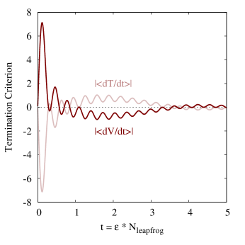
Because the Hamiltonian is conserved, the autocorrelation functions induced by these two functions are simply negations of each other and the resulting integration times identical. The difficulty with these functions is that they recur quickly, long before any reasonable recurrence of the trajectory. More formally, if the disintegration is Gaussian then the functions will recur at turning points of the orbits (Hofer and Zehnder, 2011), which are rampant in the Hamiltonian systems resulting from strongly-correlated target distributions.

A Riemannian metric also admits the construction of a completely different termination criterion. Instead of considering the temporal expectation of a scalar function we can appeal to the generalized No-U-Turn criterion (Betancourt, 2013), which terminates when

$$\kappa_{\mathrm{NUTS}}\!\left(T\right)=g^{-1}_{q}\!\left(p,\rho_{T}\right)<0$$

where

$$\rho_{T}=\frac{1}{T}\int_{0}^{T}\mathrm{d}t\,\left(\phi^{H}_{t}\right)_{*}\theta.$$

Note that when the metric is Euclidean the generalized No-U-Turn criterion reduces to the usual No-U-Turn criterion (Hoffman and Gelman, 2014). In fact, the use of the No-U-Turn criterion with multiplicative trajectory expansion and a slice sampler to draw a state from the final trajectory is exactly Hoffman and Gelman’s No-U-Turn sampler.

For simple level set geometries the generalized No-U-Turn criterion is satisfied when a trajectory has traveled from one side of a level set to to the other, matching of the intuition we developed for an optimal integration time in Section 1.2.2. Although there is no guarantee that the generalized No-U-Turn criterion always identifies the optimal integration time, its impressive empirically success suggests that it applies even in when targeting complex distributions.

One weakness that has arisen in some applications is that, because the criterion is always small in a neighborhood around the initial point, small oscillations in a trajectory can cause the criterion to vanish prematurely. Additionally, evaluating the No-U-Turn criterion is more computationally expensive than checking a numerical exhaustion, especially in the general Riemannian case.

4 Experiments

In this section I present a series of illustrative experiments to corroborate the theory and intuition developed above. I begin first with a graphical study of the exhaustive termination criteria and then follow with performance studies of various Hamiltonian Monte Carlo implementations targeting various distributions.

4.1 Graphical Experiments

To illuminate the qualitative behavior of the exhaustive termination criterion relative to the No-U-Turn criterion, consider a two-dimensional Gaussian distribution with a Euclidean-Gaussian disintegration, given in local coordinates by the effective potential energy

$$\widecheck{V}\!\left(q\right)=\frac{1}{2}q^{i}q^{j}\frac{\delta_{ij}-\left(1-\delta_{ij}\right)\rho}{1-\rho^{2}}+\mathrm{const}$$

and the effective kinetic energy

$$\widecheck{K}\!\left(q,p\right)=\frac{1}{2}p_{i}p_{j}\delta^{ij},$$

where $\delta_{ij}$ is the discrete Dirac-delta function not to be confused with the exhaustive termination threshold, $\delta$.

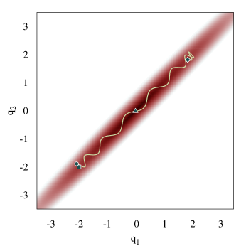
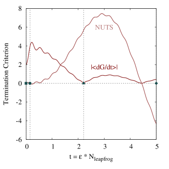
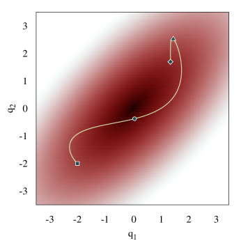
For $\rho=0.99$ the target distribution is highly correlated (Figure 16a). The strong correlations induce premature termination of the No-U-Turn criterion but the exhaustive termination criterion yields substantially longer integration times for any choice of $\delta$ (Figure 16b). Like the No-U-Turn criterion, the temporal expectations of the effective kinetic energy and effective potential energy vanish long before the exhaustive termination criterion is satisfied (Figure 16c).

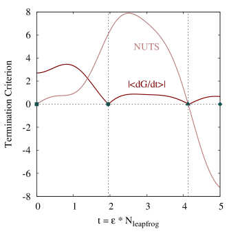
When the correlations are relaxed to $\rho=0.7$, however, the No-U-Turn criterion no longer suffers from premature termination and provides integration times that are far more optimal than those given by the exhaustive termination criterion (Figure 17).

Figure 16: (a) Strong correlations in a two-dimensional Gaussian target distribution, (b) cause the No-U-Turn criterion to terminate (circle) long before the exhaustive criterion for any $\delta$ (triangle). Similarly, (c) the temporal expectations of the effective kinetic energy and effective potential energy vanish after only an incredibly short integration time, making them poor criteria for identifying optimal integration times.

Figure 17: When targeting a two-dimensional Gaussian distribution with weaker correlations the No-U-Turn criterion terminates (triangle) after traversing the level set once, and long after the exhaustion for any exhaustion threshold, $\delta$, (circle), ultimately yielding more effective exploration.

4.2 Performance Experiments

More quantitative evaluations of the termination criteria require comparing the resulting Hamiltonian Markov chains. Both the No-U-Turn Sampler (NUTS) and Exhaustive Hamiltonian Monte Carlo (XHMC) were implemented using a second-order symplectic leapfrog integrator with multiplicative trajectory expansion. NUTS is implemented with a slice sampler over the final trajectory while XHMC utilizes multinomial sampling. Following the original implementation of the No-U-Turn Sampler, I also added an integrator error cutoff which rejects any trajectory $\mathfrak{t}$ sampled around the initial state, $z_{0}$, satisfying

$$H\!\left(z_{0}\right)-H\!\left(z\right)>1000,\,\forall z\in\mathfrak{t}.$$

Without any guidance on how to tune the exhaustion threshold, $\delta$, in all experiments XHMC is run with two nominal thresholds, $\delta=0.1$ and $\delta=0.01$.

All implementations were implemented in Stan (Stan Development Team, 2015a) and run with CmdStan (Stan Development Team, 2015b) using the exhaustions branch (commit: c04d34ee77d831a2817cf3c7671aebc50a3bf825).

Here I consider the performance of both samplers on an identically and independently distributed Gaussian target, a correlated Gaussian target, and a more realistic item response theory model.

4.2.1 IID Gaussian Target

The $100$-dimensional IID Gaussian target with $\rho=0$ is particularly nice because the optimal implementation can be identified analytically. For example, the marginal energy distribution is $\chi^{2}$ with $100$ degrees of freedom while the variation in the momentum resampling is given by a $\chi^{2}$ with $50$ degrees of freedom, sufficiently wide to ensure rapid mixing between the level sets (Figure 18a).

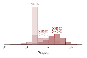
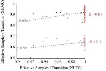
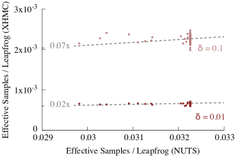
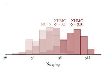
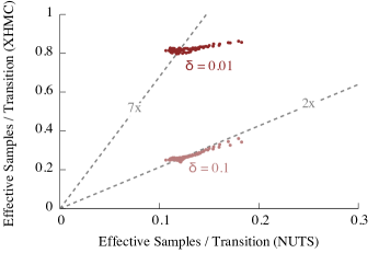
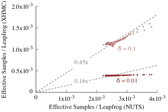
Similarly, because every trajectory oscillates with the period $2\pi$ independent of the level set or the initial point, the optimal maximal integration time is given by $T(z)=2\pi$ with the corresponding optimal trajectory length given by $L=2\pi/\epsilon\sim 64$ leapfrog steps. NUTS integrates to half of this time, but XHMC tends to integrate for much longer (Figure 18b), resulting in worse effective samples per transition (Figure 18c) and even worse effective samples per leapfrog step (Figure 18d).

The redundant exploration in XHMC is a result of the non-stationarity of the exhaustive termination criterion. For IID targets the time rate of the chance of the virial decomposes into a contribution from each dimension,

$$\frac{\mathrm{d}G}{\mathrm{d}t}=2\sum_{n=1}^{N}(T_{n}-V_{n}),$$

which oscillate to zero at different times depending on the initial state. These contributions add incoherently and the exhaustive termination criterion isn’t satisfied until after each dimension has oscillated through a full period, biasing the final samples towards the initial state and actually increasing the autocorrelations. NUTS, on the other hand, is approximately stationary here and is able to identify near optimal integration times.

Figure 18: (a) A Euclidean-Gaussian disintegration is well-suited to an IID Gaussian target distribution, but the ultimate sampling efficiency is sensitive to the choice of integration time. (b) Both XHMC tunes identify integration times that are too long, resulting in (c) larger autocorrelations and (d) substantially worse computational performance.

4.2.2 Correlated Gaussian Target

Now consider correlating the independent Gaussian components with the covariance

$$\Sigma^{ij}=\rho^{\left|i-j\right|},\rho=0.95.$$

In this case the trajectories are no longer periodic but they are dynamically ergodic, and the rate of convergence to the microcanonical distribution is uniform across all level sets. To see the various phases of convergence I sampled uniformly from static trajectories of varying lengths as described in Section 2.1. Up to lengths of around $2^{7}=128$ leapfrog steps the trajectories converge superlinearly, but afterwards the convergence slows to the expected $\sqrt{t}$ asymptotic rate (Figure 19). Per intuition, optimal performance is achieved when trajectories do not grow into the asymptotic regime.

Figure 19: Two phases of convergence are evident in the autocorrelations of a Hamiltonian Markov chain targeting a correlation Gaussian target distribution. For trajectory lengths below approximately $2^{7}=128$ leapfrog steps the effective sample sizes grows superlinearly, but past that initial window the effective sample sizes grow only with the square root of the number of leapfrog steps. Compare to Figure 5.

In another strong showing, NUTS is able to identify the optimal integration times quite well, while XHMC with the nominal tunes selects integration times that fall into the inefficient asymptotic regime (Figure 20). These longer integration times yield smaller autocorrelations and larger effective sample sizes, but the increases are sublinear and hence computationally inefficient (Table 1). A more careful choice of the exhaustion threshold $\delta$ should lead to better performance, but without any guidance in selecting an optimal value it remains a challenging tuning problem.

Figure 20: As in the IID case NUTS outperforms both naive tunes of XHMC when targeting a correlated Gaussian distribution. (a) Once again the Euclidean-Gaussian disintegration is well-suited and (b) both XHMC tunes identify long integration times. In this case the longer integration times lead to (c) smaller autocorrelations and larger effective sample sizes, but (d) the increase in the effective sample size is not enough to warrant the increase computation.

XHMC	Increase in Total	Increase in Median
Tune	Leapfrog Steps	Effective Sample Size
0.1	$\approx 5$x	$\approx 2\mathrm{x}\approx\sqrt{5}\mathrm{x}$
0.01	$\approx 43$x	$\approx 7\mathrm{x}\approx\sqrt{43}\mathrm{x}$

Table 1: When targeting a correlated Gaussian distribution, the nominal XHMC tunes select long integration times that fall into the asymptotic window where the effective sample size grows only with the square root of the number of steps as expected. These diminishing returns ultimately compromise the performance of the XHMC tunes compared to NUTS. Larger exhaustion thresholds tuned to this target distribution should yield better performance, but identifying the optimal tuning is nontrivial.

4.2.3 Nonlinear Target

Finally let’s consider a target distribution more characteristic of applied problems: 1-PL item response theory model for 50 students,

$$y_{i} \sim\mathrm{Bernoulli}\!\left(\mathrm{logistic}\left(\theta-b_{i}\right)\right)$$

$$b_{i} \sim\mathcal{N}\!\left(0,10\right)$$

$$\theta \sim\mathcal{N}\!\left(0,10\right),$$

where the normal distributions here are specified with a mean and standard deviation. Because the data constrain only the sum of the $\theta$ and the individual $b_{i}$, the likelihood is non-identified, and, although the weakly-informative priors offer some regularization, the posterior suffers from strong nonlinear correlations. Because of these nonlinearities, uniform level set exploration also requires dynamic integration times, providing a significant challenge to the termination criteria.

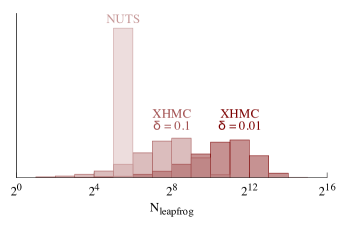
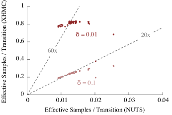
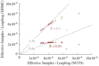
Not surprisingly, the nonlinear correlations cause the No-U-Turn Sampler to terminate prematurely (Figure 21b), resulting in much smaller effective sample sizes relative to the nominal XHMC tunes (Figure 21c) and correspondingly lower computationally efficiency (Figure 21d). The superior performance of XHMC is ultimately due to the fact that the nominal tunes identify integration times that are long without reaching the asymptotic regime (Table 2), which is more coincidental than deliberate.

Figure 21: When targeting the highly-correlated posterior distribution of a 1-PL item response theory model (b) XHMC integrates for much longer than NUTS, (c) yielding much larger effective sample sizes for each parameter and (d) correspondingly higher computational performance.

XHMC	Increase in Total	Increase in Median
Tune	Leapfrog Steps	Effective Sample Size
0.1	$\approx 13$x	$\approx 20\mathrm{x}>13\mathrm{x}$
0.01	$\approx 110$x	$\approx 60\mathrm{x}<110\mathrm{x}$

Table 2: The nominal XHMC tunes not only identify longer integration times than NUTS when targeting the 1-PL posterior, the identified integration times largely avoid the asymptotic regime. In particular, $\delta=0.1$ yields superlinear exploration and improved performance. When the threshold is reduced to $\delta=0.01$, however, the improvement becomes sublinear indicating that the increased integration times are beginning to become asymptotic and yield only diminishing returns.

5 Conclusions and Future Work

Careful analysis of its rich geometric foundations demonstrates that Hamiltonian flow efficiently explores a given target distribution, and admits high-performance Markov Chain Monte Carlo estimation, when the flow is integrated long enough to avoid diffusive behavior but not so long to waste computational resources. This analysis not only provides a theoretical framework for identifying optimal integration times, it also presents new motivation for the No-U-Turn Sampler and inspires the complementary Exhaustive Hamiltonian Monte Carlo algorithm.

The mixed performance of the two algorithms shows that neither criteria is able to robustly identify optimal integration times in all cases and suggests that better termination criteria can still be developed. In particular, the intriguing associations between the No-U-Turn criterion and Poincaré recurrence times intimates that a more explicit application of recurrence may be critical to constructing better criteria.

One substantial benefit of exhaustive termination criterion over the No-U-Turn criterion, however, is the stronger theoretical foundation which makes Exhaustive Hamiltonian Monte Carlo ripe for rigorous formal analysis. This includes, for example, an update of the step size optimality criterion of static Hamiltonian Monte Carlo (Betancourt, Byrne and Girolami, 2014) and a thorough analysis of the statistical ergodicity properties of the algorithm. In particular, the uniform exploration induced by the exhaustive termination criterion has the potential to substantially expand the scope of target distributions to which the implementation is geometrically ergodic.

Finally, we have not yet fully exploited the geometry of the microcanonical disintegration. As noted in Section 1.2, for example, thorough analysis of the marginal autocorrelation on the energy levels can be used to identify poorly chosen cotangent disintegrations and, ideally, motivate optimal ones. Additionally, the natural ergodicity of the Hamiltonian trajectories on their orbits suggest that we should sample not a single point but rather average over the entire trajectory. This averaging gives a Rao-Blackwellization of the microcanonical expectations with the potential to reduce the variance of the overall Markov Chain Monte Carlo estimators, yielding more precise estimators with little added computational burden.

6 Acknowledgements

I warmly thank Bob Carpenter, Andrew Gelman, Daniel Lee, and Dan Simpson for helpful comments on the paper and Sam Livingstone and Simon Byrne for invaluable discussion of the theory and implementation. This work is supported under EPSRC grant EP/J016934/1 and a 2014 EPRSC NCSML Award for PDRA Collaboration.

References

- Betancourt (2013) {barticle}[author] \bauthor\bsnmBetancourt, \bfnmMichael\binitsM. (\byear2013). \btitleGeneralizing the No-U-Turn Sampler to Riemannian Manifolds. \bjournalArXiv e-prints \bvolume1304.1920. \endbibitem
- Betancourt, Byrne and Girolami (2014) {barticle}[author] \bauthor\bsnmBetancourt, \bfnmMichael\binitsM., \bauthor\bsnmByrne, \bfnmSimon\binitsS. and \bauthor\bsnmGirolami, \bfnmMark\binitsM. (\byear2014). \btitleOptimizing The Integrator Step Size for Hamiltonian Monte Carlo. \bjournalArXiv e-prints \bvolume1410.5110. \endbibitem
- Betancourt et al. (2014) {barticle}[author] \bauthor\bsnmBetancourt, \bfnmMichael\binitsM., \bauthor\bsnmByrne, \bfnmSimon\binitsS., \bauthor\bsnmLivingstone, \bfnmSamuel\binitsS. and \bauthor\bsnmGirolami, \bfnmMark\binitsM. (\byear2014). \btitleThe Geometric Foundations of Hamiltonian Monte Carlo. \bjournalArXiv e-prints \bvolume1410.5110. \endbibitem
- Brooks et al. (2011) {bbook}[author] \beditor\bsnmBrooks, \bfnmSteve\binitsS., \beditor\bsnmGelman, \bfnmAndrew\binitsA., \beditor\bsnmJones, \bfnmGalin L.\binitsG. L. and \beditor\bsnmMeng, \bfnmXiao-Li\binitsX.-L., eds. (\byear2011). \btitleHandbook of Markov Chain Monte Carlo. \bpublisherCRC Press, \baddressNew York. \endbibitem
- Campos and Sanz-Serna (2015) {barticle}[author] \bauthor\bsnmCampos, \bfnmCédric M\binitsC. M. and \bauthor\bsnmSanz-Serna, \bfnmJM\binitsJ. (\byear2015). \btitleExtra Chance Generalized Hybrid Monte Carlo. \bjournalJournal of Computational Physics \bvolume281 \bpages365–374. \endbibitem
- Cancès et al. (2005) {barticle}[author] \bauthor\bsnmCancès, \bfnmEric\binitsE., \bauthor\bsnmCastella, \bfnmFrançois\binitsF., \bauthor\bsnmChartier, \bfnmPhilippe\binitsP., \bauthor\bsnmFaou, \bfnmErwan\binitsE., \bauthor\bsnmBris, \bfnmClaude Le\binitsC. L., \bauthor\bsnmLegoll, \bfnmFrédéric\binitsF. and \bauthor\bsnmTurinici, \bfnmGabriel\binitsG. (\byear2005). \btitleLong-Time Averaging for Integrable Hamiltonian Dynamics. \bjournalNumer. Math. \bvolume100 \bpages211–232. \endbibitem
- Diaconis and Freedman (1999) {barticle}[author] \bauthor\bsnmDiaconis, \bfnmPersi\binitsP. and \bauthor\bsnmFreedman, \bfnmDavid\binitsD. (\byear1999). \btitleIterated Random Functions. \bjournalSIAM review \bvolume41 \bpages45–76. \endbibitem
- Duane et al. (1987) {barticle}[author] \bauthor\bsnmDuane, \bfnmSimon\binitsS., \bauthor\bsnmKennedy, \bfnmA. D.\binitsA. D., \bauthor\bsnmPendleton, \bfnmBrian J.\binitsB. J. and \bauthor\bsnmRoweth, \bfnmDuncan\binitsD. (\byear1987). \btitleHybrid Monte Carlo. \bjournalPhysics Letters B \bvolume195 \bpages216 - 222. \endbibitem
- Hairer, Lubich and Wanner (2006) {bbook}[author] \bauthor\bsnmHairer, \bfnmE.\binitsE., \bauthor\bsnmLubich, \bfnmC.\binitsC. and \bauthor\bsnmWanner, \bfnmG.\binitsG. (\byear2006). \btitleGeometric Numerical Integration: Structure-Preserving Algorithms for Ordinary Differential Equations. \bpublisherSpringer, \baddressNew York. \endbibitem
- Hofer and Zehnder (2011) {bbook}[author] \bauthor\bsnmHofer, \bfnmHelmut\binitsH. and \bauthor\bsnmZehnder, \bfnmEduard\binitsE. (\byear2011). \btitleSymplectic Invariants and Hamiltonian Dynamics. \bseriesModern Birkhäuser Classics. \bpublisherBirkhäuser Verlag, Basel. \endbibitem
- Hoffman and Gelman (2014) {barticle}[author] \bauthor\bsnmHoffman, \bfnmMatthew D.\binitsM. D. and \bauthor\bsnmGelman, \bfnmAndrew\binitsA. (\byear2014). \btitleThe No-U-Turn Sampler: Adaptively Setting Path Lengths in Hamiltonian Monte Carlo. \bjournalJournal of Machine Learning Research \bvolume15 \bpages1593–1623. \endbibitem
- Horowitz (1991) {barticle}[author] \bauthor\bsnmHorowitz, \bfnmAlan M\binitsA. M. (\byear1991). \btitleA Generalized Guided Monte Carlo Algorithm. \bjournalPhysics Letters B \bvolume268 \bpages247–252. \endbibitem
- José and Saletan (1998) {bbook}[author] \bauthor\bsnmJosé, \bfnmJorge V.\binitsJ. V. and \bauthor\bsnmSaletan, \bfnmEugene J.\binitsE. J. (\byear1998). \btitleClassical Dynamics: A Contemporary Approach. \bpublisherCambridge University Press, \baddressNew York. \endbibitem
- Lee (2011) {bbook}[author] \bauthor\bsnmLee, \bfnmJohn M\binitsJ. M. (\byear2011). \btitleIntroduction to Topological Manifolds. \bpublisherSpringer. \endbibitem
- Leimkuhler and Reich (2004) {bbook}[author] \bauthor\bsnmLeimkuhler, \bfnmB.\binitsB. and \bauthor\bsnmReich, \bfnmS.\binitsS. (\byear2004). \btitleSimulating Hamiltonian Dynamics. \bpublisherCambridge University Press, \baddressNew York. \endbibitem
- McLachlan, Perlmutter and Quispel (2004) {barticle}[author] \bauthor\bsnmMcLachlan, \bfnmRobert I\binitsR. I., \bauthor\bsnmPerlmutter, \bfnmMatthew\binitsM. and \bauthor\bsnmQuispel, \bfnmGRW\binitsG. (\byear2004). \btitleOn the Nonlinear Stability of Symplectic Integrators. \bjournalBIT Numerical Mathematics \bvolume44 \bpages99–117. \endbibitem
- Neal (1994) {barticle}[author] \bauthor\bsnmNeal, \bfnmRadford M\binitsR. M. (\byear1994). \btitleAn Improved Acceptance Procedure for the Hybrid Monte Carlo Algorithm. \bjournalJournal of Computational Physics \bvolume111 \bpages194–203. \endbibitem
- Neal (2011) {bincollection}[author] \bauthor\bsnmNeal, \bfnmR. M.\binitsR. M. (\byear2011). \btitleMCMC Using Hamiltonian Dynamics. In \bbooktitleHandbook of Markov Chain Monte Carlo (\beditor\bfnmSteve\binitsS. \bsnmBrooks, \beditor\bfnmAndrew\binitsA. \bsnmGelman, \beditor\bfnmGalin L.\binitsG. L. \bsnmJones and \beditor\bfnmXiao-Li\binitsX.-L. \bsnmMeng, eds.) \bpublisherCRC Press, \baddressNew York. \endbibitem
- Petersen (1989) {bbook}[author] \bauthor\bsnmPetersen, \bfnmKarl\binitsK. (\byear1989). \btitleErgodic Theory. \bpublisherCambridge University Press. \endbibitem
- Quas (1991) {barticle}[author] \bauthor\bsnmQuas, \bfnmAnthony N.\binitsA. N. (\byear1991). \btitleOn Representations of Markov Chains by Random Smooth Maps. \bjournalBull. London Math. Soc. \bvolume23 \bpages487–492. \endbibitem
- Robert and Casella (1999) {bbook}[author] \bauthor\bsnmRobert, \bfnmChristian P\binitsC. P. and \bauthor\bsnmCasella, \bfnmGeorge\binitsG. (\byear1999). \btitleMonte Carlo Statistical Methods. \bpublisherSpringer New York. \endbibitem
- Sohl-Dickstein, Mudigonda and DeWeese (2014) {binproceedings}[author] \bauthor\bsnmSohl-Dickstein, \bfnmJascha\binitsJ., \bauthor\bsnmMudigonda, \bfnmMayur\binitsM. and \bauthor\bsnmDeWeese, \bfnmMichael\binitsM. (\byear2014). \btitleHamiltonian Monte Carlo Without Detailed Balance. In \bbooktitleProceedings of the 31st International Conference on Machine Learning \bpages719–726. \endbibitem
- Stan Development Team (2015a) {bmisc}[author] \bauthor\bsnmStan Development Team (\byear2015a). \btitleStan: A C++ Library for Probability and Sampling, Version 2.8.0. \bhowpublishedhttp://mc-stan.org/. \endbibitem
- Stan Development Team (2015b) {bmisc}[author] \bauthor\bsnmStan Development Team (\byear2015b). \btitleCmdStan: The command-line interface to Stan, Version 2.8.0. \bhowpublishedhttp://mc-stan.org/cmdstan.html. \endbibitem
- Tierney (1998) {barticle}[author] \bauthor\bsnmTierney, \bfnmLuke\binitsL. (\byear1998). \btitleA Note on Metropolis-Hastings Kernels for General State Spaces. \bjournalThe Annals of Applied Probability \bvolume8 \bpages1–9. \endbibitem
- Zaslavsky (2008) {bbook}[author] \bauthor\bsnmZaslavsky, \bfnmGeorge M.\binitsG. M. (\byear2008). \btitleHamiltonian Chaos and Fractional Dynamics. \bpublisherOxford University Press, Oxford. \endbibitem