Analysis of a Stochastic Switching Model of Freeway Traffic Incidents

Li Jin and Saurabh Amin L. Jin and S. Amin are with the Department of Civil and Environmental Engineering, Massachusetts Institute of Technology, Cambridge, MA 02139 USA (e-mails: jnl@mit.edu; amins@mit.edu)
Abstract

This article introduces a model for freeway traffic dynamics under stochastic capacity-reducing incidents, and provides insights for freeway incident management by analyzing long-time (stability) properties of the proposed model. Incidents on a multi-cell freeway are modeled by reduction in capacity at the affected freeway sections, which occur and clear according to a Markov chain. We develop conditions under which the traffic queue induced by stochastic incidents is bounded. A necessary condition is that the demand must not exceed the time-average capacity adjusted for spillback. A sufficient condition, in the form of a set of bilinear inequalities, is also established by constructing a Lyapunov function and applying the classical Foster-Lyapunov drift condition. Both conditions can be easily verified for realistic instances of the stochastic incident model. Our analysis relies on the construction of a globally attracting invariant set, and exploits the properties of the traffic flow dynamics. We use our results to analyze the impact of stochastic capacity fluctuation (frequency, intensity, and spatial correlation) on the throughput of a freeway segment.

Index terms: Traffic control, Stability analysis, Piecewise-deterministic Markov processes.

1 Introduction

Freeway traffic networks are prone to capacity disruptions, for example, crashes, road blockage, and other capacity-reducing incidents [21, 38, 24, 28]. In practice, these events can introduce significant congestion in freeways [29, 36]. To design traffic control strategies that reduce the congestion and throughput loss resulting from such disruptions, we need to systematically analyze traffic dynamics under stochastic capacity fluctuations. This article introduces a stochastic switching model of freeway traffic dynamics under capacity fluctuations, and studies its stability (in the sense of bounded traffic queue) under fixed inflows.

According to a recent report by the U.S. Federal Highway Administration [34, pp. 97], the current practice of managing freeway incidents is to consider each scenario on a case-by-case basis: a traffic manager assesses the impact of detected incidents and responds based on past practice or personal judgment. Some examples of actually implemented traffic incident management strategies in this class are reported in [6]. This approach is also considered in recent research on traffic management under capacity disruptions [16, 37, 31, 27]. However, in practice, the implementation of scenario-specific strategies cannot be readily assigned a performance guarantee. Moreover, the scenario-based approach does not provide guidelines on designing control strategies that are robust to disruptions not captured by the assumed set of scenarios. Thus, a model-based approach for traffic control under disruptions is desirable. In this article, we follow the model-based approach and study the stability of the well-known cell-transmission model (CTM, see [10, 15]) of freeways under stochastic capacity disruptions. Our stochastic capacity model captures the main features of capacity-reducing incidents: capacity drop, frequency, and duration. We combine this model with the CTM and obtain a stochastic switching CTM (i.e. SS-CTM) that can be used to study the throughput and delay in incident-prone freeways.

Before introducing our model and results, we briefly summarize earlier work on stochastic extensions of CTM. Sumalee et al. [39] proposed a CTM with parameters subject to random noise; however, their model is largely motivated by the intrinsic randomness in the demand and the flow-density relation, but does not explicitly model capacity-reducing events. Zhong et al. [41] consider a closely related model in which traffic flow dynamics randomly switch between free-flow and congested modes. The authors of [41] study an optimal control problem over a finite time horizon. In contrast, our model admits a richer class of stochastic disruptions. We focus on the long-time properties of the traffic queue resulting from stochastic disruptions. Indeed, stability of traffic queue is critical for steady-state performance guarantee in any stochastic optimal control of freeway systems, such as that studied in [41]. Our model is also related to the stochastic models used in [23, 33] in the context of traffic incident management. However, these models do not capture the dynamic propagation of incident-induced congestion (spillback), which is a critical mechanism affecting the traffic dynamics in freeways.

In our SS-CTM (formally defined in Section 2), the capacity of a freeway section switches between a finite set of values (modes); the switches are governed by a continuous-time finite-state Markov chain. The mode transitions can represent abrupt changes in traffic dynamics including: (i) occurrence of primary incidents [21, 1], (ii) occurrence of secondary incidents [23, 35], and (iii) clearance of incidents [38, 18]. In a given mode, the traffic density in each section (the continuous state of the model) evolves according to the CTM. The mode transitions essentially govern the build-up and release of traffic queues in the system.

We note that actual capacity fluctuation may be more complicated than the finite-state Markov model [20, 17]. However, this model is adequate to study the build-up and release of traffic queues due to stochastic capacity, and also enables a tractable analysis of long-time properties of the traffic queues. In a related work [20], we showed that calibration of this model is simple, and that it satisfactorily captures the stochastic variation of capacity in practical situations; see [41, 22, 2] for related models.

The SS-CTM can be viewed as a piecewise-deterministic Markov process (PDMP) without random resets of the continuous state [12, 3]. Since the transition rates are time-invariant, this model is also a specific example of Markovian jump systems [5, 40]. In our previous work [18], we provided a preliminary analysis of the accessible set of the model. In this article, we present a rather complete framework for analyzing the stability of the SS-CTM, based on long-time properties of the deterministic mode dynamics and the Markovian mode transition process.

Our analysis is motivated by the following practical question: on an incident-prone freeway, under what conditions does the long-time average of the total number of vehicles on the freeway (including the upstream queue) remain bounded? We are interested in deriving intuitive and verifiable stability criteria for the SS-CTM. Specifically, we consider boundedness of the moment generating function (MGF) of the total number of vehicles on the freeway in our analysis. In fact, since the traffic density in each cell is upper-bounded by the jam density, boundedness of the total number of vehicles is in line with the boundedness of the upstream queue. Our notion of stability is similar to that considered by Dai and Meyn [11], who considered boundedness of the moments of the queue lengths.

The main results of this article (Theorems 1 and 2; presented in Section 3) include a necessary condition and a sufficient condition for stability of the SS-CTM with fixed inflows111Our setup can be extended to model time-varying or controlled inflows; however, this extension is not within the scope of this article. and an ergodic mode transition process. To establish these results, we build on the theory of stability of continuous-time Markov processes [3, 32, 14]. Note, however, that the application of standard stability results to our setting is not straightforward due to non-linearity of the CTM dynamics. In this article, we exploit the properties of the mode transition process and the CTM dynamics to develop a tractable approach to characterizing the set of stabilizing inflow vectors – specifically, an over- and an under-approximation of this set. We now introduce the main features of our stability conditions.

Theorem 1 is a necessary condition for stability; it states that the SS-CTM is stable only if for each freeway section (cell), the traffic flow does not exceed the time-average of the “spillback-adjusted” capacity. The notion of spillback-adjusted capacity essentially captures the effect of downstream congestion (i.e. spillback) resulting from capacity fluctuations on the traffic discharging ability of each cell. To the best of our knowledge, this notion has not been reported previously in the literature. The computation of spillback-adjusted capacity builds on the construction of an invariant set that is also globally attracting (Proposition 1). Using this construction, we obtain that the capacity fluctuation can result in an unbounded traffic queue even when the inflow in each cell is less than the average capacity; this property essentially results from the effect of traffic spillback. Theorem 1 also provides a way to identify an over-approximation of the set of stabilizing inflow vectors (i.e. the inflows that satisfy the necessary condition).

To establish the sufficient condition for stability (Theorem 2), we consider a well-known approach formalized by Meyn and Tweedie [32]. Application of this approach to our model is challenging, since it requires verification of the Foster-Lyapunov drift condition, i.e. a set of non-linear inequalities, everywhere over the invariant set (which we construct in Proposition 1). To resolve this issue, we construct a switched, exponential Lyapunov function that assigns appropriate weights to the traffic densities in various cells, depending on the cells’ locations and inflow-capacity ratios. We also utilize properties of the CTM dynamics to show that the drift condition holds everywhere over the invariant set if a finite set of bilinear inequalities is feasible. Consequently, standard computational tools [30] can be used to check whether a given inflow vector maintains stability of SS-CTM or not.

Overall, these results enable a systematic analysis of the congestion induced by stochastic incidents. In Section 4, we provide examples to show how Theorems 1 and 2 can be used to characterize the set of stabilizing inflow vectors. We also comment on the tightness of our results, i.e., the gap between the necessary and the sufficient condition. In addition, we present illustrative examples to study the impact of capacity fluctuation (including its frequency, intensity, and spatial correlation) on the throughput of a freeway section.

Finally, all technical proofs are presented in Appendix.

2 Stochastic Switching Cell Transmission Model

In this section, we define the stochastic switching cell transmission model (SS-CTM). To develop this model, we introduce a Markovian capacity model, and combine it with the classical CTM [10]. We also introduce key definitions that are needed for our subsequent analysis.

2.1 Markovian capacity model

Consider a freeway consisting of K𝐾K cells, as shown in Figure 1. The capacity (or saturation rate, in vehicles per hour, or veh/hr) of the k𝑘k-th cell at time t0𝑡0t\geq 0 is denoted by Fk(t)subscript𝐹𝑘𝑡{F}_{k}(t). Let F(t)=[F1(t),,FK(t)]T𝐹𝑡superscriptsubscript𝐹1𝑡subscript𝐹𝐾𝑡𝑇{F}(t)=[{F}_{1}(t),\ldots,{F}_{K}(t)]^{T} denote the vector of cell capacities at time t𝑡t. One can interpret Fk(t)subscript𝐹𝑘𝑡{F}_{k}(t) as the maximum rate at which cell k𝑘k can discharge traffic to the downstream cell at time t𝑡t.

Refer to caption
Figure 1: SS-CTM with K𝐾K cells. Cell 1 includes an infinite-sized buffer to accommodate the upstream queue.

To model stochastic capacity disruptions, we assume that F(t)𝐹𝑡{F}(t) is a finite-state Markov process. Specifically, let \mathcal{I} be a finite set of modes of the freeway and let m=||𝑚m=|\mathcal{I}|. Each mode i𝑖i\in\mathcal{I} is associated with a vector of cell capacities Fi=[F1i,,FKi]Tsuperscript𝐹𝑖superscriptsuperscriptsubscript𝐹1𝑖superscriptsubscript𝐹𝐾𝑖𝑇{F}^{i}=[{F}_{1}^{i},\ldots,{F}_{K}^{i}]^{T}. We define

Fkmin=miniFki,Fkmax=maxiFki,formulae-sequencesuperscriptsubscript𝐹𝑘subscript𝑖superscriptsubscript𝐹𝑘𝑖superscriptsubscript𝐹𝑘subscript𝑖superscriptsubscript𝐹𝑘𝑖\displaystyle{F}_{k}^{\min}=\min_{i\in\mathcal{I}}{F}_{k}^{i},\quad{F}_{k}^{\max}=\max_{i\in\mathcal{I}}{F}_{k}^{i}, (1a)

and refer to Fkmaxsuperscriptsubscript𝐹𝑘{F}_{k}^{\max} as the normal (maximum) capacity of cell k𝑘k. For ease of presentation, we assume an identical normal capacity for all cells throughout the article, i.e. Fkmax=Fmaxsuperscriptsubscript𝐹𝑘superscript𝐹F_{k}^{\max}=F^{\max} for k=1,2,,K𝑘12𝐾k=1,2,\ldots,K.

In our model, a mode represents a particular configuration of capacities at various locations (cells). We say that the freeway is in the normal mode if the maximum capacity is available at every cell. We model an incident in cell k𝑘k by introducing a mode i𝑖i such that Fki<Fmaxsuperscriptsubscript𝐹𝑘𝑖superscript𝐹{F}_{k}^{i}<{F}^{\max} and Fhi=Fmaxsuperscriptsubscript𝐹𝑖superscript𝐹{F}_{h}^{i}={F}^{\max} for hk𝑘h\neq k. Transition from the normal mode to mode i𝑖i can be viewed as occurrence of an incident in cell k𝑘k; similarly, the transition from i𝑖i to the normal mode can be viewed as clearance of the incident. Furthermore, we call the k𝑘k-th cell an incident hotspot if Fkmin<Fmaxsuperscriptsubscript𝐹𝑘superscript𝐹F_{k}^{\min}<F^{\max}.

Note that the Markovian capacity model can be used to represent more complex situations. For example, two modes can be associated with incidents in the same cell(s), but with different values of capacities, reflecting the difference in incident intensities (e.g. minor and major). Furthermore, the occurrence of secondary (or induced) incidents [23] can be modeled as a transition from a mode with an incident in a single cell to a mode with incidents in multiple cells.

Throughout this article, we use i𝑖i to denote elements of \mathcal{I}, and use I(t)𝐼𝑡I(t) to denote the stochastic mode of the freeway at time t𝑡t. The mode I(t)𝐼𝑡I(t) switches according to a continuous-time, finite-state Markov chain defined over the set \mathcal{I} with (time-invariant) transition rates {λij;i,j}subscript𝜆𝑖𝑗𝑖𝑗\{\lambda_{ij};i,j\in\mathcal{I}\}. We assume that λii=0subscript𝜆𝑖𝑖0\lambda_{ii}=0 for each i𝑖i\in\mathcal{I}; note that this is without loss of generality, as inclusion of self-transitions would not affect the traffic flow dynamics. Let νi=jλijsubscript𝜈𝑖subscript𝑗subscript𝜆𝑖𝑗\nu_{i}=\sum_{j\in\mathcal{I}}\lambda_{ij} and define the transition matrix as follows:

Λ=[ν1λ12λ1mλ21ν2λ2mλm1λm2νm].Λdelimited-[]subscript𝜈1subscript𝜆12subscript𝜆1𝑚subscript𝜆21subscript𝜈2subscript𝜆2𝑚subscript𝜆𝑚1subscript𝜆𝑚2subscript𝜈𝑚\displaystyle\Lambda=\left[\begin{array}[]{llll}-\nu_{1}&\lambda_{12}&\ldots&\lambda_{1m}\\ \lambda_{21}&-\nu_{2}&\ldots&\lambda_{2m}\\ \vdots&\vdots&\ddots&\vdots\\ \lambda_{m1}&\lambda_{m2}&\ldots&-\nu_{m}\\ \end{array}\right]. (6)

We assume the following for the mode switching process:

Assumption 1.

The finite-state Markov process {I(t);t0}𝐼𝑡𝑡0\{I(t);t\geq 0\} is ergodic.

This assumption ensures that the dwell times in each mode are finite almost surely (a.s.). Under this assumption, the process {I(t);t0}𝐼𝑡𝑡0\{I(t);t\geq 0\} admits a unique steady-state probability distribution 𝗉=[𝗉1,,𝗉m]𝗉subscript𝗉1subscript𝗉𝑚\mathsf{p}=[\mathsf{p}_{1},\ldots,\mathsf{p}_{m}] satisfying:

𝗉Λ=0,|𝗉|=1,𝗉0,formulae-sequence𝗉Λ0formulae-sequence𝗉1𝗉0\displaystyle\mathsf{p}\Lambda=0,\;|\mathsf{p}|=1,\;\mathsf{p}\geq 0, (7)

where |||\cdot| indicates the 1-norm of (row or column) vectors [14].

2.2 Traffic flow under stochastic capacities

The formal definition of the SS-CTM is as follows:

Definition 1.

The SS-CTM is a tuple ,𝒩,,Λ,G𝒩Λ𝐺\langle\mathcal{I},\mathcal{N},\mathcal{R},\Lambda,G\rangle, where

  • -

    \mathcal{I} is a finite set of modes (discrete state space) with ||=m𝑚|\mathcal{I}|=m,

  • -

    𝒩=[0,)×[0,nmax]K1𝒩0superscript0superscript𝑛𝐾1\mathcal{N}=[0,\infty)\times[0,{n}^{\max}]^{K-1} is the set of traffic densities (continuous state space),

  • -

    0Ksuperscriptsubscriptabsent0𝐾absent\mathcal{R}\subseteq_{\geq 0}^{K} is the set of inflow vectors,

  • -

    Λm×msuperscript𝑚𝑚Λabsent\Lambda\in^{m\times m} is the transition rate matrix governing the mode transitions, and

  • -

    G:×𝒩×K:𝐺superscript𝐾𝒩absentG:\mathcal{I}\times\mathcal{N}\times\mathcal{R}\to^{K} is the vector field governing the continuous dynamics.

We have defined \mathcal{I} and ΛΛ\Lambda, and now introduce 𝒩𝒩\mathcal{N}, \mathcal{R}, and G𝐺G.

Let Nk(t)subscript𝑁𝑘𝑡{N}_{k}(t) denote the traffic density (in vehicles per mile, veh/mi) in the k𝑘k-th cell at time t𝑡t, as shown in Figure 1. Traffic density Nk(t)subscript𝑁𝑘𝑡{N}_{k}(t) is non-negative and upper bounded by nkmaxsubscriptsuperscript𝑛𝑘{n}^{\max}_{k}, the k𝑘k-th cell’s jam density. The K𝐾K-dimensional vector N(t)=[N1(t),N2(t),,NK(t)]T𝒩𝑁𝑡superscriptsubscript𝑁1𝑡subscript𝑁2𝑡subscript𝑁𝐾𝑡𝑇𝒩N(t)=\left[{N}_{1}(t),{N}_{2}(t),\dots,{N}_{K}(t)\right]^{T}\in\mathcal{N} represents the stochastic continuous state of the SS-CTM.

For ease of presentation, we assume that each cell has the unit length of 1 mi. Furthermore, each cell has identical parameters, including the free-flow speed v𝑣v, the congestion-wave speed w𝑤w, the jam density nmaxsuperscript𝑛{n}^{\max}, and – as mentioned before – an identical normal capacity Fmaxsuperscript𝐹{F}^{\max}. The unit of v𝑣v and w𝑤w is miles per hour (mi/hr). We define the critical density of vehicles as

ncrit=Fmaxv.superscript𝑛critsuperscript𝐹𝑣\displaystyle n^{\mathrm{crit}}=\frac{{F}^{\max}}{v}. (8)

The sending flows Sksubscript𝑆𝑘S_{k} and the receiving flows Rksubscript𝑅𝑘R_{k} can be written as follows:

Sk(i,nk)=min{vnk,Fki},k=1,2,,K,formulae-sequencesubscript𝑆𝑘𝑖subscript𝑛𝑘𝑣subscript𝑛𝑘superscriptsubscript𝐹𝑘𝑖𝑘12𝐾\displaystyle S_{k}(i,{n}_{k})=\min\left\{v{n}_{k},{F}_{k}^{i}\right\},\;k=1,2,\ldots,K, (9a)
Rk(nk)=w(nmaxnk),k=2,3,,K.formulae-sequencesubscript𝑅𝑘subscript𝑛𝑘𝑤superscript𝑛subscript𝑛𝑘𝑘23𝐾\displaystyle R_{k}({n}_{k})=w({n}^{\max}-{n}_{k}),\;k=2,3,\ldots,K. (9b)

Thus, Sksubscript𝑆𝑘S_{k} is the traffic flow that cell k𝑘k can discharge downstream and Rksubscript𝑅𝑘R_{k} is the traffic flow from upstream that cell k𝑘k can accommodate. The receiving flow of cell 1 will be discussed later in this subsection. Following [10], we assume that,

k{1,2,,K},maxiISk(i,ncrit)Rk(ncrit),formulae-sequencefor-all𝑘12𝐾subscript𝑖𝐼subscript𝑆𝑘𝑖superscript𝑛critsubscript𝑅𝑘superscript𝑛crit\displaystyle\forall k\in\{1,2,\ldots,K\},\;\max_{i\in I}S_{k}(i,n^{\mathrm{crit}})\leq R_{k}(n^{\mathrm{crit}}),

which, along with (8) and (9), implies that,

Fmaxvwv+wnmax.superscript𝐹𝑣𝑤𝑣𝑤superscript𝑛\displaystyle{F}^{\max}\leq\frac{vw}{v+w}{n}^{\max}. (10)

Let r=[r1,r2,,rK]T=0K𝑟superscriptsubscript𝑟1subscript𝑟2subscript𝑟𝐾𝑇superscriptsubscriptabsent0𝐾absentr=\left[r_{1},r_{2},\ldots,r_{K}\right]^{T}\in\mathcal{R}=_{\geq 0}^{K} denote the inflow vector to the freeway; the unit of rksubscript𝑟𝑘r_{k} is veh/hr. Throughout this article, we assume that the freeway is subject to a fixed (i.e. time-invariant) inflow vector. Importantly, we also make the standard assumption that, for each cell k𝑘k, the on-ramp flow rksubscript𝑟𝑘r_{k} is prioritized over the sending inflow Sk1subscript𝑆𝑘1S_{k-1} from the upstream cell [15]. Under this priority rule, the flow (in veh/hr) from cell k𝑘k to cell k+1𝑘1k+1, denoted by fksubscript𝑓𝑘f_{k}, is given by the flow function (i.e., the so-called fundamental diagram):

f0=0,subscript𝑓00\displaystyle f_{0}=0, (11a)
fk(i,nk,nk+1,rk+1)=min{βkSk(i,nk),\displaystyle f_{k}(i,{n}_{k},{n}_{k+1},r_{k+1})=\min\{\beta_{k}S_{k}(i,{n}_{k}),
(Rk+1(nk+1)rk+1)+},k=1,2,,K1,\displaystyle\hskip 28.90755pt(R_{k+1}({n}_{k+1})-r_{k+1})_{+}\},\;k=1,2,\ldots,K-1, (11b)
fK(i,nK)=βKSK(i,nK).subscript𝑓𝐾𝑖subscript𝑛𝐾subscript𝛽𝐾subscript𝑆𝐾𝑖subscript𝑛𝐾\displaystyle f_{K}(i,{n}_{K})=\beta_{K}S_{K}(i,{n}_{K}). (11c)

where ()+subscript(\cdot)_{+} stands for the positive part and βk=fk/(fk+sk)(0,1]subscript𝛽𝑘subscript𝑓𝑘subscript𝑓𝑘subscript𝑠𝑘01\beta_{k}=f_{k}/(f_{k}+s_{k})\in(0,1] denotes the fixed mainline ratio, i.e. the fraction of traffic from cell k𝑘k entering cell k+1𝑘1k+1. The off-ramp flow sksubscript𝑠𝑘s_{k} from cell k𝑘k is given by sk(t)=(1/βk1)fk(t)subscript𝑠𝑘𝑡1subscript𝛽𝑘1subscript𝑓𝑘𝑡s_{k}(t)=(1/\beta_{k}-1)f_{k}(t) for k=1,2,,K𝑘12𝐾k=1,2,\ldots,K.

Let f(i,n,r)𝑓𝑖𝑛𝑟f(i,{n},r) denote the K𝐾K-dimensional vector of flows. For notational convenience, we denote Sk(t)=Sk(I(t),Nk(t))subscript𝑆𝑘𝑡subscript𝑆𝑘𝐼𝑡subscript𝑁𝑘𝑡S_{k}(t)=S_{k}(I(t),{N}_{k}(t)), Rk(t)=Rk(Nk(t))subscript𝑅𝑘𝑡subscript𝑅𝑘subscript𝑁𝑘𝑡R_{k}(t)=R_{k}({N}_{k}(t)), and f(t)=f(I(t),N(t),r)𝑓𝑡𝑓𝐼𝑡𝑁𝑡𝑟f(t)=f(I(t),N(t),r). We say that cell k𝑘k is experiencing spillback at time t𝑡t if βkSk(t)>Rk+1(t)rk+1subscript𝛽𝑘subscript𝑆𝑘𝑡subscript𝑅𝑘1𝑡subscript𝑟𝑘1\beta_{k}S_{k}(t)>R_{k+1}(t)-r_{k+1}, i.e. if the sending flow from cell k𝑘k exceeds the receiving flow of cell k+1𝑘1k+1.

Due to spillback, there might be traffic queues at the entrances (on-ramps) to the freeway. We track the queue upstream to cell 1 by assuming that cell 1 has a buffer with infinite space to admit this queue, i.e. n1max=subscriptsuperscript𝑛1{n}^{\max}_{1}=\infty (see Figure 1). However, we do not consider the on-ramp queues (i.e. queues at on-ramps to cells 2,3,,K23𝐾2,3,\ldots,K). Note that not including the on-ramp queues to cells 2 through K𝐾K does not affect our stability analysis of the upstream queue, since our priority rule implies that the boundedness of the upstream queue is a sufficient condition for the boundedness of the on-ramp queues. Hence, we denote the continuous state space of the SS-CTM as 𝒩=[0,)×[0,nmax]K1𝒩0superscript0superscript𝑛𝐾1\mathcal{N}=[0,\infty)\times[0,{n}^{\max}]^{K-1}.

By mass conservation, traffic density in each cell evolves as follows [15]:

N˙k(t)=fk1(t)+rkfk(t)/βk,k=1,2,,K.formulae-sequencesubscript˙𝑁𝑘𝑡subscript𝑓𝑘1𝑡subscript𝑟𝑘subscript𝑓𝑘𝑡subscript𝛽𝑘𝑘12𝐾\displaystyle\dot{N}_{k}(t)=f_{k-1}(t)+r_{k}-f_{k}(t)/\beta_{k},\;k=1,2,\dots,K. (12)

From (11) and (12), we can define the vector field G:×𝒩×n:𝐺superscript𝑛𝒩absentG:\mathcal{I}\times\mathcal{N}\times\mathcal{R}\to^{n} governing the continuous state of the SS-CTM as follows:

G1(i,n,r)=r1f1(i,n1,n2,r2)/β1,subscript𝐺1𝑖𝑛𝑟subscript𝑟1subscript𝑓1𝑖subscript𝑛1subscript𝑛2subscript𝑟2subscript𝛽1\displaystyle G_{1}(i,{n},r)=r_{1}-f_{1}(i,{n}_{1},{n}_{2},r_{2})/\beta_{1}, (13a)
Gk(i,n,r)=fk1(i,nk1,nk,rk)+rksubscript𝐺𝑘𝑖𝑛𝑟subscript𝑓𝑘1𝑖subscript𝑛𝑘1subscript𝑛𝑘subscript𝑟𝑘subscript𝑟𝑘\displaystyle G_{k}(i,{n},r)=f_{k-1}(i,{n}_{k-1},{n}_{k},r_{k})+r_{k}
fk(i,nk,nk+1,rk+1)/βk,k=2,3,,K1,formulae-sequencesubscript𝑓𝑘𝑖subscript𝑛𝑘subscript𝑛𝑘1subscript𝑟𝑘1subscript𝛽𝑘𝑘23𝐾1\displaystyle\quad-f_{k}(i,{n}_{k},{n}_{k+1},r_{k+1})/\beta_{k},\;k=2,3,\ldots,K-1, (13b)
GK(i,n,r)=fK1(i,nK1,nK,rK)+rkfK(i,nK)/βK.subscript𝐺𝐾𝑖𝑛𝑟subscript𝑓𝐾1𝑖subscript𝑛𝐾1subscript𝑛𝐾subscript𝑟𝐾subscript𝑟𝑘subscript𝑓𝐾𝑖subscript𝑛𝐾subscript𝛽𝐾\displaystyle G_{K}(i,{n},r)=f_{K-1}(i,{n}_{K-1},{n}_{K},r_{K})+r_{k}-f_{K}(i,{n}_{K})/\beta_{K}. (13c)

Note that the vector field G𝐺G is bounded and continuous in n𝑛{n}. In a given mode i𝑖i\in\mathcal{I}, the integral curve starting from n𝒩𝑛𝒩{n}\in\mathcal{N}, denoted by ϕti(n)=[ϕti(n)1,,ϕti(n)K]Tsuperscriptsubscriptitalic-ϕ𝑡𝑖𝑛superscriptsuperscriptsubscriptitalic-ϕ𝑡𝑖subscript𝑛1superscriptsubscriptitalic-ϕ𝑡𝑖subscript𝑛𝐾𝑇\phi_{t}^{i}({n})=[\phi_{t}^{i}({n})_{1},\ldots,\phi_{t}^{i}({n})_{K}]^{T}, can be expressed as follows:

ϕti(n)=n+τ=0tG(i,ϕτi(n),r)𝑑τ.superscriptsubscriptitalic-ϕ𝑡𝑖𝑛𝑛superscriptsubscript𝜏0𝑡𝐺𝑖superscriptsubscriptitalic-ϕ𝜏𝑖𝑛𝑟differential-d𝜏\displaystyle\phi_{t}^{i}({n})={n}+\int_{\tau=0}^{t}G\Big{(}i,\phi_{\tau}^{i}({n}),r\Big{)}d\tau. (14)

The hybrid state of the SS-CTM is (I(t),N(t))𝐼𝑡𝑁𝑡(I(t),N(t)) at time t𝑡t, and the hybrid state space is ×𝒩𝒩\mathcal{I}\times\mathcal{N}. The evolution of the discrete (resp. continuous) state is governed by the finite-state Markov process with transition matrix ΛΛ\Lambda (resp. the vector field G𝐺G). For an initial condition (i,n)×𝒩𝑖𝑛𝒩(i,{n})\in\mathcal{I}\times\mathcal{N}, the stochastic process {(I(t),N(t));t0}𝐼𝑡𝑁𝑡𝑡0\{(I(t),N(t));t\geq 0\} is given by

N(t)=n+τ=0tG(I(τ),N(τ),r)𝑑τ,𝑁𝑡𝑛superscriptsubscript𝜏0𝑡𝐺𝐼𝜏𝑁𝜏𝑟differential-d𝜏\displaystyle N(t)={n}+\int_{\tau=0}^{t}G\Big{(}I(\tau),N(\tau),r\Big{)}d\tau, (15a)
Pr{I(t+δ)=j|I(t)=i}=λijδ+o(δ),ji.formulae-sequencePr𝐼𝑡𝛿conditional𝑗𝐼𝑡𝑖subscript𝜆𝑖𝑗𝛿o𝛿𝑗𝑖\displaystyle\Pr\Big{\{}I(t+\delta)=j|I(t)=i\Big{\}}=\lambda_{ij}\delta+\mathrm{o}(\delta),\;j\neq i. (15b)

2.3 Additional definitions

For an SS-CTM with a given inflow vector r𝑟r\in\mathcal{R}, the total number of vehicles |N(t)|𝑁𝑡|N(t)| at time t𝑡t is given by

|N(t)|=k=1KNk(t).𝑁𝑡superscriptsubscript𝑘1𝐾subscript𝑁𝑘𝑡\displaystyle|N(t)|=\sum_{k=1}^{K}{N}_{k}(t). (16)

We say that the SS-CTM is stable if the moment generating function (MGF) of N(t)𝑁𝑡N(t) is bounded on average; i.e., for some finite constant C𝐶C and for each initial condition (i,n)×𝒩𝑖𝑛𝒩(i,{n})\in\mathcal{I}\times\mathcal{N},

lim supt1tτ=0t𝖤[exp(|N(τ)|)]𝑑τC.subscriptlimit-supremum𝑡1𝑡superscriptsubscript𝜏0𝑡𝖤delimited-[]𝑁𝜏differential-d𝜏𝐶\displaystyle\limsup_{t\to\infty}\frac{1}{t}\int_{\tau=0}^{t}\mathsf{E}[\exp(|N(\tau)|)]d\tau\leq C. (17)

Since a bounded MGF implies a bounded p𝑝p-th moment for all p>0𝑝subscriptabsent0p\in\mathbb{Z}_{>0}, our notion of stability is in line with the notion of bounded moments considered by Dai and Meyn [11]. Recall that, in our model, N2(t),,NK(t)subscript𝑁2𝑡subscript𝑁𝐾𝑡{N}_{2}(t),\ldots,{N}_{K}(t) are always upper-bounded by the jam density nmaxsuperscript𝑛{n}^{\max}; therefore, N(t)𝑁𝑡N(t) is bounded if and only if N1(t)subscript𝑁1𝑡{N}_{1}(t) is bounded.

An alternative notion of stability that is used in the analysis of queueing systems [11, 25, 19] and PDMPs [3, 7] is the convergence of the traffic queue towards a unique invariant probability measure. This notion of stability is equivalent to boundedness of the traffic queue in many simple settings (e.g. for M/M/1𝑀𝑀1M/M/1 queues [14] or fluid queueing systems with stochastic service rates [25, 19]). However, convergence to a unique invariant probability measure does not always guarantee bounded moments of the traffic queue, which is of practical significance for freeway traffic management. Therefore, in this article, we consider boundedness of the upstream queue as the stability notion of interest.

A major issue in analyzing the stability of the SS-CTM is to ensure (17) for all initial conditions (i,n)×𝒩𝑖𝑛𝒩(i,{n})\in\mathcal{I}\times\mathcal{N}. We address this issue by constructing a positive invariant set that is also globally attracting and positively invariant [3], i.e. a set 𝒩~𝒩~𝒩𝒩\widetilde{\mathcal{N}}\subseteq\mathcal{N} such that

(Invariant)(i,n)×𝒩~,t0,ϕti(n)𝒩~;formulae-sequence(Invariant)for-all𝑖𝑛~𝒩formulae-sequencefor-all𝑡0superscriptsubscriptitalic-ϕ𝑡𝑖𝑛~𝒩\displaystyle\mbox{(Invariant)}\quad\forall(i,{n})\in\mathcal{I}\times\widetilde{\mathcal{N}},\;\forall t\geq 0,\;\phi_{t}^{i}({n})\in\widetilde{\mathcal{N}}; (18a)
(Attracting)(i,n)×𝒩,I(0)=i,N(0)=n,formulae-sequence(Attracting)for-all𝑖𝑛𝒩formulae-sequence𝐼0𝑖𝑁0𝑛\displaystyle\mbox{(Attracting)}\quad\forall(i,{n})\in\mathcal{I}\times\mathcal{N},\;I(0)=i,{N}(0)={n},
ϵ>0,T0,tT,minν𝒩~N(t)ν2ϵ.formulae-sequencefor-allitalic-ϵ0formulae-sequence𝑇0formulae-sequencefor-all𝑡𝑇subscript𝜈~𝒩subscriptnorm𝑁𝑡𝜈2italic-ϵ\displaystyle\hskip 21.68121pt\forall\epsilon>0,\;\exists T\geq 0,\;\forall t\geq T,\;\min_{\nu\in\widetilde{\mathcal{N}}}\|N(t)-\nu\|_{2}\leq\epsilon. (18b)

For convenience, we henceforth refer to any set satisfying (18a) and (18b) simply as an invariant set. Construction of an invariant set considerably simplifies the proofs of our main results (Theorems 1 and 2), since, to capture long-time behavior of SS-CTM, we only need to consider initial conditions in 𝒩~~𝒩\widetilde{\mathcal{N}} rather than in 𝒩𝒩\mathcal{N}.

Before proceeding further, we introduce two properties of the SS-CTM. First, the natural filtration tsubscript𝑡{\mathcal{F}}_{t} of the SS-CTM is the σ𝜎\sigma-algebra generated by {(I(s),N(s));st}𝐼𝑠𝑁𝑠𝑠𝑡\{(I(s),N(s));s\leq t\} for all t0𝑡0t\geq 0 [12]. Since the realizations of the continuous state are always continuous in time, and since the transition rates λijsubscript𝜆𝑖𝑗\lambda_{ij} are finite and constant, tsubscript𝑡{\mathcal{F}}_{t} is right continuous with left limits (RCLL, or càdlàg [3]). Second, by [3, Proposition 2.1], thanks to the RCLL property, the infinitesimal generator of the SS-CTM with a fixed inflow r𝑟r\in\mathcal{R} can be written as an operator \mathcal{L} as follows:

g(i,n)𝑔𝑖𝑛\displaystyle\mathcal{L}g(i,{n}) =GT(i,n,r)ng(i,n)+jλij(g(j,n)g(i,n)),absentsuperscript𝐺𝑇𝑖𝑛𝑟subscript𝑛𝑔𝑖𝑛subscript𝑗subscript𝜆𝑖𝑗𝑔𝑗𝑛𝑔𝑖𝑛\displaystyle=G^{T}(i,{n},r)\nabla_{n}g(i,{n})+\sum_{j\in\mathcal{I}}\lambda_{ij}\Big{(}g(j,{n})-g(i,{n})\Big{)},
(i,n)×𝒩,for-all𝑖𝑛𝒩\displaystyle\hskip 122.85876pt\forall(i,{n})\in\mathcal{I}\times\mathcal{N}, (19)

where g:×𝒩:𝑔𝒩absentg:\mathcal{I}\times\mathcal{N}\to is a function smooth in the second argument, and ng(i,n)subscript𝑛𝑔𝑖𝑛\nabla_{n}g(i,{n}) is the gradient of g𝑔g with respect to n𝑛{n}.222We consider ngsubscript𝑛𝑔\nabla_{n}g as a column vector. We utilize the expression of the infinitesimal generator in our stability analysis (while applying the Foster-Lyapunov drift condition [32] in Appendix C).

3 Stability of SS-CTM

In this section, we present our results and demonstrate their application via a simple example. The proofs for these results are available in Appendix.

3.1 Main results

Our results include a necessary condition (Theorem 1) and a sufficient condition (Theorem 2) for the stability of the SS-CTM under fixed inflows. Both of these conditions rely on the construction of a “rectangular” invariant set of the following form:

𝒩~=[n¯1,)×k=2K[n¯k,n¯k].~𝒩subscript¯𝑛1superscriptsubscriptproduct𝑘2𝐾subscript¯𝑛𝑘subscript¯𝑛𝑘\displaystyle\widetilde{\mathcal{N}}=\left[\underline{n}_{1},\infty\right)\times\prod_{k=2}^{K}\left[\underline{n}_{k},\overline{n}_{k}\right]. (20)
Proposition 1.

For an SS-CTM with an inflow vector r𝑟r\in\mathcal{R}, the set 𝒩~~𝒩\widetilde{\mathcal{N}} of the form in (20) is an invariant set in the sense of (18) with the interval boundaries specified as follows:

n¯1=min{r1v,Fmaxv},subscript¯𝑛1subscript𝑟1𝑣superscript𝐹𝑣\displaystyle\underline{n}_{1}=\min\left\{\frac{r_{1}}{v},\frac{F^{\max}}{v}\right\}, (21a)
n¯k=min{βk1n¯k1+rkv,βk1Fk1min+rkv,Fmaxv},subscript¯𝑛𝑘subscript𝛽𝑘1subscript¯𝑛𝑘1subscript𝑟𝑘𝑣subscript𝛽𝑘1superscriptsubscript𝐹𝑘1subscript𝑟𝑘𝑣superscript𝐹𝑣\displaystyle\underline{n}_{k}=\min\left\{\beta_{k-1}\underline{n}_{k-1}+\frac{r_{k}}{v},\frac{\beta_{k-1}F_{k-1}^{\min}+r_{k}}{v},\frac{F^{\max}}{v}\right\},
k=2,3,,K,𝑘23𝐾\displaystyle\hskip 144.54ptk=2,3,\ldots,K, (21b)
n¯K={βK1Fmax+rKv,if βK1Fmax+rKFKmin,nmaxFKminw,o.w.subscript¯𝑛𝐾casessubscript𝛽𝐾1superscript𝐹subscript𝑟𝐾𝑣if subscript𝛽𝐾1superscript𝐹subscript𝑟𝐾superscriptsubscript𝐹𝐾superscript𝑛superscriptsubscript𝐹𝐾𝑤o.w.\displaystyle\overline{n}_{K}=\left\{\begin{array}[]{ll}\dfrac{\beta_{K-1}{F}^{\max}+r_{K}}{v},&\mbox{if }\beta_{K-1}{F}^{\max}+r_{K}\leq{F}_{K}^{\min},\\ {n}^{\max}-\dfrac{{F}_{K}^{\min}}{w},&\mbox{o.w.}\end{array}\right. (21e)
n¯k={βk1Fmax+rkv,if βk1Fmax+rkmin{Fkmin,(Rk+1(n¯k+1)rk+1)+βk},nmax1wmin{Fkmin,(Rk+1(n¯k+1)rk+1)+βk},o.w.,subscript¯𝑛𝑘casessubscript𝛽𝑘1superscript𝐹subscript𝑟𝑘𝑣if subscript𝛽𝑘1superscript𝐹subscript𝑟𝑘absentsuperscriptsubscript𝐹𝑘subscriptsubscript𝑅𝑘1subscript¯𝑛𝑘1subscript𝑟𝑘1subscript𝛽𝑘superscript𝑛1𝑤superscriptsubscript𝐹𝑘subscriptsubscript𝑅𝑘1subscript¯𝑛𝑘1subscript𝑟𝑘1subscript𝛽𝑘o.w.\displaystyle\overline{n}_{k}=\left\{\begin{array}[]{l}\dfrac{\beta_{k-1}{F}^{\max}+r_{k}}{v},\quad\mbox{if }\beta_{k-1}{F}^{\max}+r_{k}\\ \hskip 33.96698pt\leq\min\left\{{F}_{k}^{\min},\dfrac{(R_{k+1}(\overline{n}_{k+1})-r_{k+1})_{+}}{\beta_{k}}\right\},\\ {n}^{\max}-\dfrac{1}{w}\min\left\{{F}_{k}^{\min},\dfrac{(R_{k+1}(\overline{n}_{k+1})-r_{k+1})_{+}}{\beta_{k}}\right\},\\ \hskip 187.90244pt\mbox{o.w.},\end{array}\right. (21j)
k=K1,K2,,2,𝑘𝐾1𝐾22\displaystyle\hskip 119.24506ptk=K-1,K-2,\ldots,2, (21k)

where Sksubscript𝑆𝑘S_{k} and Rksubscript𝑅𝑘R_{k} are given by (9).

The set 𝒩~~𝒩\widetilde{\mathcal{N}} is constructed by considering the properties of the sending and receiving flows (9). Specifically, for each cell k𝑘k, the lower boundary n¯ksubscript¯𝑛𝑘\underline{n}_{k} can be viewed as the limiting density when the flow fk1subscript𝑓𝑘1f_{k-1} from upstream is at its minimum and when the flow fksubscript𝑓𝑘f_{k} discharged to downstream is not constrained by cell (k+1)𝑘1(k+1)’s receiving flow. Thus, for each k𝑘k and each n𝒩~𝑛~𝒩{n}\in\widetilde{\mathcal{N}} such that nk=n¯ksubscript𝑛𝑘subscript¯𝑛𝑘{n}_{k}=\underline{n}_{k}, we have Gk(i,n,r)0subscript𝐺𝑘𝑖𝑛𝑟0G_{k}(i,{n},r)\geq 0 in each mode i𝑖i\in\mathcal{I}; i.e. the vector field points in the direction of non-decreasing cell density. Similarly, on the upper boundary of 𝒩~~𝒩\widetilde{\mathcal{N}}, the vector field points in the direction of non-increasing cell density; i.e. for each k2𝑘2k\geq 2 and each n𝒩~𝑛~𝒩{n}\in\widetilde{\mathcal{N}} such that nk=n¯ksubscript𝑛𝑘subscript¯𝑛𝑘{n}_{k}=\overline{n}_{k}, we have Gk(i,n,r)0subscript𝐺𝑘𝑖𝑛𝑟0G_{k}(i,{n},r)\leq 0 in each mode i𝑖i\in\mathcal{I}.

We choose this specific form of invariant set (i.e. Cartesian product of intervals) because of its simple representation [4]. Note that, for a given r𝑟r\in\mathcal{R}, Proposition 1 only provides one such construction; indeed, other rectangular sets satisfying (18) exist. Importantly, this particular construction leads to intuitive and practically relevant conditions (Theorems 1 and 2) that can be used to identify sets of stabilizing and unstabilizing inflow vectors. In fact, the sharpness of our stability conditions is directly related to the properties of the invariant set; please refer to Proposition 2 at the end of this subsection.

Before introducing the necessary condition for stability, we need to define a new notion of spillback-adjusted capacities: for each i𝑖i\in\mathcal{I},

F~ki(n¯,r)=min{Fki,1βk(Rk+1(n¯k+1)rk+1)+},superscriptsubscript~𝐹𝑘𝑖¯𝑛𝑟superscriptsubscript𝐹𝑘𝑖1subscript𝛽𝑘subscriptsubscript𝑅𝑘1subscript¯𝑛𝑘1subscript𝑟𝑘1\displaystyle\widetilde{F}_{k}^{i}(\underline{n},r)=\min\left\{{F}_{k}^{i},\;\frac{1}{\beta_{k}}\left(R_{k+1}\left(\underline{n}_{k+1}\right)-r_{k+1}\right)_{+}\right\},
k=1,2,,K1,𝑘12𝐾1\displaystyle\hskip 130.08621ptk=1,2,\ldots,K-1, (22a)
F~Ki(n¯,r)=FKi,superscriptsubscript~𝐹𝐾𝑖¯𝑛𝑟superscriptsubscript𝐹𝐾𝑖\displaystyle\widetilde{F}_{K}^{i}(\underline{n},r)={{F}}_{K}^{i}, (22b)

where n¯ksubscript¯𝑛𝑘\underline{n}_{k}’s are given by (21a) and (21b). Recalling (9) and (11) and noting that Rksubscript𝑅𝑘R_{k} is non-increasing in nksubscript𝑛𝑘{n}_{k}, one can see that

(i,n)×𝒩~,r,t0,formulae-sequencefor-all𝑖𝑛~𝒩formulae-sequencefor-all𝑟for-all𝑡0\displaystyle\forall(i,{n})\in\mathcal{I}\times\widetilde{\mathcal{N}},\;\forall r\in\mathcal{R},\;\forall t\geq 0,
fk(t)βkmin{vNk(t),F~kI(t)},k=1,2,K.formulae-sequencesubscript𝑓𝑘𝑡subscript𝛽𝑘𝑣subscript𝑁𝑘𝑡superscriptsubscript~𝐹𝑘𝐼𝑡𝑘12𝐾\displaystyle\quad f_{k}(t)\leq\beta_{k}\min\left\{v{N}_{k}(t),\widetilde{F}_{k}^{I(t)}\right\},\;k=1,2\ldots,K. (23)

Thus, F~ksubscript~𝐹𝑘\widetilde{F}_{k} can be interpreted as the capacity adjusted for the receiving flow admissible by the downstream cell (k+1)𝑘1(k+1), and hence the name “spillback-adjusted”. By considering F~ksubscript~𝐹𝑘\widetilde{F}_{k}, we do not need to explicitly involve the receiving flow in our necessary condition for stability.

In addition, we define the following parameters:

βkk=1,k=1,,K,formulae-sequencesuperscriptsubscript𝛽𝑘𝑘1𝑘1𝐾\displaystyle\beta_{k}^{k}=1,\quad k=1,\ldots,K, (24a)
βk1k2=h=k1k21βh,1k1k21,k2=2,,K.formulae-sequenceformulae-sequencesuperscriptsubscript𝛽subscript𝑘1subscript𝑘2superscriptsubscriptproductsubscript𝑘1subscript𝑘21subscript𝛽1subscript𝑘1subscript𝑘21subscript𝑘22𝐾\displaystyle\beta_{k_{1}}^{k_{2}}=\prod_{h=k_{1}}^{k_{2}-1}\beta_{h},\quad 1\leq k_{1}\leq k_{2}-1,\;k_{2}=2,\ldots,K. (24b)

Note that βk1k2superscriptsubscript𝛽subscript𝑘1subscript𝑘2\beta_{k_{1}}^{k_{2}} can be viewed as the fraction of the inflow rk1subscript𝑟subscript𝑘1r_{k_{1}} that is routed to cell k2subscript𝑘2k_{2}. Thus, for each k𝑘k, we can view h=1kβhkrhsuperscriptsubscript1𝑘superscriptsubscript𝛽𝑘subscript𝑟\sum_{h=1}^{k}\beta_{h}^{k}r_{h} as the total nominal flow through cell k𝑘k.

Then, we have the following result:

Theorem 1 (Necessary condition).

Consider an SS-CTM with an inflow vector r𝑟r\in\mathcal{R}. Let 𝗉isubscript𝗉𝑖\mathsf{p}_{i} be the solution to (7), F~ki(n¯,r)superscriptsubscript~𝐹𝑘𝑖¯𝑛𝑟\widetilde{F}_{k}^{i}(\underline{n},r) be as defined in (22), and βk1k2superscriptsubscript𝛽subscript𝑘1subscript𝑘2\beta_{k_{1}}^{k_{2}} be as defined in (24). If the SS-CTM is stable in the sense of (17), then,

h=1kβhkrhi𝗉iF~ki(n¯,r),k=1,2,,K.formulae-sequencesuperscriptsubscript1𝑘superscriptsubscript𝛽𝑘subscript𝑟subscript𝑖subscript𝗉𝑖superscriptsubscript~𝐹𝑘𝑖¯𝑛𝑟𝑘12𝐾\displaystyle\sum_{h=1}^{k}\beta_{h}^{k}r_{h}\leq\sum_{i\in\mathcal{I}}\mathsf{p}_{i}\widetilde{F}_{k}^{i}\left(\underline{n},r\right),\quad k=1,2,\ldots,K. (25)

The left-hand side of (25) is the nominal flow through cell k𝑘k. The right-hand side of (25) can be viewed as the long-time average of the spillback-adjusted capacity. Thus, Theorem 1 necessitates that, for the SS-CTM to be stable, the nominal flow cannot exceed the average spillback-adjusted capacity. This result provides a simple criterion to check for the instability of SS-CTM for a given inflow vector r𝑟r\in\mathcal{R}: if h=1kβhkrh>i𝗉iF~ki(n¯,r)superscriptsubscript1𝑘superscriptsubscript𝛽𝑘subscript𝑟subscript𝑖subscript𝗉𝑖superscriptsubscript~𝐹𝑘𝑖¯𝑛𝑟\sum_{h=1}^{k}\beta_{h}^{k}r_{h}>\sum_{i\in\mathcal{I}}\mathsf{p}_{i}\widetilde{F}_{k}^{i}(\underline{n},r) for some k𝑘k, then the system is unstable.

An important implication of Theorem 1 is that the SS-CTM may be unstable even if, for each cell, the nominal flow is strictly less than the average capacity of the respective cell, i.e.

h=1kβhkrh<i𝗉iFki,k=1,2,,K.formulae-sequencesuperscriptsubscript1𝑘superscriptsubscript𝛽𝑘subscript𝑟subscript𝑖subscript𝗉𝑖superscriptsubscript𝐹𝑘𝑖𝑘12𝐾\displaystyle\sum_{h=1}^{k}\beta_{h}^{k}r_{h}<\sum_{i\in\mathcal{I}}\mathsf{p}_{i}{F}_{k}^{i},\quad k=1,2,\ldots,K. (26)

To see this, one can note that (26) does not guarantee (25), unless F~ki(n¯,r)=Fkisuperscriptsubscript~𝐹𝑘𝑖¯𝑛𝑟superscriptsubscript𝐹𝑘𝑖\widetilde{F}_{k}^{i}(\underline{n},r)=F_{k}^{i} for all k𝑘k and all i𝑖i, which holds only when the inflows are sufficiently small. In summary, our necessary condition imposes a restriction on the inflow vector that captures the joint effect of capacity fluctuation and spillback. Note that Theorem 1 only involves the steady state probabilities 𝗉isubscript𝗉𝑖\mathsf{p}_{i} but not the elements of of ΛΛ\Lambda directly.

To develop the sufficient condition, let us limit our attention to the set of inflow vectors satisfying (26). For each r𝑟r satisfying (26), we define the vectors γ=[γ1,,γK]T𝛾superscriptsubscript𝛾1subscript𝛾𝐾𝑇\gamma=[\gamma_{1},\ldots,\gamma_{K}]^{T} and Γ=[Γ1,,ΓK]TΓsuperscriptsubscriptΓ1subscriptΓ𝐾𝑇\Gamma=[\Gamma_{1},\ldots,\Gamma_{K}]^{T} as follows:

γk=i𝗉iFkii𝗉iFkih=1Kβhkrh,k=1,2,,K,formulae-sequencesubscript𝛾𝑘subscript𝑖subscript𝗉𝑖superscriptsubscript𝐹𝑘𝑖subscript𝑖subscript𝗉𝑖superscriptsubscript𝐹𝑘𝑖superscriptsubscript1𝐾superscriptsubscript𝛽𝑘subscript𝑟𝑘12𝐾\displaystyle\gamma_{k}=\frac{\sum_{i\in\mathcal{I}}\mathsf{p}_{i}{F}_{k}^{i}}{\sum_{i\in\mathcal{I}}\mathsf{p}_{i}{F}_{k}^{i}-\sum_{h=1}^{K}\beta_{h}^{k}r_{h}},\quad k=1,2,\ldots,K, (27a)
ΓK=γK,subscriptΓ𝐾subscript𝛾𝐾\displaystyle\Gamma_{K}=\gamma_{K}, (27b)
Γk=βk(Γk+1+γk),k=K1,K2,,1.formulae-sequencesubscriptΓ𝑘subscript𝛽𝑘subscriptΓ𝑘1subscript𝛾𝑘𝑘𝐾1𝐾21\displaystyle\Gamma_{k}=\beta_{k}(\Gamma_{k+1}+\gamma_{k}),\quad k=K-1,K-2,\ldots,1. (27c)

In our sufficient condition, we consider the sum of inflows weighted by ΓksubscriptΓ𝑘\Gamma_{k}:

(r)=ΓTr.𝑟superscriptΓ𝑇𝑟\displaystyle\mathscr{R}(r)=\Gamma^{T}r. (28)

Essentially, ΓksubscriptΓ𝑘\Gamma_{k} can be viewed as a weight assigned to the inflow or the traffic density in the k𝑘k-th cell with the following properties: (i) upstream cells have higher weights; (ii) a cell’s weight increases with the cell’s inflow-capacity ratio.

In addition, we define the following sets

Θ={n𝒩:n1=ncrit,nk{n¯k,n¯k},k=2,3,,K},Θconditional-set𝑛𝒩formulae-sequencesubscript𝑛1superscript𝑛critformulae-sequencesubscript𝑛𝑘subscript¯𝑛𝑘subscript¯𝑛𝑘𝑘23𝐾\displaystyle\Theta=\left\{{n}\in\mathcal{N}:{n}_{1}=n^{\mathrm{crit}},{n}_{k}\in\{\underline{n}_{k},\overline{n}_{k}\},k=2,3,\ldots,K\right\}, (29a)
Θ^={n𝒩:n1=n¯1,nk{n¯k,n¯k},k=2,3,,K},^Θconditional-set𝑛𝒩formulae-sequencesubscript𝑛1subscript¯𝑛1formulae-sequencesubscript𝑛𝑘subscript¯𝑛𝑘subscript¯𝑛𝑘𝑘23𝐾\displaystyle\hat{\Theta}=\left\{{n}\in\mathcal{N}:{n}_{1}=\underline{n}_{1},{n}_{k}\in\{\underline{n}_{k},\overline{n}_{k}\},k=2,3,\ldots,K\right\}, (29b)

where n¯ksubscript¯𝑛𝑘\underline{n}_{k} and n¯ksubscript¯𝑛𝑘\overline{n}_{k} are given by (21). Note that ΘΘ\Theta and Θ^^Θ\hat{\Theta} both have cardinality of 2K1superscript2𝐾12^{K-1}, where K𝐾K is the number of cells. Furthermore, let

i(n¯,n¯,r)subscript𝑖¯𝑛¯𝑛𝑟\displaystyle\mathscr{F}_{i}(\underline{n},\overline{n},r) =minnΘγTf(i,n,r),i,formulae-sequenceabsentsubscript𝑛Θsuperscript𝛾𝑇𝑓𝑖𝑛𝑟𝑖\displaystyle=\min_{{n}\in\Theta}\gamma^{T}f(i,{n},r),\;i\in\mathcal{I}, (30a)
^i(n¯,n¯,r)subscript^𝑖¯𝑛¯𝑛𝑟\displaystyle\hat{\mathscr{F}}_{i}(\underline{n},\overline{n},r) =minnΘ^γTf(i,n,r),i,formulae-sequenceabsentsubscript𝑛^Θsuperscript𝛾𝑇𝑓𝑖𝑛𝑟𝑖\displaystyle=\min_{{n}\in\hat{\Theta}}\gamma^{T}f(i,{n},r),\;i\in\mathcal{I}, (30b)

where f(i,n,r)𝑓𝑖𝑛𝑟f(i,{n},r) is given by (11). Although (30) involves evaluating minima of γTfsuperscript𝛾𝑇𝑓\gamma^{T}f over discrete sets. We note that, for typical freeway lengths (in the order of 10 cells), i(n¯,n¯,r)subscript𝑖¯𝑛¯𝑛𝑟\mathscr{F}_{i}(\underline{n},\overline{n},r) and ^i(n¯,n¯,r)subscript^𝑖¯𝑛¯𝑛𝑟\hat{\mathscr{F}}_{i}(\underline{n},\overline{n},r) can be obtained by simple enumeration. As we will show in Appendix C, i(n¯,n¯,r)subscript𝑖¯𝑛¯𝑛𝑟\mathscr{F}_{i}(\underline{n},\overline{n},r) and ^i(n¯,n¯,r)subscript^𝑖¯𝑛¯𝑛𝑟\hat{\mathscr{F}}_{i}(\underline{n},\overline{n},r) can be viewed as lower bounds on the weighted sum of the discharged flows fksubscript𝑓𝑘f_{k} in mode i𝑖i.

Then, we have the following result:

Theorem 2 (Sufficient condition).

Consider an SS-CTM with an inflow vector r𝑟r\in\mathcal{R} satisfying (26). Let n¯¯𝑛\underline{n} and n¯¯𝑛\overline{n} be as defined in (21), (r)𝑟\mathscr{R}(r) as defined in (28), and i(n¯,n¯,r)subscript𝑖¯𝑛¯𝑛𝑟\mathscr{F}_{i}\left(\underline{n},\overline{n},r\right) and ^i(n¯,n¯,r)subscript^𝑖¯𝑛¯𝑛𝑟\hat{\mathscr{F}}_{i}\left(\underline{n},\overline{n},r\right) as defined in (30).

If there exist positive constants a1subscript𝑎1a_{1}, a2,subscript𝑎2a_{2},\ldots amsubscript𝑎𝑚a_{m} and b𝑏b such that

i,aib((r)i(n¯,n¯,r))+jλij(ajai)1,formulae-sequencefor-all𝑖subscript𝑎𝑖𝑏𝑟subscript𝑖¯𝑛¯𝑛𝑟subscript𝑗subscript𝜆𝑖𝑗subscript𝑎𝑗subscript𝑎𝑖1\displaystyle\forall i\in\mathcal{I},\;a_{i}b\Big{(}\mathscr{R}(r)-\mathscr{F}_{i}\left(\underline{n},\overline{n},r\right)\Big{)}+\sum_{j\in\mathcal{I}}\lambda_{ij}(a_{j}-a_{i})\leq-1, (31)

then, by defining

c=1maxiai,𝑐1subscript𝑖subscript𝑎𝑖\displaystyle c=\frac{1}{\max_{i}a_{i}}, (32a)
d𝑑\displaystyle d
=maxi|aib((r)^i(n¯,n¯,r))+iλij(ajai)+aic|absentsubscript𝑖subscript𝑎𝑖𝑏𝑟subscript^𝑖¯𝑛¯𝑛𝑟subscript𝑖subscript𝜆𝑖𝑗subscript𝑎𝑗subscript𝑎𝑖subscript𝑎𝑖𝑐\displaystyle=\max_{i\in\mathcal{I}}\Bigg{|}a_{i}b\left(\mathscr{R}(r)-\hat{\mathscr{F}}_{i}\left(\underline{n},\overline{n},r\right)\right)+\sum_{i\in\mathcal{I}}\lambda_{ij}(a_{j}-a_{i})+a_{i}c\Bigg{|}
×exp(b(Γ1n1crit+Γ2n¯2++ΓKn¯K)),absent𝑏subscriptΓ1superscriptsubscript𝑛1critsubscriptΓ2subscript¯𝑛2subscriptΓ𝐾subscript¯𝑛𝐾\displaystyle\quad\quad\times\exp\Big{(}b(\Gamma_{1}{n}_{1}^{\mathrm{crit}}+\Gamma_{2}\overline{n}_{2}+\cdots+\Gamma_{K}\overline{n}_{K})\Big{)}, (32b)

we obtain that, for each initial condition (i,n)×𝒩𝑖𝑛𝒩(i,{n})\in\mathcal{I}\times\mathcal{N},

lim supt1tτ=0t𝖤[exp(N(τ))]𝑑τ(dcminiai)1bΓK.subscriptlimit-supremum𝑡1𝑡superscriptsubscript𝜏0𝑡𝖤delimited-[]𝑁𝜏differential-d𝜏superscript𝑑𝑐subscript𝑖subscript𝑎𝑖1𝑏subscriptΓ𝐾\displaystyle\limsup_{t\to\infty}\frac{1}{t}\int_{\tau=0}^{t}\mathsf{E}\Big{[}\exp\Big{(}N(\tau)\Big{)}\Big{]}d\tau\leq\left(\frac{d}{c\min_{i}a_{i}}\right)^{\frac{1}{b\Gamma_{K}}}. (33)

The bilinear inequalities (31) essentially restrict the weighted inflow {\mathscr{R}}, and thus also restrict the inflow vector r𝑟r to ensure stability. The first term on the left-hand side of (31) captures the difference between the (weighted) inflow and the (weighted) discharged flows; the second term captures the effect of stochastic mode transitions. Note that, unlike Theorem 1, Theorem 2 explicitly involves the elements of ΛΛ\Lambda.

Theorem 2 is derived based on an approach introduced by Meyn and Tweedie [32]. For readers’ convenience, we state the relevant result [32, Theorem 4.3] as follows. Recall that the SS-CTM is RCLL and its infinitesimal generator \mathcal{L} is given by (19). Suppose that there exists a norm-like333The function V:×𝒩~[0,):𝑉~𝒩0V:{\mathcal{I}\times\widetilde{\mathcal{N}}}\to[0,\infty) is norm like if limnV(i,n)=subscript𝑛𝑉𝑖𝑛\lim_{{n}\to\infty}V(i,{n})=\infty for all i𝑖i\in\mathcal{I}. function V:×𝒩~0:𝑉subscriptabsent0~𝒩absentV:{\mathcal{I}\times\widetilde{\mathcal{N}}}\to_{\geq 0} (called the Lyapunov function) such that, for some c>0𝑐0c>0 and d<𝑑d<\infty,

V(i,n)cV(i,n)+d,(i,n)×𝒩~.formulae-sequence𝑉𝑖𝑛𝑐𝑉𝑖𝑛𝑑for-all𝑖𝑛~𝒩\displaystyle\mathcal{L}V(i,{n})\leq-cV(i,{n})+d,\quad\forall(i,{n})\in{\mathcal{I}\times\widetilde{\mathcal{N}}}. (34)

The above condition is usually referred to as the drift condition [32]. Under this condition, for any initial condition (i,n)×𝒩~𝑖𝑛~𝒩(i,{n})\in\mathcal{I}\times\widetilde{\mathcal{N}},

lim supt1tτ=0t𝖤[V(I(t),N(t))|I(0)=i,N(0)=n]𝑑τsubscriptlimit-supremum𝑡1𝑡superscriptsubscript𝜏0𝑡𝖤delimited-[]formulae-sequenceconditional𝑉𝐼𝑡𝑁𝑡𝐼0𝑖𝑁0𝑛differential-d𝜏\displaystyle\limsup_{t\to\infty}\frac{1}{t}\int_{\tau=0}^{t}\mathsf{E}\Big{[}V(I(t),{N}(t))|I(0)=i,N(0)={n}\Big{]}d\tau
d/c.absent𝑑𝑐\displaystyle\hskip 180.67499pt\leq d/c. (35)

We consider the Lyapunov function V:×𝒩~0:𝑉subscriptabsent0~𝒩absentV:\mathcal{I}\times\widetilde{\mathcal{N}}\to_{\geq 0} defined as follows:

V(i,n)=aiexp(bΓTn),𝑉𝑖𝑛subscript𝑎𝑖𝑏superscriptΓ𝑇𝑛\displaystyle V(i,{n})=a_{i}\exp\left(b\Gamma^{T}{n}\right), (36)

where a=[a1,,am]T𝑎superscriptsubscript𝑎1subscript𝑎𝑚𝑇a=[a_{1},\ldots,a_{m}]^{T} and b𝑏b are strictly positive constants (to be determined) and ΓΓ\Gamma is defined in (27). The switched Lyapunov function captures the effect of both the mode (via the coefficient aisubscript𝑎𝑖a_{i}) and the traffic density (via the exponential term exp(bΓTn)𝑏superscriptΓ𝑇𝑛\exp(b\Gamma^{T}{n})). Intuitively, V𝑉V decreases when the freeway switches to a mode with larger capacities or when traffic is discharged from upstream cells to downstream cells. The exponential form is in line with our notion of stability (17) and facilitates verification of the drift condition (34).

The main challenge of verifying (34) is that

d𝑑\displaystyle d max(i,n)×𝒩~V(i,n)+cV(i,n).absentsubscript𝑖𝑛~𝒩𝑉𝑖𝑛𝑐𝑉𝑖𝑛\displaystyle\geq\max_{(i,{n})\in\mathcal{I}\times\widetilde{\mathcal{N}}}\mathcal{L}V(i,{n})+cV(i,{n}). (37)

Since the maximization problem in the right-hand side of (37) is rather complex, the drift condition is not easy to verify and is thus far from checkable. To address this challenge, we utilize properties of CTM dynamics to show that (34) can be established by minimizing a concave function (see (60) in Appendix C) over the rectangular set 𝒩~~𝒩\widetilde{\mathcal{N}}, where an optimal solution must lie at one of the vertices of 𝒩~~𝒩\widetilde{\mathcal{N}}.

Finally, we note that, in general, there exists a gap between the necessary condition (Theorem 1) and the sufficient condition (Theorem 2). Since both these results rely on the invariant set 𝒩~~𝒩\widetilde{\mathcal{N}}, the gap depends on the construction of the invariant set. Indeed, both results also apply to other invariant sets that can be expressed of the form in (20). The following result addresses how the construction of the invariant set affects the gap:

Proposition 2.

Consider two invariant sets

𝒩~=[n¯1,)×k=2K[n¯k,n¯k],𝒩~=[n¯1,)×k=2K[n¯k,n¯k]formulae-sequence~𝒩subscript¯𝑛1superscriptsubscriptproduct𝑘2𝐾subscript¯𝑛𝑘subscript¯𝑛𝑘superscript~𝒩superscriptsubscript¯𝑛1superscriptsubscriptproduct𝑘2𝐾superscriptsubscript¯𝑛𝑘superscriptsubscript¯𝑛𝑘\displaystyle\widetilde{\mathcal{N}}=[\underline{n}_{1},\infty)\times\prod_{k=2}^{K}[\underline{n}_{k},\overline{n}_{k}],\;\widetilde{\mathcal{N}}^{\prime}=[\underline{n}_{1}^{\prime},\infty)\times\prod_{k=2}^{K}[\underline{n}_{k}^{\prime},\overline{n}_{k}^{\prime}]

such that 𝒩~𝒩~~𝒩superscript~𝒩\widetilde{\mathcal{N}}\subseteq\widetilde{\mathcal{N}}^{\prime}, i.e. n¯n¯¯𝑛superscript¯𝑛\underline{n}\geq\underline{n}^{\prime} and n¯n¯¯𝑛superscript¯𝑛\overline{n}\leq\overline{n}^{\prime}. For a given r𝑟r\in\mathcal{R},

  1. (i)

    if F~ki(n¯,r)superscriptsubscript~𝐹𝑘𝑖¯𝑛𝑟{\widetilde{F}}_{k}^{i}(\underline{n},r) satisfies (25), so does F~ki(n¯,r)superscriptsubscript~𝐹𝑘𝑖superscript¯𝑛𝑟{\widetilde{F}}_{k}^{i}(\underline{n}^{\prime},r);

  2. (ii)

    if i(n¯,n¯,r)subscript𝑖superscript¯𝑛superscript¯𝑛𝑟\mathscr{F}_{i}(\underline{n}^{\prime},\overline{n}^{\prime},r) allows positive solutions for a1,,amsubscript𝑎1subscript𝑎𝑚a_{1},\ldots,a_{m}, b𝑏b to (31), so does i(n¯,n¯,r)subscript𝑖¯𝑛¯𝑛𝑟\mathscr{F}_{i}(\underline{n},\overline{n},r).

Proposition 2 implies that a smaller invariant set leads to sharper stability conditions (i.e. a smaller gap between the necessary condition and the sufficient condition). Indeed, the invariant set given by Proposition 1 is in some cases the smallest invariant set of the form in (20); see the next subsection for examples.

In Section 4.1, we show via an example that the gap typically decreases as the model becomes “simpler” (i.e. fewer incident hotspots, fewer modes, smaller extent of spillback, etc.), and that, for some cases, the gap vanishes. Other factors affecting the gap include estimate of the spillback-adjusted capacity and the form of the Lyapunov function. Addressing these issues is important from a practical viewpoint and is part of our ongoing work.

3.2 Example: stability of a two-cell, two-mode SS-CTM

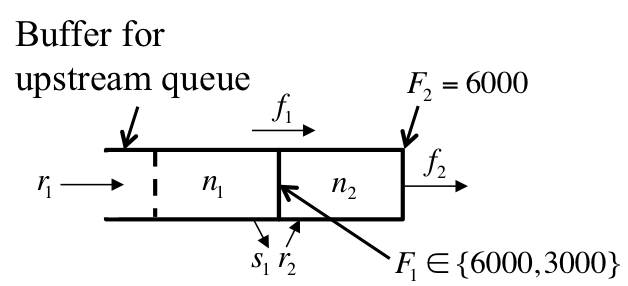
Now we use our results to study the stability of a two-cell SS-CTM as in Figure 2. The deterministic version of this system has been studied by Kurzhanskiy [26].
Refer to caption
Figure 2: A two-cell freeway with a single incident hotspot.

We consider the following stochastic capacity model:

={1,2},F1=[6000,6000]T,F2=[3000,6000]T,formulae-sequence12formulae-sequencesuperscript𝐹1superscript60006000𝑇superscript𝐹2superscript30006000𝑇\displaystyle\mathcal{I}=\{1,2\},{F}^{1}=[6000,6000]^{T},{F}^{2}=[3000,6000]^{T},
λ12=λ21=1[hr1].subscript𝜆12subscript𝜆211delimited-[]superscript𝑟1\displaystyle\lambda_{12}=\lambda_{21}=1[hr^{-1}]. (38)

In words, the SS-CTM has a nominal capacity of 6000 veh/hr (mode 1). Cell 1 is an incident hotspot, whose capacity reduces to 3000 veh/hr during incidents (mode 2). Incidents occur and clear at the rate 1 per hour. The mainline ratios are β1=0.75subscript𝛽10.75\beta_{1}=0.75 and β2=1subscript𝛽21\beta_{2}=1. The inflow is r=[r1,r2]T=02𝑟superscriptsubscript𝑟1subscript𝑟2𝑇superscriptsubscriptabsent02absentr=[r_{1},r_{2}]^{T}\in\mathcal{R}=_{\geq 0}^{2}. Other model parameters are given by Table 1. The steady-state distribution of the mode transition process can be easily obtained: 𝗉1=𝗉2=0.5.subscript𝗉1subscript𝗉20.5\mathsf{p}_{1}=\mathsf{p}_{2}=0.5.

Table 1: Traffic flow parameters in example SS-CTM.
Name Symbol Value unit
Cell length l𝑙l 1 mi
Free-flow speed v𝑣v 60 mi/hr
Congestion wave speed w𝑤w 20 mi/hr
Jam density nmaxsuperscript𝑛{n}^{\max} 400 veh/mi
Critical density ncritsuperscript𝑛critn^{\mathrm{crit}} 100 veh/mi

Our objective is to determine whether the system is stable under given inflow vectors r=[r1,r2]TR𝑟superscriptsubscript𝑟1subscript𝑟2𝑇𝑅r=[r_{1},r_{2}]^{T}\in R. Specifically, we consider two different cases, one being unstable and the other being stable.

1) Consider the inflow vector r=[4320,2400]T𝑟superscript43202400𝑇r=[4320,2400]^{T}.

Refer to caption
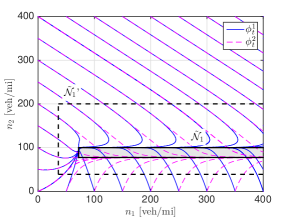
Figure 3: Integral curves and invariant set (shaded area) of the two-cell SS-CTM with r=[4320,2400]T𝑟superscript43202400𝑇r=[4320,2400]^{T}.

Note that the nominal flows given by this r𝑟r do not exceed the average capacities of both cells, i.e. satisfy (25):

r1=4320<0.5(6000)+0.5(3000)=4500[veh/hr],subscript𝑟143200.560000.530004500delimited-[]vehhr\displaystyle r_{1}=4320<0.5(6000)+0.5(3000)=4500[\mathrm{veh/hr}],
0.75r1+r2=0.75(4320)+2400)=5640<6000[veh/hr].\displaystyle 0.75r_{1}+r_{2}=0.75(4320)+2400)=5640<6000[\mathrm{veh/hr}].

However, naïvely concluding stability based on the above observation is incorrect. By computing the invariant set and the spillback-adjusted capacities, and applying Theorem 1, we can conclude that the SS-CTM is in fact unstable. To see this, we first use Proposition 1 to obtain an invariant set

𝒩~1=[72,)×[77.5,100].subscript~𝒩17277.5100\displaystyle\widetilde{\mathcal{N}}_{1}=[72,\infty)\times[77.5,100]. (39)

Figure 3 illustrates that, for the two-dimensional system, all integral curves are attracted to 𝒩~1subscript~𝒩1\widetilde{\mathcal{N}}_{1} and remain within it thereafter (i.e. 𝒩~1subscript~𝒩1\widetilde{\mathcal{N}}_{1} satisfies (18)). In fact, it turns out that 𝒩~1subscript~𝒩1\widetilde{\mathcal{N}}_{1} is the smallest invariant set of the form in (20). Thus, we have

F~11(n¯,r)=4960[veh/hr],superscriptsubscript~𝐹11¯𝑛𝑟4960delimited-[]vehhr\displaystyle\widetilde{F}_{1}^{1}(\underline{n},r)=4960[\mathrm{veh/hr}],
F~21(n¯,r)=3000[veh/hr],superscriptsubscript~𝐹21¯𝑛𝑟3000delimited-[]vehhr\displaystyle\widetilde{F}_{2}^{1}(\underline{n},r)=3000[\mathrm{veh/hr}],
F~21(n¯,r)=F~22(n¯,r)=6000.superscriptsubscript~𝐹21¯𝑛𝑟superscriptsubscript~𝐹22¯𝑛𝑟6000\displaystyle\widetilde{F}_{2}^{1}(\underline{n},r)=\widetilde{F}_{2}^{2}(\underline{n},r)=6000.

We can check that

r1=4320>𝗉1F~11+𝗉2F~12=3980.subscript𝑟14320subscript𝗉1superscriptsubscript~𝐹11subscript𝗉2superscriptsubscript~𝐹123980\displaystyle r_{1}=4320>\mathsf{p}_{1}\widetilde{F}_{1}^{1}+\mathsf{p}_{2}\widetilde{F}_{1}^{2}=3980.

Therefore, by Theorem 1, the system is unstable.

Now, we use this example to show that a smaller invariant set leads to a sharper necessary condition. Consider another set 𝒩=[36,)×[38.75,200]superscript𝒩3638.75200\mathcal{N}^{\prime}=[36,\infty)\times[38.75,200]; see Figure 3 to note that this set is also invariant in the sense of (18). For 𝒩~1subscriptsuperscript~𝒩1\widetilde{\mathcal{N}}^{\prime}_{1}, we have

F~11(n¯,r)=F~21(n¯,r)=F~22(n¯,r)=6000,F~12(n¯,r)=3000.formulae-sequencesuperscriptsubscript~𝐹11superscript¯𝑛𝑟superscriptsubscript~𝐹21superscript¯𝑛𝑟superscriptsubscript~𝐹22superscript¯𝑛𝑟6000superscriptsubscript~𝐹12superscript¯𝑛𝑟3000\displaystyle\widetilde{F}_{1}^{1}(\underline{n}^{\prime},r)=\widetilde{F}_{2}^{1}(\underline{n}^{\prime},r)=\widetilde{F}_{2}^{2}(\underline{n}^{\prime},r)=6000,\;{\widetilde{F}}_{1}^{2}(\underline{n}^{\prime},r)=3000.

Since r1=4320>0.5(6000)+0.5(3000)=4500subscript𝑟143200.560000.530004500r_{1}=4320>0.5(6000)+0.5(3000)=4500, β1r1+r2=56406000subscript𝛽1subscript𝑟1subscript𝑟256406000\beta_{1}r_{1}+r_{2}=5640\leq 6000, the given inflow vector satisfies the necessary condition associated with 𝒩~1subscriptsuperscript~𝒩1\widetilde{\mathcal{N}}^{\prime}_{1}. In other words, using the condition with 𝒩~1subscriptsuperscript~𝒩1\widetilde{\mathcal{N}}^{\prime}_{1}, we cannot conclude the instability of the given inflow vector r𝑟r, while using the condition with 𝒩~1subscript~𝒩1\widetilde{\mathcal{N}}_{1} (as given by (39)) we are able to do so.

2) Now, consider the inflow vector r=[3600,600]T𝑟superscript3600600𝑇r=[3600,600]^{T}.

Refer to caption
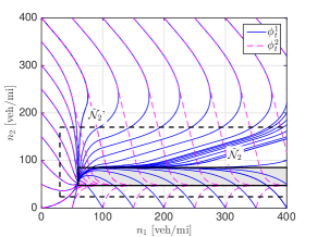
Figure 4: Integral curves and invariant set (shaded area) of the two-cell SS-CTM with r=[3600,600]T𝑟superscript3600600𝑇r=[3600,600]^{T}.

Once again, from Proposition 1, we obtain the following invariant set:

𝒩~2=[60,)×[47.5,85].subscript~𝒩26047.585\displaystyle\widetilde{\mathcal{N}}_{2}=[60,\infty)\times[47.5,85]. (40)

Similar to the previous case, this invariant set is the smallest one that can be written as a Cartesian product of intervals; see Figure 4. Then, we obtain from (22) that

F~11(n¯,r)=6000[veh/hr],F~12(n¯,r)=3000[veh/hr],formulae-sequencesuperscriptsubscript~𝐹11¯𝑛𝑟6000delimited-[]vehhrsuperscriptsubscript~𝐹12¯𝑛𝑟3000delimited-[]vehhr\displaystyle\widetilde{F}_{1}^{1}(\underline{n},r)=6000[\mathrm{veh/hr}],\;\widetilde{F}_{1}^{2}(\underline{n},r)=3000[\mathrm{veh/hr}],
F~21(n¯,r)=F~22(n¯,r)=6000[veh/hr].superscriptsubscript~𝐹21¯𝑛𝑟superscriptsubscript~𝐹22¯𝑛𝑟6000delimited-[]vehhr\displaystyle\widetilde{F}_{2}^{1}(\underline{n},r)=\widetilde{F}_{2}^{2}(\underline{n},r)=6000[\mathrm{veh/hr}].

Note that, the necessary condition (Theorem 1) is satisfied, since

r10.5(6000)+0.5(3000)=4500[veh/hr],subscript𝑟10.560000.530004500delimited-[]vehhr\displaystyle r_{1}\leq 0.5(6000)+0.5(3000)=4500[\mathrm{veh/hr}],
β1r1+r2=33006000[veh/hr],subscript𝛽1subscript𝑟1subscript𝑟233006000delimited-[]vehhr\displaystyle\beta_{1}r_{1}+r_{2}=3300\leq 6000[\mathrm{veh/hr}],

To check the sufficient condition (Theorem 2), we first compute the weights using (27):

γ1=5,γ2=2.22,Γ1=5.42,Γ2=2.22,formulae-sequencesubscript𝛾15formulae-sequencesubscript𝛾22.22formulae-sequencesubscriptΓ15.42subscriptΓ22.22\displaystyle\gamma_{1}=5,\;\gamma_{2}=2.22,\;\Gamma_{1}=5.42,\;\Gamma_{2}=2.22,

which implies

(r)=2.08×10⁴,𝑟2.08superscript104\displaystyle\mathscr{R}(r)=2.08\times 10^{4},
1(n¯,n¯,r)=2.88×104,2(n¯,n¯,r)=1.76×10⁴,formulae-sequencesubscript1¯𝑛¯𝑛𝑟2.88superscript104subscript2¯𝑛¯𝑛𝑟1.76superscript104\displaystyle\mathscr{F}_{1}(\underline{n},\overline{n},r)=2.88\times 10^{4},\;\mathscr{F}_{2}(\underline{n},\overline{n},r)=1.76\times 10^{4},

Then, plugging the numerical values into (31), we obtain

a1b(2.082.88)×104+(a2a1)1,subscript𝑎1𝑏2.082.88superscript104subscript𝑎2subscript𝑎11\displaystyle a_{1}b(2.08-2.88)\times 10^{4}+(a_{2}-a_{1})\leq-1,
a2b(2.081.76)×104+(a1a2)1.subscript𝑎2𝑏2.081.76superscript104subscript𝑎1subscript𝑎21\displaystyle a_{2}b(2.08-1.76)\times 10^{4}+(a_{1}-a_{2})\leq-1.

We can easily obtain a solution to the above bilinear inequalities, one of which is

a1=10,a2=17,b=104.formulae-sequencesubscript𝑎110formulae-sequencesubscript𝑎217𝑏superscript104\displaystyle a_{1}=10,\;a_{2}=17,\;b=10^{-4}.

Hence, we conclude from Theorem 2 that the system is stable in the sense of (17).

Now we show that an invariant set larger than 𝒩~2subscript~𝒩2\widetilde{\mathcal{N}}_{2} (as given by (40)) leads to a weaker sufficient condition. Consider a larger set 𝒩~2=[35,)×[23.75,170]subscriptsuperscript~𝒩23523.75170\widetilde{\mathcal{N}}^{\prime}_{2}=[35,\infty)\times[23.75,170] (see Figure 4), which is also invariant in the sense of (18). With 𝒩~2subscriptsuperscript~𝒩2\widetilde{\mathcal{N}}^{\prime}_{2}, we have

(r)=2.08×10⁴,𝑟2.08superscript104\displaystyle{\mathscr{R}}(r)=2.08\times 10^{4},
1(n¯,n¯,r)=2.57×104,2(n¯,n¯,r)=1.44×10⁴,formulae-sequencesubscript1superscript¯𝑛superscript¯𝑛𝑟2.57superscript104subscript2superscript¯𝑛superscript¯𝑛𝑟1.44superscript104\displaystyle\mathscr{F}_{1}(\underline{n}^{\prime},\overline{n}^{\prime},r)=2.57\times 10^{4},\;\mathscr{F}_{2}(\underline{n}^{\prime},\overline{n}^{\prime},r)=1.44\times 10^{4},

which leads to the sufficient condition that

a1b(0.49)104+(a2a1)1,subscript𝑎1𝑏0.49superscript104subscript𝑎2subscript𝑎11\displaystyle a_{1}b(-0.49)10^{4}+(a_{2}-a_{1})\leq-1,
a2b(0.64)104+(a1a2)1.subscript𝑎2𝑏0.64superscript104subscript𝑎1subscript𝑎21\displaystyle a_{2}b(0.64)10^{4}+(a_{1}-a_{2})\leq-1.

It is not hard to show that the above inequalities have no positive feasible solutions for a1subscript𝑎1a_{1}, a2subscript𝑎2a_{2}, and b𝑏b. Thus, the sufficient condition with 𝒩~2subscriptsuperscript~𝒩2\widetilde{\mathcal{N}}^{\prime}_{2} cannot be used to ensure stability. Hence, the sufficient condition resulting from using 𝒩~2subscript~𝒩2\widetilde{\mathcal{N}}_{2} is sharper than that obtained by using 𝒩~2subscriptsuperscript~𝒩2\widetilde{\mathcal{N}}^{\prime}_{2}.

4 Some Practical Insights

In this section, we derive some practical insights for freeway traffic management under capacity fluctuations. Specifically, we use our results to (i) identify the set of stable inflow vectors for a given capacity model, (ii) analyze the impact due to frequency and intensity of capacity fluctuation on throughput, and (iii) study the effect of correlation between capacity fluctuation at various locations.
Refer to caption
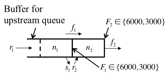
Figure 5: A two-cell freeway with two incident hotspots.
Refer to caption
(a) Baseline model.
Refer to caption
(b) Variant 1.
Refer to caption
(c) Variant 2.
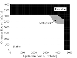
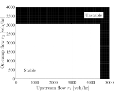
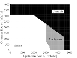
Figure 6: Stability of the two-cell freeway with various inflow vectors r=[r1,r2]T𝑟superscriptsubscript𝑟1subscript𝑟2𝑇r=[r_{1},r_{2}]^{T} determined by Theorems 1 and 2.

A two-cell system as shown in Figure 5 is sufficient for our purpose. Note that this system is distinct from that considered in Section 3.2 in that both cells of this system have stochastic capacities. The parameters for the (baseline) capacity model is as follows:

={1,2,3,4}.1234\displaystyle\mathcal{I}=\{1,2,3,4\}. (41a)
F1=[6000,6000]T,F2=[3000,6000]T,formulae-sequencesuperscript𝐹1superscript60006000𝑇superscript𝐹2superscript30006000𝑇\displaystyle{F}^{1}=[6000,6000]^{T},\;{F}^{2}=[3000,6000]^{T}, (41b)
F3=[6000,3000]T,F4=[3000,3000]T,formulae-sequencesuperscript𝐹3superscript60003000𝑇superscript𝐹4superscript30003000𝑇\displaystyle{F}^{3}=[6000,3000]^{T},\;{F}^{4}=[3000,3000]^{T}, (41c)
Λ=[2110120110210112].Λdelimited-[]2110120110210112\displaystyle\Lambda=\left[\begin{array}[]{cccc}-2&1&1&0\\ 1&-2&0&1\\ 1&0&-2&1\\ 0&1&1&-2\end{array}\right]. (41h)

Note that the transition rate matrix defined above implies that the capacity fluctuations at both cells are mutually independent. (We will discuss about the impact of correlation between cell capacities later.) The remaining parameters for the SS-CTM are given by Table 1.

4.1 Set of stabilizing inflow vectors

For an inflow vector r=[r1,r2]T02𝑟superscriptsubscript𝑟1subscript𝑟2𝑇superscriptsubscriptabsent02absentr=[r_{1},r_{2}]^{T}\in_{\geq 0}^{2}, we know that r𝑟r is unstable if it does not satisfy the necessary condition (Theorem 1), and that r𝑟r is stable if it satisfies the sufficient condition (Theorem 2). For practicality, we also assume that the on-ramp has a fixed saturation rate of 3000 veh/hr. Thus, the on-ramp inflow r2subscript𝑟2r_{2} cannot exceed 3000 veh/hr if the freeway is stable.

Applying our stability conditions to various inflow vectors [r1,r2]Tsuperscriptsubscript𝑟1subscript𝑟2𝑇[r_{1},r_{2}]^{T}, we obtain Figure 6(a). In this figure, the r1subscript𝑟1r_{1}-r2subscript𝑟2r_{2} plane is partitioned into three regions: The “Unstable” region (in black) depicts the set of inflow vectors violating the necessary condition. Thus, any inflow vector in this region leads to an infinite traffic queue. We denote the complement of this region as 1subscript1\mathcal{R}_{1}. The “Stable” region (in white) depicts the set of inflow vectors satisfying sufficient condition. In this example, we solve the bilinear inequalities (31) using YALMIP, a MATLAB-based optimization tool [30]. By Theorem 2, the inflow vectors in this region lead to a traffic queue bounded in the sense of (17). We denote this region as 2subscript2\mathcal{R}_{2}.

Notice that there is a gap, labeled as “Ambiguous”, between the “Stable” and the “Unstable” regions. This region shows the gap between the necessary condition and the sufficient condition; for inflow vectors in this region, our stability conditions do not provide a conclusive answer.

These results can be used to calculate stabilizing inflows that lead to maximum throughput. For a stable inflow vector r𝑟r, we follow [28] and define throughput J(r)𝐽𝑟J(r) of the two-cell system as follows:

J(r)=r1(2l)+r2l=2lr1+lr2.𝐽𝑟subscript𝑟12𝑙subscript𝑟2𝑙2𝑙subscript𝑟1𝑙subscript𝑟2\displaystyle J(r)=r_{1}(2l)+r_{2}l=2lr_{1}+lr_{2}.

One can interpret J(r)𝐽𝑟J(r) as the average vehicle miles traveled per unit time. Let stablesubscriptstable\mathcal{R}_{\mathrm{stable}} be the set of stabilizing inflow vectors. For the given capacity model, we are interested in the maximum throughput Jmaxsubscript𝐽J_{\max}:

Jmax=maxrstable2lr1+lr2subscript𝐽subscript𝑟subscriptstable2𝑙subscript𝑟1𝑙subscript𝑟2\displaystyle J_{\max}=\max_{r\in\mathcal{R}_{\mathrm{stable}}}2lr_{1}+lr_{2}

Since our stability conditions are in general not necessary and sufficient, it is not easy to compute the exact value of Jmaxsubscript𝐽J_{\max}. However, we are able to derive upper and lower bounds for Jmaxsubscript𝐽J_{\max}. Note that 2stable1subscript2subscriptstablesubscript1\mathcal{R}_{2}\subseteq\mathcal{R}_{\mathrm{stable}}\subseteq\mathcal{R}_{1}. Hence, we can obtain an upper bound J¯maxsubscript¯𝐽\overline{J}_{\max} and a lower bound J¯maxsubscript¯𝐽\underline{J}_{\max} for Jmaxsubscript𝐽J_{\max} as follows:

J¯max=maxr1(2lr1+lr2),subscript¯𝐽subscript𝑟subscript12𝑙subscript𝑟1𝑙subscript𝑟2\displaystyle\overline{J}_{\max}=\max_{r\in\mathcal{R}_{1}}(2lr_{1}+lr_{2}),
J¯max=maxr2(2lr1+lr2).subscript¯𝐽subscript𝑟subscript22𝑙subscript𝑟1𝑙subscript𝑟2\displaystyle\underline{J}_{\max}=\max_{r\in\mathcal{R}_{2}}(2lr_{1}+lr_{2}).

For this particular example, we can numerically obtain the following bounds:

7170Jmax8910[veh-mi/hr].7170subscript𝐽8910delimited-[]veh-mi/hr\displaystyle 7170\leq J_{\max}\leq 8910[\mbox{veh-mi/hr}]. (42)

Next, to illustrate how model characteristics affect the size of the “Ambiguous” region, we consider the following variants of the baseline model specified by (41):

  1. 1.

    Cell 2 is no longer an incident hotspot; i.e. F2i=6000superscriptsubscript𝐹2𝑖6000F_{2}^{i}=6000 veh/hr for all i{1,2,3,4}𝑖1234i\in\{1,2,3,4\}.

  2. 2.

    Cell 2 is no longer an incident hotspot, and its capacity is doubled; i.e. F2i=12000superscriptsubscript𝐹2𝑖12000F_{2}^{i}=12000 veh/hr for all i{1,2,3,4}𝑖1234i\in\{1,2,3,4\}.

Compared to the baseline model, both variants has fewer incident hotspots; furthermore, variant 2 has a sufficiently large capacity of cell 2 to prevent spillback between cells 1 and 2. Hence, we can sort the three models in the order of “decreasing complexity” as follows: baseline, variant 1, variant 2.

By comparing Figures 6(a)6(c), we can see that the gap between the sufficient condition and the necessary condition reduces as the model complexity reduces. In addition, for variant 2, as shown in Figure 6(c), the ambiguous region vanishes; i.e. the two-cell freeway is stable if and only if the inflows are less than average capacities (r1<4500subscript𝑟14500r_{1}<4500 veh/hr, r2<3000subscript𝑟23000r_{2}<3000 veh/hr.)444In fact, for this simple example, one can prove this statement by explicitly constructing aisubscript𝑎𝑖a_{i} and b𝑏b in the Lyapunov function under this condition.

4.2 Impact of capacity fluctuation on throughput

Now we estimate the maximum throughput that can be achieved under a class of capacity models parameterized by ΔFΔ𝐹\Delta F and λ𝜆\lambda as follows:

={1,2,3,4}.1234\displaystyle\mathcal{I}=\{1,2,3,4\}.
F1=[6000,6000]T,F2=[6000ΔF,6000]T,formulae-sequencesuperscript𝐹1superscript60006000𝑇superscript𝐹2superscript6000Δ𝐹6000𝑇\displaystyle{F}^{1}=[6000,6000]^{T},\;{F}^{2}=[6000-\Delta{F},6000]^{T},
F3=[6000,6000ΔF]T,superscript𝐹3superscript60006000Δ𝐹𝑇\displaystyle{F}^{3}=[6000,6000-\Delta{F}]^{T},
F4=[6000ΔF,6000ΔF]T,superscript𝐹4superscript6000Δ𝐹6000Δ𝐹𝑇\displaystyle{F}^{4}=[6000-\Delta{F},6000-\Delta{F}]^{T},
Λ=[2λλλ01(1+λ)0λ10(1+λ)λ0112].Λdelimited-[]2𝜆𝜆𝜆011𝜆0𝜆101𝜆𝜆0112\displaystyle\Lambda=\left[\begin{array}[]{cccc}-2\lambda&\lambda&\lambda&0\\ 1&-(1+\lambda)&0&\lambda\\ 1&0&-(1+\lambda)&\lambda\\ 0&1&1&-2\end{array}\right].

By varying the parameters ΔFΔ𝐹\Delta F and λ𝜆\lambda, we can study the effect the intensity and the frequency of capacity fluctuations on the maximum throughput of SS-CTM.
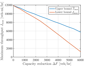
Refer to caption
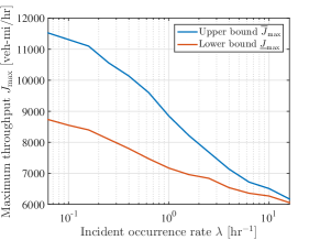
(a) Throughput decreases as incident frequency increases, with ΔFΔ𝐹\Delta F fixed at 300030003000 veh/hr.
Refer to caption
(b) Throughput decreases as incident intensity increases, with λ𝜆\lambda fixed at 1 per hour.
Figure 7: Relation between maximum throughput and incident frequency/intensity. The upper (resp. lower) bounds result from Theorem 1 (resp. Theorem 2).

For various (λ,ΔF)𝜆Δ𝐹(\lambda,\Delta{F}) pairs, we numerically determine J¯maxsubscript¯𝐽\overline{J}_{\max} and J¯maxsubscript¯𝐽\underline{J}_{\max}. Figure 7(a) shows that, with ΔFΔ𝐹\Delta{F} fixed at 3000 veh/hr, J¯maxsubscript¯𝐽\overline{J}_{\max} and J¯maxsubscript¯𝐽\underline{J}_{\max} decreases as λ𝜆\lambda increases. This is intuitive: more frequent capacity disruptions leads to lower throughput. Figure 7(b) shows that, with λ𝜆\lambda fixed at 1 per hr, J¯maxsubscript¯𝐽\overline{J}_{\max} and J¯maxsubscript¯𝐽\underline{J}_{\max} decreases as ΔFΔ𝐹\Delta{F} increases. This is also intuitive: larger capacity reduction leads to lower throughput.

Note that the throughput tends to be more sensitive to ΔFΔ𝐹\Delta{F} than to λ𝜆\lambda. Indeed, as shown in Figure 7(a), if λ𝜆\lambda is doubled from 1 (the baseline) to 2 per hr, the upper (resp. lower) bound is reduced by 7% (resp. 3%). However, if ΔFΔ𝐹\Delta{F} is doubled from 3000 (the baseline) to 6000 veh/hr, we can observe from Figure 7(b) that the upper (resp. lower) bound is reduced by 35% (resp. 82%).

The gap between J¯maxsubscript¯𝐽\overline{J}_{\max} and J¯maxsubscript¯𝐽\underline{J}_{\max} in Figures 7(a) and 7(b) result from the gap between the necessary condition and the sufficient condition for stability.

4.3 Impact of correlated capacity fluctuation

So far we have assumed that the cell capacities in the two-cell freeway are independent. Now we consider the case where the cells’ capacities are correlated. We consider two extreme cases as follows.

Case 1: Suppose that the capacities of both cells are identical for all t0𝑡0t\geq 0. In other words, the freeway has two modes {1,2}12\{1,2\} associated with F1=[6000,6000]Tsuperscript𝐹1superscript60006000𝑇{F}^{1}=[6000,6000]^{T} and F2=[3000,3000]Tsuperscript𝐹2superscript30003000𝑇{F}^{2}=[3000,3000]^{T}. In this case, the transition matrix is

ΛCase 1=[1111].subscriptΛCase1delimited-[]1111\displaystyle\Lambda_{\mathrm{Case\,1}}=\left[\begin{array}[]{cc}-1&1\\ 1&-1\end{array}\right].

By implementing Theorems 1 and 2, we obtain the following bounds for the maximum throughput:

7485Jmax8910[veh-mi/hr].7485subscript𝐽8910[veh-mi/hr]\displaystyle 7485\leq J_{\max}\leq 8910\mbox{[veh-mi/hr]}.

The upper bounds is the same as that in (42), since the necessary condition (25) only involves the spillback-adjusted capacities of individual cells but does not depend on the correlation between cells. However, the lower bound (obtained from the sufficient condition) is higher compared to that in (42).

Case 2: Suppose that the freeway always has exactly one incident in either cell. In other words, the freeway has two modes {1,2}12\{1,2\} associated with F1=[6000,3000]Tsuperscript𝐹1superscript60003000𝑇{F}^{1}=[6000,3000]^{T} and F2=[6000,3000]Tsuperscript𝐹2superscript60003000𝑇{F}^{2}=[6000,3000]^{T}. In this case, the transition matrix is

ΛCase 2=[1111].subscriptΛCase2delimited-[]1111\displaystyle\Lambda_{\mathrm{Case\,2}}=\left[\begin{array}[]{cc}-1&1\\ 1&-1\end{array}\right].

By implementing Theorems 1 and 2, we obtain the following bounds for the maximum throughput:

6720Jmax8910[veh-mi/hr].6720subscript𝐽8910[veh-mi/hr]\displaystyle 6720\leq J_{\max}\leq 8910\mbox{[veh-mi/hr]}.

In this case, the lower bound is lower than that in the benchmark case (42).

In conclusion, even with the same cell average cell capacities (4500 veh/hr for both cells), the freeway’s maximum throughput estimated by the sufficient condition could vary (in the order of 10%) due to spatial correlation. Therefore, compared to traditional approaches that assume independent cell capacities (e.g. [39]), our approach is able to capture the effect of spatial correlation and possibly achieve better throughput. In a related work [20], we have found that the extent of spatial correlation can be quite significant in practice.

We finally note that, in some situations, the transition rate matrix ΛΛ\Lambda may not be easy to calibrate. Analysis of the SS-CTM with partially known transition rates is indeed a practically relevant question, but is beyond the scope of this paper. We refer the readers to [40] for more information on stochastic switching systems with partially known transition probabilities.

5 Concluding Remarks

The main contributions of this article are: (i) a stochastic switching cell transmission model for traffic dynamics in incident-prone freeways and (ii) easily checkable stability conditions for the SS-CTM (Theorems 1 and 2). A sufficient condition for stability is that the inflow does not exceed the spillback-adjusted capacity. A necessary condition for stability is that a set of bilinear inequalities, which is derived from the Foster-Lyapunov drift condition, admit positive solutions. Both conditions build on a construction of a globally attracting and invariant set of the SS-CTM (Proposition 1). Using these results, we derive new insights for the impact of capacity fluctuation on the upstream traffic queue length and the attainable throughput.

Our work can be extended in several directions. First, with a different (or more sophisticated) choice of Lyapunov function or a tighter invariant set, the stability conditions may be further refined. Second, estimation methods for the SS-CTM can be developed based on previous work such as [20, 13]. Third, recent results on network traffic flow models [19, 9, 8] makes possible the extension of our model and method to the network setting, and to feedback-controlled systems.

Appendix
Proofs of Main Results

.1 Proof of Proposition 1

.1.1 Invariant

To show the invariance of 𝒩~~𝒩\widetilde{\mathcal{N}}, we demonstrate that the vector field G𝐺G points towards the interior of 𝒩~~𝒩\widetilde{\mathcal{N}} everywhere on the boundary of 𝒩~~𝒩\widetilde{\mathcal{N}}. That is, for each n𝒩~𝑛~𝒩{n}\in\widetilde{\mathcal{N}} such that nk=n¯ksubscript𝑛𝑘subscript¯𝑛𝑘{n}_{k}=\underline{n}_{k} (resp. nk=n¯ksubscript𝑛𝑘subscript¯𝑛𝑘{n}_{k}=\overline{n}_{k}) for some k{1,,K}𝑘1𝐾k\in\{1,\ldots,K\} (resp. k{2,,K}𝑘2𝐾k\in\{2,\ldots,K\}), we have Gk(i,n,r)0subscript𝐺𝑘𝑖𝑛𝑟0G_{k}(i,{n},r)\geq 0 (resp. Gk(i,n,r)0subscript𝐺𝑘𝑖𝑛𝑟0G_{k}(i,{n},r)\leq 0) for all i𝑖i\in\mathcal{I}.

a) We first study the directionality of the vector field on the lower boundaries. Consider a given r𝑟r\in\mathcal{R}.

a.1) For each n𝒩~𝑛~𝒩{n}\in\widetilde{\mathcal{N}} such that n1=n¯1subscript𝑛1subscript¯𝑛1{n}_{1}=\underline{n}_{1}, we have

G1(i,n,r)subscript𝐺1𝑖𝑛𝑟\displaystyle G_{1}(i,{n},r) =(13a)r1f1(i,n¯1,n2,r2)/β1superscriptitalic-(13aitalic-)absentsubscript𝑟1subscript𝑓1𝑖subscript¯𝑛1subscript𝑛2subscript𝑟2subscript𝛽1\displaystyle\stackrel{{\scriptstyle\footnotesize\eqref{Eq_G1}}}{{=}}r_{1}-f_{1}(i,\underline{n}_{1},{n}_{2},r_{2})/\beta_{1}
=(11b)r1min{vn¯1,F1i,(R2(n2)r2)+/β2}superscriptitalic-(11bitalic-)absentsubscript𝑟1𝑣subscript¯𝑛1superscriptsubscript𝐹1𝑖subscriptsubscript𝑅2subscript𝑛2subscript𝑟2subscript𝛽2\displaystyle\stackrel{{\scriptstyle\footnotesize\eqref{Eq_fk}}}{{=}}r_{1}-\min\left\{v\underline{n}_{1},{F}_{1}^{i},(R_{2}({n}_{2})-r_{2})_{+}/\beta_{2}\right\}
r1vn¯1(21a)r1vr1v=0,i.formulae-sequenceabsentsubscript𝑟1𝑣subscript¯𝑛1superscriptitalic-(21aitalic-)subscript𝑟1𝑣subscript𝑟1𝑣0for-all𝑖\displaystyle\geq r_{1}-v\underline{n}_{1}\stackrel{{\scriptstyle\footnotesize\eqref{Eq_rhobot1}}}{{\geq}}r_{1}-v\frac{r_{1}}{v}=0,\quad\forall i\in\mathcal{I}. (43)

a.2) For each n𝒩~𝑛~𝒩{n}\in\widetilde{\mathcal{N}} such that nk=n¯ksubscript𝑛𝑘subscript¯𝑛𝑘{n}_{k}=\underline{n}_{k} for some k{2,,K1}𝑘2𝐾1k\in\{2,\ldots,K-1\}, we need to show that Gk0subscript𝐺𝑘0G_{k}\geq 0.

First, note that

fk1(i,nk1,n¯k,rk)subscript𝑓𝑘1𝑖subscript𝑛𝑘1subscript¯𝑛𝑘subscript𝑟𝑘\displaystyle f_{k-1}\left(i,{n}_{k-1},\underline{n}_{k},r_{k}\right)
=(11b)min{βk1vnk1,βk1Fk1i,Rk(n¯k)rk}superscriptitalic-(11bitalic-)absentsubscript𝛽𝑘1𝑣subscript𝑛𝑘1subscript𝛽𝑘1superscriptsubscript𝐹𝑘1𝑖subscript𝑅𝑘subscript¯𝑛𝑘subscript𝑟𝑘\displaystyle\stackrel{{\scriptstyle\footnotesize\eqref{Eq_fk}}}{{=}}\min\left\{\beta_{k-1}v{n}_{k-1},\beta_{k-1}{F}_{k-1}^{i},R_{k}(\underline{n}_{k})-r_{k}\right\}
min{βk1vn¯k1,βk1Fk1i,Rk(n¯k)rk}absentsubscript𝛽𝑘1𝑣subscript¯𝑛𝑘1subscript𝛽𝑘1superscriptsubscript𝐹𝑘1𝑖subscript𝑅𝑘subscript¯𝑛𝑘subscript𝑟𝑘\displaystyle\geq\min\left\{\beta_{k-1}v\underline{n}_{k-1},\beta_{k-1}{F}_{k-1}^{i},R_{k}(\underline{n}_{k})-r_{k}\right\}
(9b)(21b)min{vn¯krk,w(nmaxn¯k)rk}superscriptitalic-(9bitalic-)italic-(21bitalic-)absent𝑣subscript¯𝑛𝑘subscript𝑟𝑘𝑤superscript𝑛subscript¯𝑛𝑘subscript𝑟𝑘\displaystyle\stackrel{{\scriptstyle\footnotesize\eqref{Eq_Receiving}\eqref{Eq_rhobotk}}}{{\geq}}\min\left\{{v}\underline{n}_{k}-r_{k},w({n}^{\max}-\underline{n}_{k})-r_{k}\right\} (44)

Since n¯k(21b)Fkmax/v,superscriptitalic-(21bitalic-)subscript¯𝑛𝑘superscriptsubscript𝐹𝑘𝑣\underline{n}_{k}\stackrel{{\scriptstyle\footnotesize\eqref{Eq_rhobotk}}}{{\leq}}{F}_{k}^{\max}/v, we can obtain from (10) that

vn¯kw(nmaxn¯k).𝑣subscript¯𝑛𝑘𝑤superscript𝑛subscript¯𝑛𝑘\displaystyle{v}\underline{n}_{k}\leq w\left({n}^{\max}-\underline{n}_{k}\right).

Plugging the above into (44), we obtain

fk1(i,nk1,n¯k,rk)vn¯krk.subscript𝑓𝑘1𝑖subscript𝑛𝑘1subscript¯𝑛𝑘subscript𝑟𝑘𝑣subscript¯𝑛𝑘subscript𝑟𝑘\displaystyle f_{k-1}\left(i,{n}_{k-1},\underline{n}_{k},r_{k}\right)\geq{v}\underline{n}_{k}-r_{k}. (45)

Next, note that

fk(i,n¯k,nk+1,rk+1)/βksubscript𝑓𝑘𝑖subscript¯𝑛𝑘subscript𝑛𝑘1subscript𝑟𝑘1subscript𝛽𝑘\displaystyle f_{k}\left(i,\underline{n}_{k},{n}_{k+1},r_{k+1}\right)/\beta_{k}
=(11b)min{vn¯k,Fki,w(nmaxnk+1)rkβk}vn¯k.superscriptitalic-(11bitalic-)absent𝑣subscript¯𝑛𝑘superscriptsubscript𝐹𝑘𝑖𝑤superscript𝑛subscript𝑛𝑘1subscript𝑟𝑘subscript𝛽𝑘𝑣subscript¯𝑛𝑘\displaystyle\stackrel{{\scriptstyle\footnotesize\eqref{Eq_fk}}}{{=}}\min\left\{v\underline{n}_{k},{F}_{k}^{i},\frac{w\left({n}^{\max}-{n}_{k+1}\right)-r_{k}}{\beta_{k}}\right\}\leq v\underline{n}_{k}. (46)

Hence, we have

Gk(i,n,k)subscript𝐺𝑘𝑖𝑛𝑘\displaystyle G_{k}(i,{n},k)
=fk1(i,nk1,n¯k,rk)+rkfk(i,n¯k,nk+1,rk+1)/βkabsentsubscript𝑓𝑘1𝑖subscript𝑛𝑘1subscript¯𝑛𝑘subscript𝑟𝑘subscript𝑟𝑘subscript𝑓𝑘𝑖subscript¯𝑛𝑘subscript𝑛𝑘1subscript𝑟𝑘1subscript𝛽𝑘\displaystyle=f_{k-1}\left(i,{n}_{k-1},\underline{n}_{k},r_{k}\right)+r_{k}-f_{k}\left(i,\underline{n}_{k},{n}_{k+1},r_{k+1}\right)/\beta_{k}
(45)(46)vn¯krk+rkvn¯k=0,i.formulae-sequencesuperscriptitalic-(45italic-)italic-(46italic-)absent𝑣subscript¯𝑛𝑘subscript𝑟𝑘subscript𝑟𝑘𝑣subscript¯𝑛𝑘0for-all𝑖\displaystyle\stackrel{{\scriptstyle\footnotesize\eqref{Eq_fk-1<=vrho}\eqref{Eq_fk<=vrhok}}}{{\geq}}{v}\underline{n}_{k}-r_{k}+r_{k}-v\underline{n}_{k}=0,\quad\forall i\in\mathcal{I}. (47)

a.3) The proof for k=K𝑘𝐾k=K is analogous.

b) Next, we study the directionality of the vector field G𝐺G on the upper boundaries. Again, consider a given r𝑟r\in\mathcal{R}.

b.1) For each n𝒩~𝑛~𝒩{n}\in\widetilde{\mathcal{N}} such that nK=n¯Ksubscript𝑛𝐾subscript¯𝑛𝐾{n}_{K}=\overline{n}_{K}, we need to consider the two subcases in (21e):

If βK1Fmax+rKFKminsubscript𝛽𝐾1superscript𝐹subscript𝑟𝐾superscriptsubscript𝐹𝐾\beta_{K-1}{F}^{\max}+r_{K}\leq{F}_{K}^{\min}, then we have

fK1(i,nK1,n¯K,rK)subscript𝑓𝐾1𝑖subscript𝑛𝐾1subscript¯𝑛𝐾subscript𝑟𝐾\displaystyle f_{K-1}(i,{n}_{K-1},\overline{n}_{K},r_{K})
=(11b)min{βK1vnK1,βK1FK1i,w(nmaxn¯K)rK}superscriptitalic-(11bitalic-)absentsubscript𝛽𝐾1𝑣subscript𝑛𝐾1subscript𝛽𝐾1superscriptsubscript𝐹𝐾1𝑖𝑤superscript𝑛subscript¯𝑛𝐾subscript𝑟𝐾\displaystyle\stackrel{{\scriptstyle\footnotesize\eqref{Eq_fk}}}{{=}}\min\{\beta_{K-1}v{n}_{K-1},\beta_{K-1}{F}_{K-1}^{i},w({n}^{\max}-\overline{n}_{K})-r_{K}\}
βK1FK1iβK1Fmax,absentsubscript𝛽𝐾1superscriptsubscript𝐹𝐾1𝑖subscript𝛽𝐾1superscript𝐹\displaystyle\leq\beta_{K-1}F_{K-1}^{i}\leq\beta_{K-1}{F}^{\max}, (48a)
fK(i,n¯K)βK=(11c)min{vn¯K,FKi}=(21e)βK1Fmax+rK.superscriptitalic-(11citalic-)subscript𝑓𝐾𝑖subscript¯𝑛𝐾subscript𝛽𝐾𝑣subscript¯𝑛𝐾superscriptsubscript𝐹𝐾𝑖superscriptitalic-(21eitalic-)subscript𝛽𝐾1superscript𝐹subscript𝑟𝐾\displaystyle\frac{f_{K}(i,\overline{n}_{K})}{\beta_{K}}\stackrel{{\scriptstyle\footnotesize\eqref{Eq_fn}}}{{=}}\min\{v\overline{n}_{K},{F}_{K}^{i}\}\stackrel{{\scriptstyle\footnotesize\eqref{Eq_rhotopn}}}{{=}}\beta_{K-1}{F}^{\max}+r_{K}. (48b)

Thus, we have

GK(i,n,r)=(13c)fK1(i,nK1,n¯K,rK)+rKfK(iK,n¯K)βKsuperscriptitalic-(13citalic-)subscript𝐺𝐾𝑖𝑛𝑟subscript𝑓𝐾1𝑖subscript𝑛𝐾1subscript¯𝑛𝐾subscript𝑟𝐾subscript𝑟𝐾subscript𝑓𝐾subscript𝑖𝐾subscript¯𝑛𝐾subscript𝛽𝐾\displaystyle G_{K}(i,{n},r)\stackrel{{\scriptstyle\footnotesize\eqref{Eq_Gn}}}{{=}}f_{K-1}(i,{n}_{K-1},\overline{n}_{K},r_{K})+r_{K}-\frac{f_{K}(i_{K},\overline{n}_{K})}{\beta_{K}}
(48)βK1Fmax+rK(βK1Fmax+rK)=0,i.formulae-sequencesuperscriptitalic-(48italic-)absentsubscript𝛽𝐾1superscript𝐹subscript𝑟𝐾subscript𝛽𝐾1superscript𝐹subscript𝑟𝐾0for-all𝑖\displaystyle\stackrel{{\scriptstyle\footnotesize\eqref{Eq_fn-1fn}}}{{\leq}}\beta_{K-1}{F}^{\max}+r_{K}-(\beta_{K-1}{F}^{\max}+r_{K})=0,\quad\forall i\in\mathcal{I}.

Otherwise, we have

fK1(i,nK1,n¯K,rK)(11b)w(nmaxn¯K)rKsuperscriptitalic-(11bitalic-)subscript𝑓𝐾1𝑖subscript𝑛𝐾1subscript¯𝑛𝐾subscript𝑟𝐾𝑤superscript𝑛subscript¯𝑛𝐾subscript𝑟𝐾\displaystyle f_{K-1}(i,{n}_{K-1},\overline{n}_{K},r_{K})\stackrel{{\scriptstyle\footnotesize\eqref{Eq_fk}}}{{\leq}}w({n}^{\max}-\overline{n}_{K})-r_{K}
=(21e)FKminrK,superscriptitalic-(21eitalic-)absentsuperscriptsubscript𝐹𝐾subscript𝑟𝐾\displaystyle\stackrel{{\scriptstyle\footnotesize\eqref{Eq_rhotopn}}}{{=}}{F}_{K}^{\min}-r_{K}, (49a)
fK(iK,n¯K)/βK=(11c)(21e)min{v(nmaxFKmin/w),FKi}superscriptitalic-(11citalic-)italic-(21eitalic-)subscript𝑓𝐾subscript𝑖𝐾subscript¯𝑛𝐾subscript𝛽𝐾𝑣superscript𝑛superscriptsubscript𝐹𝐾𝑤superscriptsubscript𝐹𝐾𝑖\displaystyle f_{K}(i_{K},\overline{n}_{K})/\beta_{K}\stackrel{{\scriptstyle\footnotesize\eqref{Eq_fn}\eqref{Eq_rhotopn}}}{{=}}\min\{v({n}^{\max}-{F}_{K}^{\min}/w),{F}_{K}^{i}\}
=(10)FKiFKmin.superscriptitalic-(10italic-)absentsuperscriptsubscript𝐹𝐾𝑖superscriptsubscript𝐹𝐾\displaystyle\stackrel{{\scriptstyle\footnotesize\eqref{Eq_Sbarmax}}}{{=}}{F}_{K}^{i}\geq{F}_{K}^{\min}. (49b)

Thus, we have

GK(i,n,r)=(13c)fK1(i,nK1,n¯K,rK)+rKfK(iK,n¯K)βKsuperscriptitalic-(13citalic-)subscript𝐺𝐾𝑖𝑛𝑟subscript𝑓𝐾1𝑖subscript𝑛𝐾1subscript¯𝑛𝐾subscript𝑟𝐾subscript𝑟𝐾subscript𝑓𝐾subscript𝑖𝐾subscript¯𝑛𝐾subscript𝛽𝐾\displaystyle G_{K}(i,{n},r)\stackrel{{\scriptstyle\footnotesize\eqref{Eq_Gn}}}{{=}}f_{K-1}(i,{n}_{K-1},\overline{n}_{K},r_{K})+r_{K}-\frac{f_{K}(i_{K},\overline{n}_{K})}{\beta_{K}}
(49)(FKminrK)+rKFKmin=0,i.formulae-sequencesuperscriptitalic-(49italic-)absentsuperscriptsubscript𝐹𝐾subscript𝑟𝐾subscript𝑟𝐾superscriptsubscript𝐹𝐾0for-all𝑖\displaystyle\stackrel{{\scriptstyle\footnotesize\eqref{Eq_P1b1}}}{{\leq}}({F}_{K}^{\min}-r_{K})+r_{K}-{F}_{K}^{\min}=0,\quad\forall i\in\mathcal{I}.

b.2) For n𝒩~𝑛~𝒩{n}\in\widetilde{\mathcal{N}} such that nk=n¯ksubscript𝑛𝑘subscript¯𝑛𝑘{n}_{k}=\overline{n}_{k} for some k{1,,K1}𝑘1𝐾1k\in\{1,\ldots,K-1\}, we again need to consider both cases indicated in (21k):

If βk1Fmax+rkmin{Fkmin,Rk+1(n¯k+1)rk+1βk}subscript𝛽𝑘1superscript𝐹subscript𝑟𝑘superscriptsubscript𝐹𝑘subscript𝑅𝑘1subscript¯𝑛𝑘1subscript𝑟𝑘1subscript𝛽𝑘\beta_{k-1}{F}^{\max}+r_{k}\leq\min\{{F}_{k}^{\min},\frac{R_{k+1}(\overline{n}_{k+1})-r_{k+1}}{\beta_{k}}\}, then we have

fk1(i,nk1,n¯k,rk)βk1Fk1iβk1Fmax,subscript𝑓𝑘1𝑖subscript𝑛𝑘1subscript¯𝑛𝑘subscript𝑟𝑘subscript𝛽𝑘1superscriptsubscript𝐹𝑘1𝑖subscript𝛽𝑘1superscript𝐹\displaystyle f_{k-1}(i,{n}_{k-1},\overline{n}_{k},r_{k})\leq\beta_{k-1}F_{k-1}^{i}\leq\beta_{k-1}{F}^{\max}, (50a)
fk(i,n¯k,nk+1,rk+1)/βksubscript𝑓𝑘𝑖subscript¯𝑛𝑘subscript𝑛𝑘1subscript𝑟𝑘1subscript𝛽𝑘\displaystyle f_{k}(i,\overline{n}_{k},{n}_{k+1},r_{k+1})/\beta_{k}
=(11b)min{vn¯k,Fki,w(nmaxnk+1)rk+1βk}superscriptitalic-(11bitalic-)absent𝑣subscript¯𝑛𝑘superscriptsubscript𝐹𝑘𝑖𝑤superscript𝑛subscript𝑛𝑘1subscript𝑟𝑘1subscript𝛽𝑘\displaystyle\stackrel{{\scriptstyle\footnotesize\eqref{Eq_fk}}}{{=}}\min\left\{v\overline{n}_{k},{F}_{k}^{i},\frac{w({n}^{\max}-{n}_{k+1})-r_{k+1}}{\beta_{k}}\right\}
min{vn¯k,Fki,w(nmaxn¯k+1)rk+1βk}absent𝑣subscript¯𝑛𝑘superscriptsubscript𝐹𝑘𝑖𝑤superscript𝑛subscript¯𝑛𝑘1subscript𝑟𝑘1subscript𝛽𝑘\displaystyle\geq\min\left\{v\overline{n}_{k},{F}_{k}^{i},\frac{w({n}^{\max}-\overline{n}_{k+1})-r_{k+1}}{\beta_{k}}\right\}
=(21k)min{βk1Fmax+rk,Fki,w(nmaxn¯k+1)rk+1βk}superscriptitalic-(21kitalic-)absentsubscript𝛽𝑘1superscript𝐹subscript𝑟𝑘superscriptsubscript𝐹𝑘𝑖𝑤superscript𝑛subscript¯𝑛𝑘1subscript𝑟𝑘1subscript𝛽𝑘\displaystyle\stackrel{{\scriptstyle\footnotesize\eqref{Eq_rhotopk}}}{{=}}\min\left\{\beta_{k-1}{F}^{\max}+r_{k},{F}_{k}^{i},\frac{w({n}^{\max}-\overline{n}_{k+1})-r_{k+1}}{\beta_{k}}\right\}
=βk1Fmax+rkabsentsubscript𝛽𝑘1superscript𝐹subscript𝑟𝑘\displaystyle{=}\beta_{k-1}{F}^{\max}+r_{k} (50b)

Thus, we have

Gk(i,n,r)subscript𝐺𝑘𝑖𝑛𝑟\displaystyle G_{k}(i,{n},r)
=fk1(ik1,nk1,n¯k,rk)+rkfk(i,n¯k,nk+1,rk+1)/βkabsentsubscript𝑓𝑘1subscript𝑖𝑘1subscript𝑛𝑘1subscript¯𝑛𝑘subscript𝑟𝑘subscript𝑟𝑘subscript𝑓𝑘𝑖subscript¯𝑛𝑘subscript𝑛𝑘1subscript𝑟𝑘1subscript𝛽𝑘\displaystyle=f_{k-1}(i_{k-1},{n}_{k-1},\overline{n}_{k},r_{k})+r_{k}-f_{k}(i,\overline{n}_{k},{n}_{k+1},r_{k+1})/\beta_{k}
(50)βk1Fmax+rk(βk1Fmax+rk)=0,i.formulae-sequencesuperscriptitalic-(50italic-)absentsubscript𝛽𝑘1superscript𝐹subscript𝑟𝑘subscript𝛽𝑘1superscript𝐹subscript𝑟𝑘0for-all𝑖\displaystyle\stackrel{{\scriptstyle\footnotesize\eqref{Eq_b2}}}{{\leq}}\beta_{k-1}{F}^{\max}+r_{k}-(\beta_{k-1}{F}^{\max}+r_{k})=0,\quad\forall i\in\mathcal{I}.

Otherwise, we have

fk1(i,nk1,n¯k,rk)w(nmaxn¯k)rksubscript𝑓𝑘1𝑖subscript𝑛𝑘1subscript¯𝑛𝑘subscript𝑟𝑘𝑤superscript𝑛subscript¯𝑛𝑘subscript𝑟𝑘\displaystyle f_{k-1}(i,{n}_{k-1},\overline{n}_{k},r_{k})\leq w({n}^{\max}-\overline{n}_{k})-r_{k}
=(21k)min{Fkmin,w(nmaxn¯k+1)rk+1βk}rk,superscriptitalic-(21kitalic-)absentsuperscriptsubscript𝐹𝑘𝑤superscript𝑛subscript¯𝑛𝑘1subscript𝑟𝑘1subscript𝛽𝑘subscript𝑟𝑘\displaystyle\stackrel{{\scriptstyle\footnotesize\eqref{Eq_rhotopk}}}{{=}}\min\left\{{F}_{k}^{\min},\frac{w({n}^{\max}-\overline{n}_{k+1})-r_{k+1}}{\beta_{k}}\right\}-r_{k}, (51a)
fk(i,n¯k,nk+1,rk+1)/βKsubscript𝑓𝑘𝑖subscript¯𝑛𝑘subscript𝑛𝑘1subscript𝑟𝑘1subscript𝛽𝐾\displaystyle f_{k}(i,\overline{n}_{k},{n}_{k+1},r_{k+1})/\beta_{K}
=min{vn¯k,Fki,w(nmaxnk+1)rk+1βk}absent𝑣subscript¯𝑛𝑘superscriptsubscript𝐹𝑘𝑖𝑤superscript𝑛subscript𝑛𝑘1subscript𝑟𝑘1subscript𝛽𝑘\displaystyle=\min\left\{v\overline{n}_{k},{F}_{k}^{i},\frac{w({n}^{\max}-{n}_{k+1})-r_{k+1}}{\beta_{k}}\right\}
min{vn¯k,Fki,w(nmaxn¯k+1)rk+1βk}absent𝑣subscript¯𝑛𝑘superscriptsubscript𝐹𝑘𝑖𝑤superscript𝑛subscript¯𝑛𝑘1subscript𝑟𝑘1subscript𝛽𝑘\displaystyle\geq\min\left\{v\overline{n}_{k},{F}_{k}^{i},\frac{w({n}^{\max}-\overline{n}_{k+1})-r_{k+1}}{\beta_{k}}\right\}
=(21k)min{Fki,w(nmaxn¯k+1)rk+1βk}superscriptitalic-(21kitalic-)absentsuperscriptsubscript𝐹𝑘𝑖𝑤superscript𝑛subscript¯𝑛𝑘1subscript𝑟𝑘1subscript𝛽𝑘\displaystyle\stackrel{{\scriptstyle\footnotesize\eqref{Eq_rhotopk}}}{{=}}\min\left\{{F}_{k}^{i},\frac{w({n}^{\max}-\overline{n}_{k+1})-r_{k+1}}{\beta_{k}}\right\}
min{Fkmin,w(nmaxn¯k+1)rk+1βk}.absentsuperscriptsubscript𝐹𝑘𝑤superscript𝑛subscript¯𝑛𝑘1subscript𝑟𝑘1subscript𝛽𝑘\displaystyle\geq\min\left\{{F}_{k}^{\min},\frac{w({n}^{\max}-\overline{n}_{k+1})-r_{k+1}}{\beta_{k}}\right\}. (51b)

Thus, we have

Gk(i,n,r)=fk1(i,nk1,n¯k,rk)+rksubscript𝐺𝑘𝑖𝑛𝑟subscript𝑓𝑘1𝑖subscript𝑛𝑘1subscript¯𝑛𝑘subscript𝑟𝑘subscript𝑟𝑘\displaystyle G_{k}(i,{n},r)=f_{k-1}(i,{n}_{k-1},\overline{n}_{k},r_{k})+r_{k}
fk(ik,n¯k,nk+1,rk+1)/βk(51)0,i.formulae-sequencesuperscriptitalic-(51italic-)subscript𝑓𝑘subscript𝑖𝑘subscript¯𝑛𝑘subscript𝑛𝑘1subscript𝑟𝑘1subscript𝛽𝑘0for-all𝑖\displaystyle\quad-f_{k}(i_{k},\overline{n}_{k},{n}_{k+1},r_{k+1})/\beta_{k}\stackrel{{\scriptstyle\footnotesize\eqref{Eq_b2otherwise}}}{{\leq}}0,\quad\forall i\in\mathcal{I}.

Combining cases a) and b), we obtain that 𝒩~~𝒩\widetilde{\mathcal{N}} is invariant.

.1.2 Attracting

To show that the set 𝒩~~𝒩\widetilde{\mathcal{N}} is attracting, we define

𝒩¯k={n𝒩:nkn¯k},k=1,2,,n,formulae-sequencesubscript¯𝒩𝑘conditional-set𝑛𝒩subscript𝑛𝑘subscript¯𝑛𝑘𝑘12𝑛\displaystyle\underline{\mathcal{N}}_{k}=\{{n}\in\mathcal{N}:{n}_{k}\geq\underline{n}_{k}\},\;k=1,2,\ldots,n,
𝒩¯k={n𝒩:nkn¯k},k=2,3,,n.formulae-sequencesubscript¯𝒩𝑘conditional-set𝑛𝒩subscript𝑛𝑘subscript¯𝑛𝑘𝑘23𝑛\displaystyle\overline{\mathcal{N}}_{k}=\{{n}\in\mathcal{N}:{n}_{k}\leq\overline{n}_{k}\},\;k=2,3,\ldots,n.

Thus, we have 𝒩~=(k=1K𝒩¯k)(k=2K𝒩¯k)~𝒩superscriptsubscript𝑘1𝐾subscript¯𝒩𝑘superscriptsubscript𝑘2𝐾subscript¯𝒩𝑘\widetilde{\mathcal{N}}=(\cap_{k=1}^{K}\underline{\mathcal{N}}_{k})\cap(\cap_{k=2}^{K}\overline{\mathcal{N}}_{k}). Consider a given r𝑟r\in\mathcal{R}.

a) First, we show by induction that the set k=1K𝒩¯ksuperscriptsubscript𝑘1𝐾subscript¯𝒩𝑘\cap_{k=1}^{K}\underline{\mathcal{N}}_{k} is attracting.

a.1) For any ϵ>0italic-ϵ0\epsilon>0, consider (𝒩¯1,ϵ)subscript¯𝒩1italic-ϵ\mathcal{B}(\underline{\mathcal{N}}_{1},\epsilon), i.e. the neighborhood of 𝒩¯1subscript¯𝒩1\underline{\mathcal{N}}_{1} such that minϱ𝒩¯1nϱ2ϵsubscriptitalic-ϱsubscript¯𝒩1subscriptnorm𝑛italic-ϱ2italic-ϵ\min_{\varrho\in\underline{\mathcal{N}}_{1}}\|{n}-\varrho\|_{2}\leq\epsilon. Without loss of generality, we consider 0<ϵ<mink:n¯k>0n¯k0italic-ϵsubscript:𝑘subscript¯𝑛𝑘0subscript¯𝑛𝑘0<\epsilon<\min_{k:\underline{n}_{k}>0}\underline{n}_{k}. If n¯1>0subscript¯𝑛10\underline{n}_{1}>0, for any nc(𝒩¯1,ϵ)𝑛superscriptcsubscript¯𝒩1italic-ϵ{n}\in\mathcal{B}^{\mathrm{c}}(\underline{\mathcal{N}}_{1},\epsilon) (complement of (𝒩¯1,ϵ)subscript¯𝒩1italic-ϵ\mathcal{B}(\underline{\mathcal{N}}_{1},\epsilon)), we have n1<n¯1ϵsubscript𝑛1subscript¯𝑛1italic-ϵ{n}_{1}<\underline{n}_{1}-\epsilon. Then, we obtain from (9a) and (11) that

G1(i,n,r)=r1f1(i,n1,n2,r2)/β1r1vn1subscript𝐺1𝑖𝑛𝑟subscript𝑟1subscript𝑓1𝑖subscript𝑛1subscript𝑛2subscript𝑟2subscript𝛽1subscript𝑟1𝑣subscript𝑛1\displaystyle G_{1}(i,{n},r)=r_{1}-f_{1}(i,{n}_{1},{n}_{2},r_{2})/\beta_{1}\geq r_{1}-v{n}_{1}
r1v(n¯1ϵ)vϵ>0,i.formulae-sequenceabsentsubscript𝑟1𝑣subscript¯𝑛1italic-ϵ𝑣italic-ϵ0for-all𝑖\displaystyle\quad\geq r_{1}-v(\underline{n}_{1}-\epsilon)\geq v\epsilon>0,\quad\forall i\in\mathcal{I}.

Therefore, for any initial condition (i,n)×c(𝒩¯1,ϵ)𝑖𝑛superscriptcsubscript¯𝒩1italic-ϵ(i,{n})\in\mathcal{I}\times\mathcal{B}^{\mathrm{c}}(\underline{\mathcal{N}}_{1},\epsilon), there exists T=n¯1/(vϵ)𝑇subscript¯𝑛1𝑣italic-ϵT=\underline{n}_{1}/(v\epsilon) such that N(t)(𝒩¯1,ϵ)𝑁𝑡subscript¯𝒩1italic-ϵ{N}(t)\in\mathcal{B}(\underline{\mathcal{N}}_{1},\epsilon) for all tT𝑡𝑇t\geq T. Hence, the set 𝒩¯1subscript¯𝒩1\underline{\mathcal{N}}_{1} is attracting in the sense of (18b).

If n¯1=0subscript¯𝑛10\underline{n}_{1}=0, the proof is trivial.

a.2) Now, suppose that the set (h=1k𝒩¯h)superscriptsubscript1𝑘subscript¯𝒩(\cap_{h=1}^{k}\underline{\mathcal{N}}_{h}) is attracting. If n¯k+1=0subscript¯𝑛𝑘10\underline{n}_{k+1}=0, for any ϵ>0italic-ϵ0\epsilon>0, consider the neighborhood (h=1k+1𝒩¯h,ϵ)superscriptsubscript1𝑘1subscript¯𝒩italic-ϵ\mathcal{B}(\cap_{h=1}^{k+1}\underline{\mathcal{N}}_{h},\epsilon). For each n(h=1k𝒩¯h)c(h=1k+1𝒩¯h,ϵ)𝑛superscriptsubscript1𝑘subscript¯𝒩superscriptcsuperscriptsubscript1𝑘1subscript¯𝒩italic-ϵ{n}\in(\cap_{h=1}^{k}\underline{\mathcal{N}}_{h})\cap\mathcal{B}^{\mathrm{c}}(\cap_{h=1}^{k+1}\underline{\mathcal{N}}_{h},\epsilon), we have n1n¯1,,nkn¯k,nk+1<n¯k+1ϵformulae-sequencesubscript𝑛1subscript¯𝑛1formulae-sequencesubscript𝑛𝑘subscript¯𝑛𝑘subscript𝑛𝑘1subscript¯𝑛𝑘1italic-ϵ{n}_{1}\geq\underline{n}_{1},\ldots,{n}_{k}\geq\underline{n}_{k},{n}_{k+1}<\underline{n}_{k+1}-\epsilon. Then, we obtain from (9a) and (11) that

Gk+1(i,n,r)=fk(i,nk,nk+1,rk+1)+rk+1subscript𝐺𝑘1𝑖𝑛𝑟subscript𝑓𝑘𝑖subscript𝑛𝑘subscript𝑛𝑘1subscript𝑟𝑘1subscript𝑟𝑘1\displaystyle G_{k+1}(i,{n},r)=f_{k}(i,{n}_{k},{n}_{k+1},r_{k+1})+r_{k+1}
fk+1(i,nk+1,nk+2,rk+2)/βk+1subscript𝑓𝑘1𝑖subscript𝑛𝑘1subscript𝑛𝑘2subscript𝑟𝑘2subscript𝛽𝑘1\displaystyle\quad\quad-f_{k+1}(i,{n}_{k+1},{n}_{k+2},r_{k+2})/\beta_{k+1}
(11b)fk(i,n¯k,nk+1,rk+1)+rk+1superscriptitalic-(11bitalic-)absentsubscript𝑓𝑘𝑖subscript¯𝑛𝑘subscript𝑛𝑘1subscript𝑟𝑘1subscript𝑟𝑘1\displaystyle\quad\stackrel{{\scriptstyle\footnotesize\eqref{Eq_fk}}}{{\geq}}f_{k}\left(i,\underline{n}_{k},{n}_{k+1},r_{k+1}\right)+r_{k+1}
fk+1(i,nk+1,nk+2,rk+2)/βk+1subscript𝑓𝑘1𝑖subscript𝑛𝑘1subscript𝑛𝑘2subscript𝑟𝑘2subscript𝛽𝑘1\displaystyle\quad\quad-f_{k+1}(i,{n}_{k+1},{n}_{k+2},r_{k+2})/\beta_{k+1}
(21b)(n¯k+1vrk+1)+rk+1v(n¯k+1ϵ)superscriptitalic-(21bitalic-)absentsubscript¯𝑛𝑘1𝑣subscript𝑟𝑘1subscript𝑟𝑘1𝑣subscript¯𝑛𝑘1italic-ϵ\displaystyle\quad\stackrel{{\scriptstyle\footnotesize\eqref{Eq_rhobotk}}}{{\geq}}(\underline{n}_{k+1}v-r_{k+1})+r_{k+1}-v\left(\underline{n}_{k+1}-\epsilon\right)
vϵ>0,i.formulae-sequenceabsent𝑣italic-ϵ0for-all𝑖\displaystyle\quad\geq v\epsilon>0,\quad\forall i\in\mathcal{I}.

Therefore, for any initial condition (i,n)×(h=1k𝒩¯h)c(h=1k+1𝒩¯h,ϵ)𝑖𝑛superscriptsubscript1𝑘subscript¯𝒩superscriptcsuperscriptsubscript1𝑘1subscript¯𝒩italic-ϵ(i,{n})\in\mathcal{I}\times(\cap_{h=1}^{k}\underline{\mathcal{N}}_{h})\cap\mathcal{B}^{\mathrm{c}}(\cap_{h=1}^{k+1}\underline{\mathcal{N}}_{h},\epsilon), there exists T=n¯k+1/(vϵ)𝑇subscript¯𝑛𝑘1𝑣italic-ϵT=\underline{n}_{k+1}/(v\epsilon) such that N(t)(h=1k+1𝒩¯h,ϵ)𝑁𝑡superscriptsubscript1𝑘1subscript¯𝒩italic-ϵ{N}(t)\in\mathcal{B}(\cap_{h=1}^{k+1}\underline{\mathcal{N}}_{h},\epsilon) for all tT𝑡𝑇t\geq T. Recall that, by the inductive hypothesis, h=1k𝒩¯hsuperscriptsubscript1𝑘subscript¯𝒩\cap_{h=1}^{k}\underline{\mathcal{N}}_{h} is (globally) attracting. Hence, the set h=1k+1𝒩¯hsuperscriptsubscript1𝑘1subscript¯𝒩\cap_{h=1}^{k+1}\underline{\mathcal{N}}_{h} is attracting.

If n¯k+1=0subscript¯𝑛𝑘10\underline{n}_{k+1}=0, the proof is trivial.

In conclusion, k=1K𝒩¯ksuperscriptsubscript𝑘1𝐾subscript¯𝒩𝑘\cap_{k=1}^{K}\underline{\mathcal{N}}_{k} is attracting.

b) The proof for k=2K𝒩¯ksuperscriptsubscript𝑘2𝐾subscript¯𝒩𝑘\cap_{k=2}^{K}\overline{\mathcal{N}}_{k} being attracting is analogous.

.2 Proof of Theorem 1

Suppose that the SS-CTM with a given inflow vector r𝑟r is stable in the sense of (17). To establish the necessary condition, we can limit our attention to a particular initial condition in the invariant set, i.e. N(0)=n𝒩~𝑁0𝑛~𝒩N(0)={n}\in\widetilde{\mathcal{N}}. The proof consists of two steps. In Step 1), we show that the average flow is equal to the nominal flow. In Step 2), we show that the average flow is less than or equal to the average spillback-adjusted capacity.

1) Integrating (12), we obtain that, for t0𝑡0t\geq 0,

Nk(t)=τ=0t(fk1(τ)+rkfk(τ)/βk)𝑑τ+nk,subscript𝑁𝑘𝑡superscriptsubscript𝜏0𝑡subscript𝑓𝑘1𝜏subscript𝑟𝑘subscript𝑓𝑘𝜏subscript𝛽𝑘differential-d𝜏subscript𝑛𝑘\displaystyle{N}_{k}(t)=\int_{\tau=0}^{t}\Big{(}f_{k-1}(\tau)+r_{k}-f_{k}(\tau)/\beta_{k}\Big{)}d\tau+{n}_{k},
k=1,2,n.𝑘12𝑛\displaystyle\hskip 144.54ptk=1,2\ldots,n.

Since limtnk/t=0subscript𝑡subscript𝑛𝑘𝑡0\lim_{t\to\infty}{n}_{k}/t=0 for k=1,2,,n𝑘12𝑛k=1,2,\ldots,n, we can write

00\displaystyle 0 =limt1t(τ=0t(fk1(τ)+rkfk(τ)/βk)dτ\displaystyle=\lim_{t\to\infty}\frac{1}{t}\Bigg{(}\int_{\tau=0}^{t}\Big{(}f_{k-1}(\tau)+r_{k}-f_{k}(\tau)/\beta_{k}\Big{)}d\tau
+nkNk(t))\displaystyle\hskip 57.81621pt+{n}_{k}-{N}_{k}(t)\Bigg{)}
=limt1t(τ=0t(fk1(τ)+rkfk(τ)/βk)𝑑τNk(t)).absentsubscript𝑡1𝑡superscriptsubscript𝜏0𝑡subscript𝑓𝑘1𝜏subscript𝑟𝑘subscript𝑓𝑘𝜏subscript𝛽𝑘differential-d𝜏subscript𝑁𝑘𝑡\displaystyle=\lim_{t\to\infty}\frac{1}{t}\Bigg{(}\int_{\tau=0}^{t}\Big{(}f_{k-1}(\tau)+r_{k}-f_{k}(\tau)/\beta_{k}\Big{)}d\tau-{N}_{k}(t)\Bigg{)}.

Since the MGF of |N(t)|𝑁𝑡|N(t)| is bounded on average, we have Pr{limtNk(t)=}=0Prsubscript𝑡subscript𝑁𝑘𝑡0\Pr\{\lim_{t\to\infty}{N}_{k}(t)=\infty\}=0 for k=1,2,,n𝑘12𝑛k=1,2,\ldots,n. Thus, we have

limt1tτ=0t(fk1(τ)+rkfk(τ)βk)𝑑τ=0,a.s.formulae-sequencesubscript𝑡1𝑡superscriptsubscript𝜏0𝑡subscript𝑓𝑘1𝜏subscript𝑟𝑘subscript𝑓𝑘𝜏subscript𝛽𝑘differential-d𝜏0𝑎𝑠\displaystyle\lim_{t\to\infty}\frac{1}{t}\int_{\tau=0}^{t}\Big{(}f_{k-1}(\tau)+r_{k}-\frac{f_{k}(\tau)}{\beta_{k}}\Big{)}d\tau=0,\quad a.s. (52)

For k=1𝑘1k=1, since f0=0subscript𝑓00f_{0}=0 by definition, we have

limt1tτ=0t(r1f1(τ)/β1)𝑑τ=0,a.s.formulae-sequencesubscript𝑡1𝑡superscriptsubscript𝜏0𝑡subscript𝑟1subscript𝑓1𝜏subscript𝛽1differential-d𝜏0𝑎𝑠\displaystyle\lim_{t\to\infty}\frac{1}{t}\int_{\tau=0}^{t}\Big{(}r_{1}-f_{1}(\tau)/\beta_{1}\Big{)}d\tau=0,\quad a.s. (53)

which implies that

limt1tτ=0tf1(τ)dτ=β1r1.a.s.\displaystyle\lim_{t\to\infty}\frac{1}{t}\int_{\tau=0}^{t}f_{1}(\tau)d\tau=\beta_{1}r_{1}.\quad a.s.

To proceed by induction, we assume that, for some k1𝑘1k\geq 1, we have

limt1tτ=0tfk(τ)𝑑τ=βkh=1kβhkrh,a.s.formulae-sequencesubscript𝑡1𝑡superscriptsubscript𝜏0𝑡subscript𝑓𝑘𝜏differential-d𝜏subscript𝛽𝑘superscriptsubscript1𝑘superscriptsubscript𝛽𝑘subscript𝑟𝑎𝑠\displaystyle\lim_{t\to\infty}\frac{1}{t}\int_{\tau=0}^{t}f_{k}(\tau)d\tau=\beta_{k}\sum_{h=1}^{k}\beta_{h}^{k}r_{h},\quad a.s. (54)

Then, we can obtain from (52) that

limt1tτ=0tfk+1(τ)𝑑τsubscript𝑡1𝑡superscriptsubscript𝜏0𝑡subscript𝑓𝑘1𝜏differential-d𝜏\displaystyle\lim_{t\to\infty}\frac{1}{t}\int_{\tau=0}^{t}f_{k+1}(\tau)d\tau
=βk+1(limt1tτ=0tfk(τ)𝑑τ+rk+1)absentsubscript𝛽𝑘1subscript𝑡1𝑡superscriptsubscript𝜏0𝑡subscript𝑓𝑘𝜏differential-d𝜏subscript𝑟𝑘1\displaystyle=\beta_{k+1}\left(\lim_{t\to\infty}\frac{1}{t}\int_{\tau=0}^{t}f_{k}(\tau)d\tau+r_{k+1}\right)
=(54)βk+1(βkh=1kβhkrh+rk+1)=βk+1h=1k+1βhk+1rh,a.s.formulae-sequencesuperscriptitalic-(54italic-)absentsubscript𝛽𝑘1subscript𝛽𝑘superscriptsubscript1𝑘superscriptsubscript𝛽𝑘subscript𝑟subscript𝑟𝑘1subscript𝛽𝑘1superscriptsubscript1𝑘1superscriptsubscript𝛽𝑘1subscript𝑟𝑎𝑠\displaystyle\stackrel{{\scriptstyle\footnotesize\eqref{Eq_limfk}}}{{=}}\beta_{k+1}\left(\beta_{k}\sum_{h=1}^{k}\beta_{h}^{k}r_{h}+r_{k+1}\right)=\beta_{k+1}\sum_{h=1}^{k+1}\beta_{h}^{k+1}r_{h},\;a.s.

Hence, we conclude that

limt1tτ=0tfk(τ)𝑑τ=βkh=1kβhkrh,a.s.k=1,2,,n,formulae-sequencesubscript𝑡1𝑡superscriptsubscript𝜏0𝑡subscript𝑓𝑘𝜏differential-d𝜏subscript𝛽𝑘superscriptsubscript1𝑘superscriptsubscript𝛽𝑘subscript𝑟𝑎𝑠𝑘12𝑛\displaystyle\lim_{t\to\infty}\frac{1}{t}\int_{\tau=0}^{t}f_{k}(\tau)d\tau=\beta_{k}\sum_{h=1}^{k}\beta_{h}^{k}r_{h},\;a.s.\;k=1,2,\ldots,n, (55)

which means that the average flow is equal to the nominal flow.

2) For every i𝑖i\in\mathcal{I}, let Ti(t)subscript𝑇𝑖𝑡T_{i}(t) be the amount of time that the SS-CTM is in mode i𝑖i up to time t𝑡t, i.e.

Ti(t)=τ=0t𝟙{I(τ)=i}𝑑τ.subscript𝑇𝑖𝑡superscriptsubscript𝜏0𝑡subscriptdouble-struck-𝟙𝐼𝜏𝑖differential-d𝜏\displaystyle T_{i}(t)=\int_{\tau=0}^{t}\mathbb{1}_{\{I(\tau)=i\}}d\tau. (56)

Then, recalling Assumption 1 and using [14, Theorem 7.2.6], we obtain

limtTi(t)t=𝗉i,a.s.formulae-sequencesubscript𝑡subscript𝑇𝑖𝑡𝑡subscript𝗉𝑖𝑎𝑠\displaystyle\lim_{t\to\infty}\frac{T_{i}(t)}{t}=\mathsf{p}_{i},\quad a.s. (57)

In addition, since 𝒩~~𝒩\widetilde{\mathcal{N}} is invariant, we know from (18a) that n(τ)𝒩~𝑛𝜏~𝒩{n}(\tau)\in\widetilde{\mathcal{N}} for all τ0𝜏0\tau\geq 0. Then, we have, for k=1,2,,n𝑘12𝑛k=1,2,\ldots,n,

limt1tτ=0tfk(τ)𝑑τ(23)limt1tτ=0tβkF~kI(τ)(n¯,r)𝑑τsuperscriptitalic-(23italic-)subscript𝑡1𝑡superscriptsubscript𝜏0𝑡subscript𝑓𝑘𝜏differential-d𝜏subscript𝑡1𝑡superscriptsubscript𝜏0𝑡subscript𝛽𝑘superscriptsubscript~𝐹𝑘𝐼𝜏¯𝑛𝑟differential-d𝜏\displaystyle\lim_{t\to\infty}\frac{1}{t}\int_{\tau=0}^{t}f_{k}(\tau)d\tau\stackrel{{\scriptstyle\footnotesize\eqref{Eq_fk<=min}}}{{\leq}}\lim_{t\to\infty}\frac{1}{t}\int_{\tau=0}^{t}\beta_{k}\widetilde{F}_{k}^{I(\tau)}(\underline{n},r)d\tau
=(56)βklimtiTi(t)F~ki(n¯,r)t=(57)βki𝗉iF~ki(n¯,r).a.s.\displaystyle\stackrel{{\scriptstyle\footnotesize\eqref{Eq_Ti}}}{{=}}\beta_{k}\lim_{t\to\infty}\sum_{i\in\mathcal{I}}\frac{T_{i}(t)\widetilde{F}_{k}^{i}(\underline{n},r)}{t}\stackrel{{\scriptstyle\footnotesize\eqref{Eq_T/t}}}{{=}}\beta_{k}\sum_{i\in\mathcal{I}}\mathsf{p}_{i}\widetilde{F}_{k}^{i}(\underline{n},r).\quad a.s. (58)

Combining (55) and (58), we obtain (25).

.3 Proof of Theorem 2

Recall from Section 3.1 that, to obtain stability, we need to show (37). Let us proceed with the following expression:

maxn𝒩~V(i,n)+cV(i,n)subscript𝑛~𝒩𝑉𝑖𝑛𝑐𝑉𝑖𝑛\displaystyle\max_{{n}\in\widetilde{\mathcal{N}}}\mathcal{L}V(i,{n})+cV(i,{n})
=(19)(36)maxn𝒩~(aibk=1KΓk(fk1+rkfk/β)\displaystyle\stackrel{{\scriptstyle\footnotesize\eqref{Eq_Lg}\eqref{Eq_V}}}{{=}}\max_{{n}\in\widetilde{\mathcal{N}}}\Bigg{(}a_{i}b\sum_{k=1}^{K}\Gamma_{k}(f_{k-1}+r_{k}-f_{k}/\beta)
+j=1mλij(ajai)+aic)Vai\displaystyle\hskip 65.04256pt+\sum_{j=1}^{m}\lambda_{ij}(a_{j}-a_{i})+a_{i}c\Bigg{)}\frac{V}{a_{i}}
=(27)(28)(aib((r)minn𝒩~γTf(i,n,r))\displaystyle\stackrel{{\scriptstyle\footnotesize\eqref{Eq_Wk}\eqref{Eq_scrR}}}{{=}}\Bigg{(}a_{i}b\Big{(}{\mathscr{R}}(r)-\min_{{n}\in\widetilde{\mathcal{N}}}\gamma^{T}f(i,{n},r)\Big{)}
+j=1mλij(ajai)+aic)Vai,i,\displaystyle\hskip 43.36243pt+\sum_{j=1}^{m}\lambda_{ij}(a_{j}-a_{i})+a_{i}c\Bigg{)}\frac{V}{a_{i}},\;\forall i\in\mathcal{I}, (59)

where c𝑐c and d𝑑d are given by (32). The key to evaluate (59) is to compute minn𝒩~γTf(i,n,r)subscript𝑛~𝒩superscript𝛾𝑇𝑓𝑖𝑛𝑟\min_{{n}\in\widetilde{\mathcal{N}}}\gamma^{T}f(i,{n},r). To do this, we define

𝒩~1:=[ncrit,)×k=2K[n¯k,n¯k],assignsubscript~𝒩1superscript𝑛critsuperscriptsubscriptproduct𝑘2𝐾subscript¯𝑛𝑘subscript¯𝑛𝑘\displaystyle\widetilde{\mathcal{N}}_{1}:=\left[{n}^{\mathrm{crit}},\infty\right)\times\prod_{k=2}^{K}\left[\underline{n}_{k},\overline{n}_{k}\right],
𝒩~2:=[n¯1,ncrit]×k=2K[n¯k,n¯k]assignsubscript~𝒩2subscript¯𝑛1superscript𝑛critsuperscriptsubscriptproduct𝑘2𝐾subscript¯𝑛𝑘subscript¯𝑛𝑘\displaystyle\widetilde{\mathcal{N}}_{2}:=\left[\underline{n}_{1},{n}^{\mathrm{crit}}\right]\times\prod_{k=2}^{K}\left[\underline{n}_{k},\overline{n}_{k}\right]

and consider two cases:

1) n𝒩~1𝑛subscript~𝒩1{n}\in\widetilde{\mathcal{N}}_{1}. For each r𝑟r\in\mathcal{R} and each i𝑖i\in\mathcal{I}, consider

minn𝒩~1γTf(i,n,r).subscript𝑛subscript~𝒩1superscript𝛾𝑇𝑓𝑖𝑛𝑟\displaystyle\min_{{n}\in\widetilde{\mathcal{N}}_{1}}\quad\gamma^{T}f(i,{n},r). (60)

We claim that an optimal solution of (60) lies on one of the vertices of 𝒩~1subscript~𝒩1\widetilde{\mathcal{N}}_{1}, i.e. for all i𝑖i\in\mathcal{I},

minn𝒩~1γTf(i,n,r)=minnΘγTf(i,n,r)=(30a)i(n¯,n¯,r),subscript𝑛subscript~𝒩1superscript𝛾𝑇𝑓𝑖𝑛𝑟subscript𝑛Θsuperscript𝛾𝑇𝑓𝑖𝑛𝑟superscriptitalic-(30aitalic-)subscript𝑖¯𝑛¯𝑛𝑟\displaystyle\min_{{n}\in\widetilde{\mathcal{N}}_{1}}\gamma^{T}f(i,{n},r)=\min_{{n}\in\Theta}\gamma^{T}f(i,{n},r)\stackrel{{\scriptstyle\small\eqref{Eq_Fi}}}{{=}}\mathscr{F}_{i}(\underline{n},\overline{n},r), (61)

where ΘΘ\Theta is defined in (29a). We will prove this claim at the end of this subsection.

Then, for each i𝑖i\in\mathcal{I}, we have

maxn𝒩~1V(i,n)+cV(i,n)subscript𝑛subscript~𝒩1𝑉𝑖𝑛𝑐𝑉𝑖𝑛\displaystyle\max_{{n}\in\widetilde{\mathcal{N}}_{1}}\mathcal{L}V(i,{n})+cV(i,{n})
(59)(61)(aib((r)i(n¯,n¯,r))+j=1mλij(ajai)+aic)superscriptitalic-(59italic-)italic-(61italic-)absentsubscript𝑎𝑖𝑏𝑟subscript𝑖¯𝑛¯𝑛𝑟superscriptsubscript𝑗1𝑚subscript𝜆𝑖𝑗subscript𝑎𝑗subscript𝑎𝑖subscript𝑎𝑖𝑐\displaystyle\stackrel{{\scriptstyle\footnotesize\eqref{Eq_LV3}\eqref{Eq_Rhotilde=Theta}}}{{\leq}}\Bigg{(}a_{i}b\left({\mathscr{R}}(r)-\mathscr{F}_{i}(\underline{n},\overline{n},r)\right)+\sum_{j=1}^{m}\lambda_{ij}(a_{j}-a_{i})+a_{i}c\Bigg{)}
×exp(ΓTn)absentsuperscriptΓ𝑇𝑛\displaystyle\hskip 28.90755pt\times\exp\left(\Gamma^{T}{n}\right)
(31)(1+aic)exp(ΓTn)(32a)0(32b)d.superscriptitalic-(31italic-)absent1subscript𝑎𝑖𝑐superscriptΓ𝑇𝑛superscriptitalic-(32aitalic-)0superscriptitalic-(32bitalic-)𝑑\displaystyle\stackrel{{\scriptstyle\footnotesize\eqref{Eq_BMI}}}{{\leq}}(-1+a_{i}c)\exp\left(\Gamma^{T}{n}\right)\stackrel{{\scriptstyle\footnotesize\eqref{Eq_c}}}{{\leq}}0\stackrel{{\scriptstyle\footnotesize\eqref{Eq_d}}}{{\leq}}d.

2) n𝒩~2𝑛subscript~𝒩2{n}\in\widetilde{\mathcal{N}}_{2}. This case is straightforward, since 𝒩~2subscript~𝒩2\widetilde{\mathcal{N}}_{2} is bounded. We claim that, for all i𝑖i\in\mathcal{I},

minn𝒩~2γTf(i,n,r)=minnΘ^γTf(i,n,r)=(30b)^i(n¯,n¯,r),subscript𝑛subscript~𝒩2superscript𝛾𝑇𝑓𝑖𝑛𝑟subscript𝑛^Θsuperscript𝛾𝑇𝑓𝑖𝑛𝑟superscriptitalic-(30bitalic-)subscript^𝑖¯𝑛¯𝑛𝑟\displaystyle\min_{{n}\in\widetilde{\mathcal{N}}_{2}}\gamma^{T}f(i,{n},r)=\min_{{n}\in\hat{\Theta}}\gamma^{T}f(i,{n},r)\stackrel{{\scriptstyle\small\eqref{Eq_Fihat}}}{{=}}\hat{\mathscr{F}}_{i}(\underline{n},\overline{n},r), (62)

where Θ^^Θ\hat{\Theta} is as defined in (29b); again, we will prove this claim at the end of this subsection. Then, we have

maxn𝒩~2V+cVsubscript𝑛subscript~𝒩2𝑉𝑐𝑉\displaystyle\max_{{n}\in\widetilde{\mathcal{N}}_{2}}\mathcal{L}V+cV
|aib((r)^i(n¯,n¯,r))+j=1mλij(ajai)+aic|absentsubscript𝑎𝑖𝑏𝑟subscript^𝑖¯𝑛¯𝑛𝑟superscriptsubscript𝑗1𝑚subscript𝜆𝑖𝑗subscript𝑎𝑗subscript𝑎𝑖subscript𝑎𝑖𝑐\displaystyle\leq\Bigg{|}a_{i}b\left({\mathscr{R}}(r)-\hat{\mathscr{F}}_{i}(\underline{n},\overline{n},r)\right)+\sum_{j=1}^{m}\lambda_{ij}(a_{j}-a_{i})+a_{i}c\Bigg{|}
×maxn𝒩~2Vai(32b)d,i.\displaystyle\quad\times\frac{\max_{{n}\in\widetilde{\mathcal{N}}_{2}}V}{a_{i}}\stackrel{{\scriptstyle\footnotesize\eqref{Eq_d}}}{{\leq}}d,\;\forall i\in\mathcal{I}.

Since 𝒩~=𝒩~1𝒩~2~𝒩subscript~𝒩1subscript~𝒩2\widetilde{\mathcal{N}}=\widetilde{\mathcal{N}}_{1}\cup\widetilde{\mathcal{N}}_{2}, combining cases a) and b), we obtain (37) and thus the drift condition (34). Using [32, Theorem 4.3], we obtain (33) from the drift condition.

The rest of this subsection is devoted to the derivation of (61) and (62):

To show (61), it suffices to argue that, for a given i𝑖i\in\mathcal{I} and a given r𝑟r\in\mathcal{R}, and for each k{1,,K}𝑘1𝐾k\in\{1,\ldots,K\}, γTf(i,n,r)superscript𝛾𝑇𝑓𝑖𝑛𝑟\gamma^{T}f(i,{n},r) is concave in nksubscript𝑛𝑘{n}_{k}. For each i𝑖i\in\mathcal{I}, let us consider the following quantity:

Hki(n)={γ1f1(i,n1,n2,r2),k=1,γk1fk1(i,nk1,nk,rk)+γkfk(i,nk,nk+1,rk+1),2kK1,γK1fK1(i,nK1,nK,rK)+γKfK(i,nK),k=K.superscriptsubscript𝐻𝑘𝑖𝑛casessubscript𝛾1subscript𝑓1𝑖subscript𝑛1subscript𝑛2subscript𝑟2𝑘1subscript𝛾𝑘1subscript𝑓𝑘1𝑖subscript𝑛𝑘1subscript𝑛𝑘subscript𝑟𝑘missing-subexpressionsubscript𝛾𝑘subscript𝑓𝑘𝑖subscript𝑛𝑘subscript𝑛𝑘1subscript𝑟𝑘12𝑘𝐾1subscript𝛾𝐾1subscript𝑓𝐾1𝑖subscript𝑛𝐾1subscript𝑛𝐾subscript𝑟𝐾missing-subexpressionsubscript𝛾𝐾subscript𝑓𝐾𝑖subscript𝑛𝐾𝑘𝐾\displaystyle H_{k}^{i}({n})=\left\{\begin{array}[]{ll}\gamma_{1}f_{1}(i,{n}_{1},{n}_{2},r_{2}),&k=1,\\ \gamma_{k-1}f_{k-1}(i,{n}_{k-1},{n}_{k},r_{k})&\\ \quad+\gamma_{k}f_{k}(i,{n}_{k},{n}_{k+1},r_{k+1}),&2\leq k\leq K-1,\\ \gamma_{K-1}f_{K-1}(i,{n}_{K-1},{n}_{K},r_{K})&\\ \quad+\gamma_{K}f_{K}(i,{n}_{K}),&k=K.\end{array}\right.

Then, for each k{1,,K}𝑘1𝐾k\in\{1,\ldots,K\}, we have

γTf(i,n,r)=Hki(n)+Mki(n1,,nk1,nk+1,,nK),superscript𝛾𝑇𝑓𝑖𝑛𝑟superscriptsubscript𝐻𝑘𝑖𝑛superscriptsubscript𝑀𝑘𝑖subscript𝑛1subscript𝑛𝑘1subscript𝑛𝑘1subscript𝑛𝐾\displaystyle\gamma^{T}f(i,{n},r)=H_{k}^{i}({n})+M_{k}^{i}({n}_{1},\ldots,{n}_{k-1},{n}_{k+1},\ldots,{n}_{K}),

where Mkisuperscriptsubscript𝑀𝑘𝑖M_{k}^{i} is a term independent of nksubscript𝑛𝑘{n}_{k}. Hence, to show that γTf(i,n,r)superscript𝛾𝑇𝑓𝑖𝑛𝑟\gamma^{T}f(i,{n},r) is concave in nksubscript𝑛𝑘{n}_{k}, we only need to show that Hk(n)subscript𝐻𝑘𝑛H_{k}({n}) is concave in nksubscript𝑛𝑘{n}_{k}.

We need to consider the following subcases of k𝑘k:

a.1): For each k{2,,K1}𝑘2𝐾1k\in\{2,\ldots,K-1\}, we have

Hk(n)subscript𝐻𝑘𝑛\displaystyle H_{k}({n})
=γk1min{βk1vnk1,βk1Fk1i,w(nmaxnk)rk}absentsubscript𝛾𝑘1subscript𝛽𝑘1𝑣subscript𝑛𝑘1subscript𝛽𝑘1superscriptsubscript𝐹𝑘1𝑖𝑤superscript𝑛subscript𝑛𝑘subscript𝑟𝑘\displaystyle=\gamma_{k-1}\min\left\{\beta_{k-1}v{n}_{k-1},\beta_{k-1}{F}_{k-1}^{i},w({n}^{\max}-{n}_{k})-r_{k}\right\}
+γkmin{βkvnk,βkFki,w(nmaxnk+1)rk+1}.subscript𝛾𝑘subscript𝛽𝑘𝑣subscript𝑛𝑘subscript𝛽𝑘superscriptsubscript𝐹𝑘𝑖𝑤superscript𝑛subscript𝑛𝑘1subscript𝑟𝑘1\displaystyle\quad+\gamma_{k}\min\left\{\beta_{k}v{n}_{k},\beta_{k}{F}_{k}^{i},w({n}^{\max}-{n}_{k+1})-r_{k+1}\right\}.

In the above, the first term on the right side (corresponding to γk1fk1subscript𝛾𝑘1subscript𝑓𝑘1\gamma_{k-1}f_{k-1}) is non-increasing in nksubscript𝑛𝑘{n}_{k}, while the second term (corresponding to γkfksubscript𝛾𝑘subscript𝑓𝑘\gamma_{k}f_{k}) is non-decreasing in nksubscript𝑛𝑘{n}_{k}; both terms are piecewise affine in nksubscript𝑛𝑘{n}_{k} with exactly one intersecting point (see Figure 8).
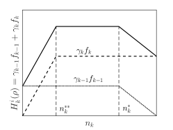
Refer to caption
Figure 8: The function Hk(n)subscript𝐻𝑘𝑛H_{k}({n}) is concave in nksubscript𝑛𝑘{n}_{k}.

Note that the intersecting points nksuperscriptsubscript𝑛𝑘{n}_{k}^{*} and nksuperscriptsubscript𝑛𝑘absent{n}_{k}^{**} of the piecewise-linear functions γk1fk1subscript𝛾𝑘1subscript𝑓𝑘1\gamma_{k-1}f_{k-1} and γkfksubscript𝛾𝑘subscript𝑓𝑘\gamma_{k}f_{k}, respectively, satisfy the following:

nksuperscriptsubscript𝑛𝑘\displaystyle{n}_{k}^{*} =nmax1w(min{βk1vnk1,βk1Fk1i}rk)absentsuperscript𝑛1𝑤subscript𝛽𝑘1𝑣subscript𝑛𝑘1subscript𝛽𝑘1superscriptsubscript𝐹𝑘1𝑖subscript𝑟𝑘\displaystyle={n}^{\max}-\frac{1}{w}(\min\{\beta_{k-1}v{n}_{k-1},\beta_{k-1}F_{k-1}^{i}\}-r_{k})
nmaxβk1Fk1iwnmaxFmaxw=ncrit,absentsuperscript𝑛subscript𝛽𝑘1superscriptsubscript𝐹𝑘1𝑖𝑤superscript𝑛superscript𝐹𝑤superscript𝑛crit\displaystyle\geq{n}^{\max}-\frac{\beta_{k-1}F_{k-1}^{i}}{w}\geq{n}^{\max}-\frac{F^{\max}}{w}={n}^{\mathrm{crit}},
nksuperscriptsubscript𝑛𝑘absent\displaystyle{n}_{k}^{**} =1βkvmin{βkFki,w(nmaxnk+1)rk+1}absent1subscript𝛽𝑘𝑣subscript𝛽𝑘superscriptsubscript𝐹𝑘𝑖𝑤superscript𝑛subscript𝑛𝑘1subscript𝑟𝑘1\displaystyle=\frac{1}{\beta_{k}v}\min\{\beta_{k}F_{k}^{i},w({n}^{\max}-{n}_{k+1})-r_{k+1}\}
FkivFmaxv=ncrit,absentsuperscriptsubscript𝐹𝑘𝑖𝑣superscript𝐹𝑣superscript𝑛crit\displaystyle\leq\frac{F_{k}^{i}}{v}\leq\frac{F^{\max}}{v}={n}^{\mathrm{crit}},

Hence, we have nknksuperscriptsubscript𝑛𝑘superscriptsubscript𝑛𝑘absent{n}_{k}^{*}\geq{n}_{k}^{**}. Thus, we conclude that Hk(n)subscript𝐻𝑘𝑛H_{k}({n}) is concave in nksubscript𝑛𝑘{n}_{k}; see Figure 8.

a.2): For k=1𝑘1k=1 and k=K𝑘𝐾k=K, the expression of Hksubscript𝐻𝑘H_{k} is simpler and thus the derivation is straightforward.

The proof of (62) is analogous.

.4 Proof of Proposition 2

We show the two conclusions in the statement separately:

(i): We can observe from (22) that F~ki(n¯,r)superscriptsubscript~𝐹𝑘𝑖¯𝑛𝑟{\widetilde{F}}_{k}^{i}(\underline{n},r) is non-increasing in n¯¯𝑛\underline{n}. Hence, for each n¯n¯superscript¯𝑛¯𝑛\underline{n}^{\prime}\leq\underline{n}, we have

F~ki(r,n¯)F~ki(n¯,r),k=1,2,,n,i.formulae-sequencesuperscriptsubscript~𝐹𝑘𝑖𝑟superscript¯𝑛superscriptsubscript~𝐹𝑘𝑖¯𝑛𝑟formulae-sequence𝑘12𝑛𝑖\displaystyle{\widetilde{F}}_{k}^{i}(r,\underline{n}^{\prime})\geq{\widetilde{F}}_{k}^{i}(\underline{n},r),\quad k=1,2,\ldots,n,\;i\in\mathcal{I}.

The conclusion follows from the above.

(ii): Consider 𝒩~𝒩~~𝒩superscript~𝒩\widetilde{\mathcal{N}}\subseteq\widetilde{\mathcal{N}}^{\prime}. Define

𝒩~1:=[ncrit,)×k=2K[n¯k,n¯k],assignsuperscriptsubscript~𝒩1superscript𝑛critsuperscriptsubscriptproduct𝑘2𝐾superscriptsubscript¯𝑛𝑘superscriptsubscript¯𝑛𝑘\displaystyle\widetilde{\mathcal{N}}_{1}^{\prime}:=\left[{n}^{\mathrm{crit}},\infty\right)\times\prod_{k=2}^{K}\left[\underline{n}_{k}^{\prime},\overline{n}_{k}^{\prime}\right],
𝒩~2:=[n¯1,ncrit]×k=2K[n¯k,n¯k].assignsuperscriptsubscript~𝒩2superscriptsubscript¯𝑛1superscript𝑛critsuperscriptsubscriptproduct𝑘2𝐾superscriptsubscript¯𝑛𝑘superscriptsubscript¯𝑛𝑘\displaystyle\widetilde{\mathcal{N}}_{2}^{\prime}:=\left[\underline{n}_{1}^{\prime},{n}^{\mathrm{crit}}\right]\times\prod_{k=2}^{K}\left[\underline{n}_{k}^{\prime},\overline{n}_{k}^{\prime}\right].

Clearly, 𝒩~1𝒩~1subscript~𝒩1superscriptsubscript~𝒩1\widetilde{\mathcal{N}}_{1}\subseteq\widetilde{\mathcal{N}}_{1}^{\prime} and 𝒩~2𝒩~2subscript~𝒩2superscriptsubscript~𝒩2\widetilde{\mathcal{N}}_{2}\subseteq\widetilde{\mathcal{N}}_{2}^{\prime}. Then, from (61) and (62), we can obtain that

i(n¯,n¯,r)=minn𝒩~1γTf(i,n,r)minn𝒩~1γTf(i,n,r)subscript𝑖¯𝑛¯𝑛𝑟subscript𝑛subscript~𝒩1superscript𝛾𝑇𝑓𝑖𝑛𝑟subscriptsuperscript𝑛superscriptsubscript~𝒩1superscript𝛾𝑇𝑓𝑖superscript𝑛𝑟\displaystyle\mathscr{F}_{i}(\underline{n},\overline{n},r)=\min_{{n}\in\widetilde{\mathcal{N}}_{1}}\gamma^{T}f(i,{n},r)\geq\min_{{n}^{\prime}\in\widetilde{\mathcal{N}}_{1}^{\prime}}\gamma^{T}f(i,{n}^{\prime},r)
=i(r,n¯,n¯),i,formulae-sequenceabsentsubscript𝑖𝑟superscript¯𝑛superscript¯𝑛for-all𝑖\displaystyle=\mathscr{F}_{i}(r,\underline{n}^{\prime},\overline{n}^{\prime}),\quad\forall i\in\mathcal{I},
i(n¯,n¯,r)=minn𝒩~2γTf(i,n,r)minn𝒩~2γTf(i,n,r)subscript𝑖¯𝑛¯𝑛𝑟subscript𝑛subscript~𝒩2superscript𝛾𝑇𝑓𝑖𝑛𝑟subscriptsuperscript𝑛superscriptsubscript~𝒩2superscript𝛾𝑇𝑓𝑖superscript𝑛𝑟\displaystyle\mathscr{F}_{i}(\underline{n},\overline{n},r)=\min_{{n}\in\widetilde{\mathcal{N}}_{2}}\gamma^{T}f(i,{n},r)\geq\min_{{n}^{\prime}\in\widetilde{\mathcal{N}}_{2}^{\prime}}\gamma^{T}f(i,{n}^{\prime},r)
=i(r,n¯,n¯),i,formulae-sequenceabsentsubscript𝑖𝑟superscript¯𝑛superscript¯𝑛for-all𝑖\displaystyle=\mathscr{F}_{i}(r,\underline{n}^{\prime},\overline{n}^{\prime}),\quad\forall i\in\mathcal{I},

The conclusion follows from the above and the fact that a1,a2,,amsubscript𝑎1subscript𝑎2subscript𝑎𝑚a_{1},a_{2},\ldots,a_{m} and b𝑏b in (31) are positive.

Acknowledgment

This work was supported by NSF Grant No. 1239054 CPS Frontiers (FORCES), MIT CEE Graduate Fellowship, and NSF CAREER Award CNS 1453126. We also sincerely appreciate the valuable inputs from the associate editor and the anonymous reviewers.

References

  • [1] Mohamed A Abdel-Aty and A Essam Radwan. Modeling traffic accident occurrence and involvement. Accident Analysis & Prevention, 32(5):633–642, 2000.
  • [2] Melike Baykal-Gürsoy, Weihua Xiao, and Kaan Ozbay. Modeling traffic flow interrupted by incidents. European Journal of Operational Research, 195(1):127–138, 2009.
  • [3] Michel Benaïm, Stéphane Le Borgne, Florent Malrieu, and Pierre-André Zitt. Qualitative properties of certain piecewise deterministic Markov processes. In Annales de l’Institut Henri Poincaré, Probabilités et Statistiques, volume 51, pages 1040–1075. Institut Henri Poincaré, 2015.
  • [4] Franco Blanchini. Survey paper: Set invariance in control. Automatica (Journal of IFAC), 35(11):1747–1767, 1999.
  • [5] El-Kébir Boukas. Stochastic Switching Systems: Analysis and Design. Springer Science & Business Media, 2007.
  • [6] Jodi Louise Carson. Best Practices in Traffic Incident Management. US Department of Transportation, Federal Highway Administration, Office of Operations, 2010.
  • [7] Bertrand Cloez, Martin Hairer, et al. Exponential ergodicity for Markov processes with random switching. Bernoulli, 21(1):505–536, 2015.
  • [8] Giacomo Como, Ketan Savla, Daron Acemoglu, Munther A Dahleh, and Emilio Frazzoli. Robust distributed routing in dynamical networks Part I: Locally responsive policies and weak resilience. Automatic Control, IEEE Transactions on, 58(2):317–332, 2013.
  • [9] Samuel Coogan and Murat Arcak. A compartmental model for traffic networks and its dynamical behavior. IEEE Transactions on Automatic Control, 60(10):2698–2703, 2015.
  • [10] Carlos F Daganzo. The cell transmission model: A dynamic representation of highway traffic consistent with the hydrodynamic theory. Transportation Research Part B: Methodological, 28(4):269–287, 1994.
  • [11] Jim G Dai and Sean P Meyn. Stability and convergence of moments for multiclass queueing networks via fluid limit models. IEEE Transactions on Automatic Control, 40(11):1889–1904, 1995.
  • [12] Mark H A Davis. Piecewise-deterministic Markov processes: A general class of non-diffusion stochastic models. Journal of the Royal Statistical Society. Series B. Methodological, 46(3):353–388, 1984.
  • [13] Gunes Dervisoglu, Gabriel Gomes, Jaimyoung Kwon, Roberto Horowitz, and Pravin Varaiya. Automatic calibration of the fundamental diagram and empirical observations on capacity. In Transportation Research Board 88th Annual Meeting, number 09-3159, 2009.
  • [14] Robert G Gallager. Stochastic Processes: Theory for Applications. Cambridge University Press, 2013.
  • [15] Gabriel Gomes, Roberto Horowitz, Alexandr A Kurzhanskiy, Pravin Varaiya, and Jaimyoung Kwon. Behavior of the cell transmission model and effectiveness of ramp metering. Transportation Research Part C: Emerging Technologies, 16(4):485–513, 2008.
  • [16] Roberto Horowitz, Adolf May, Alex Skabardonis, Pravin Varaiya, Michael Zhang, Gabriel Gomes, Laura Munoz, Xiaotian Sun, and Dengfeng Sun. Design, field implementation and evaluation of adaptive ramp metering algorithms. California Partners for Advanced Transit and Highways (PATH), 2005.
  • [17] Anxi Jia, Billy Williams, and Nagui Rouphail. Identification and calibration of site-specific stochastic freeway breakdown and queue discharge. Transportation Research Record: Journal of the Transportation Research Board, (2188):148–155, 2010.
  • [18] Li Jin and Saurabh Amin. A piecewise-deterministic Markov model of freeway accidents. In Decision and Control (CDC), 2014 IEEE 53rd Annual Conference on. IEEE, 2014.
  • [19] Li Jin and Saurabh Amin. Stability and control of piecewise-deterministic queueing systems. arXiv preprint arXiv:1604.02008, 2016.
  • [20] Li Jin and Saurabh Amin. Calibration of a macroscopic traffic flow model with stochastic saturation rates. In Transportation Research Board 96th Annual Meeting, 2017.
  • [21] Bryan Jones, Lester Janssen, and Fred Mannering. Analysis of the frequency and duration of freeway accidents in Seattle. Accident Analysis & Prevention, 23(4):239–255, 1991.
  • [22] Jeffrey P Kharoufeh and Natarajan Gautam. Deriving link travel-time distributions via stochastic speed processes. Transportation Science, 38(1):97–106, 2004.
  • [23] A Khattak, X Wang, and H Zhang. Incident management integration tool: dynamically predicting incident durations, secondary incident occurrence and incident delays. IET Intelligent Transport Systems, 6(2):204–214, 2012.
  • [24] Victor L Knoop. Road Incidents and Network Dynamics: Effects on driving behaviour and traffic congestion. PhD thesis, Technische Universiteit Delft, 2009.
  • [25] Vidyadhar G Kulkarni. Fluid models for single buffer systems. Frontiers in queueing: Models and applications in science and engineering, 321:338, 1997.
  • [26] Alexandr A Kurzhanskiy. Set-valued estimation of freeway traffic density. In Control in Transportation Systems, pages 271–277, 2009.
  • [27] Alexandr A Kurzhanskiy. Online traffic simulation service for highway incident management. Technical Report SHRP 2 L-15(C), Relteq Systems, Inc., Albany, CA, February 2013.
  • [28] Alexandr A Kurzhanskiy and Pravin Varaiya. Active traffic management on road networks: A macroscopic approach. Philosophical Transactions of the Royal Society A: Mathematical, Physical and Engineering Sciences, 368(1928):4607–4626, 2010.
  • [29] Jaimyoung Kwon, Michael Mauch, and Pravin Varaiya. Components of congestion: Delay from incidents, special events, lane closures, weather, potential ramp metering gain, and excess demand. Transportation Research Record: Journal of the Transportation Research Board, 1959(1):84–91, 2006.
  • [30] Johan Löfberg. YALMIP: A toolbox for modeling and optimization in MATLAB. In Computer Aided Control Systems Design, 2004 IEEE International Symposium on, pages 284–289. IEEE, 2004.
  • [31] Jiancheng Long, Ziyou Gao, Penina Orenstein, and Hualing Ren. Control strategies for dispersing incident-based traffic jams in two-way grid networks. IEEE Transactions on Intelligent Transportation Systems, 13(2):469–481, 2012.
  • [32] Sean P Meyn and Richard L Tweedie. Stability of Markovian processes III: Foster-Lyapunov criteria for continuous-time processes. Advances in Applied Probability, pages 518–548, 1993.
  • [33] Mahalia Miller and Chetan Gupta. Mining traffic incidents to forecast impact. In Proceedings of the ACM SIGKDD International Workshop on Urban Computing, pages 33–40, Beijing, China, August 2012. ACM.
  • [34] Nicholas Owens, April Armstrong, Paul Sullivan, Carol Mitchell, Diane Newton, Rebecca Brewster, and Todd Trego. Traffic incident management handbook. Technical report, US Department of Transportation, Federal Highway Administration, Office of Transportation Operations, 2010.
  • [35] Hyoshin Park, Ali Shafahi, and Ali Haghani. A stochastic emergency response location model considering secondary incidents on freeways. IEEE Transactions on Intelligent Transportation Systems, (99), 2016.
  • [36] David Schrank, Bill Eisele, and Tim Lomax. TTI’s 2012 urban mobility report. Proceedings of the 2012 annual urban mobility report. Texas A&M Transportation Institute, Texas, USA, 2012.
  • [37] Jiuh-Biing Sheu and Mei-Shiang Chang. Stochastic optimal-control approach to automatic incident-responsive coordinated ramp control. IEEE Transactions on intelligent transportation systems, 8(2):359–367, 2007.
  • [38] Alexander Skabardonis, Karl F Petty, Robert L Bertini, Pravin P Varaiya, Hisham Noeimi, and Daniel Rydzewski. I-880 field experiment: Analysis of incident data. Transportation Research Record: Journal of the Transportation Research Board, 1603(1):72–79, 1997.
  • [39] A Sumalee, RX Zhong, TL Pan, and WY Szeto. Stochastic cell transmission model (SCTM): A stochastic dynamic traffic model for traffic state surveillance and assignment. Transportation Research Part B: Methodological, 45(3):507–533, 2011.
  • [40] Lixian Zhang, El-Kébir Boukas, and James Lam. Analysis and synthesis of markov jump linear systems with time-varying delays and partially known transition probabilities. IEEE Transactions on Automatic Control, 53(10):2458–2464, 2008.
  • [41] RX Zhong, A Sumalee, TL Pan, and William HK Lam. Optimal and robust strategies for freeway traffic management under demand and supply uncertainties: an overview and general theory. Transportmetrica A: Transport Science, 10(10):849–877, 2014.