Adaptive Anisotropic Petrov-Galerkin Methods for First Order Transport Equations

Abstract.

This paper builds on recent developments of adaptive methods for linear transport equations based on certain stable variational formulations of Petrov-Galerkin type. The key issues can be summarized as follows. The variational formulations allow us to employ meshes with cells of arbitrary aspect ratios. We develop a refinement scheme generating highly anisotropic partitions that is inspired by shearlet systems. We establish approximation rates for $N$-term approximations from corresponding piecewise polynomials for certain compact cartoon classes of functions. In contrast to earlier results in a curvelet or shearlet context the cartoon classes are concisely defined through certain characteristic parameters and the dependence of the approximation rates on these parameters is made explicit here. The approximation rate results serve then as a benchmark for subsequent applications to adaptive Galerkin solvers for transport equations. We outline a new class of directionally adaptive, Petrov-Galerkin discretizations for such equations. In numerical experiments, the new algorithms track $C^{2}$-curved shear layers and discontinuities stably and accurately, and realize essentially optimal rates. Finally, we treat parameter dependent transport problems, which arise in kinetic models as well as in radiative transfer. In heterogeneous media these problems feature propagation of singularities along curved characteristics precluding, in particular, fast marching methods based on ray-tracing. Since now the solutions are functions of spatial variables and parameters one has to address the curse of dimensionality. We show computationally, for a model parametric transport problem in heterogeneous media in $2+1$ dimension, that sparse tensorization of the presently proposed spatial directionally adaptive scheme with hierarchic collocation in ordinate space based on a stable variational formulation high-dimensional phase space, the curse of dimensionality can be removed when approximating averaged bulk quantities.

AMS Subject Classification: Primary: 65N30,65J15, 65N12, 65N15
Key Words: Linear transport problems, $L_{2}$-stable Petrov-Galerkin formulations, $\delta$-proximality, adaptive refinements, anisotropic discretizations, best $N$-term approximation.

1. Introduction

Attempts to efficiently resolve anisotropic features in images and large data sets have triggered the development of directional representation systems like curvelets, bandlets or, more recently shearlets, see e.g. [14, 26, 27, 29, 30, 31]. These studies are motivated by the observation that “cartoon-like functions”, which are roughly speaking piecewise smooth functions with possible jump discontinuities along smooth curves (a precise definition will be given ahead), can be approximated by such systems at a better rate than those achievable by classical isotropic wavelet systems. Similarly, anisotropic meshes also allow one to obtain better approximation rates than classical shape regular meshes when the approximated functions exhibit strongly anisotropic features, see e.g. [8, 7, 6, 11]. Both concepts have been applied to images, or more generally, to (I) data directly representing the sought object, see e.g. [3, 12]. For recent advances in understanding the approximation properties of various types of (possibly discontinuous) piecewise polynomials on such meshes, ranging from hierarchies of nested meshes with and without irregular nodes to non-nested meshes obtained by local distortions, we refer e.g. to [9, 35]. In addition, piecewise polynomials on anisotropic meshes have also been used to recover (II) an implicitly given object such as the solution of an operator equation, see e.g. [6, 13]. However, in this latter context, the corresponding mesh generation is mostly heuristic in the sense that distorting or stretching a mesh is based on a given previously obtained approximation to the target function with little chance to rigorously assessing the overall accuracy or to design a refinement strategy with provable error reduction. There seem to be only very few attempts to employ directional representation systems in this context. Here one should mention the work in [5] where curvelets are used to obtain sparse approximate representations of the wave propagation operator. This is a somewhat different view of solving an operator equation than the common approaches based on adaptive discretizations. It can perhaps be better compared with computing an approximate inverse for the iterative solution of a system of equations.

The central objective of the present paper is to explore anisotropic recovery techniques in the context (II), namely for approximating solutions to operator equations which exhibit strongly anisotropic features, in such a way that the error assessment is more rigorously founded than in the presently known approaches.

Specifically, we confine the discussion to a very simple model problem, namely a linear transport equation where already discontinuities can arise, for instance, as shear layers. The reasons for this choice are the following. On one hand, linear transport is an important benchmark for stability issues. It can also be viewed as the reduced model for more complex convection-diffusion processes, highlighting the particular challenges of vanishing viscosity. Perhaps, more importantly, linear transport is the core constituent of kinetic models and Boltzmann type equations with a wide scope of applications. Therefore, we address, in particular, the treatment of parametric transport equations looking for sparse representations of the solutions as functions on a high-dimensional phase-space, i.e., the cartesian product of the spatial variables as well as of the parameters.

The layout of the paper is as follows. We briefly recall in Section 2 an adaptive refinement scheme from [17] for unsymmetric problems, specialized here to linear transport equations. It is based on a particular well conditioned variational formulation of the transport equation (in both the parametric and non-parametric case) and a strategy to realize uniformly stable Petrov-Galerkin schemes for such problems. The underlying functional analytic principles are very closely related to [2] and the so called DPG concepts, see e.g. [18, 19] as well as earlier least squares approaches [4, 32, 33]. The key feature of the present adaptive strategy is that the refinement decision hinges on the approximation of an explicitly given lifted residual in $L_{2}(D)$. This leaves considerable flexibility as to how such approximations are realized. In particular, it accommodates, in principle, classical finite element techniques with essentially no constraints on the shape of the elements, as well as directional representation systems whose frame properties are typically known in $L_{2}$.

The solutions to transport equations very much resemble the cartoon model. Depending on the right hand side, the boundary data, and the flow field, one typically encounters piecewise smooth solutions, with pieces separated by a $C^{2}$ curve. This scenario will serve as our main orientation. In Section 4.3 we develop an anisotropic approximation scheme which, on the one hand, plays well with the adaptation concept, mentioned above, and performs well in recovering cartoon like functions, viewed as a benchmark for this kind of applications. The scheme is very much inspired by recent developments centering on shearlet systems, see e.g. [26, 30]. Moreover, we derive some implications on the performance of schemes based on anisotropic bisections of partitions comprised of triangle and quadrilaterals.

In Section 5 we apply the shearlet inspired scheme to the solution of transport equations. The results quantify the predicted near-optimal performance. They also demonstrate the beneficial effect of directional adaptation to the Gibbs phenomena along jump discontinuities usually encountered.

In Section 6 we describe a numerical setup for treating parametric problems analogous to sparse tensorization of discrete ordinate methods as in [22, 23, 21], but with the directionally adaptive discretizations in physical space.

2. Model Problem - First Order Transport Equations

2.1. First Order Linear Transport Equations

We consider the domain $D\subset\mathbb{R}^{d}$, $d=2,3$, denoting as usual by $\vec{n}=\vec{n}(x)$ the unit outward normal at $x\in\partial D$. Moreover, we consider velocity fields $\vec{b}(x)$, $x\in D$, which for simplicity will always be assumed to be differentiable, i.e. $\vec{b}(x)\in C^{1}(\overline{D})^{d}$. Likewise $c(x)\in C^{0}(\overline{D})$ will serve as the reaction term in the first order transport equation

(2.1) $$A_{\circ}u:=\vec{b}\cdot\nabla u+cu =\;\mbox{$f_{\circ}$ in $D$}\,,\quad u=\;\mbox{$g$ on $\partial D_{-}$}\,,$$

where ${\partial D}_{\pm}:=\{x\in\partial D:\;\pm\vec{b}(x)\cdot\vec{n}(x)>0\}$ denotes the inflow, outflow boundary, respectively, and $f_{\circ}\in L_{2}(D)$. Furthermore, to simplify the exposition we shall always assume that

(2.2) $$c-\frac{1}{2}\nabla\cdot\vec{b}\geq c_{0}>0\quad\mbox{in}\,\,D$$

holds. In order to make use of the approximation results for shearlet inspired approximation methods in Section 4.3, we introduce a variational formulation for which the solution $u$ is a function in $L_{2}(D)$. To this end, we first multiply (2.1) by a test function and use integration by parts so that there are no derivatives applied to $u$. Following [17], one can show that the resulting bilinear form

(2.3) $$a(w,v):=\displaystyle\int_{D}\,w(-\vec{b}\cdot{\nabla}v+(c-{\nabla}\cdot\vec{b})v)\;dx,$$

is bounded on $L_{2}(D)\times W_{0}(-\vec{b},D)$, where

(2.4) $$W_{0}(\mp\vec{b},D):={\rm clos}_{\|\cdot\|_{W(\vec{b},D)}}\{v\in C^{1}(D)\cap C(\overline{D}),\,v\mid_{{\partial D}_{\pm}}\equiv 0\}.$$

and

(2.5) $$\|v\|_{W(\vec{b},D)}:=\left(\|v\|_{L_{2}(D)}^{2}+\int_{D}|\vec{b}\cdot\nabla v|^{2}\,dx\right)^{1/2}.$$

Moreover, the trace $\gamma_{-}:W_{0}(-\vec{b},D)\to L_{2}({\partial D}_{-},\omega)$ on the inflow boundary ${\partial D}_{-}$ exists and is bounded, where the latter space is endowed with the weighted $L_{2}$-norm $\|g\|^{2}_{L_{2}({\partial D}_{\pm},\omega)}=\int_{{\partial D}_{\pm}}|g|^{2}\omega ds$ with weight $\omega=|\vec{b}\cdot n|$ see, eg. [1]. Thus, the linear functional $f(\cdot)$, given by

(2.6) $$f(v):=\int_{D}f_{\circ}vdx+\int_{{\partial D}_{-}}g\gamma_{-}(v)|\vec{b}\cdot\vec{n}|ds,$$

belongs to $(W_{0}(\vec{b},D))^{\prime}$ and the variational problem

(2.7) $$a(u,v)=f(v),\quad v\in W_{0}(-\vec{b},D),$$

admits a unique solution in $L_{2}(D)$ which, when regular enough, coincides with the classical solution of (2.1), see [17, Theorem 2.2]. Taking the boundary conditions on the test functions into account, the additional boundary integral in the right hand side results from integration by parts, in analogy to the weak imposition of Neumann boundary conditions for elliptic problems.

Defining for $v\in W_{0}(-\vec{b},D)$, the adjoint $A^{*}$ of $A$ by $a(w,v)=\langle w,A^{*}v\rangle$, $(w,v)\in L_{2}(D)\times W_{0}(-\vec{b},D)$ the quantity $\|v\|_{Y}:=\|A^{*}v\|_{L_{2}(D)}$ is an equivalent norm on $W_{0}(-\vec{b},D)$. Moreover, $A:L_{2}(D)\to(W_{0}(\vec{b},D))^{\prime}$ and $A^{*}:W_{0}(\vec{b},D)\to L_{2}(D)$ are isometries (see [17, Proposition 4.1])

(2.8) $$\|A\|_{L(L_{2}(D),W_{0}(\vec{b},D)^{\prime})} =\|A^{-1}\|_{L(W_{0}(\vec{b},D)^{\prime},L_{2}(D))}=1,$$

$$\|A^{*}\|_{L(W_{0}(\vec{b},D),L_{2}(D))} =\|(A^{*})^{-1}\|_{L(L_{2}(D),W_{0}(\vec{b},D))}=1\;.$$

2.2. Parametric Transport Problems

In (2.1) $\vec{b}(x)$ is a fixed single given flow-field. Here we are also interested in the case when the convection field $\vec{b}(x,\vec{s})$ depends on a parameter that may range over some parameter set ${\mathcal{S}}$. Specifically, we now consider the parametric family of transport problems

(2.9) $$\begin{array}[]{rcl}A_{\circ}u(x,\vec{s})&=&\vec{b}(x,\vec{s})\cdot\nabla u(x,\vec{s})+c(x)u(x,\vec{s})=f(x),\;\;x\in D\subset{\mathbb{R}}^{2}\;,\\ u(x,\vec{s})&=&g(x,\vec{s})\;,\;\;x\in{\partial D}_{-}(\vec{s}),\end{array}$$

where the parameter dependent inflow-boundary ${\partial D}_{-}(\vec{s})$ is now given by

(2.10) $${\partial D}_{\pm}(\vec{s}):=\{x\in\partial D:\pm\vec{b}(x,\vec{s})\cdot\vec{n}(x)>0\},\;\;\vec{s}\in{\mathcal{S}}\;.$$

For the special case $\vec{b}(x,\vec{s})=\vec{s}$ the parametric transport problems (2.9) form a core constituent of radiative transfer models. While in the latter special case singularities of the parametric solution propagate along straight lines so that efficient directional approximation methods such as ray tracing are applicable, the present approach covers parameter dependent families of curved characteristics. Now the solution $u$ depends also on the prameter $\vec{s}$ in the convection field $\vec{b}$. Thus, for instance, when ${\mathcal{S}}=S^{2}$, the unit $2-$sphere, $u$ could be considered as a function of five variables, namely of $d=3$ spatial variables $x$ and of parameters $\vec{s}$ from the sphere ${\mathcal{S}}$. We always assume that $\vec{b}$ depends smoothly on the parameter $\vec{s}$ while for each $\vec{s}\in{\mathcal{S}}$, as a function of the spatial variable $x$, we continue to impose the same conditions as in the preceding section. The absorption coefficient $c\in L_{\infty}(D)$ will always be assumed to be nonnegative in the physical domain $D$ and to satisfy (2.2).

Following [17] we can resort to similar concepts as above to obtain a variational formulation for (2.9) over $2d-1$-dimensional phase domain $D\times{\mathcal{S}}$. To that end, let

(2.11) $$\partial D:=\partial D\times{\mathcal{S}},\quad{\partial D}_{\pm}:=\{(x,\vec{s})\in\partial D:\mp\vec{b}(x,\vec{s})\cdot\vec{n}(x)<0\},\quad{\partial D}_{0}:={\partial D}\setminus({\partial D}_{-}\cup{\partial D}_{+}),$$

and denote as before $(v,w):=(v,w)_{D\times{\mathcal{S}}}=\int_{D\times{\mathcal{S}}}v(x,\vec{s})w(x,\vec{s})dxd\vec{s}$ where, however, $d\vec{s}$ is for simplicity the normalized Haar measure on ${\mathcal{S}}$, i.e. $\int_{{\mathcal{S}}}d\vec{s}=1.$ Defining the Hilbert space

(2.12) $$W(D\times{\mathcal{S}}):=\{v\in L_{2}(D\times{\mathcal{S}}):\int_{{\mathcal{S}}\times D}|\vec{b}(\vec{s})\cdot\nabla v|^{2}dxd\vec{s}<\infty\}$$

(in the sense of distributions where the gradient $\nabla$ always refers to the $x$-variable in $D$), endowed with the norm $\|v\|_{W(D\times{\mathcal{S}})}$ given by

(2.13) $$\|v\|_{W(D\times{\mathcal{S}})}^{2}:=\|v\|_{L_{2}(D\times{\mathcal{S}})}^{2}+\int_{{\mathcal{S}}\times D}|\vec{b}(\vec{s})\cdot\nabla v|^{2}dxd\vec{s},$$

the counterpart to (2.4) is given by

(2.14) $$W^{\pm}_{0}(D\times{\mathcal{S}}):={\rm clos}_{\|\cdot\|_{W(D\times{\mathcal{S}})}}\{v\in C({\mathcal{S}},C^{1}(D)):v|_{{\partial D}_{\pm}}\equiv 0\}$$

which is again a Hilbert space under the norm $\|v\|_{W(D\times{\mathcal{S}})}$. It is shown in [17] that the problem

(2.15) $$a(u,v)=f(v)$$

with

$$a(u,v) :=\int_{D\times{\mathcal{S}}}u(-\vec{b}(\vec{s})\cdot{\nabla}v+(c-\nabla\cdot\vec{b})v)\,dx\,d\vec{s},$$

$$f(v) :=\langle f_{\circ},v\rangle+\int_{{\partial D}_{-}}g\gamma_{-}(v)|\vec{s}\cdot\vec{n}|d\vec{s},\quad v\in W^{+}_{0}(D\times{\mathcal{S}}),$$

has a unique solution in $L_{2}(D\times{\mathcal{S}})$ which, when sufficiently regular, agrees for almost every $\vec{s}\in{\mathcal{S}}$ with the corresponding classical solution of (2.9). Here $\langle f_{\circ},v\rangle$ is the dual pairing on $W^{+}_{0}(D\times{\mathcal{S}})^{\prime}\times W^{+}_{0}(D\times{\mathcal{S}})$.

3. Adaptive Scheme

Both variational formulations of Sections 2.1 and 2.2 are instances of the generic variational problem of finding $u\in X$ such that

(3.1) $$a(u,v)=\langle f,v\rangle,\quad v\in Y,$$

which is either (2.7) or (2.15). The respective spaces are $X=L_{2}(D)$ or $X=L_{2}(D\times{\mathcal{S}})$ and $Y=(W_{0}(-\vec{b},D))$ or $Y=(W^{+}_{0}(D\times{\mathcal{S}}))$.

The relevance of the isometry properties (2.8) lies in the fact that errors in $X$ are equal to the corresponding residuals in $Y^{\prime}$, i.e.,

(3.2) $$\|u-v\|_{X}=\|f-Av\|_{Y^{\prime}}\;.$$

We use this equality of errors and residuals to deal with the following two tasks:

• Devise a numerical scheme which, for a given trial space $X_{h}\subset X$, yields an approximation $u_{h}\in X_{h}$ that is near best, ie.,

  (3.3) $$\|u-u_{h}\|_{X}\leq C\inf_{w\in X_{h}}\|u-w\|_{X};$$

• Estimate errors via the residual $\|f-Au_{h}\|_{Y^{\prime}}$.

As for (I), the main idea, which also plays a central role in the recent developments of DPG schemes [18, 19], is to construct uniformly stable Petrov-Galerkin schemes. Due to (2.8), $Y_{h}:=A^{-*}X_{h}$ would be the ideal test space for a given trial space $X_{h}$, in the sense that

(3.4) $$\inf_{w\in X_{h}}\sup_{v\in Y_{h}}\frac{a(w,v)}{\|w\|_{X}\|v\|_{Y}}=1,$$

but $Y_{h}$ is practically inaccessible. One therefore settles for an approximate test space $Y_{h}$ which is sufficiently close to ideal to perserve uniform (with respect to $h$) stability. This has been quantified in [17] through the notion of $\delta$-proximality: a finite dimensional space $Z_{h}\subset Y$ is called $\delta$-proximal for $X_{h}\subset X$ for some $\delta\in(0,1)$ if the $Y$-orthogonal projection $P_{Y,Z_{h}}:Y\to Z_{h}$ satisfies

(3.5) $$\|y-P_{Y,Z_{h}}y\|_{Y}\leq\delta\|y\|_{Y},\quad y\in Y_{h}=A^{-*}X_{h}\;.$$

Note that for any $y=A^{-*}w$, $w\in X_{h}$, the projection $P_{Y,Z_{h}}y=\tilde{y}$ is given by the Galerkin projection

(3.6) $$(A^{*}\tilde{y},A^{*}z)_{X^{\prime}}=(w,A^{*}z)_{X^{\prime}},\quad v\in Z_{h},$$

and hence computable at a cost depending on ${\rm dim}\,Z_{h}$. When $Z_{h}$ is $\delta$-proximal for $X_{h}$ the test space $\tilde{Y}_{h}:=P_{Y,Z_{h}}(A^{-*}X_{h})$ turns out to give rise to uniformly stable Petrov-Galerkin schemes in a sense to be made precise in a moment. Before, we wish to point out two different ways of using this fact: in the context of discontinuous Galerkin formulations with suitably adjusted mesh-dependent norms, it is actually possible to compute a basis for $\tilde{Y}_{h}$ at a computational cost that under suitable circumstances stays essentially proportional to the dimension of $X_{h}$ [18, 19]. For conforming discretizations determining each test basis function would require solving a problem of essentially the original size. However, there is a way of realizing the Petrov-Galerkin scheme without computing the test basis functions explicitly while keeping the computational expense again essentially proportional to ${\rm dim}\,X_{h}$, [17]. To this end, using the optimal test functions in the Petrov-Galerkin scheme $a(u_{h},A^{-*}v_{h})=f(A^{-*}v_{h})$ and, using that $A^{-*}=(AA^{*})^{-1}A$, we obtain

$$\langle f-Au_{h},A^{-*}v_{h}\rangle=\langle(AA^{*})^{-1}(f-Au_{h}),Av_{h}\rangle =0 v_{h} \in X_{h},$$

where $\langle\cdot,\cdot\rangle$ is the $Y^{\prime},X$ dual pairing. Singling out $r_{h}=(AA^{*})^{-1}(f-Au_{h})$, or rather an approximation thereof, as a new variable, we obtain the saddle point problem

(3.7) $$\begin{array}[]{lcll}(A^{*}r_{h},A^{*}z_{h})_{X^{\prime}}+a(u_{h},z_{h})&=&\langle f,z_{h}\rangle,&z_{h}\in Z_{h},\\ a(v_{h},r_{h})&=&0,&v_{h}\in X_{h}.\end{array}$$

The error estimates from [17] can be summarized as follows.

Proposition 3.1.

Assume that $Z_{h}\subset Y$ is $\delta$-proximal for $X_{h}\subset X$ with some $\delta\in(0,1)$. Then the solution component $u_{h}$ of the saddle point problem (3.7) solves the Petrov-Galerkin problem

(3.8) $$a(u_{h},v)=\langle f,v\rangle,\quad v\in P_{Y,Z_{h}}(A^{-*}X_{h})\;.$$

Moreover, one has

(3.9) $$\|u-u_{h}\|_{X}\leq\frac{1}{1-\delta}\inf_{w\in X_{h}}\|u-w\|_{X},$$

and

(3.10) $$\|u-u_{h}\|_{X}+\|r_{h}\|_{Y}\leq\frac{2}{1-\delta}\inf_{w\in X_{h}}\|u-w\|_{X}.$$

Finally, one has

(3.11) $$\inf_{v_{h}\in X_{h}}\sup_{z_{h}\in Z_{h}}\frac{a(v_{h},z_{h})}{\|z_{h}\|_{Y}\|v_{h}\|_{X}}\geq{\sqrt{1-\delta^{2}}}.$$

The benefit of the above saddle point formulation is not only that it allows to bypass the computation of the test basis functions but also that provides an error estimator based on the lifted residual $r_{h}=r_{h}(u_{h},f)$ defined by (3.7). In fact, by construction $r_{h}$ is an approximation of $(AA^{*})^{-1}(f-Au_{h})$ where the additional $(AA^{*})^{-1}$ makes sure that $r_{h}$ is measured in the localizable $Y$-norm instead of the computationally generally inaccessible $Y^{\prime}$-norm of the residual. It is shown in [17] that when $Z_{h}\subset Y$ is even $\delta$-proximal for $X_{h}+A^{-1}F_{h}$ with $F_{h}\subset Y^{\prime}$ being a computationally accessible subspace, one has

(3.12) $$(1-\delta)\|f_{h}-Av_{h}\|_{Y^{\prime}}\leq\|r_{h}(v_{h},f_{h})\|_{Y}\leq\|f_{h}-Av_{h}\|_{Y^{\prime}},$$

and hence a tight bound on the residual $\|f_{h}-Av_{h}\|_{Y^{\prime}}$ obtained for the approximation $f_{h}$ of $f$. Generally, a vector $r_{h}(v_{h},f)$, which is calculated only to finite precision on a computer, cannot accurately represent every possible error for any right hand side $f$ in an infinite dimensional space but only for the prortion of $f$ that can be captured through the current discretization. Therefore the approximation $f_{h}\in F_{h}$ represents the components of $f$ visible to the error estimator. Analogously to finite element error estimators for elliptic problems, $f-f_{h}$ can be regarded as data oscillation error. Since $\|r_{h}\|_{Y}=\|A^{*}r_{h}\|_{X}$, the current error of the Petrov-Galerkin approximation $u_{h}$ is tightly estimated from below and above by the quantity $\|A^{*}r_{h}(u_{h},f_{h})\|_{X}$.

As shown in [17], the saddle point problem (3.7) is efficiently solved approximately by the Uzawa iteration

(3.13) $$\begin{array}[]{rcll}(A^{*}r^{k}_{h},A^{*}z_{h})&=&(f-Au^{k}_{h},z_{h}),&\quad z_{h}\in Z_{h},\\ (u^{k+1}_{h},v_{h})&=&(u_{h}^{k},v_{h})+(A^{*}r^{k}_{h},v_{h}),&\quad v_{h}\in X_{h}\;.\end{array}$$

The approximations $u_{h}^{k}$ to $u_{h}$ are obtained in (3.13) through simple updates while the lifted residuals $r_{h}^{k}$ result from solving a symmetric positive definite system in $Z_{h}$. See [17, Section 4.2] for more details and a proof of the following proposition.

Proposition 3.2.

Assume that $\delta$-proximality (3.5) is satisfied. Then the iterates $u_{h}^{k}$ of the Uzawa iteration converge to the solution $u_{h}$ of the saddle point problem (3.7) and

$$\|u_{h}-u_{h}^{k+1}\|_{X}\leq\delta\|u_{h}-u_{h}^{k}\|_{X}.$$

An adaptive algorithm based on the Uzawa iteration is based on the following subroutines.

ExpandStable:

For a given space $X_{h}$ return a space $Z_{h}$ such that $\delta$-proximality (3.5) is satisfied.

Approx:

For a function $w\in X$, error tolerance $\epsilon$ and a space $X_{h}$ return an approximation $w_{a}\in\hat{X}_{h}$ and a new space $\hat{X}_{h}\supset X_{h}$ such that

$$\|w-w_{a}\|_{X}\leq\epsilon\;.$$

UpdateDataSpace:

For a function $f\in Y^{\prime}$, error tolerance $\epsilon$ and spaces $F_{h}$ and $X_{h}$, return an approximation $f_{a}\in\hat{F}_{h}+AX_{h}$ and enlarged space $\hat{F}_{h}\supset F_{h}$ such that

$$\|f-f_{a}\|_{Y^{\prime}}\leq\epsilon\;.$$

According to the second row of the Uzawa iteration $u^{k+1}_{h}=u_{h}^{k}+A^{*}r_{h}^{k}$ the solution $u_{h}^{k+1}$ is updated by a residual term. Since $r_{h}^{k}\in Z_{h}$ for a stable space $Z_{h}\supset X_{h}$ and $A_{h}$ is a differential operator, we generally do not have $A^{*}r_{h}^{k}\in X_{h}$. In the standard Uzawa iteration this function is projected onto $X_{h}$. Instead, here we use the adaptive approximation Approx, giving rise to more accurate updates and better space adaptation of $X_{h}$ to approximate the solution $u$. The precise formulation of the adaptive refinement scheme is given in [17] and summarized in Algorithm 1.

Algorithm 1 Adaptive Uzawa iteration

1:Initialization: Choose a target accuracy $\epsilon$ and an initial trial space $X_{h}$. Set the initial guess, initial error bound and test space

$$u_{a} =0, errbound =\|f\|_{Y^{\prime}}, Z_{h}=\textsc{ExpandStable}(X_{h}),$$

respectively. Choose parameters $\rho,\eta,\alpha,\in(0,1)$ and $K\in\mathbb{N}$.

2:while $errbound>\epsilon$ do

3:     Compute $\hat{u}_{a}$, $\hat{r}_{a}$ as the result of $K$ Uzawa iterations with initial value $u_{a},r_{a}$ and right hand side $f_{a}$.

4:     $(update,\hat{X}_{h})=\textsc{Approx}(A^{*}\hat{r}_{a},\eta\|A^{*}\hat{r}_{a}\|_{X},X_{h})$

5:     $X_{h}:=X_{h}+\hat{X}_{h}$

6:     $(f_{a},F_{h}):=\textsc{UpdateDataSpace}(f,\alpha\rho\,errbound,F_{h},X_{h})$

7:     $Y_{h}:=\textsc{ExpandStable}(X_{h}+A^{-1}F_{h})$

8:     $u_{a}:=u_{a}+update$, $errbound:=\rho\,errbound$

9:end while

It is shown in [17, Proposition 4.7] that Algorithm 1 terminates after finitely many steps and outputs an approximate solution $u_{a}$ satisfying $\|u-u_{a}\|_{X}\leq\epsilon$. Due to the fixed error reduction per step in Proposition 3.2, a fixed number of Uzawa iterations $K$ in each loop of the algorithm is sufficient.

In the envisaged applications we either have $X=L_{2}(D)$ or $X=L_{2}(D\times{\mathcal{S}})$. Thus the actual adaptive refinement Approx is based on an $L_{2}$-approximation of an explicitly given function $A^{*}\hat{r}_{a}\in X$. This leaves some flexibility in the choice of the trial spaces $X_{h}$ and their adaptive enlargement in Approx. The approximation in $L_{2}$ is by no means constrained by any shape regularity conditions in the subdivisions of $D$ used for constructing the trial space. In particular, we are free to employ highly anisotropic approximation systems, as e.g. the shearlet inspired implementation of Approx in Section 4 below. For the actual enlargement of $X_{h}$ in Approx, one could think, for instance, of an $L_{2}$-projection $P_{X,\bar{X}_{h}}(A^{*}\hat{r}_{a})$ onto a fixed, but sufficiently large number of levels of uniform refinement $\bar{X}_{h}$ of $X_{h}$, followed by a coarsening step which, in principle, would even allow one to formulate optimality statements. As an alternative one could consider extremal problems

$$\inf_{\|A^{*}\hat{r}_{a}-w\|_{X}\leq\eta\epsilon;w\in\bar{X}_{h}}\|{\bf w}\|_{\ell_{1}},$$

where ${\bf w}$ is the coefficient vector of $w$. Moreover, in many settings an orthonormal basis of $\bar{X}_{h}$ is available so that a greedy enlargement of $X_{h}$ is efficient and yields a best $N$-term approximation of $A^{*}\hat{r}_{a}$ in $\bar{X}_{h}$.

4. Adaptive Anisotropic Approximation

The nature of solutions to linear transport equations such as (2.1) is illustrated by considering the following instances of problem (2.1).
(I): When the right hand side $f_{\circ}$ has a jump discontinuity along a smooth curve, the boundary conditions $g$ are zero, and the convection field $\vec{b}$ is $C^{1}$, the solution $u$ is only Lipschitz continuous with a jump of first order derivatives in directions not parallel to $\vec{b}$. If the discontinuity of $f_{\circ}$ is parallel to $\vec{b}$, the solution even exhibits a jump discontinuity.

(II): When $f_{\circ}$ is smooth, say constant, $\vec{b}$ is $C^{1}$, and the boundary data is piecewise smooth with a jump discontinuity, the solution will exhibit a jump discontinuity along a $C^{2}$ curve with tangents $\vec{b}$.

(III): When both, right hand side and boundary data are discontinuous both above effects superimpose.

At any rate, the solutions $u$ in the above scenarios are piecewise smooth on regions separated by a $C^{2}$ curve. In the context of image processing such functions are usually referred to as cartoon-like and serve as benchmarks for image compression schemes that are able to economically encode edges and curve-like discontinuities. In what follows we do the same in the context of solving transport equations. The methods employed in image processing cannot be directly applied in this context. One reason is the more delicate role of boundary conditions in the present context. The second one is more subtle. Since we approximate solutions in $L_{2}$ one could, in principle, employ directional representation systems such as shearlets and curvelets because they form frames in $L_{2}(\mathbb{R}^{d})$. But even setting aside the issue of boundary conditions (which would certainly destroy the tightness of such frames), one would have to determine suitable test frames whose elements are obtained by solving a global problem which renders resulting schemes inefficient. Moreover, quadrature becomes a major issue since elements of directional representation systems do not stem from nested hierarchies of multiresolution sequences. We shall therefore discuss modifications that work in the present context as well.

4.1. Isotropic Schemes

We begin recalling briefly some typical results for numerical approximations to solutions of transport equations using uniform and adaptive but isotropic meshes in both cases (I) and (II) described at the beginning of Section 4.

To this end the procedures ExpandStable and Approx need to be specified. Since $X_{h}$ is an isotropic finite element space, we can define $\textsc{ExpandStable}(X_{h})$ simply as the finite element space obtained by refining each cell of the partition of $X_{h}$ once or by increasing the polynomial degree of the finite elements.

To define $\textsc{Approx}(w,\epsilon,X_{h})$, the algorithm has to find an adaptive approximation of a known function $w$ up to prescribed accuracy $\epsilon>0$. A straightforward strategy to this end is as follows: first compute a best $L_{2}$ approximation $w_{h}\in X_{h}$ of $w$. The local errors are

$$e(T)=\|w-w_{h}\|_{L_{2}(T)}^{2}=\int_{T}|w-w_{h}|^{2}\text{d}x$$

for each cell $T$ in the partition $\mathcal{T}_{h}$ of $X_{h}$. Next, refine cells in a subset $\mathcal{S}\subset\mathcal{T}_{h}$ that are selected by a bulk criterion

$$\sum_{T\in\mathcal{S}}e(T)\geq\theta\sum_{T\in\mathcal{T}_{h}}e(T)$$

for some constant $0<\theta<1$. This is a first, rough realization for the overall algorithm and numerical experiments which are provided below. To guarantee the error bound $\epsilon>0$, we can explicitly compute the best $L_{2}(D)$ approximation $w_{ref}$ on the refined finite element space and the error $\|w-w_{ref}\|_{L_{2}}$. If the error bound $\epsilon$ is met, we stop. If it is not met, we recursively refine the finite element space again.

4.2. Benchmark Class

Let $D=(0,1)^{2}$ and assume that $\mathcal{O}$ is the class of nonempty simply connected domains $\Omega\subset\mathbb{R}^{2}$ with a $C^{2}$-boundary. Let ${\rm curv}(\partial\Omega)$ denote the curvature of $\partial\Omega\cap D$ and $|\partial\Omega\cap D|$ its length in $D$. Finally, let $C_{a}(x):=\{x^{\prime}\in\mathbb{R}^{2}:|x-x^{\prime}|<a\}$ denote the disc of radius $a$ around $x$ and define the separation width of $\Omega$

(4.1) $$\rho=\rho(\Omega):=\sup\,\{\zeta>0:\forall\,x\in\partial\Omega,\,\,\partial\Omega\cap B_{\zeta}(x)\mbox{ contains a single connected arc of }\partial\Omega\}.$$

Then, we consider the following model class of cartoon-like functions on $D=(0,1)^{2}$, defined by

(4.2) $${{\mathcal{C}}}(\kappa,L,M,\omega) := \{f_{1}\chi_{\Omega}+f_{2}\chi_{D\setminus\Omega}:\,\,\Omega\subset D,\,\Omega\in\mathcal{O},\,|\partial\Omega\cap D|\leq L,\partial\Omega\cap D\in C^{2},$$

$$\rho(\Omega)\geq\omega,\,{\rm curv}(\partial\Omega)\leq\kappa,\|f_{i}^{(l)}\|_{L_{\infty}(D)}\leq M,\,l\leq 2,\,\,i=1,2\},$$

(where the parameters $\kappa,L$ are not mutually independent). We derive approximation error bounds for anisotropic refinements for the simple scenario (4.2) making an effort to exhibit the dependence of involved constants on the class parameters $\kappa,L,M,\omega$. We shall indicate subsequently how the results extend to natural extensions of this class, e.g. admitting several components or curves with selfintersections and arbitrarily small separation width.

In the area of imaging sciences, this model has become a well accepted benchmark for sparse approximation, see, e.g., [20]. One prominent system, which does provide (near-) optimal sparse approximations for such classes are compactly supported shearlet systems for $L^{2}(\mathbb{R}^{2})$ [27, 30]. Our main point here is that, as the discussion at the beginning of this section shows, such cartoons also exhibit similar features as solutions to transport problems.

Unfortunately, even compactly supported shearlets do not comply well with quadrature and boundary adaptation tasks faced in variational methods for PDEs. We are therefore interested in generating locally refinable anisotropic partitions for which corresponding piecewise polynomial approximations realize the favorable near-optimal approximation rates for cartoon functions achieved by shearlet systems. Unfortunately, as shown in [35, Chapter 9.3], simple triangular bisections connecting the midpoint of an edge to the opposite vertex is not sufficient for warranting such rates, see [6, 7] for related work. In fact, a key feature would be to realize a “parabolic scaling law” similar to the shearlet setting, see e.g. [26]. By this we mean a sufficiently efficient directional resolution by anisotropic cells whose width scales like the square of the diameter. To achieve this we consider partitions comprising triangles and parallelograms pointed out to us in [10].

4.3. Approximation Rates

The central objective of this section is to describe and analyze a nonlinear piecewise polynomial approximation scheme on anisotropic meshes in physical space $D$ for elements from the cartoon class (4.2). Specifically, we establish approximation rates matching those obtained for shearlet systems (see [27, 30] or the survey [28]). In fact, the scheme is directly inspired by shearlet concepts in that a key element is the ability to realize the parabolic scaling law for a sufficiently rapid directional adaptation. The latter point is the main distinction of the present work from technically simpler schemes based on bisecting triangles. The envisaged error bounds, which are proved using full knowledge about the approximated function, will serve later as a benchmark for the performance of our adaptive scheme that is to approximate the unknown solution of a transport problem.

As hinted at before, we wish to analyze the approximation power of piecewise polynomial approximations based on successively constructed anisotropic meshes, utilizing the operations of parabolic scaling and shearing. The matrices associated to those two operations are defined by

(4.3) $$D_{j}=\begin{pmatrix}2^{j}&0\\ 0&2^{\lfloor j/2\rfloor}\end{pmatrix}\quad\text{and}\quad S_{k}=\begin{pmatrix}1&k\\ 0&1\end{pmatrix},\qquad j\geq 0,k\in\mathbb{Z}.$$

The relation to shearlet systems can be seen by observing that shearlets are a function system which is – except for a low frequency component – generated by application of parabolic scaling, shearing and translation operators to at least two “mother functions”. Regarding parallelograms as “prototype supports” of compactly supported shearlets we consider next partitions comprised of parallelograms and triangles only. Specifically, we set

(4.4) $$\Sigma_{N}:=\bigcup\{\mathbb{P}_{1}({\mathcal{T}}):{\mathcal{T}}\,\mbox{a partition of $D$ into parallelograms and triangles with}\,\#({\mathcal{T}})\leq N\},$$

where for any partition ${\mathcal{T}}$ of $D$ we denote by $\mathbb{P}_{1}({\mathcal{T}})$ the space of discontinuous, piecewise affine functions on the partition ${\mathcal{T}}$.

The main result shows that approximations by elements of $\Sigma_{N}$ realize (and even slightly improve on) the known rates obtained for shearlet systems for the class of cartoon-like functions [30].

Theorem 4.1.

Let $f\in{\mathcal{C}}(\kappa,M,L)$ with given cartoon $\Omega\subset D=(0,1)^{2}$, defined by (4.2). Let $\Sigma_{N}$ denote the class of all piecewise affine functions subordinate to any partition of $D$ that consists of at most $N$ cells which are either parallelograms or triangles. Then

(4.5) $$\inf_{\varphi\in\Sigma_{N}}\|f-\varphi\|_{L_{2}(D)}\leq{C(\kappa)L}\cdot M\cdot\sqrt{\log N}\cdot N^{-1},$$

where $C(\kappa)$ is an absolute constant depending only on $\kappa$.

The proof of Theorem 4.1, given in the following subsections, is based on constructing a specific sequence of admissible partitions, where the refinement decisions use full knowledge of the approximated function $f$. The above rate will then later be used as a benchmark for the performance of a fully adaptive scheme for transport equations where such knowledge about the unknown solution is, of course, not available. When repeatedly referring below to the construction in the proof of Theorem 4.1 as a “scheme” this is therefore not to be confused with the adaptive scheme presented later in Section 4.5.

4.3.1. Anisotropic Refinement Scheme

The main idea is to generate anisotropic meshes for which the cells have an approximate length $2^{-j/2}$ and width $2^{-j}$, i.e., following the parabolic scaling law “width $\approx$ length²”. This will later be seen to guarantee an improved approximation rate for the class of cartoons defined in (4.2). A very general framework for systems based on a parabolic scaling law with an analysis of such approximation rates can be found in [24], where however only unbounded domains are treated. For bounded domains $D\subset{\mathbb{R}}^{2}$ as we consider here, $L^{2}(D)$-stable systems are available in [25]. As in the previous section, given an element $f$ from the class (4.2), we shall construct now a hierarchy of specific partitions of the domain, using at this stage complete knowledge of the discontinuities of $f$.

We now describe the scheme which strongly prioritizes the generation of parallelograms. For any $J\in\mathbb{N}$ (sufficiently large depending on the parameters $\kappa,L,M$ of the cartoon class), it successively generates anisotropic meshes. For each scale $j=0,\dots,2J$, it anisotropically refines only cells intersecting the discontinuity of $f$, which will lead to about $2^{J}$ anisotropic cells whose union contains all points of discontinuity of $f$. Summing all areas of those cells gives about $2^{J}(2^{-2J}\times 2^{-J})=2^{-2J}$, which provides an $L_{2}(D)$ approximation error $\sim 2^{-J}$ for the non-smooth part of $f$. On those cells that do not intersect any discontinuity of $f$ piecewise linear approximation gives rise to an $L_{2}$ approximation error of the order of $\sim 2^{-J}$. The number of those cells turns out to be of the order of $2^{J}$ times a $\log$-factor. Combining these two error estimates, will lead to the final bound.

The refinement scheme will be based on an anisotropic refinement operator and an isotropic one, being applied in an alternating fashion. The reason is to ensure, at each scale, that the generated parallelograms follow the parabolic scaling law. Applying only the anisotropic refinement operator would, of course, lead to cells of approximate area $2^{-j}\times 1$, in violation of the parabolic scaling law.

We now proceed with studying the approximation power of our anisotropic scheme by analyzing its performance on cartoon-like functions $f\in{\mathcal{C}}(\kappa,L,M,\omega)$. Throughout this section, we denote by $P$, $Q$, ${\mathcal{C}}$ and ${\mathcal{P}}({\mathcal{C}})$, a parallelogram, a polygon (either parallelogram or triangle), a collection of cells and the power set of ${\mathcal{C}}$, respectively.

We describe the refinement scheme first for a “horizon model”, i.e., we assume

(4.6) $$\Omega=\{(x_{1},x_{2})\in D:x_{1}\leq E(x_{2})\},\quad\partial\Omega\cap D=\{(E(x_{2}),x_{2}):x_{2}\in(0,1)\},$$

where $E\in C^{2}([0,1])$ satisfies

(4.7) $$\|E^{\prime}\|_{L_{\infty}(D)}\leq 2,\quad\|E^{\prime\prime}\|_{L_{\infty}(D)}\leq\kappa.$$

Thus, $\Gamma:=\partial\Omega\cap D$ is the discontinuity curve referred to in (4.2). Accordingly, in what follows we consider for $\Omega$ from (4.6) any $f=f_{1}\chi_{\Omega}+f_{2}\chi_{D\setminus\Omega}$ with $\|f_{i}^{(l)}\|_{L_{\infty}(D)}\leq M,\,l\leq 2,\,i=1,2$, which therefore belongs to a cartoon class ${\mathcal{C}}(\kappa,M,L)$ with $L$ constrained by (4.7).

The main building blocks will be parallelograms obtained by parabolic scaling and shearing, which are defined as follows: first, choose some $J_{0}>0$ so that

(4.8) $$4\cdot 5^{3/2}\cdot\kappa\leq 2^{J_{0}}.$$

Moreover, we can choose $J_{0}$ large enough, depending on the separation parameter $\omega$, such that for every dyadic subsquare $Q\subset D$ of side-length $2^{-J_{0}}$ the curve $\Gamma$ intersects $\partial Q$ in at most two points.

The generation of an adapted partition starts with a uniform partition of $D=[0,1]^{2}$ into translates of the square $2^{-J_{0}}\cdot D$ of side length $2^{-J_{0}}$. These squares will be further subdivided as follows: for scale $j\in\mathbb{Z}$, shear $k\in\mathbb{Z}$, with corresponding operators $D_{j},S_{k}$, defined in (4.3), and position $m\in 2^{-J_{0}}D^{-1}_{j}\mathbb{Z}^{2}$, we define the parallelogram $P_{j,k,m}$ by

(4.9) $$P_{j,k,m}:=D_{j}^{-1}S_{k}(2^{-J_{0}}\cdot D)+m\;.$$

In the sequel, we refer for each fixed $j\geq 0$ to the set of all such parallelograms as ${\bf P}_{j}$, that is,

$$\mathcal{P}_{j}=\{P_{j,k,m}:k\in\mathbb{Z},m\in 2^{-J_{0}}D^{-1}_{j}\mathbb{Z}^{2}\}\;.$$

In addition to the ${\mathcal{P}}_{j}$ we consider the “trimmed” version

$$\tilde{\mathcal{P}}_{j}=\{P_{j,k,m}\cap D\cap P:P\in{\mathcal{P}}_{j-1},k\in\mathbb{Z},m\in 2^{-J_{0}}D^{-1}_{j}\mathbb{Z}^{2}\},$$

comprised of cells that are contained in $D$ as well as in parent cells from $\mathcal{P}_{j-1}$. For $\iota\in\{0,\pm 1\}$, indicating an updated shear direction, and nonnegative odd integer $j$, we introduce the following basic refinement operators: for $P=P_{j-1,k,m}$, $T_{-1}=\{(-2,0),(-1,0),(0,0)\}$, $T_{0}=\{(0,0),(1,0)\}$, and $T_{1}=\{(-1,0),(0,0),(1,0)\}$, let

(4.10) $$R^{an}_{\iota}:{\mathcal{P}}_{j-1}\rightarrow{\mathcal{P}}({\tilde{\mathcal{P}}}_{j}),\quad R^{an}_{\iota}(P)=\{P_{j,2k+\iota,m+2^{-J_{0}-j}t}\cap D\cap P:t\in T_{\iota}\}$$

which act only on parallelograms as illustrated in Figure 1.

(a)

(b)

Figure 1. Anisotropic refinements $R^{an}_{\iota}$ for $\iota=0,1$ : 1(a) $R^{an}_{0}(P_{j,k,m})$. 1(b) $R^{an}_{1}(P_{j,k,m})$.

For $j\geq 1$ we will employ next the above basic refinement operators to construct refinement operators $R_{j}$, which depend on the parity of $j$. Specifically, for positive odd integers $j$ and any parallelogram $P=P_{j-1,k,m}\in\mathcal{P}_{j-1}$, $m=(m_{1},m_{2})$, we define the orientation $\iota_{P}$ for splitting $P$ by

(4.11) $$\iota_{P}=\iota_{P}(E):=\operatornamewithlimits{argmin}_{\iota\in\{0,\pm 1\}}\Bigl{|}E^{\prime}(m_{2})-\frac{2k+\iota}{2^{\lceil j/2\rceil}}\Bigr{|}.$$

Thus, the orientation is determined by the slope of $E$ at the vertical position given by $m_{2}$. Therefore, a little care is needed when $P$ is close to the left boundary $\{(0,x_{2}):x_{2}\in[0,1]\}$ because $\Gamma$ may enter $D$ above $m_{2}$, so that $E^{\prime}(m_{2})$ is not defined. In such a case,, i.e., $|\Gamma\cap P|>0$ but $E^{\prime}(m_{2})$ is not defined, we replace $m_{2}$ by $m_{2}^{\prime}$ which is the second coordinate of the intersection of $\Gamma$ with $D$. We shall alwas assume this default choice in what follows without any formal distinction.

In addition, let $R^{iso}(Q)$ be a dyadic refinement of $Q$ into four (congruent) children of $Q$. Furthermore, define $(R^{iso})^{\ell}$ for $\ell\geq 0$ by the following recursive formula:

(4.12) $$(R^{iso})^{\ell+1}(Q)=\{Q^{\prime\prime}\in R^{iso}(Q^{\prime}):Q^{\prime}\in(R^{iso})^{\ell}(Q)\},$$

where $(R^{iso})^{0}(Q)=\{Q\}$.

Our goal is to construct next partitions of cardinality $O(N)$ with $N=2^{J}$ such that the $L_{2}$-error is of the order at most $\sqrt{J}2^{-J}$. To that end, we consider any such $J\in\mathbb{N}$ which can be thought of as significantly larger than $J_{0}$. Moreover, we define for $0\leq j\leq 2J-J_{0}$ and any cell $Q$

$$\ell_{j}^{0}(Q) :=\operatornamewithlimits{argmin}_{\ell\in\mathbb{N}_{0}}\{\exists\mbox{ rectangle $R$ of area width $\times$ height $\sim 2^{-J/2-j/4}\times 2^{-J/2+j/4}$ such that }$$

(4.13) $$\qquad(R^{iso})^{\ell^{0}_{j}(Q)}(Q)\subset R\}$$

as the smallest nonnegative integer such that each cell in $(R^{iso})^{\ell_{j}(Q)}(Q)$ is contained in a rectangle of area width $\times$ height $\sim 2^{-J/2-j/4}\times 2^{-J/2+j/4}$.

For $j=0$ the initial refinement $R_{0}(P)$ is defined as in Figure 2 and $R_{0}(P)=P$ when $\iota_{P}=0$. For $j>0$, we then define the operator $R_{j}:{\mathcal{P}}_{j-1}\to{\mathcal{P}}({\tilde{P}}_{j})$, by

(4.14) $$R_{j}(P):=\left\{\begin{array}[]{rl}R^{an}_{\iota_{P}}(P),&P\in{\mathcal{P}}_{j-1},j\mbox{ odd},\\ R^{iso}(P),&P\in{\mathcal{P}}_{j-1},j\mbox{ even},\end{array}\right.$$

We describe next the refinement procedure, which generates a sequence $\mathcal{C}_{j}$ of admissible partitions. To this end, as indicated above, we first define ${\mathcal{C}}_{0}$ by the partition of $D$ into dyadic squares of side length $2^{-J_{0}}$ as follows. Set

(4.15) $${\mathcal{C}}_{0}:=\{P_{0,0,m}:m_{1},m_{2}=0,2^{-J_{0}},\dots,1-2^{-J_{0}}\},\quad{\mathcal{C}}_{0}(\Gamma):=\{P\in{\mathcal{C}}_{0}:|P\cap\Gamma|>0\}.$$

The subsequent refinements of ${\mathcal{C}}_{0}(\Gamma)$ require one further ingredient which is the operator MERGE that reduces the number of triangles in favor of parallelograms. To explain this it is useful to introduce what we call a horizontal $\Gamma$-chain of length $l\geq 1$

$$\mathcal{H}_{j,m_{2}}(\Gamma):=\left\{P_{j,k,(m_{1,i},m_{2})}:\mbox{for some k, }\begin{array}[]{l}|P_{j,k,(m_{1}+i-1,m_{2})}\cap\Gamma|>0,i=1,\ldots,l,\\ |P_{j,k,(m_{1}-1,m_{2})}\cap\Gamma|=|P_{j,k,(m_{1}+l,m_{2})}\cap\Gamma|=0\end{array}\right\}$$

comprised of a maximal collection of parallelograms at a fixed vertical level $m_{2}$ which have the same orientation and intersect $\Gamma$ substantially. In particular, we can decompose ${\mathcal{C}}_{0}(\Gamma)=\bigcup_{m_{2}}\mathcal{H}_{0,m_{2}}(\Gamma)$.

Defining for any collection of parallelograms ${\mathcal{C}}$

$$R_{j}({\mathcal{C}}):=\{R_{j}(P):P\in{\mathcal{C}}\},$$

in particular, when $j$ is odd the collection $R_{j}\big{(}\mathcal{H}_{j,m_{2}}(\Gamma)\big{)}$ contains in general parallelograms and triangles. We make essential use of the following observation.

Lemma 4.2.

Assume that $j$ is even and $\mathcal{H}_{j,m_{2}}(\Gamma)$ is a horizontal $\Gamma$-chain of length $l$ none of whose elements intersects the left or right vertical part of $\partial D$. Then, replacing all pairs of contiguous triangles in $R_{j+1}\big{(}\mathcal{H}_{j,m_{2}}(\Gamma)\big{)}$ whose union is a parallelogram by this parallelogram while keeping all other cells in $R_{j+1}\big{(}\mathcal{H}_{j,m_{2}}(\Gamma)\big{)}$ the same, yields a collection

$$\mbox{\rm MERGE}\big{(}\mathcal{H}_{j,m_{2}}(\Gamma)\big{)}$$

with the following properties: all cells $Q$ in $\mbox{\rm MERGE}\big{(}\mathcal{H}_{j,m_{2}}(\Gamma)\big{)}$ that substantially intersect $\Gamma$, i.e., $|Q\cap\Gamma|>0$, form a horizontal $\Gamma$-chain of length not larger than $2l-1$.

Proof.

The validity of the above claim is easily confirmed by noting that by (4.11) $\iota_{P}=\iota_{P^{\prime}}$ for any two $P,P^{\prime}\in\mathcal{H}_{j,m_{2}}$ and using the maximality of a horizontal $\Gamma$-chain.  

For arbitrary, finite union $\mathcal{H}$ of horizontal $\Gamma$-chains we denote

$$\mbox{MERGE}\big{(}\mathcal{H}\big{)}:=\bigcup\,\big{\{}\mbox{MERGE}\big{(}\mathcal{H}_{j,m_{2}}(\Gamma)\big{)}:\mathcal{H}_{j,m_{2}}(\Gamma)\in\mathcal{H}\big{\}}.$$

The statement in Lemma 4.2 regarding the fact that $\Gamma$ is only intersected by parallelograms after merging, is not necessarily true when the first or last parallelogram $P$ in a horizontal $\Gamma$-chain intersects the left or right vertical boundary part of $D$, respectively. In fact, when $\iota_{P}\neq 0$ the left and rightmost triangles cannot be merged but may still be substantially intersected by $\Gamma$. To account for this fact, note first that due to the constraints on $\Gamma$ there exist at most a finite number of intersections of $\Gamma$ with vertical boundary portions of $\partial D$. We may assume without loss of generality that $J_{0}$ is large enough (depending only on the parameters $\kappa,L,\omega$) such that a cell in ${\mathcal{C}}_{0}$ contains at most one intersection of $\Gamma$ with the vertical boundary

$$(\partial D)^{v}:=\{(\bar{x},x_{2}):\bar{x}\in\{0,1\},\,x_{2}\in[0,1]\}.$$

Let us denote

(4.16) $${\mathcal{C}}_{0}^{B}:=\{P\in{\mathcal{C}}_{0}:P\cap\Gamma\cap(\partial D)^{v}\neq\emptyset\},\quad{\mathcal{C}}_{0}^{\prime}(\Gamma):={\mathcal{C}}_{0}(\Gamma)\setminus{\mathcal{C}}_{0}^{B}.$$

As said before $\#({\mathcal{C}}_{0}^{B})$ is finite depending only on $\kappa,L,\omega$.

We are now prepared to describe the refinement process first only for the cells in ${\mathcal{C}}_{0}^{\prime}(\Gamma)$, ${\mathcal{C}}_{0}^{\prime}:={\mathcal{C}}_{0}\setminus{\mathcal{C}}_{0}^{B}$. As mentioned before ${\mathcal{C}}^{\prime}_{0}(\Gamma)$ can be decomposed into horizontal $\Gamma$-chains so that the collection

(4.17) $${\mathcal{C}}^{an}_{0,0}=\mbox{MERGE}(\{Q\in R_{0}(P):P\in{\mathcal{C}}^{\prime}_{0}(\Gamma)\})=\mbox{MERGE}\big{(}R_{1}({\mathcal{C}}^{\prime}_{0}(\Gamma))\big{)}$$

is well defined and has, by Lemma 4.2, the following property: all cells $Q$ in ${\mathcal{C}}^{an}_{0,0}$ that substantially intersect $\Gamma$ are parallelograms with the same shear orientation for each vertical level.

Given ${\mathcal{C}}^{an}_{0,0}$, we can initialize the collection

(4.18) $${\mathcal{C}}^{iso}_{0,0}:=\{Q^{\prime}\in(R^{iso})^{\ell^{0}_{0}(Q)}(Q):Q\in{\mathcal{C}}^{an}_{0,0}\cup{\mathcal{C}}^{\prime}_{0},|Q\cap\Gamma|=0\}$$

of those cells that result from an isotropic refinement of the cells $Q$ with $|Q\cap\Gamma|=0$, see Figure 3 and the definition (4.3.1) of the refinement depth $\ell^{0}_{0}(Q)$.

On account of Lemma 4.2, we can now recursively define $({\mathcal{C}}_{j}^{an})_{j,0}$ and $({\mathcal{C}}_{j}^{iso})_{j,0}$, $j>0$ by

(4.19) $${{\mathcal{C}}}^{an}_{j,0}:=\mbox{MERGE}(\{Q^{\prime}\in{{R}_{j}(Q)}:Q\in{\mathcal{C}}^{an}_{j-1,0},|Q\cap\Gamma|\neq 0\}),\quad 0<j\leq 2J-J_{0},$$

and

(4.20) $${\mathcal{C}}^{iso}_{j,0}:=\{Q^{\prime}\in(R^{iso})^{\ell^{0}_{j}(Q)}(Q):Q\in{\mathcal{C}}^{an}_{j,0},|Q\cap\Gamma|=0\},$$

see (4.3.1) for the definition of $\ell^{0}_{j}(Q)$ as the smallest integer for which each cell in $(R^{iso})^{\ell^{0}_{j}(Q)}(Q)$ is contained in a rectangle of area width $\times$ height $\sim 2^{-J/2-j/4}\times 2^{-J/2+j/4}$. We also set ${{\mathcal{C}}}^{an}_{j,0}:=\emptyset$ for $j>2J-J_{0}$.

(a)

(b)

Figure 2. Initial refinement $R_{0}(P)$ : 2(a) $R_{0}(P)$ for $P\in{\mathcal{P}}_{0}$ when $\iota_{P}=1$. 2(b) $R_{0}(P)$ for $P\in{\mathcal{P}}_{0}$ when $\iota_{P}=-1$.

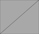
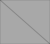
Note that the collections ${\mathcal{C}}^{an}_{j,0},{\mathcal{C}}^{iso}_{j,0}$ give rise to partitions. Since the initializing collections contain only pairwise disjoint cells it is clear that the collections ${\mathcal{C}}_{j,0}^{an}$ and ${\mathcal{C}}_{j,0}^{iso}$ are also only comprised of cells with pairwise disjoint interiors. More precisely, for any $m\in\mathbb{N}$, the collection

(4.21) $${\mathcal{C}}_{m,0}(f):={\mathcal{C}}^{an}_{m,0}\cup\bigcup_{j<m}{\mathcal{C}}^{iso}_{j,0}$$

forms a partition of

$$D_{0}:=[0,1]^{2}\setminus\bigcup\,\{P\in{\mathcal{C}}_{0}^{B}\}$$

comprised of parallelograms and triangles.

Figure 3. Recursive construction of ${\mathcal{C}}^{an}_{j}$ and ${\mathcal{C}}^{iso}_{j}$.

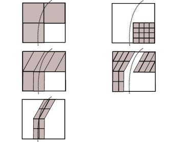
It remains to construct similar partitions for the remaining squares $P_{0}\in{\mathcal{C}}_{0}^{B}$ with nonempty intersection with $(\partial D)^{v}$. There is a uniform upper bound $B$ of such cells over the given cartoon class, depending only on the parameters $\kappa,L,\omega$. Thus it suffices to discuss one such square $P_{0}$ of side length $2^{-J_{0}}$ in ${\mathcal{C}}_{0}^{B}$ whose vertical boundary has exactly one point $g$ of intersection with $\Gamma$. Hence, there exists exactly one square $P_{1}\in R^{iso}(P_{0})$ that contains $g$. Let

$${\mathcal{C}}^{\prime}_{0,1}:=R^{iso}(P_{0})\setminus\{P_{1}\},\quad{\mathcal{C}}^{\prime}_{0,1}(\Gamma):=\{P^{\prime}\in{\mathcal{C}}^{\prime}_{0,1}:|P^{\prime}\cap\Gamma|>0\}.$$

More generally, for $r\in\mathbb{N}_{0}$, let $P_{r}(P_{0})\subset P_{0}$ be the unique square of side length $2^{-J_{0}-r}$ containing the intersection point $g$ and define

(4.22) $${\mathcal{C}}^{\prime}_{0,r+1}:=R^{iso}(P_{r})\setminus\{P_{r+1}\},\quad{\mathcal{C}}^{\prime}_{0,r+1}(\Gamma):=\{P^{\prime}\in{\mathcal{C}}^{\prime}_{0,r+1}:|P^{\prime}\cap\Gamma|>0\}.$$

For each collection ${\mathcal{C}}^{\prime}_{0,r}$, $0\leq r\leq J-J_{0}$, we can now apply the above construction to arrive at collections ${\mathcal{C}}^{an}_{j,r},{\mathcal{C}}^{iso}_{j,r}$, $j>0$, providing partitions

(4.23) $${\mathcal{C}}^{\prime}_{m,r}(f,P_{0}):={\mathcal{C}}^{an}_{m,r}\cup\bigcup_{j<m}{\mathcal{C}}^{iso}_{j,r}$$

of the $L$-shaped domains

$$D_{r}=D_{r}(P_{0}):=P_{r}\setminus P_{r+1}\subset P_{0}.$$

Note that it suffices to stop this zoom as soon as $P_{r+1}$ has side length $2^{-J}$ because when approximating $f$ on $P_{r+1}$ by zero, the squared $L_{2}$-error on this square is bounded by $M^{2}$ times its area which is $2^{-2J}$ and there are at most $\#({\mathcal{C}}_{0}^{B})$ such squares each contributing a squared error of the order $2^{-2J}$ which is within our target accuracy, i.e., $0\leq r\leq J-J_{0}-1$. For each $r$ in this range we need to consider only anisotropic refinements of level up to $2J$ which yields the following ranges

(4.24) $$0\leq j\leq 2J-J_{r},\quad 0\leq r\leq J-J_{0}-1,\quad\mbox{where}\quad J_{r}:=J_{0}+r.$$

Thus, on each $P_{0}\in{\mathcal{C}}_{0}^{B}$ we are led to consider the partition

(4.25) $${\mathcal{T}}_{J}(P_{0}):=\{P_{J-J_{0}}\}\cup\bigcup_{r=0}^{J-J_{0}-1}{\mathcal{C}}^{\prime}_{J+1,r}(f,P_{0})$$

of $P_{0}$ so that

(4.26) $${\mathcal{T}}_{J}(f):={\mathcal{C}}_{2J-J_{0},0}(f)\bigcup_{P_{0}\in{\mathcal{C}}_{0}^{B}}{\mathcal{T}}_{J}(P_{0})$$

is a partition of $D$ adapted to $f$, see (4.21).

4.3.2. Proof of Theorem 4.1

We are now ready to provide the proof of Theorem 4.1 by analyzing the approximation error provided by ${\mathcal{T}}_{J}(f)$ first under the above restricted assumptions on $f\in{\mathcal{C}}(\kappa,L,M,\omega)$. Once such a result is at hand, we point out how to extend it to the full cartoon class.

We adhere to the notation of the preceding section and denote for any partition ${\mathcal{T}}$ by $\mathbb{P}_{p}({\mathcal{T}})$ the space of piecewise polynomials of degree at most $p\in\mathbb{N}$ subordinate to the partition ${\mathcal{T}}$.

Recalling the definition (4.4) of $\Sigma_{N}$, we determine for given cartoon $f$ in ${\mathcal{C}}(\kappa,L,M,\omega)$ the cardinality $N=N(J):=\sharp({\mathcal{T}}_{J}(f))$, for ${\mathcal{T}}_{J}(f)$ defined by (4.26), and then estimate $\inf_{g\in\mathbb{P}_{1}({\mathcal{T}}_{J}(f))}\|f-g\|_{L_{2}(D)}$.

By construction, we have $\mathbb{P}_{1}({\mathcal{T}}_{m}(f))\subset\Sigma_{\#({\mathcal{T}}_{m}(f))}$. We assume first that the discontinuity curve $\Gamma=\partial\Omega\cap D$ is given as in (4.6). Moreover, we analyze first the approximation from the spaces $\mathbb{P}_{1}({\mathcal{C}}_{m,0}(f))$ on the domain $D_{0}$ (excluding the squares with vertical boundary intersections of $\Gamma$), see (4.21). To simplify notation we abbreviate in this part of the proof

$${\mathcal{C}}^{an}_{j}:={\mathcal{C}}^{an}_{j,0},\quad{\mathcal{C}}^{iso}_{j}:={\mathcal{C}}^{iso}_{j,0},\quad\ell_{j}(Q):=\ell_{j}^{0}(Q).$$

We begin with recording the following properties of the collections ${\mathcal{C}}^{an}_{j}$ that will be used repeatedly:

• $\Bigl{|}\Gamma\cap\Bigl{(}\bigcup_{Q\in\mathcal{C}^{an}_{j}}Q\Bigl{)}^{c}\Bigr{|}=0$.

• For each $Q\in\mathcal{C}^{an}_{j}$ with $|Q\cap\Gamma|>0$, we have $Q=P\subset D$ for some $P=P_{j,k,m}$ and

  (4.27) $$\sup_{(x_{1},x_{2})\in Q}\Bigl{|}E^{\prime}(x_{2})-\frac{k}{2^{\lceil j/2\rceil}}\Bigr{|}\leq\frac{1}{2^{\lceil j/2\rceil}}.$$

• In (C2), $P$ is a parallelogram of size width $\times$ height $\lesssim 2^{-j}\times 2^{-j/2}$.

We now verify first the validity of these properties. (C1) and (C3) follow directly from our construction. We verify next (C2) by induction on $j$. For $j=0$ note first that for $m_{2}\leq s\leq m_{2}+2^{-J_{0}}$

(4.28) $$|E^{\prime}(s)-E^{\prime}(m_{2})|\leq\int_{m_{2}}^{s}|E^{\prime\prime}(t)|dt\leq(4\cdot 5^{3/2})^{-1},$$

where we have used (4.8). Let us consider first $E^{\prime}(m_{2})\geq 0$. Then we have $\iota_{P}=0$, if $E^{\prime}(m_{2})<1/2$, and $\iota_{P}=1$ when $E^{\prime}(m_{2})\geq 1/2$. When $E^{\prime}(s)$ remains positive we have $|E^{\prime}(s)-1|\leq 1$, by (4.7), which confirms the claim in this case. When $E^{\prime}(s)<0$ for some $s$ (4.28) says that $|E^{\prime}(s)-E^{\prime}(m_{2})|=|E^{\prime}(m_{2})|+|E^{\prime}(s)|\leq(4\cdot 5^{3/2})^{-1}$ which gives $\iota_{P}=0$ and again confirms the claim for $j=0$. An analogous argument can be used when $E^{\prime}(m_{2})<0$ to conclude that (4.27) holds for $j=0$.

Let us assume now that $j\geq 0$ is even and that (4.27) is satisfied for this $j$. We then prove that

(4.29) $$\sup_{(x_{1},x_{2})\in Q^{\prime}}\Bigl{|}E^{\prime}(x_{2})-\frac{2k+\hat{\iota}}{2^{\lceil(j+1)/2\rceil}}\Bigr{|}\leq\frac{1}{2^{\lceil(j+1)/2\rceil}}$$

for any $Q^{\prime}\in R^{an}_{\hat{\iota}}(P_{j,k,m})$ with $|Q^{\prime}\cap\Gamma|\neq 0$, where

(4.30) $$\hat{\iota}=\operatornamewithlimits{argmin}_{\iota\in\{0,\pm 1\}}\Bigl{|}E^{\prime}(m_{2})-\frac{2k+\iota}{2^{j/2+1}}\Bigr{|}.$$

By Lemma 4.2 and because we are working only on $D_{0}$, we can assume without loss of generality that $Q^{\prime}=P_{j+1,2k+\hat{\iota},\tilde{m}}\in{\bf P}_{j+1}$ with $\tilde{m}=(\tilde{m}_{1},m_{2})$, for some $\tilde{m}_{1}\in(0,1)$, is a parallelogram contained in $D$. If $(x_{1},x_{2})\in P_{j+1,2k+\hat{\iota},\tilde{m}}$, then

(4.31) $$|x_{2}-m_{2}|\leq 2^{-J_{0}-j/2}$$

Thus

$$\Bigl{|}E^{\prime}(x_{2})-\frac{2k+\hat{\iota}}{2^{j/2+1}}\Bigr{|}\leq\Bigl{|}E^{\prime}(m_{2})-\frac{2k+\hat{\iota}}{2^{j/2+1}}\Bigr{|}+|E^{\prime}(m_{2})-E^{\prime}(x_{2})|.$$

This now implies that

$$\sup_{Q^{\prime}\in(x_{1},x_{2})}\Bigl{|}E^{\prime}(x_{2})-\frac{2k+\hat{\iota}}{2^{\lceil(j+1)/2\rceil}}\Bigr{|}\leq\Bigl{|}E^{\prime}(m_{2})-\frac{2k+\hat{\iota}}{2^{j/2+1}}\Bigr{|}+|E^{\prime}(m_{2})-E^{\prime}(x_{2})|=\text{(I)}+\text{(II)}.$$

By (4.27) and (4.30),

$$\text{(I)}\leq(\frac{1}{2})2^{-j/2-1}.$$

Again, by (4.31),

$$\text{(II)}\leq\|E^{\prime\prime}\|_{\infty}2^{-J_{0}-j/2}\leq(\frac{1}{2})2^{-j/2-1},$$

where in the last step we have used the condition (4.8) on the initial scale $J_{0}$. This proves (4.29).

Finally, when $j$ is odd, we note that (4.27) obviously implies (4.29) for any $Q^{\prime}\in R^{iso}(P_{j,k,m})$, since $\lceil j/2\rceil=\lceil(j+1)/2\rceil$. Thus, (C2) follows by induction.

We proceed bounding next $\#({\mathcal{C}}_{2J{-J_{0}}}(f))$, see (4.21), and noting that ${\rm dim}\,(\mathbb{P}_{1}({\mathcal{C}}_{2J{-J_{0}}}(f)))=3\#({\mathcal{C}}_{2J{-J_{0}}}(f))$. To this end, (C2) and (C3) together with the fact that each $P\in{\mathcal{C}}^{an}_{j}$ is for $j>0$ a refinement of some $P^{\prime}\in{\mathcal{C}}^{an}_{j-1}$ intersecting $\Gamma$, the length of $\Gamma\cap Q$ scales for $Q\in{\mathcal{C}}_{j}^{an}$ asymptotically like ${\rm diam}\,(Q)\sim 2^{-J_{0}-j/2}$ so that

(4.32) $$\sharp(\mathcal{C}^{an}_{j})\lesssim L2^{J_{0}+j/2},\quad j\geq 0,$$

with a constant depending only on $\kappa$. Hence, we obtain

(4.33) $$\sharp\Bigl{(}\bigcup_{j=0}^{2J{-J_{0}}}{\mathcal{C}}^{an}_{j}\Bigr{)}\lesssim{L2^{J_{0}}}\sum_{j=0}^{2J{-J_{0}}}2^{j/2}\lesssim L2^{J{+J_{0}/2}},$$

with a constant depending only on $\kappa$. Note that our count is generous because of the overlap of cells on different levels $j$. By majorization with a summable geometric series, such redundancies are always controlled by a constant uniform factor.

We now estimate $\sharp(\bigcup_{j=0}^{2J}{\mathcal{C}}^{iso}_{j})$ observing first that for each $Q\in{\mathcal{C}}^{an}_{j}$,

$$\sharp((R^{iso})^{\ell_{j}(Q)}(Q))=2^{2\ell_{j}(Q)},$$

where $\ell_{j}(Q)=\ell_{j}^{0}(Q)$ (as defined in (4.3.1)) is chosen so that $2^{-\ell_{j}(Q)}Q$ is contained in a rectangle of size width $\times$ height $\lesssim 2^{-\frac{J}{2}-\frac{j}{4}}\times 2^{-\frac{J}{2}+\frac{j}{4}}$. This is accomplished by taking

(4.34) $$\ell_{j}(Q)=\ell_{j}^{0}(Q)=\max\,\Big{\{}\Big{\lceil}\frac{J}{2}-\frac{3j}{4}-J_{0}\Big{\rceil},0\Big{\}},$$

i.e., $\ell_{j}(Q)=0$ when $j\geq 2(J-2J_{0})/3$. Therefore, by (4.20), we obtain, upon recalling that $\sharp({\mathcal{C}}^{an}_{j})\lesssim L2^{{J_{0}+}j/2}$

(4.35) $$\sharp(\bigcup_{j=0}^{2J{-J_{0}}}{\mathcal{C}}^{iso}_{j}) {\leq} \sum_{j=0}^{\lceil\frac{2J}{3}{-\frac{4J_{0}}{3}}\rceil}2^{2(J/2-3/4j{-J_{0}})}\sharp({\mathcal{C}}^{an}_{j})+\sum_{j>\lceil\frac{2J}{3}{-\frac{4J_{0}}{3}}\rceil}\sharp({\mathcal{C}}^{an}_{j})$$

$$\lesssim L\Big{(}\sum_{j=0}^{\lceil\frac{2J}{3}{-\frac{4J_{0}}{3}}\rceil}{2^{J-j-J_{0}}}+{2^{J_{0}}}\sum_{j=\lceil\frac{2J}{3}{-\frac{4J_{0}}{3}}\rceil+1}^{2J{-J_{0}}}2^{j/2}\Big{)}\lesssim L2^{J{+J_{0}/2}},$$

where we have used (4.33) in the last step, so that the constant in the above estimate depends only on $\kappa$.

In summary, by (4.33) and (4.35), we conclude that

(4.36) $$N={\rm dim}\,\mathbb{P}_{1}({\mathcal{C}}_{2J{-J_{0}},0}(f))\lesssim{L{2^{J_{0}/2}}2^{J}=:{2^{J_{0}/2}}L\,N_{0},\quad N_{0}\sim 2^{J}},$$

see (4.21), with a constant depending only on $\kappa$ and $\omega$.

After bounding the number of degrees of freedom associated with the constructed partition we now turn to estimating the approximation error. To this end, recall that, by (4.21), ${\mathcal{C}}_{2J{-J_{0}}}(f)={\mathcal{C}}^{an}_{2J{-J_{0}}}\cup{\mathcal{C}}^{iso}$, where ${\mathcal{C}}^{iso}=\cup_{j=0}^{2J-1{-J_{0}}}{\mathcal{C}}^{iso}_{j}$ and notice further that on account of (C1), (4.19), (4.20), one has $|Q\cap\Gamma|=0$ for any $Q\in{\mathcal{C}}^{iso}$. Thus, for $Q\in{\mathcal{C}}^{iso}$, denoting by $P_{Q}(f)$ the best $L_{\infty}$-approximation to $f$ from $\mathbb{P}_{1}$ on $Q$, a classical Whitney estimate states $\|f-P_{Q}(f)\|_{L_{\infty}(Q)}\leq C({\rm diam}\,(Q))^{2}\|f\|_{{W^{2,\infty}(Q)}}$ where $C>0$ is independent of the aspect ratio of $Q$. Thus, since $f\in{\mathcal{C}}(\kappa,L,M,\omega)$, we conclude that

(4.37) $$\|f-P_{Q}(f)\|^{2}_{L_{2}(Q)}\leq|Q|\|f-P_{Q}(f)\|_{L_{\infty}(Q)}^{2}{\leq C({\rm diam}\,(Q))^{4}|Q|M^{2}}\;.$$

If $Q\in{\mathcal{C}}^{iso}_{j}$ with $j>\lfloor\frac{2J}{3}{-\frac{4J_{0}}{3}}\rfloor$, then $|Q|\lesssim 2^{-j{-J_{0}}}\times 2^{-j/2{-J_{0}}}$ and ${\rm diam}\,(Q)\lesssim 2^{-j/2{-J_{0}}}$, so that, by (4.37),

(4.38) $$\|f-P_{Q}(f)\|^{2}_{L_{2}(Q)}\lesssim 2^{-\frac{7}{2}j}{2^{-6J_{0}}}M^{2}\;.$$

On the other hand, if $Q\in{\mathcal{C}}^{iso}_{j}$ with $j\leq\lfloor\frac{2J}{3}{-\frac{4J_{0}}{3}}\rfloor$, then $|Q|\lesssim 2^{-j-\ell_{j}(Q){-J_{0}}}\times 2^{-j/2-\ell_{j}(Q){-J_{0}}}$, ${\rm diam}\,(Q)\sim 2^{\frac{j}{4}-\frac{J}{2}}$ with $\ell_{j}(Q){\sim}\lceil J/2-3j/4{-J_{0}}\rceil$ and the same reasoning yields

(4.39) $$\|f-P_{Q}(f)\|^{2}_{L_{2}(Q)}\lesssim 2^{j-3J}M^{2}\;.$$

Therefore, the approximation error away from $\Gamma$ can be bounded by

(4.40) $$\sum_{Q\in{\mathcal{C}}^{iso}}\|f-P_{Q}(f)\|^{2}_{L_{2}(Q)} \lesssim \sum_{j=\lceil\frac{2J}{3}{-\frac{4J_{0}}{3}}\rceil+1}^{2J-1{-J_{0}}}\sum_{Q\in{{\mathcal{C}}}^{iso}_{j}}\|f-P_{Q}(f)\|^{2}_{L_{2}(Q)}$$

$$\quad+\sum_{j=0}^{\lceil\frac{2J}{3}{-\frac{4J_{0}}{3}}\rceil}\sum_{Q\in\mathcal{C}^{iso}_{j}}\|f-P_{Q}(f)\|^{2}_{L_{2}(Q)}$$

$$\lesssim LM^{2}\Big{(}{2^{-7J_{0}}2^{J}}\sum_{j=\lceil\frac{2J}{3}{-\frac{4J_{0}}{3}}\rceil}^{2J-1{-J_{0}}}{2^{-\frac{9j}{2}}}+\sum_{j=0}^{\lceil\frac{2J}{3}{-\frac{4J_{0}}{3}}\rceil}{2^{J-j-J_{0}}2^{j-3J}}\Big{)}$$

$$\lesssim {2^{-J_{0}}}LM^{2}2^{-2J}{\Big{(}1+\left\lceil\frac{2J}{3}{-\frac{4J_{0}}{3}}\right\rceil_{+}\Big{)}}$$

$$\sim L\,M^{2}{2^{-J_{0}}}(\log N_{0})N_{0}^{-2},$$

where the constant depends only on $\kappa$ and $\left\lceil\frac{2J}{3}{-\frac{4J_{0}}{3}}\right\rceil_{+}:=\max\left\{0,\left\lceil\frac{2J}{3}{-\frac{4J_{0}}{3}}\right\rceil\right\}$.

It remains to bound the error on the cells in ${\mathcal{C}}^{an}_{2J{-J_{0}}}$. Due to the jump of $f$ across $\Gamma$ we simply take $0$ as an approximation to $f$ on the cells in ${\mathcal{C}}^{an}_{2J{-J_{0}}}$. Thus, we obtain

(4.41) $$\sum_{Q\in{\mathcal{C}}^{an}_{2J{-J_{0}}}}\|f\|^{2}_{L_{2}(Q)}\lesssim\sharp({\mathcal{C}}^{an}_{2J{-J_{0}}})2^{-3J{-J_{0}/2}}{M^{2}}\lesssim(2^{-2J}){L\,M^{2}},$$

with a constant depending only on $\kappa$. Therefore, adding (4.40) and (4.41), we obtain

(4.42) $$\inf_{\varphi\in\Sigma_{N}}\|f-\varphi\|_{L_{2}(D_{0})}^{2}\lesssim L\,M^{2}(\log N_{0})N_{0}^{-2},$$

with a constant depending only on $\kappa$. This proves our claim for discontinuity curves exhibiting the special form (4.6) under the constraints in (4.7) on the restricted domain $D_{0}$.

We treat next the remaining cells in ${\mathcal{C}}_{0}^{B}$. Since there is a uniform finite bound on the number of these squares, depending only on $\kappa,L$, it suffices to analyze the complexitity of the partitions ${\mathcal{C}}^{\prime}_{j,r}(f,P_{0})$ where $P_{0}\in{\mathcal{C}}_{0}^{B}$. Recall that ${\mathcal{C}}^{\prime}_{0,r}$ is the initial partition of an $L$-shaped domain consisting of $3$ squares of side length $2^{-J_{r}}$ where we abbreviate for convenience $J_{r}:=J_{0}+r$. We can estimate the cardinalities of the corresponding partitions ${\mathcal{C}}_{j,r}^{an},{\mathcal{C}}_{j,r}^{iso}$ along the same lines as before, taking the respective scalings into account. First we note that

(4.43) $$\sharp({\mathcal{C}}^{an}_{j,r})\lesssim L2^{j/2},\quad j\geq 0.$$

Since the highest refinement level should not exceed $2J$ we obtain

(4.44) $$\sharp\Big{(}\bigcup_{j=0}^{2J-J_{r}}{\mathcal{C}}^{an}_{j,r}\Big{)}\lesssim L\sum_{j=0}^{2J-J_{r}}2^{j/2}\lesssim L2^{J-J_{r}/2}.$$

The analogous isotropic refinement depth $\ell^{r}_{j}(Q)$ for $Q\in{\mathcal{C}}^{an}_{j,r}$ not intersecting $\Gamma$, that ensures that $(R^{iso})^{\ell^{r}_{j}(Q)}(Q)$ fits into a rectangle of width $\sim 2^{-\frac{J}{2}-\frac{j}{4}}$ and length $\sim 2^{-\frac{J}{2}+\frac{j}{4}}$, takes now the form

(4.45) $$\ell_{j}^{r}(Q)=\max\,\Big{\{}\Big{\lceil}\frac{J}{2}-\frac{3j}{4}-J_{r}\Big{\rceil},0\Big{\}},$$

i.e., $\ell^{r}_{j}(Q)=0$ when $j\geq 2(J-2J_{r})/3$. Accordingly, we obtain

(4.46) $$\sharp(\bigcup_{j=0}^{2J{-J_{r}}}{\mathcal{C}}^{iso}_{j,r}) {\leq} \sum_{j=0}^{\lceil\frac{2J}{3}{-\frac{4J_{r}}{3}}\rceil}2^{2(J/2-3/4j{-J_{r}})}\sharp({\mathcal{C}}^{an}_{j,r})+\sum_{j>\lceil\frac{2J}{3}{-\frac{4J_{r}}{3}}\rceil}\sharp({\mathcal{C}}^{an}_{j})$$

$$\lesssim L\Big{(}\sum_{j=0}^{\lceil\frac{2J}{3}{-\frac{4J_{r}}{3}}\rceil}{2^{J-j-J_{r}}}+\sum_{j=\lceil\frac{2J}{3}{-\frac{4J_{r}}{3}}\rceil+1}^{2J{-J_{r}}}2^{j/2}\Big{)}\lesssim L2^{J{-J_{r}/2}}.$$

In summary, recalling from (4.25) that $\sharp({\mathcal{T}}_{J}(P_{0}))=1+\sum_{r=0}^{J-J_{0}-1}\sharp({\mathcal{C}}^{\prime}_{J+1,r}(f,P_{0}))$, and noting that $2J-J_{r}\geq J+1$ for $0\leq r\leq J-J_{0}-1$ we infer from (4.43) and (4.46) that $\sharp({\mathcal{C}}^{\prime}_{J+1,r}(f,P_{0}))\lesssim L(2^{J/2}+2^{J-J_{r}/2})$ which yields

(4.47) $$\sharp({\mathcal{T}}_{J}(P_{0}))\lesssim L\Big{(}(J-J_{0}-1)2^{J/2}+2^{-J_{0}}2^{J}\Big{)}\lesssim L2^{J},$$

where the constant depends only on $\kappa$. Thus, keeping (4.36) in mind, the cardinality of the partition ${\mathcal{T}}_{J}(f)$, defined in (4.26), is bounded by

(4.48) $$\sharp({\mathcal{T}}_{J}(f))\lesssim L\Big{(}2^{J_{0}/2}+\sharp({\mathcal{C}}_{0}^{B})2^{J}\Big{)}\lesssim LC2^{J},$$

where $C$ depends only on $\kappa$.

We next have to adapt the local approximation error estimates (4.38), (4.39) which amounts to replacing $J_{0}$ by $J_{r}$, providing at least one of the following error bounds

(4.49) $$\|f-P_{Q}(f)\|^{2}_{L_{2}(Q)}\lesssim 2^{-\frac{7}{2}j}{2^{-6J_{r}}}M^{2},\quad\|f-P_{Q}(f)\|^{2}_{L_{2}(Q)}\lesssim 2^{j-3J}M^{2},$$

depending on whether $j>\lfloor\frac{2J}{3}{-\frac{4J_{r}}{3}}\rfloor$, or $j\leq\lfloor\frac{2J}{3}{-\frac{4J_{r}}{3}}\rfloor$, respectively. Combining this with the above counts, one obtains

(4.50) $$\sum_{Q\in\bigcup_{j=0}^{2J-J_{r}-1}{\mathcal{C}}^{iso}_{j,r}}\|f-P_{Q}(f)\|^{2}_{L_{2}(Q)} \lesssim LM^{2}2^{-2J}2^{-J_{r}}\Big{(}2^{-J_{r}}+\left\lceil\frac{2J}{3}{-\frac{4J_{r}}{3}}\right\rceil_{+}\Big{)}.$$

By (4.43), one derives

(4.51) $$\sum_{Q\in{\mathcal{C}}^{an}_{2J{-J_{r}}}}\|f\|^{2}_{L_{2}(Q)}\lesssim\sharp({\mathcal{C}}^{an}_{2J{-J_{r}}})2^{-3J{-J_{r}/2}}{M^{2}}\lesssim 2^{-2J-J_{r}}{L\,M^{2}},$$

so that we obtain the following bound for the total error on $D_{r}$

(4.52) $$\inf_{g\in\mathbb{P}_{1}({\mathcal{C}}^{\prime}_{2J-J_{r}}(f,P_{0}))}\|f-g\|_{L_{2}(D_{r})}^{2}\lesssim LM^{2}2^{-2J}2^{-J_{r}}\Big{(}1+\left\lceil\frac{2J}{3}{-\frac{4J_{r}}{3}}\right\rceil_{+}\Big{)}.$$

In conclusion, the total (squared) error contributions from $\mathbb{P}_{1}({\mathcal{T}}_{J}(f))$ can be bounded by summing over the local (squared) errors on the domains $D_{r}=D_{r}(P_{0})$, $P_{0}\in{\mathcal{C}}_{0}^{B}$, $r\leq J-J_{0}-1$. Specifically, we infer from (4.42) and (4.52) that

$$\inf_{g\in\mathbb{P}_{1}({\mathcal{T}}_{J}(f))}\|f-g\|_{L_{2}(D)}^{2}\lesssim LM^{2}\Big{(}2^{-2J}+\sharp({\mathcal{C}}_{0}^{B})J2^{-2J}\sum_{r=0}^{J-J_{0}-1}2^{-J_{r}}\Big{)},$$

where the constant depends only on $\kappa$. This proves the claim under assumptions (4.6), (4.7) on $f$.

Figure 4. Dark gray cells correspond to the region $D^{v}$ while light gray cells to $D^{h}$ are defined below.

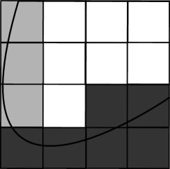
Next, we prove the claim for a general $f\in{\mathcal{C}}(\kappa,M,L,\omega)$. First note that the above arguments apply in the same way to a “vertical horizon model”, i.e., when the roles of the coordinates $x_{1},x_{2}$ are interchanged. Depending on $\kappa$ and on $\omega$, we find next a fixed $I_{0}\in\mathbb{N}$ such that the partition ${\mathcal{P}}_{0}$ comprising the squares $2^{-I_{0}}(D+m)$, $0\leq m_{i}<2^{I_{0}}$, $i=1,2$, can be be decomposed as

$${\mathcal{P}}_{0}={\mathcal{P}}^{v}_{0}\cup{\mathcal{P}}^{h}_{0}$$

in such a way that the corresponding regions

$$D^{v}:=\bigcup\,\{P\in{\mathcal{P}}^{v}_{0}\},\quad D^{h}:=\bigcup\,\{P\in{\mathcal{P}}^{h}_{0}\}$$

have the following properties: each connected segment of $\Gamma\cap D^{v}$, $\Gamma\cap D^{h}$ can be written as the graph of a function in $x_{2}$, $x_{1}$, respectively, with slope bounded by two, and hence satisfies (4.7) on each respective region $\tilde{D}$ (see Figure 4). Since the number of these regions is bounded with a constant depending only on $\kappa$ and on $\omega$, it suffices to verify the claim for each such subdomain. Hence, the claim follows, from the result for the preceding special case with $D$ replaced by $\tilde{D}$, with all constants in the above estimates appropriately rescaled. $\Box$

We conclude this section with a few remarks on possible extensions. The above cartoon class is certainly not the most general one for which an analogous result would hold. For instance, one could permit several components where the constants would also depend on a separation between these components. One could consider a finite number of non-tangential self-intersections of the singularity curve, treating these self-intersections in a similar way as the intersection of $\Gamma$ with the vertical boundary portions in the above proof. As in [14], one could relax the present global $C^{2}$ continuity requirement on $\Gamma$ to piecewise continuity with finitely many pieces or even to $B^{2}_{\infty}(L_{\infty})$-Besov regularity.

4.4. Refinement without merging

The scheme used to prove Theorem 4.1 strongly prioritizes parallelograms in combination with a simple index structure. Moreover, the merging operation supports a sufficiently rapid directional adaptation. The prize to be paid is to dispense with nestedness of the resulting partitions which causes well known drawbacks. In particular, simple multi-resolution concepts, based for instance on Alpert wavelets, are no longer available for non-nested partitions.

As an alternative we discuss next a scheme for generating nested hierarchies of anisotropic partitions comprised of triangles and quadrilaterals only, no longer insisting on the quadrilaterals to be parallelograms. Compared to the construction in Theorem 4.1, this scheme is is easier to code, especially for more complex domains. It is a bisection scheme using the following types of splits (see also [10, 35]). Starting from some initial partition of $D$ consisting of triangles and quadrilaterals, refined partitions are obtained by splitting a given cell $Q$ of a current partition according to one of the following rules, depicted in Figure 5:

1. Connect a vertex with the midpoint of an edge not containing the vertex.

2. Connect two vertices.

3. Connect the midpoints of two edges which, when $Q$ is a quadrilateral, do not share any vertex.

Figure 5. Illustration of the partition rules.

We emphasize that that these rules apply to general quadrilaterals as they involve only connecting vertices or midpoints of edges. It is easily checked that these three refinement rules produce only triangles and quadrilaterals. Moreover, the refinement operators used in the proof of Theorem 4.1 are covered by these rules as special cases. In fact, $R^{an}_{\iota}$ is generated by applying one refinement of type (R3) when $\iota=0$ and two refinements type (R1) when $\iota=\pm 1$. Furthermore, the isotropic refinement operator $R^{iso}$ is generated by applying three type (R3) refinements when $Q$ is a parallelogram and by (R3) (R1) (R3) when $Q$ is a triangle.

We briefly indicate now that the bisection split rules (R1) – (R3) offer, in principle, a sufficiently rapid direction adaptation allowing one to create a nested hierarchy of partitions comprised of triangles and quadrilaterals with the following property: Let ${\mathcal{T}}$ denote a partition obtained through $N$ successive splits from (R1) – (R3), starting from a given initial partition which for simplicity consists just of the unit square. As before, let $\mathbb{P}_{1}({\mathcal{T}})$ denote the space of discontinuous, piecewise linear polynomials on ${\mathcal{T}}$ and $\Sigma_{N}$ the union of all such spaces on such partitions generated by any combination of at most $N$ successive refinements (R1) – (R3).

Theorem 4.3.

For any $f\in{\mathcal{C}}(\kappa,L,M,\omega)$ one has

(4.53) $$\inf_{\varphi\in\Sigma_{N}}\|f-\varphi\|_{L_{2}(D)}\leq C(\log N)N^{-1},\quad N\in\mathbb{N},$$

where $C$ depends only on $\kappa,L,M,\omega$.

We do not insist in (4.53) on the smallest possible power of $\log N$. The purpose of Theorem 4.3 is again to provide a benchmark for which rates could be achieved when adaptively using the above split rules. As in Theorem 4.1 the subsequent proof is constructive but not meant to suggest a practical algorithm because the construction is based on an ideal oracle directing the choice of splits. However, replacing the ideal oracle used below by some a posteriori criteria, as done later below, leads to a practical algorithm whose performance can then be compared with the rates given in Theorem 4.3, see e.g. [7, 8] for algorithms with similar refinement rules. Of course, the number $N$ of splits is a lower bound for the computational work required by any such numerical realization.

Proof: The proof proceeds in three steps. First, we refine isotropically until we achieve the desired target error on all cells that do not not intersect the singularity curve. However, the diameter of these cells is still too large to achieve the target accuracies on the cells intersecting the singularity. Therefore, in a second step, we apply further isotropic refinements to these cells. Finally, in a third step, we ensure the correct parabolic scaling by applying purely anisotropic refinements to the remaining cells intersecting the singularity curve $\Gamma$.

Step 1

We begin with the isotropic partition ${\mathcal{P}}_{J/2}:=(R^{iso})^{J/2}(D)$ (where we assume for simplicity that $J$ is even). Here we assume that $J$ is large enough to ensure that every cell boundary intersects the discontinuity curve just twice, i.e. for every $Q\in{\mathcal{P}}_{J/2}(D)$ with $|Q\cap\Gamma|>0$ we have $\#(\Gamma\cap\partial Q)=2$.

Let ${\mathcal{P}}_{J/2}(\Gamma):=\{Q\in{\mathcal{P}}_{J/2}:|Q\cap\Gamma|>0\}$ be the collection of the cells that intersect the singularity curve on level $J/2$. Then we have

(4.54) $$\inf_{g\in\mathbb{P}_{1}}\|f-g\|_{L_{2}(Q)}^{2}\leq M^{2}2^{-2J}|Q|$$

for all $\,Q\in{\mathcal{P}}_{J/2}\setminus{\mathcal{P}}_{J/2}(\Gamma)$. The total projection error on the union of those squares outside ${\mathcal{P}}_{J/2}(\Gamma)$ is bounded by $M2^{-J}$.

Step 2

In order to obtain the desired diameter for the cells intersecting the singularity, we successively subdivide isotropically only the cells intersecting $\Gamma$ until reaching level $J$. For each refinement level $j$ with $J/2\leq j\leq J$ we have

(4.55) $$\#({\mathcal{P}}_{j}(\Gamma))\leq C2^{j}$$

cells intersecting $\Gamma$, where $C$ depends only on $L,\kappa,\omega$. Each isotropic refinement generates $4$ sub-cells so that we obtain at most

$$\sum_{j=J/2}^{j<J}4C2^{j}\leq 4C2^{J}$$

new sub-cells. Each cell that does not intersect the singularity satisfies the error bound (4.54).

Step 3

Finally, we apply some anisotropic refinements to achieve the parabolic scaling. To simplify the construction note that on each $Q\in{\mathcal{P}}_{J}(\Gamma)$ we can replace $\Gamma\cap Q$ by the straight line connecting the two intersection points $\{p,q\}=\partial Q\cap\Gamma$. In fact the squared error on $Q$ caused this way is easily seen to be bounded by $\bar{C}M^{2}2^{-3J}$ where $\bar{C}$ depends on the curvature bound $\kappa$. Hence, by (4.55), for $J$ larger than $J_{0}$, depending on $L,\kappa,\omega$, the total squared error on the union of all $Q\in{\mathcal{P}}_{J}(\Gamma)$ is bounded by $\bar{C}M^{2}2^{-2J}$ where $\bar{C}$ depends on $\kappa$.

From now on we will therefore assume that $\Gamma$ is a polygon with vertices $p=p(Q),q=q(Q)$ on the boundaries $\partial Q$, i.e., $Q\cap\Gamma$ is a straight line segement contained in $Q$ with end points $p=p(Q),q=q(Q)$ located on $\partial Q$. The goal of the subsequent anisotropic refinements is to create a cell $Q(\Gamma)$ which contains the whole line segment $\Gamma\cap Q$ and has area $\leq 2^{-3J}$, i.e.,

(4.56) $$\Gamma\cap Q\subset Q(\Gamma),\quad|Q(\Gamma)|\leq 2^{-3J}.$$

Since there are $\leq 4C2^{J}$ elements in ${\mathcal{P}}_{J}(\Gamma)$, the total squared error on those squares is then

$$\sum_{Q\in{\mathcal{P}}_{J}(\Gamma)}\inf_{g\in{\mathbb{P}}_{1}}\|f-g\|^{2}_{L_{2}(Q(\Gamma))}\leq 4CM^{2}2^{-2J}\sum_{Q\in{\mathcal{P}}_{J}(\Gamma)}\|f\|^{2}_{L_{2}(Q)},$$

and hence of the desired same order as the total squared error on all cells that do not intersect $\Gamma$. The proof of Theorem 4.3 follows as soon as we have shown that the number of refinements needed to achieve (4.56) is bounded by a fixed absolute multiple of $J$.

We will show next that (4.56) can indeed be achieved at the expense of the order of $J$ further refinements. These refinements will create a sequence of cells $Q_{k}$ with $Q=Q_{0}$, always containing $\Gamma\cap Q$, which are either quadrilaterals or triangles. We refer to the edges $E^{k}_{p},E^{k}_{q}$ of $Q_{k}$ containing $p,q$, respectively, as split-edges. One then encounters one of the following two cases:

(I): The endpoints $p,q$ of $\Gamma\cap Q_{k}$ are located on a pair of opposite split-edges $E^{k}_{p},E^{k}_{q}$ of the quadrilateral $Q_{k}$, i.e., these edges do not have any vertex of $Q_{k}$ in common, see the two cases in Figure 6.

(II): The split-edges $E^{k}_{p},E^{k}_{q}$ of $Q_{k}$, share a common vertex and $Q_{k}$ is either a triangle or a quadrilateral, see Figure 7.

We describe first the refinements for case (I). Figure 6 shows for the initial cell $Q=Q_{0}$ all possible situations modulo a rotation or swapping coordinates.

Figure 6. (Ia): split type (R1);    (Ib): split type (R3)

To simplify the explanation we call the endpoint of $E^{k}_{p},E^{k}_{q}$ which has the larger distance from $p,q$, respectively, its far-vertex. We call this distance the far-distance. In these terms we apply the following rule:

IR: Apply either (R1) or (R3) according to the following conditions:

• If the far-vertex of $E_{p}$ and the far-vertex of $E_{q}$ are not connected by a common edge of $Q_{k}$ apply (R1) by splitting the longest split-edge as indicated in Figure 6, (Ia) (this leaves $\Gamma\cap Q_{k}$ within the new quadrilateral $Q_{k+1}$).

• If the far-vertices of $E^{k}_{p},E^{k}_{q}$ are the endpoints of a common edge of $Q_{k}$, apply (R3) splitting both $E^{k}_{p}$ and $E^{k}_{q}$, see Figure 6, (Ib).

The rule says that one chooses the split that reduces as many far-distances as possible. If one can split only one split-edge one chooses the larger one. The following properties are then an immediate consequence:

IPr: Given $Q_{k}$ of type (I), $Q_{k+1}$ still contains $\Gamma\cap Q$ and is also of type (I). Moreover, either both split-edges are halved, i.e., $|E_{p}^{k+1}|=|E_{p}^{k}|/2$ and $|E_{q}^{k+1}|=|E_{q}^{k}|/2$, or the longer one of the split-edges is halved, i.e., $|E_{p}^{k+1}|=|E_{p}^{k}|/2$ and $|E_{q}^{k+1}|=|E_{q}^{k}|$.

Hence, since the splits aim at reducing far-distances, after at most $2J$ such refinements one has $|E^{J}_{p}|\leq 2^{-2J}$, $|E^{J}_{q}|\leq 2^{-2J}$, i.e., $|Q_{J}|\lesssim 2^{-3J}$, as desired. Thus, in this case the refinement process terminates after at most $2J$ splits and achieves (4.56).

We now turn to case (II) and start with the refinement for $Q_{0}=Q$. First we apply (R2) so that $\Gamma$ is now contained in the triangle $Q_{1}$ spanned by the vertices $x_{ll},x_{ul},x_{ur}$, see Figure 7, (IIa).

Figure 7. $Q_{1}$ is a triangle after (R2) in the case (II)

More generally, whenever $Q_{k}$ is a triangle, up to rotation or swapping coordinates, there are three possible configurations as indicated in Figure 7, namely, denoting again by $x_{ul}=E^{k}_{p}\cap E^{k}_{q}$ the common vertex of the two split-edges:

(IIa): $x_{ul}$ is the far-vertex for both $p$ and $q$, see case (IIa) in Figure 7;

(IIbc): the far-vertex of at least one of the $p,q$ is not $x_{ul}$, see the cases (IIb), (IIc) in Figure 7.

Again the idea is to choose the split that best reduces the far-distances of $p$ and $q$.

In the case (IIa) of Figure 7 we can apply the split (R3), cutting off the far-vertex $x_{ul}$ and leaving $\Gamma\cap Q$ in a quadrilateral $Q_{2}$, where the two far-distances have at least been halved, see Figure 8, (IIa). $Q_{2}$ is now of type (I), so at most $2(J-1)$ further refinements, as described for case (I), are needed to produce $Q(\Gamma)=Q_{2J}$ satisfying (4.56). Thus, in this case the refinement procedure terminates as well with (4.56) after at most $2J$ splits.

Figure 8. Next split generating $Q_{2}$ in the cases (IIa), (IIb), (IIc)

In the case (IIbc) (see cases (IIb) and (IIc) in Figure 8) we can either apply the split (R1) if only one of the far-vertices is different from $x_{ul}$, splitting the midpoint of the respective split-edge, or one applies (R3) if $x_{ul}=E^{k}_{p}\cap E^{k}_{q}$ is not a far-vertex for either one $p$ or $q$, see Figure 8, (IIc). In both cases $Q_{k+1}$ contains $\Gamma\cap Q$ and is again a triangle and hence is of type (IIa) or (IIbc). Moreover, since at least one split-edge is halved one has $|Q_{k+1}|\leq|Q_{k}|/2$. Thus, one can have at most $J$ steps reproducing (IIbc) because such a $Q_{J}$ would have area at most $2^{-J}2^{-2J}=2^{-3J}$. In this case $Q_{J}$ would satisfy (4.56) and the process terminates. So suppose after $J_{0}<J$ refinements $Q_{J_{0}}$ is of type (IIa). As shown above, one additional (R3) split produces a quadrilateral containing $\Gamma\cap Q$ and hence returns to case (I). Moreover, by the above properties, the product of the length of the split-edges of $Q_{J_{0}}$ is at most $2^{-J-J_{0}}$. By the properties IPr of the process for case (I) at most $2J-J_{0}$ additional refinements are needed to reduce both split-edges to length at most $2^{-2J}$. The resulting $Q_{2J}$ again satisfies (4.56) which completes the proof. $\Box$

In (4.53) the error decay is measured in terms of the number of subdivisions which indicates the work needed to generate the partition. On the other hand, the number of splits is proportional to the number of generated cells and thus gives an estimate which is comparable with the one given in Theorem 4.1. In particular, the refinement scheme of this section offers more possibilities with regard to the shape of the cells, but removes the merging in favor of nestedness. Although the results are eventually not sharp, for the given arguments the additional merging allows a slightly better log factor $(\log N)^{1/2}/N$ in Theorem 4.1 as opposed to $(\log N)/N$ in Theorem 4.3. The additional log factor originates from the anisotropic refinements necessary for the direction adaption in Step 3. However, after generating the partition one could merge all those cells in $Q\in{\mathcal{P}}_{J}(\Gamma)$ that are generated in the intermediate directional refinements and which do not intersect $\Gamma$, retaining only $O(2^{J})$ cells. Revisiting the different cases in Step 3, it is easy to see that these merged cells are either triangles or quadrilaterals, still forming a nested hierarchy. Thus an error of order $N^{-1}$ is obtained with $O(N)$ degrees of freedom any numerical algorithm based on the split rules (R1) – (R3) would require a number of operations of at least the order $N\log N$.

4.5. Adaption for transport problems

In this section we combine the general adaptive scheme Algorithm 1 from Section 2.2 with hierarchies of trial spaces based on anisotropic refinements of the type studied in Section 4.3. To this end, we have to find realizations of the functions ExpandStable and Approx which we describe next. The trial spaces $X_{j}$ are spanned by piecewise linear functions on a mesh ${\mathcal{M}}_{j}$ composed of cells from collections $\tilde{{\mathcal{C}}}_{j}$, i.e.,

(4.57) $$X_{j}=\mathbb{P}_{1}(\tilde{\mathcal{C}}_{j}),\quad j\geq 0.$$

The collections $\tilde{\mathcal{C}}_{j}$ consist of anisotropically and isotropically refined cells of the type introduced in the previous subsection. Given $X_{j}$ of the form (4.57), we define the procedure ExpandStable by

$$\textsc{ExpandStable}(X_{j}) =\mathbb{P}_{2}(\tilde{\mathcal{M}}_{j})\cap C(D) \tilde{\mathcal{M}}_{j}:=\{R^{iso}(P):P\in\tilde{\mathcal{C}}_{j}\}\;.$$ where

It will be seen that $\textsc{ExpandStable}(X_{j})$ is large enough to ensure $\delta$-proximality with constant $\delta$ significantly smaller than one.

We next explain the anisotropic adaptive refinement leading to an implementation of the adaption routine Approx in Algorithm 1. The idea is to use a greedy strategy based on the largest “fluctuation coefficients”. To describe this, we first initialize $\tilde{\mathcal{C}}_{j}$ by $\tilde{\mathcal{C}}_{0}={\mathcal{C}}_{0}$ defined as in (4.15). The initial isotropic refinement level $J_{0}$ is typically a small integer but could depend on a priori knowledge about the convection field $\vec{b}$.

Since we have to rely on a refinement criterion that does not have the information used in the proof of Theorem 4.1 we cannot guarantee that any singularity curve intersects only parallelograms. Therefore, given $\tilde{\mathcal{C}}_{j-1}$, $j$ odd, we associate with every $Q\in\tilde{\mathcal{C}}_{j-1}$ the collection ${\mathcal{R}}^{an}_{j}(Q)$ of anisotropic refinements $R_{j}(Q)$ where $R_{j}(Q)$ is defined as follows: $R_{j}(Q)=R^{an}(Q)$ runs through the anisotropic refinements $R^{an}_{\iota}(Q)$, $\iota=0,\pm 1$, defined in (4.10), when $Q$ is a parallelogram. When $Q$ is a triangle, we apply $R^{iso}$ instead. When $j$ is even $R_{j}$ agrees with $R^{iso}$, which is defined for triangles and parallelograms, producing a single isotropic refinement of $Q$ involving either only triangles or parallelograms. We should point out that anisotropic refinement $R^{an}$ is applied only for parallelograms and we always apply isotropic refinement $R^{iso}$ for triangles.

Given $Q\in\tilde{\mathcal{C}}_{j-1}$, we denote for every $R_{j}(Q)$ by $\Psi_{R_{j}(Q)}$ an $L_{2}$-orthonormal basis for $\mathbb{P}_{1}(R_{j}(Q))$. Recall that $A^{*}r^{K}_{j}\in L_{2}(D)$. For $j$ odd, we have to select from several possible anisotropic refinements by

(4.58) $$R^{*}_{j}(Q):=\operatornamewithlimits{argmax}\,\{\|P_{R_{j}(Q)}A^{*}r^{K}_{j}\|_{L_{2}(Q)}:R_{j}(Q)\in{\mathcal{R}}^{an}_{j}(Q)\},$$

where $P_{R_{j}(Q)}$ is the $L_{2}$-orthogonal projector to $\mathbb{P}_{1}(R_{j}(Q))$. When $j$ is even we have $R_{j}^{*}(Q)=R_{j}(Q)$. Then, fixing some $\theta\in(0,1)$ we define the collection ${\mathcal{M}}$ of marked cells in $\tilde{\mathcal{C}}_{j-1}$ by

(4.59) $${\mathcal{M}}(\tilde{\mathcal{C}}_{j-1}):=\{Q\in\tilde{\mathcal{C}}_{j-1}:\|P_{R^{*}_{j}(Q)}A^{*}r^{K}_{j}\|_{L_{2}(Q)}\geq\theta\max_{Q\in\tilde{\mathcal{C}}_{j-1}}\|P_{R^{*}_{j}(Q)}A^{*}r^{K}_{j}\|_{L_{2}(Q)}\}.$$

Then set

(4.60) $$\tilde{\mathcal{C}}_{j}^{0}:=\mbox{MERGE}(\{Q^{\prime}\in R^{*}_{j}(Q):Q\in{\mathcal{M}}(\tilde{\mathcal{C}}_{j-1})\}),\quad\tilde{\mathcal{C}}^{1}_{j}:=\{Q\in\tilde{\mathcal{C}}_{j-1}:Q\notin{\mathcal{M}}(\tilde{\mathcal{C}}_{j-1})\},$$

providing the refined partition

$$\tilde{\mathcal{C}}_{j}:=\tilde{\mathcal{C}}^{0}_{j}\cup\tilde{\mathcal{C}}^{1}_{j}.$$

Here, we can not directly apply the operator MERGE as defined in Lemma 4.2 since the discontinuity curve $\Gamma$ is not known in this case. For our numerical scheme, we newly define $\mbox{MERGE}({\mathcal{C}})$ by a set of cells obtained by merging two triangles created from $R^{an}$ to form a parallelogram if there are any such triangles $Q_{1},Q_{2}\in{\mathcal{C}}$ while keeping other cells $Q\in{\mathcal{C}}$ as they are.

Finally, we have to implement UpdateDataSpace. For simplicity, we use the trivial choice

$$\textsc{UpdateDataSpace}(f,\epsilon,F_{h},X_{h})=(f,X_{h}),$$

which essentially means that we ignore data approximation errors. Our numerical adaptive scheme 2DSOLVER is summarized in Algorithm 2.

Algorithm 2 2DSOLVER

1:Initialization: for given target $L_{2}(D)$-accuracy $\epsilon>0$ choose an initial trial space $X_{0}=\mathbb{P}_{1}(\tilde{\mathcal{C}}_{0})$. Set the initial guess, initial error bound and test space

$$u_{a} =0, errbound =\|f\|_{Y^{\prime}}, Z_{0}=\textsc{ExpandStable}(X_{0}),$$

respectively. Choose parameters $K\in\mathbb{N}$ and $j=0$.

2:while $errbound>\epsilon$ do

3:     Compute $\hat{u}_{a}$, $\hat{r}_{a}$ as the result of $K$ Uzawa iterations with initial value $u_{a}$, right hand side $f$ and test and trial spaces $X_{j}$ and $Z_{j}$.

4:     Compute $\tilde{\mathcal{C}}_{j+1}$ from $\tilde{\mathcal{C}}_{j}$ by (4.60).

5:     $X_{j+1}:=\mathbb{P}_{1}(\tilde{\mathcal{C}}_{j+1})$

6:     $Z_{j+1}:=\textsc{ExpandStable}(X_{j+1})$

7:     Set $j\rightarrow j+1$ and update $u_{a}$ by

$$u_{a}:=\hat{u}_{a}+\sum_{Q\in\tilde{\mathcal{C}}_{j}}P_{Q}A^{*}\hat{r}_{a}.$$

8:     Update $errbound$.

$$errbound:=\Big{(}\sum_{Q\in\tilde{\mathcal{C}}_{j}}\|P_{Q}A^{*}\hat{r}_{a}\|^{2}_{L_{2}(Q)}\Big{)}^{1/2}.$$

9:end while

5. Numerical Experiments

We now provide some numerical experiments to illustrate the performance of the previously introduced anisotropic adaptive scheme for first order linear transport equations. For the numerical tests, we consider two simple transport equations: One with a jump induced by the right hand side and one with a jump induced by the boundary conditions. In both cases the discontinuity curves will be seen to be accurately resolved by relatively few degrees of freedom, showing the effectiveness of the scheme. Moreover, we display numerically estimated values for the stability constant $\delta$ given by

$$\frac{\inf_{\phi\in Z_{j}}\|u_{j}-u_{j}^{K}-A^{*}\phi\|_{L_{2}([0,1]^{2})}}{\|u_{j}-u_{j}^{K}\|_{L_{2}([0,1]^{2})}},$$

where $u_{j}=\text{argmin}_{v_{j}\in X_{j}}\|u-v_{j}\|_{2}$. Using that $\|\cdot\|_{Y}=\|A^{*}\cdot\|_{X}$ this is exactly the constant $\delta$ in the definition (3.5) of $\delta$-proximality, however with $y$ (in (3.5)) replaced by $u_{j}-u_{j}^{K}$. This is of course only a lower bound for the true $\delta$-proximality constant, but the given choice for $y$ is exactly the one used in the proofs in [17].

In the subsequent experiments, the number $K$ of iterations of the adaptive scheme described in Section 3 is for simplicity set to $K=10$. One could as well employ an early termination of the inner iteration based on a posteriori control of the lifted residuals $r^{k}_{j}$.

5.1. Linear Transport Equation with homogeneous inflow data

We first consider a transport equation with zero inflow boundary condition, whose solution exhibits a discontinuity along the curvilinear layer given by $x_{1}=\frac{1}{2}x_{2}^{2}$. More precisely, we consider the equation given by

(5.1) $$Au=\left(\begin{array}[]{c}x_{2}\\ 1\\ \end{array}\right)\cdot u+u=f,\quad f=\chi_{\{x_{1}>x_{2}^{2}/2\}}+1/2\cdot\chi_{\{x_{1}\leq x_{2}^{2}/2\}}.$$

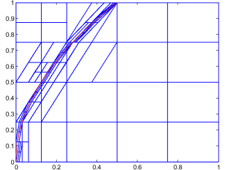
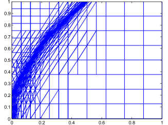
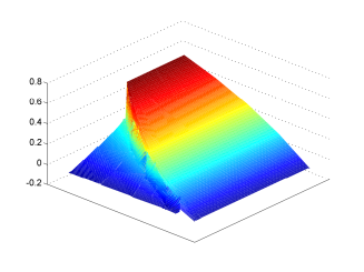
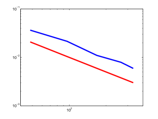
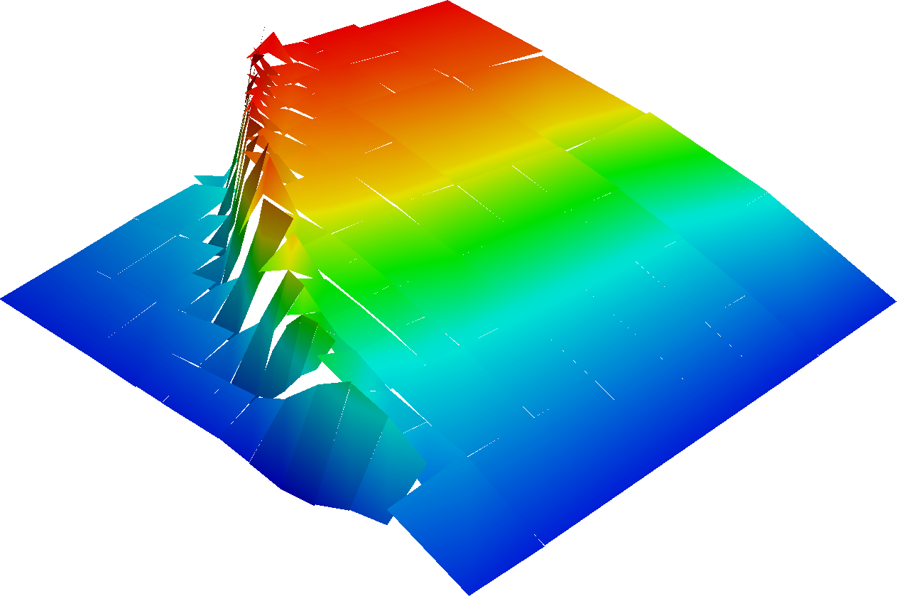
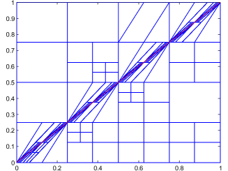
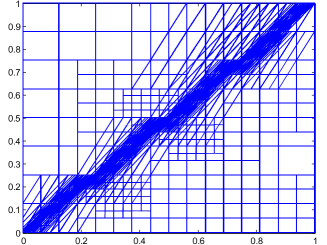
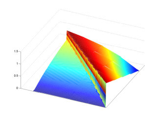
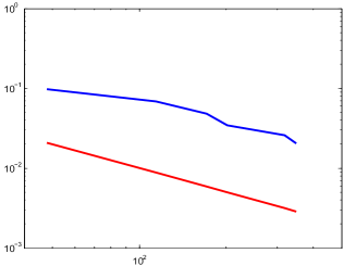
Figure 9 9(a), 9(b) show the adaptive partitions associated with the trial space $X_{5}$ and the test space $Z_{5}$ clearly demonstrating their highly anisotropic structure reflected by the refinements in the neighborhood of the discontinuity curve. Figure 9(c) illustrates the anisotropic approximation given by 306 basis elements. For a comparison, Figure 10 shows the corresponding results with isotropic refinements only. We emphasize that in our scheme, Gibbs like phenomena and spurious oscillations across the jump are almost completely absent and in fact much less pronounced than observed for isotropic discretizations. Figure 9(d) shows the optimality of the anisotropic scheme. The numerical stability is confirmed by Table 1.

(a)

(b)

(c)

(d)

Figure 9. 9(a) Adaptive partition for the trial space $X_{5}$. 9(b) Adaptive partition for the test space $Z_{5}$. 9(c) Approximate solution (306 basis elements). 9(d) Approximation error in $L_{2}(D)$ versus the number of degrees of freedom (blue) and the theoretical rate (red).

Figure 10. Solution and partition of the $8$th isotropically adaptive cycle for the test problem (5.1). The trial space and test spaces consist of linear and bilinear finite elements, respectively. The partition for the test space is obtaind from the corresponding parition for the trial space by refining each cell once.

Anisotropic				Isotropic
$n$	Estimated $\delta$	$L_{2}$ error	Rate	$n$	Estimated $\delta$	$L_{2}$ error	Rate
$48$	$0.3$	$3.65\cdot 10^{-2}$		$52$	$0.25$	$8.93\cdot 10^{-2}$	$0.37$
$99$	$0.44$	$2.15\cdot 10^{-2}$	$0.73$	$100$	$0.26$	$7.54\cdot 10^{-2}$	$0.26$
$138$	$0.35$	$1.39\cdot 10^{-2}$	$1.31$	$160$	$0.29$	$6.53\cdot 10^{-2}$	$0.31$
$177$	$0.32$	$1.09\cdot 10^{-2}$	$0.98$	$256$	$0.33$	$5.49\cdot 10^{-2}$	$0.37$
$237$	$0.32$	$8.35\cdot 10^{-3}$	$0.91$	$388$	$0.38$	$4.87\cdot 10^{-2}$	$0.29$
$306$	$0.31$	$6.15\cdot 10^{-3}$	$1.21$	$556$	$0.44$	$4.4\cdot 10^{-2}$	$0.28$

Table 1. Numerical estimates for the stability constant $\delta$, $L_{2}$ approximation error and estimated convergence rates.

Figure 11. $L_{2}$ errors of Examples (5.1) and (5.2) and a line indicating the rate $n^{-1}$, respectively.

5.2. Linear Transport Equation with inhomogeneous inflow data

Second, as a classical benchmark, we consider a transport equation with non-zero boundary condition, whose solution exhibits a discontinuity along the shear layer given by $x_{1}=x_{2}$. More precisely, we consider the equation given by

(5.2) $$Au=\left(\begin{array}[]{c}1\\ 1\\ \end{array}\right)\cdot u+u=f,\quad f=1/2$$

with boundary conditions

$$g(x_{1},x_{2})=1-x_{1}\,\,\text{on}\,\,\{(x_{1},0)\in\Gamma_{-}:0<x_{1}<1\}$$

and

$$g(x_{1},x_{2})=0\,\,\text{on}\,\,\{(0,x_{2})\in\Gamma_{-}:0<x_{2}<1\}.$$

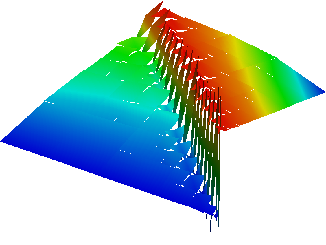
Figures 12 and 13 show the numerical results for the anisotropic and isotropic cases, respectively. As in the previous case the anisotropic solutions show negligible spurious oscillations and are more stable than the isotropic ones. The $L_{2}$ approximation error and $\delta$ estimates can be found in Table 2.

(a)

(b)

(c)

(d)

Figure 12. 12(a) Adaptive partition for the trial space $X_{5}$. 12(b) Adaptive partition for the test space $Z_{5}$. 12(c) Approximate solution (345 basis elements). 12(d) Approximation error in $L_{2}(D)$ versus the number of degrees of freedom (blue) and the theoretical rate (red).

Figure 13. Solution and partition of the $6$th isotropically adaptive cycle for the test problem (5.2). The trial space and test spaces consist of linear and bilinear finite elements, respectively. The partition of the test space is obtaind from the the corresponding partition of the trial space by refining each cell once.

Anisotropic				Isotropic
$n$	Estimated $\delta$	$L_{2}$ error	Rate	$n$	Estimated $\delta$	$L_{2}$ error	Rate
$48$	$0.14$	$9.71\cdot 10^{-2}$		$52$	$0.25$	$8.93\cdot 10^{-2}$	$0.37$
$108$	$0.19$	$6.87\cdot 10^{-2}$	$0.43$	$100$	$0.26$	$7.54\cdot 10^{-2}$	$0.26$
$162$	$0.22$	$4.85\cdot 10^{-2}$	$0.86$	$160$	$0.29$	$6.53\cdot 10^{-2}$	$0.31$
$201$	$0.18$	$3.44\cdot 10^{-2}$	$1.59$	$256$	$0.33$	$5.49\cdot 10^{-2}$	$0.37$
$285$	$0.19$	$2.74\cdot 10^{-2}$	$0.65$	$388$	$0.38$	$4.87\cdot 10^{-2}$	$0.29$
$345$	$0.18$	$2.31\cdot 10^{-2}$	$0.89$	$556$	$0.44$	$4.4\cdot 10^{-2}$	$0.28$

Table 2. Numerical estimates for the stability constant $\delta$, $L_{2}$ approximation error and convergence rates.

In summary, the experiments confirm that the employed anisotropic adaptive refinements essentially recover the optimal rates relating the achieved accuracy to the used number of degrees of freedom. Overall this results in a better rate than the one achieved by isotropic refinements. Perhaps more importantly, the anisotropy appears to greatly promote the stability of the scheme, i.e., the projections form the spaces $Z_{j}$ (although not much larger in dimension than $X_{j}$) come sufficiently close to the optimal (computationally infeasible) test spaces to give rise to very well conditioned variational problems. Moreover, pointwise over- and undershoots of the approximations analogous to Gibbs’ phenomena near jump discontinuities when approximating in $L_{2}(D)$ in these examples is much less pronounced than with isotropic refinements.

6. The Parametric Case

We now consider parametric transport problems of the type (2.9) and adhere to the notation and terminology introduced in Section 2.2. We recall (2.10), i.e. the in- and outflow boundaries

$${\partial D}_{\pm}(\vec{s}):=\{x\in\partial D:\pm\vec{b}(\vec{s})\cdot\vec{n}(x)>0\},\;\;\vec{s}\in{\mathcal{S}},$$

now depend on the transport direction $\vec{s}\in{\mathcal{S}}$. Similar to [22, 23], we will now investigate the possibility of sparse tensor product approximations of the parametric transport problem (2.9)–(2.10), using the directionally adaptive multi-level approximation rates in $L_{2}(D)$ which were obtained in Theorem 4.1.

We outline in this section some circumstances under which the preceding anisotropic approximations lead in connection with sparse tensor product concepts to the efficient computation of simple quantities of interest of the parametric fields $u(\cdot\vec{s})$.

6.1. Sparse Tensor Approximation Rate Estimates

We assume given a continuous, linear functional $G(\cdot)\in(L^{2}(D))^{*}$, independent of the transport direction $\vec{s}$. The goal of computation is now to approximate an integral quantity over all directions $\vec{s}$, such as the total emission:

(6.1) $$I(G(u)):=\int_{\mathcal{S}}G(u(\cdot,\vec{s}))d\vec{s}\;.$$

In order to obtain superior rates of sparse tensor product approximations, we require that the solution $u(\vec{s},x)$ of (2.9)–(2.10) belongs to the cartoon class ${\mathcal{C}}$ uniformly over all directions $\vec{s}$, with a certain amount of regularity with respect to $\vec{s}$. We work under the following assumptions.

Assumption 6.1.

1. Condition (2.2) holds uniformly with respect to the direction $\vec{s}\in{\mathcal{S}}$,

2. There exist parameters $\kappa,L,M,\omega$ (as in Theorem 4.1) such that problem (2.9) admits for each $\vec{s}\in{\mathcal{S}}$ a unique solution $u(\vec{s},\cdot)\in{\mathcal{C}}(\kappa,L,M,\omega)$ and

3. $G\circ u\in C^{0,\alpha}({\mathcal{S}})$ for some $0<\alpha\leq 1$. We remark that this requirement necessitates regularity with respect to $\vec{s}\in{\mathcal{S}}$ and in the class ${\mathcal{C}}$ of admissible cartoons.

Note that for (uniformly in $\vec{s}$) $C^{1}$-convection fields, piecewise smooth boundary conditions and data $f$ in a cartoon class with $C^{1}$-pieces separated by a $C^{2}$-curve, the solutions belong to a cartoon class with parameters depending on the data (right hand side, boundary data, convection field) and thus satisfies Assumption 6.1(2). We assume we have at hand a family $\{I_{\ell}\}_{\ell\geq 0}$ of quadrature approximations to the direction-integral $I$ in (6.1) which, for integrand functions $\varphi\in C^{0,\alpha}({\mathcal{S}})$, for some $0<\alpha\leq 1$, converges with $O(h_{\ell}^{\alpha})$

(6.2) $$\left|I(\varphi)-I_{\ell}(\varphi)\right|\lesssim h^{\alpha}_{\ell}|\varphi|_{C_{h_{\ell}}^{0,\alpha}({\mathcal{S}})},\quad\ell\to\infty,\;.$$

where $|\varphi|_{C_{h}^{0,\alpha}({\mathcal{S}})}:=\sup_{\vec{s},\vec{s}^{\prime}:|\vec{s}-\vec{s}^{\prime}|\geq h}|\vec{s}-\vec{s}^{\prime}|^{-\alpha}|\varphi(\vec{s})-\varphi(\vec{s}^{\prime})|$ is a “conditional” Lipschitz semi-norm which is for $h>0$ weaker than $\|\varphi\|_{C^{0,\alpha}({\mathcal{S}})}$. The composed Midpoint- and Trapezoidal rules satisfy (6.2).

For $j\geq 0$, and for $u\in{\mathcal{C}}\subset L^{2}(D)$, we denote by $B^{x}_{j}u$ the anisotropic (and hence nonlinear) approximations constructed in Theorem 4.1 such that there exists a constant $C>0$ such that for all $J\geq 1$

(6.3) $$\|u-B_{J}u\|_{L_{\infty}({\mathcal{S}};L_{2}(D))}\leq CJ^{1/2}2^{-J}\;.$$

We recall that the constant $C$ depends only on the cartoon parameters.

For a favorable sparse approximation error bound, we require the stronger condition that there exists $C>0$ independent of $j$ such that

(6.4) $$|G\circ(u-(B_{j}u)(\vec{s},\cdot))|\leq C|\vec{s}-\vec{s}^{\prime}|^{\alpha}j^{1/2}2^{-j},\quad\forall\vec{s},\vec{s}^{\prime}\in{\mathcal{S}}\,\mbox{ s.t. }|\vec{s}-\vec{s}^{\prime}|\geq 2^{-j}\;.$$

This assumption is deliberately optimistic because its consequences will later just serve as a benchmark for the subsequent numerical realizations.

The quadrature approximation $I_{L}$ of the integral over ${\mathcal{S}}$ is based on $N^{s}_{L}=O(2^{L})$ (usually equi-spaced in ${\mathcal{S}}$) directions $\vec{s}$, denoted by $\vec{s}^{\ell}_{i}\in{\mathcal{S}}$, $i=1,...,N^{s}_{\ell}=O(2^{\ell})$. We define

$$\delta I_{\ell}:=I_{\ell}-I_{\ell-1}\;,\quad\ell=0,1,...$$

with the convention $I_{-1}:=0$. Then, for every $L\geq 1$,

$$I_{L}=\sum_{\ell=0}^{L}\delta I_{\ell}\;,\quad\mbox{where}\quad\delta I_{\ell}:=(I_{\ell}-I_{\ell-1})\;.$$

We approximate $I(G(u))$ by

(6.5) $$I_{L}(G(u);\{j(\ell)\}_{\ell=0}^{L}):=\sum_{\ell=0}^{L}(\delta I_{\ell}(G(u_{j(\ell)})))$$

i.e., by quadrature-differences $\delta I_{\ell}$ applied to (functionals of) anisotropically approximated solutions in the spatial domain $D$, with spacial resolution level $j(\ell)$ to be determined. Note that each $\delta I_{\ell}$ requires evaluating $G(u)$ at $O(2^{\ell})$ distinct directions $\{\vec{s}^{\ell}_{i}\}_{i=1}^{N^{s}_{\ell}}$ with $N^{s}_{\ell}=O(2^{\ell})$. Each of these evaluations $G(u(\cdot,\vec{s}^{\ell}_{i}))$ can be done by approximating $u(\cdot,\vec{s}^{\ell}_{i})$ in $L^{2}(D)$. Then evaluating $G()$ on this approximation (which we assume to be possible in $O(2^{j(\ell)})$ operations we subsequently form $\delta I_{\ell}$. Since we are only interested in an integral functional $G()$, there is no need to merge partitions which are adapted to different directions. We estimate the error

$$E_{L}:=\left|I(G(u))-\sum_{\ell=0}^{L}(\delta I_{\ell}(G(u_{j(\ell)})))\right|\;,$$

and in doing so, we obtain a choice for $j(\ell)$. To this end, we write

$$\begin{array}[]{rcl}E_{L}&\leq&\displaystyle\left|I(G(u))-I_{L}(G(u))\right|+\left|I_{L}(G(u))-\sum_{\ell=0}^{L}(\delta I_{\ell})(G(u_{j(\ell)}))\right|\;.\end{array}$$

The first term, denoted by $E^{1}_{L}$, is bounded by $\lesssim 2^{-\alpha L}$ provided that $\vec{s}\mapsto G(u(\cdot,\vec{s}))\in C^{0,\alpha}({\mathcal{S}})$ which is Assumption 6.1(3). We estimate next the second term, denoted by $E^{2}_{L}$.

Using the linearity of $\delta I_{\ell}$ and of $G()$,

$$\begin{array}[]{rcl}E^{2}_{L}&=&\displaystyle\left|\sum_{\ell=0}^{L}(\delta I_{\ell})(G(u))-(\delta I_{\ell})(G(u_{j(\ell)}))\right|\leq\sum_{\ell=0}^{L}\left|(\delta I_{\ell})(G(u)-G(u_{j(\ell)}))\right|\\ &=&\displaystyle\sum_{\ell=0}^{L}\left|(\delta I_{\ell})(G(u-u_{j(\ell)}))\right|\;.\end{array}$$

We use the error bounds for the quadrature operator, (6.2), and the triangle inequality to infer

$$\begin{array}[]{rcl}\left|(\delta I_{\ell})(G(u-u_{j(\ell)}))\right|&\leq&\displaystyle\left|(I-I_{\ell})(G(u-u_{j(\ell)}))\right|+\left|(I-I_{\ell-1})(G(u-u_{j(\ell-1)}))\right|\\ &\lesssim&\displaystyle 2^{-\alpha\ell}\|G(u-u_{j(\ell)})\|_{C_{2^{-j(\ell)}}^{0,\alpha}({\mathcal{S}})}\\ &\lesssim&\displaystyle 2^{-\alpha\ell}j(\ell)^{1/2}2^{-j(\ell)},\end{array}$$

where we have invoked (6.4) in the last step. We now choose

(6.6) $$j(\ell)\simeq\alpha(L-\ell)\;,\quad L\geq 1\;,\;\;\ell=0,1,...,L$$

and find

$$E^{2}_{L}\leq\sum_{\ell=0}^{L}\left|(\delta I_{\ell})(G(u-u_{j(\ell)}))\right|=2^{-\alpha L}\sum_{\ell=0}^{L}(L-\ell)^{1/2}\lesssim L^{3/2}2^{-\alpha L}\;.$$

Combining with the bound $E^{1}_{L}\lesssim 2^{-\alpha L}$, we arrive at the error bound

(6.7) $$E_{L}\lesssim L^{3/2}2^{-\alpha L}\;.$$

The total number of degrees of freedom/ total work to construct the approximation (6.5) is bounded by (assuming that $G(u_{j})$ can be evaluated to accuracy $O(2^{-\alpha L})$ at a computational cost that stays proportional to the number of degrees of freedom $N^{x}_{j}=O(2^{j})$ involved in building the direction-adaptive approximation $B^{x}_{j}u$ of $u$ in $L^{2}(D)$),

(6.8) $$W_{L}\lesssim\sum_{\ell=0}^{L}2^{\ell}2^{j(\ell)}\simeq\sum_{\ell=0}^{L}2^{\ell}2^{\alpha(L-\ell)}\lesssim L^{\theta(\alpha)}2^{L}\;,$$

with $\theta(\alpha)=0$ if $0<\alpha<1$ and $\theta(1)=1$.

This complexity bound, obtained under the assumption (6.4), will serve as a benchmark for the actual performance of such a sparse-tensor product scheme when combined with the adaptive solver 2DSOLVERdescribed in Section 4.5 and tested for a single convection field in Section 5.

Combining (6.7) and (6.8), we obtain essentially (up to logarithmic terms) the same error versus work bound as for the approximation of the solution in $L^{2}(D)$ for a single transport direction. Then the approximations to $u(\cdot,\vec{s})$ will, of course, not be those constructed in Theorem 4.1, but will be generated adaptively without prior knowledge on $u(\cdot,\vec{s})$, and without certified (quasi-)optimality of the adaptive algorithm.

Notice that this argument did not use the particular construction in Theorem 4.1, and the same reasoning applies to any other directionally adaptive approximation provided that it yields the above rates (6.3) and (6.4).

Also remark that in [22, 23], we obtained approximation rates in $L^{2}({\mathcal{S}}\times D)$ which scaled (up to log terms) analogous to approximation rates of adaptively refined, isotropic approximations in $D$; these rates are, for piecwise linear polynomial approximations in $D$, for parametric transport problems, inferior to the rates furnished by the approximation result, Theorem 4.1.

The rates in [22, 23] were possible due to the adaptive refinements in $D$ being isotropic. Applying the same reasoning as in [22, 23] in the context of directionally adaptive approximations $B^{x}_{j}u$ of the solution $u(\cdot,\vec{s})$ to refinement level $j$ in the domain $D$ which is furnished by Theorem 4.1 to achieve an $L^{2}(D\times{\mathcal{S}})$-rate could increase the asymptotic complexity of the approximation, due to merging the non-nested, directionally adapted partitions in $D$ with directions sweeping all of ${\mathcal{S}}$. The evaluation of $G(B^{x}_{j}u(\cdot,\vec{s}^{\ell}_{i}))$ for each “quadrature node” $\vec{s}^{\ell}_{i}\in{\mathcal{S}}$ which arises in the quadrature approximations obviates this merging step, and affords the work bound (6.8).

6.2. Numerical Experiment

We consider a model parametric transport problem with non-zero inflow boundary data, whose solution exhibits a discontinuity along the $C^{2}$ singular support curve given by $x_{1}=\frac{\tan\theta}{2}x^{2}_{2}$ with $\theta\in[0,\frac{\pi}{4}]$. More precisely, we consider the equation given by

(6.9) $$Au=\left(\begin{array}[]{c}\tan\theta x_{2}\\ 1\\ \end{array}\right)\cdot\nabla u+u=1$$

with boundary conditions

$$g(x_{1},x_{2})=1-x_{1}\,\,\text{on}\,\,\{(x_{1},0)\in\Gamma_{-}:0<x_{1}<1\}$$

and

$$g(x_{1},x_{2})=0\,\,\text{on}\,\,\{(0,x_{2})\in\Gamma_{-}:0<x_{2}<1\}$$

for $\vec{s}=(\cos\theta,\sin\theta)\in{\mathcal{S}}={\mathbb{S}}^{1}$ with $\theta\in[0,\tfrac{\pi}{4}]$. Writing $u(\theta)=u(\vec{s},\cdot)$, we approximate

$$I(G(u)):=\int_{[0,\frac{\pi}{4}]}G(u(\cdot,\theta))d\theta$$

by

(6.10) $$\hat{I}_{L}(G(u))=\sum_{\ell=0}^{L}I_{\ell}(G(u_{j(\ell)}))-I_{\ell-1}(G(u_{j(\ell)})),$$

where $I_{\ell}$ is quadrature approximation of the integral over $[0,\frac{\pi}{4}]$ with $2^{\ell}$ equi-spaced samples in $[0,\frac{\pi}{4}]$ for $\ell\geq 0$ and $I_{-1}=0$. That is

(6.11) $$I_{\ell}(G(u_{j(\ell)}))=\frac{\pi}{2^{\ell+2}}\sum_{i=0}^{2^{\ell}-1}G(u_{j(\ell)}(\cdot,\theta^{\ell}_{i}))\quad\text{and}\quad I_{\ell-1}(G(u_{j(\ell)}))=\frac{\pi}{2^{\ell+1}}\sum_{i=0}^{2^{\ell-1}-1}G(u_{j(\ell)}(\cdot,\theta^{\ell-1}_{i}))$$

where $j(\ell)=L-\ell$, $\theta^{\ell}_{i}=\frac{i\pi}{2^{\ell+2}}$ and $u_{j(\ell)}(\cdot,\theta^{\ell}_{i})$ is an approximate solution to (6.9) for a fixed $\theta^{\ell}_{i}\in[0,\pi/4]$ obtained by our adaptive refinement solver 2DSOLVER with $O(2^{j(\ell)})$ adpatively chosen basis elements. Here, the linear functional $G\in(L_{2}(D))^{*}$ is given as

(6.12) $$G(u)=\int_{D_{0}}u(x)dx\quad\text{where}\,\,D_{0}=[\tfrac{1}{8},\tfrac{5}{8}]\times[\tfrac{1}{4},\tfrac{3}{4}]\;.$$

Note that we choose $D_{0}\subset D$ so that it contains a region where the jump discontinuity of a solution $u$ for (6.9) occurs for each $\theta\in[0,\tfrac{\pi}{4}]$.

Assuming available a directionally adaptive Petrov-Galerkin solver 2DSOLVER in the physical domain, (6.5) is implemented as follows: we assume that subroutine 2DSOLVER requires $N_{\ell}$, an upper bound on the number of basis elements to be activated by 2DSOLVER and the directional angle $\theta\in[0,\tfrac{\pi}{4}]$ as input arguments, to compute $\hat{I}_{L}$ from (6.5) and (6.6).

Algorithm 3

1:

2:Initialization: Choose a maximal refinement level $L>0$.

3:Compute $u_{j(0)}(\cdot,0):=\textsc{2DSOLVER}(N_{0},0)$ with $N_{0}=O(2^{L})$.

4:Compute $G(u_{j(0)}(\cdot,0))$.

5:Apply quadrature approximation (6.11) to compute $I_{0}(G(u_{j(0)}))$.

6:$\hat{I}_{L}\leftarrow I_{0}(G(u_{j(0)}))$.

7:for $\ell=L,\dots,1$ do

8:     Compute $u_{j(\ell)}(\cdot,\theta^{\ell}_{i}):=\textsc{2DSOLVER}(N_{\ell},\theta^{\ell}_{i})$ for $i=0,\dots,2^{\ell}-1$ and $N_{\ell}=O(2^{L-\ell})$.

9:     Compute $G(u_{j(\ell)}(\cdot,\theta^{\ell}_{i}))$ for $i=0,\dots,2^{\ell}-1$.

10:     Apply quadrature approximation (6.11) to compute $I_{\ell}(G(u_{j(\ell)}))-I_{\ell-1}(G(u_{j(\ell)}))$.

11:     $\hat{I}_{L}\leftarrow\hat{I}_{L}+I_{\ell}(G(u_{j(\ell)}))-I_{\ell-1}(G(u_{j(\ell)}))$.

12:end for

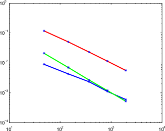
Figure 14 and Table 3 show approximation errors and their comparison with the benchmark rates $n^{-1}$ and $\log_{2}(n)n^{-1}$ for

$$E_{L}=|I(G(u))-\hat{I}_{L}(G(u))|.$$

Dof: $n$	$n^{-1}$ ($\log_{2}(n)n^{-1}$)	$E_{L}$
48	0.020833 (0.116353)	0.012404
144	0.006944 (0.049791)	0.005242
372	0.002688 (0.022954)	0.002407
849	0.001177 (0.003613)	0.001266
1944	0.000514 (0.001842)	0.000740

Table 3. Numerical estimates for the benchmark rates $n^{-1}$ and $\log_{2}(n)n^{-1}$ and the approximation error.

Figure 14. Estimated approximation error in $L^{2}(D)$ versus total number of degrees of freedom (blue), and the benchmark rates $n^{-1}$ (green) and $\log_{2}(n)n^{-1}$ (red).

References

- [1] C. Bardos, Problèmes aux limites pour les équations aux dérivées partielles du premier ordre à coefficients réels; théorèmes d’approximation; application à l’équation de transport, Ann. Sci. Éc. Norm. Supér. 3 (1970), 185–233.
- [2] J.W. Barrett and K.W. Morton, Approximate symmetrization and Petrov-Galerkin methods for diffusion-convection problems, Comput. Methods Appl. Mech. Engrg. 45 (1984), 97–122.
- [3] S. Bougleux, G. Peyré, and L. Cohen, Image compression with anisotropic triangulations, 12th International Conference on Computer Vision, 2009, IEEE, 2343–2348.
- [4] Z. Cai, T. Manteuffel, S. McCormick, and J. Ruge, First-order system : scalar elliptic partial differential equtions, SIAM J. Numer. Anal. 39 (2001), 1418–1445.
- [5] E. Candès and L. Demanet, The curvelet representation of wave propagators is optimally sparse, Comm. Pure Appl. Math. 58 (2005), 1472–1528.
- [6] L. Chen, P. Sun, and J. Xu, Optimal anisotropic simplicial meshes for minimizing interpolation errors in norm, Math. Comp. 76(257) (2007), 179–204.
- [7] A. Cohen, N. Dyn, F. Hecht, and J.-M. Mirebeau, Adaptive multiresolution analysis based on anisotropic triangulations, Math. Comput. 81 (2012), 789–810.
- [8] A. Cohen and J.-M. Mirebeau, Greedy bisection generates optimally adapted triangulations, Math. Comp. 81 (2012), 811–837.
- [9] A. Cohen and J.-M. Mirebeau, Anisotropic smoothness classes: from finite element approximation to image models, J. Math. Imaging Vision 38 (2010), 52–69.
- [10] A. Cohen and J.-M. Mirebeau, private communication, 2013.
- [11] S. Dekel, D. Leviatan, and M. Sharir, On bivariate smoothness spaces associated with nonlinear approximation, Constr. Approx. 20 (2004), 625–646.
- [12] L. Demaret and A. Iske, Anisotropic triangulation methods in adaptive image approximation, In: Approximation Algorithms for Complex Systems, E.H. Georgoulis, A. Iske, and J. Levesley (eds.), Springer, Berlin, 2011, 47–68.
- [13] V. Dolejsi, Anisotropic mesh adaptation for finite volume and finite element methods on triangular meshes, Comput. Vis. Sci. 1 (1998), 165–178.
- [14] E.J. Candès and D. L. Donoho, New tight frames of curvelets and optimal representations of objects with piecewise- singularities, Comm. Pure Appl. Math. 57 (2004), 219–266.
- [15] A. Cohen, W. Dahmen, and R. DeVore, Adaptive frame methods for elliptic operator equations: The steepest descent approach, Math. Comp. 70 (2001), 27–75.
- [16] S. Dahlke, M. Fornasier, T. Raasch, R. Stevenson, M. Werner, Adaptive Frame Methods for Elliptic Operator Equations: The Steepest Descent Approach, IMA J. Numer. Anal. 27(4) (2007), 717–740.
- [17] W. Dahmen, C. Huang, Ch. Schwab, and G. Welper, Adaptive Petrov-Galerkin methods for first order transport equations, SIAM J. Numer. Anal. 50(5) (2012), 2420–2445.
- [18] L. F. Demkowicz and J. Gopalakrishnan, A class of discontinuous Petrov-Galerkin Methods I: The transport equation, Comput. Methods Appl. Mech. Engrg. 199 (2010), 1558–1572.
- [19] L. Demkowicz and J. Gopalakrishnan, A class of discontinuous Petrov-Galerkin methods. Part II: Optimal test functions, Numer. Methods Partial Differential Equations 27 (2011), 70–105.
- [20] D. L. Donoho, Sparse components of images and optimal atomic decompositions, Constr. Approx. 17(3) (2001), 353–382.
- [21] K. Grella, Sparse tensor phase space Galerkin approximation for radiative transport, SpringerPlus, 3, 230, (2014), doi = http://dx.doi.org/10.1186/2193-1801-3-230
- [22] K. Grella and Ch. Schwab, Sparse tensor spherical harmonics approximation in radiative transfer, J. Comput. Phys. 230(23) (2011), 8452–8473.
- [23] K. Grella and Ch. Schwab, Sparse discrete ordinates method in radiative transfer, Comput. Methods Appl. Math. 11(3) (2011), 305–326.
- [24] P. Grohs and G. Kutyniok, Parabolic Molecules, Found. Comput. Math. 14 (2014), 299–337.
- [25] P. Grohs, G. Kutyniok, J. Ma, and P. Petersen, Anisotropic multiscale systems on bounded domains, preprint.
- [26] G. Kutyniok and D. Labate, Resolution of the wavefront set using continuous shearlets, Trans. Amer. Math. Soc. 361 (2009), 2719–2754.
- [27] P. Kittipoom, G. Kutyniok, and W.-Q Lim, Construction of compactly supported shearlet frames, Constr. Approx. 35 (2012), 21–72.
- [28] G. Kutyniok and D. Labate, Shearlets: Multiscale analysis for multivariate data, Birkhäuser Boston, 2012.
- [29] G. Kutyniok, J. Lemvig, and W.-Q Lim, Optimally sparse approximations of 3D functions by compactly supported shearlet frames, SIAM J. Math. Anal. 44 (2012), 2962–3017.
- [30] G. Kutyniok and W.-Q Lim, Compactly supported shearlets are optimally sparse, J. Approx. Theory 163 (2011), 1564–1589.
- [31] W.-Q Lim, The discrete shearlet transform: A new directional transform and compactly supported shearlet frames, IEEE Trans. Image Process. 19 (2010), 1166–1180.
- [32] T. A. Manteuffel, S. McCormick, J. Ruge, and J. G. Schmidt, First-order system for general scalar elliptic problems in the plane, SIAM J. Numer. Anal. 43 (2005), 2098–2120.
- [33] T. A. Manteuffel, K.J. Ressel, and G. Starke, A boundary functional for the least-squares fnite-element solution of the neutron transport problems, SIAM J. Numer. Anal. 37 (2000), 556–586.
- [34] J.-M. Mirebeau, Optimally adapted meshes for finite elements of arbitrary order and norms, Numer. Math. 120(2) (2012), 271–305.
- [35] J.-M. Mirebeau, Adaptive and anisotropic finite element approximation: Theory and algorithms, PhD thesis, Université Pierre et Marie Curie - Paris VI (2011) http://tel.archives-ouvertes.fr/tel-00544243.
- [36] G. Widmer, R. Hiptmair, and Ch. Schwab, Sparse adaptive finite elements for radiative transfer. J. Comput. Phys. 227 (2008), 6071–6105. http://dx.doi.org/10.1016/j.jcp.2008.02.025.
- [37] G. Widmer. Sparse finite elements for radiative transfer, PhD thesis, ETH Zürich, 2009, No. 18420. http://dx.doi.org/10.3929/ethz-a-005916456.