The NH₂D hyperfine structure revealed by astrophysical observations

Abstract

Context. The 1₁₁-1₀₁ lines of ortho and para–NH₂D (o/p-NH₂D), respectively at 86 and 110 GHz, are commonly observed to provide constraints on the deuterium fractionation in the interstellar medium. In cold regions, the hyperfine structure due to the nitrogen (¹⁴N) nucleus is resolved. To date, this splitting is the only one which is taken into account in the NH₂D column density estimates.

Aims. We investigate how the inclusion of the hyperfine splitting caused by the deuterium (D) nucleus affects the analysis of the rotational lines of NH₂D.

Methods. We present 30m IRAM observations of the above mentioned lines, as well as APEX o/p-NH₂D observations of the 1₀₁-0₀₀ lines at 333 GHz. The hyperfine patterns of the observed lines were calculated taking into account the splitting induced by the D nucleus. The analysis then relies on line lists that either neglect or take into account the splitting induced by the D nucleus.

Results. The hyperfine spectra are first analyzed with a line list that only includes the hyperfine splitting due to the ¹⁴N nucleus. We find inconsistencies between the line widths of the 1₀₁-0₀₀ and 1₁₁-1₀₁ lines, the latter being larger by a factor of $\sim$1.6$\pm 0.3$. Such a large difference is unexpected given the two sets of lines are likely to originate from the same region. We next employ a newly computed line list for the o/p-NH₂D transitions, where the hyperfine structure induced by both nitrogen and deuterium nuclei is included. With this new line list, the analysis of the previous spectra leads to linewidths which are compatible.

Conclusions. Neglecting the hyperfine structure owing to D leads to overestimate the linewidths of the o/p-NH₂D lines at 3 mm. The error for a cold molecular core is about 50%. This error propagates directly to the column density estimate. It is therefore recommended to take into account the hyperfine splittings caused by both the ¹⁴N and D nuclei in any analysis relying on these lines.

1 Introduction

The first firm identification of singly deuterated interstellar ammonia, NH₂D, was reported by Olberg et al. (1985) towards three molecular clouds at 86 and 110 GHz, the frequencies of the $J_{K_{a},K_{c}}$=1₁₁-1₀₁ lines of o/p-NH₂D, respectively. The identification was unambiguous thanks to the narrow linewidths which allowed to resolve the hyperfine splitting due to the nitrogen nucleus. These two lines have since been detected in a variety of cold astronomical sources and they are routinely employed to derive the (D/H) ratio in ammonia (see e.g. Roueff et al., 2005). This ratio is a sensitive tracer of the physical conditions and provides strong constraints to deuterium fractionation models.

In the previous studies by Coudert & Roueff (2006, 2009) and in the current spectroscopic databases (JPL and CDMS), the line lists of the NH₂D microwave spectra are based on the measurements by De Lucia & Helminger (1975), Cohen & Pickett (1982) and Fusina et al. (1988). These data sets only consider the nitrogen quadrupole hyperfine structure. In this letter, a new theoretical analysis of the NH₂D hyperfine structure is presented which takes into account the nitrogen quadrupole interaction, the deuteron quadrupole interaction and the nitrogen spin-rotation interaction. It is based on the measurements by Kukolich (1968), Cohen & Pickett (1982), and Fusina et al. (1988). We show that the inclusion of the three coupling terms in the analysis provides a simple explanation for the origin of different linewidths in the 1₀₁-0₀₀ and 1₁₁-1₀₁ lines of NH₂D, as observed recently towards the prestellar core H-MM1. Historically, the first astronomical observation resolving the hyperfine splitting owing to the D quadrupole coupling was presented by Caselli & Dore (2005) for DCO⁺.

The paper is organized as follows. In Sect. 2, we describe the IRAM and APEX observations of the o/p–NH₂D lines detected towards H-MM1. Sect. 3 gives the details of the spectroscopy calculations. In Sect. 4, we discuss the impact of the new line list on the derivation of radiative transition parameters and we conclude in Sect. 5.

2 Observations

The target of the present NH₂D observations is the dense, starless core H-MM1 lying in the eastern part of Lynds 1688 in Ophiuchus (Johnstone et al. 2004; Parise et al. 2011). The position observed, $\alpha$=$16^{\rm h}27^{\rm m}59\aas@@fstack{s}0$, $\delta$=$-24\degr 33\arcmin 33\arcsec$, was chosen as the H₂ column density peak, as derived from pipeline-reduced Herschel far-infrared maps. These were downloaded from the Herschel Science Archive.

2.1 APEX 12m

The ground-state $1_{01}$–$0_{00}$ transitions of o/p-NH₂D at $\sim$333 GHz were observed using the upgraded version of the First Light APEX Submillimeter Heterodyne instrument (FLASH; Heyminck et al., 2006) on APEX (Güsten et al., 2006). The two lines separated by about 40 MHz were covered by one of the MPIfR Fast Fourier Transform Spectrometers (XFTTS) connected to the 0.8 mm receiver. The original spectral resolution at 333 GHz is about 35 m s^-1; the spectra shown in this paper are Hanning smoothed to a resolution of 69 m s^-1 (76 kHz). The APEX beam size (FWHM) is $\sim$20$\arcsec$ at 333 GHz. The observations were carried out between 29 and 31 May, 2015 in stable and fairly good weather conditions (PWV 0.7-1.2 mm), using position switching for sky subtraction. The average system temperature at 333 GHz was 260 K. The resulting RMS noise at a resolution of 69 m s^-1 is 0.017 K on the $T_{\rm A}^{*}$ scale.

2.2 IRAM 30m

The $1_{11}$-$1_{01}$ lines of o/p-NH₂D at $\sim$86 and $\sim$110 GHz were observed at the IRAM 30m telescope using the EMIR 090 receiver and the VESPA autocorrelator. The spectral resolution of this instrument, 20 kHz, is 68 m s^-1 at 86 GHz and $53$ m s^-1 at 110 GHz. At these frequencies, the beam sizes of the telescope are $29\arcsec$ and $23\arcsec$, respectively. The observations were performed on July 5, 2015, in acceptable weather conditions (PWV 8–10 mm). The observing mode was position switching. The integration times for the o/p-NH₂D lines were 15 and 22 minutes, and the average system temperatures at 86 and 110 GHz were 170 K and 250 K, respectively. The resulting RMS noise levels of the o/p–NH₂D spectra were 0.07 K and 0.08 K on the $T_{\rm A}^{*}$ scale.

3 Hyperfine pattern calculations

Just like in NH₃, the nitrogen nucleus in NH₂D can tunnel across the plane made by the H and D nuclei. Each rotational transition is thus split into a doublet by this inversion motion. The resulting rotation-inversion levels are either symmetric or anti-symmetric under the exchange of the two protons and they will either correspond to para or ortho level.

Hyperfine patterns were calculated from a fit of high-resolution data that can be divided into three sets. The first set consists of microwave and far infrared transitions involving the two inversion substates of the ground vibrational state. This first set includes 174 microwave transitions (Cohen & Pickett, 1982) and 297 far infrared transitions (Fusina et al., 1988) for which no hyperfine structure is resolved. The second set involves the 76 microwave transitions listed in Table IX of Cohen & Pickett (1982) for which the nitrogen atom quadrupole coupling structure is resolved. The last data set comprises the 21 hyperfine components measured by Kukolich (1968) for the para $4_{14}$-$4_{04}$ rotation-inversion transition at 25 023.8 MHz. For this last data set, the quadrupole coupling structure due to both the nitrogen and deuterium atoms is resolved.

Rotation-inversion energies were computed with the help of a semi-rigid rotator Hamiltonian for both inversion substates and a second order Coriolis coupling term between these substates (Cohen & Pickett, 1982). Molecule-fixed components of the hyperfine coupling tensors are written using the IAM axis system of this reference. Quadrupole and magnetic spin-rotation hyperfine couplings were taken into account leading to a hyperfine Hamiltonian depending on four coupling constants: two for the quadrupole coupling of the nitrogen and deuterium atoms and two for the magnetic spin-rotation coupling of the same atoms. Using equations similar to Eqs. (3) and (17) of Thaddeus et al. (1964), these four constants can be expressed as diagonal matrix elements of four operators involving four rank two hyperfine coupling tensors: the zero trace ${\bf\chi}^{{\rm N}}$ and ${\bf\chi}^{{\rm D}}$, describing quadrupole coupling of the nitrogen and deuterium atoms, respectively, and ${\bf C}^{{\rm N}}$ and ${\bf C}^{{\rm D}}$, corresponding to the magnetic spin-rotation coupling of the same atoms.

Hyperfine energies were calculated taking the coupling scheme: ${\bf J}+{\bf I}_{{\rm N}}={\bf F}_{1}$ and ${\bf F}_{1}+{\bf I}_{{\rm D}}={\bf F}$ where ${\bf J}$ is the rotational angular momentum, and ${\bf I}_{{\rm N}}$ and ${\bf I}_{{\rm D}}$ are angular momenta of the nitrogen and deuterium nuclei, respectively. The corresponding coupled basis set functions $|J,I_{{\rm N}};F_{1},I_{{\rm D}};F,M_{F}\rangle$ were used to setup the hyperfine Hamiltonian matrix. Matrix elements were taken from Thaddeus et al. (1964).

The inversion-rotation transitions belonging to the first data set were analyzed first allowing us to determine a set of spectroscopic parameters analogous to that listed in Table III of Cohen & Pickett (1982). Components of the four hyperfine coupling tensors were then fitted to the frequencies of transitions belonging to the second and third data sets evaluating the hyperfine coupling constants with the eigenfunctions retrieved in the first analysis. For lines belonging to the first (second) data set, an experimental uncertainty value of 0.1 MHz (1 kHz) was assumed and compares well with a root mean square deviation of the observed minus calculated residual of 8.4 kHz (1.5 kHz). Table 1 reports the values obtained for fitted components of the hyperfine coupling tensors. These components are given in the axis system of Cohen & Pickett (1982). Due to the fact that the rotation-inversion transition measured by Kukolich (1968) is characterized by $\Delta J=0$, calculated hyperfine frequencies mainly depend on the sum $\chi^{{\rm D}}_{xx}+\chi^{{\rm D}}_{yy}$. For this reason, only $\chi^{{\rm D}}_{yy}$ was varied in the analysis and $\chi^{{\rm D}}_{xx}$ was constrained to a value retrieved from the deuteron coupling constant $(eq_{\xi}Q)_{D}$ reported by Kukolich (1968) and using the fact that angle between the ND bond and the $z$-axis (Cohen & Pickett, 1982) is 78.98^∘. Magnetic spin-rotation coupling effects could only be retrieved for the nitrogen atom. As all three diagonal components of the corresponding tensor could not be determined separately, they were constrained to be equal, as for the normal species (Kukolich, 1967).

The results of the above analysis were used to predict hyperfine patterns of other rotation-inversion transitions, evaluating hyperfine intensities with Eq. (29) of Thaddeus et al. (1964). We note that hyperfine effects due to the two hydrogen atoms may be important for ortho transitions. These effects were evaluated taking into account the spin-spin coupling, calculated from the equilibrium structure of the molecule, and the spin-rotation coupling, evaluating the coupling constant for $J$=1 from Kukolich (1967) and Garvey et al. (1976). Inclusion of these additional hyperfine couplings were found to affect marginally the line parameters and in particular, the linewidth is at most altered by a few percents (see Section 4). Therefore, these effects have been neglected in the following.

Table 1: Hyperfine parameters.

Parameter	Value	Parameter	Value
$\chi^{{\rm N}}_{xx}/{\rm MHz}$	1.906(84)	$\chi^{{\rm D}}_{xx}/{\rm kHz}$	274.67
$\chi^{{\rm N}}_{yy}/{\rm MHz}$	2.040(98)	$\chi^{{\rm D}}_{yy}/{\rm kHz}$	$-$114.9(15)
$C^{{\rm N}}_{xx}/{\rm kHz}$	4.993(100)

4 Modelling

The HFS method of the CLASS software allows to quickly analyse hyperfine spectra. In particular, it gives some basic parameters of the lines as the width $\Delta v$ of the individual transitions or the opacity summed over all the hyperfine components $\tau_{tot}$. The total column density of a molecule can be inferred from the parameters obtained with the HFS fit using relation (see e.g. Bacmann et al., 2010; Mangum & Shirley, 2015)

$$N=\frac{8\pi\nu^{3}}{c^{3}}\frac{Q(T_{ex})}{g_{u}\,A_{ul}}\frac{exp\left(\frac{E_{u}}{k_{b}T_{ex}}\right)}{exp\left(\frac{h\nu}{k_{b}T_{ex}}\right)-1}\int\tau_{ul}\,\textrm{d}v.$$ (1)

As explained in Bacmann et al. (2010), the integration of the opacity over velocity for the $u\to l$ component can be related to the total opacity $\tau_{tot}$ given by the HFS fit, through

$$\int\tau_{ul}\,\textrm{d}v\propto\tau_{tot}\,s_{ul}\,\Delta v,$$ (2)

where $s_{ul}$ is the line-strength associated with the isolated hyperfine transition. The linewidth which enters this expression is associated to thermal and non-thermal processes, i.e. the motion of molecules at microscopic (temperature) and macroscopic (turbulence) scales. Such an expression is routinely used in astrophysical applications. In the particular case of NH₂D, such a relation is often applied to the analysis of the 86 or 110 GHz lines, with the aim to put constraints on the deuterium fraction (see e.g. Olberg et al., 1985; Tiné et al., 2000; Roueff et al., 2005; Busquet et al., 2010; Fontani et al., 2015).

In the case of NH₂D, the hyperfine structure induced by the D nucleus is not resolved in astrophysical media since the broadening of the lines due to non-thermal motions is larger than the hyperfine splitting. Hence, it seems reasonable to analyze the lines just taking into account the hyperfine structure induced by the ¹⁴N nucleus. Doing so, the HFS method applied to the H-MM1 observations described in the previous section lead to derive the following parameters for the p-NH₂D lines :

• 110 GHz : $\tau_{tot}$ = 2.2$\pm 0.6$ and $\Delta v$ = 0.33$\pm 0.02$ km s^-1

• 333 GHz : $\tau_{tot}$ = 2.0$\pm 0.8$ and $\Delta v$ = 0.20$\pm 0.02$ km s^-1

and for the o-NH₂D lines :

• 86 GHz : $\tau_{tot}$ = 5.1$\pm 0.3$ and $\Delta v$ = 0.37$\pm 0.01$ km s^-1

• 333 GHz : $\tau_{tot}$ = 2.2$\pm 0.3$ and $\Delta v$ = 0.24$\pm 0.01$ km s^-1

Different transitions of a molecule should have similar intrinsic linewidths if they originate from the same region of the cloud. In astrophysical sources, this condition is not necessarily fulfilled: if the source harbours density or temperature gradients, lines with different critical densities are formed in different parts of the cloud. The factor $\sim$1.6$\pm 0.3$ found between the linewidths of the $1_{11}$-$1_{01}$ and $1_{01}$-$0_{00}$ transitions of o/p-NH₂D is, however, puzzling because all four transitions have high critical densities ($7\,10^{4}$–$7\,10^{5}$ cm^-3), all the observations have similar spatial resolutions (see Sect. 2), and finally, because NH₂D should be strongly concentrated on the centre of the core for chemical reasons. We would thus expect these lines to probe the same volume of gas and we should, in principle, derive similar values for $\Delta v$.

Figure 1: The left column shows the fit of the o-NH₂D lines at 86 GHz (upper panel) and 333 GHz (lower panel) with the hyperfine structure due to the D nucleus. The right column shows the fit of the p-NH₂D lines at 110 GHz (upper panel) and 333 GHz (lower panel). Note that fits of similar quality are obtained if the hyperfine structure due to D is omitted.

By taking into account the splitting induced by the D nucleus (see Table 2 and 3), the parameters derived from the HFS method are, for p–NH₂D:

• 110 GHz : $\tau_{tot}$ = 2.2$\pm$0.7 and $\Delta v$ = 0.23$\pm 0.02$ km s^-1

• 333 GHz : $\tau_{tot}$ = 1.4$\pm$0.8 and $\Delta v$ = 0.19$\pm 0.02$ km s^-1

and for the o-NH₂D :

• 86 GHz : $\tau_{tot}$ = 5.2$\pm$0.5 and $\Delta v$ = 0.24$\pm 0.01$ km s^-1

• 333 GHz : $\tau_{tot}$ = 2.3$\pm$0.4 and $\Delta v$ = 0.23$\pm 0.01$ km s^-1

The corresponding fits of the o/p-NH₂D hyperfine transitions are compared to the observations in Fig. 1. For both spin isomers, we find that the differences between the linewidths are largely reduced, the differences being now at most $\sim$20%. In particular, we find that the effect is most important for the 86 and 110 GHz lines while the two lines at 333 GHz have similar linewidths with or without taking into account the hyperfine structure induced by the D nucleus. This difference between the lines comes from the spectroscopy and is illustrated in Fig. 2 for the o-NH₂D spin isomer (the description that follows would be similar for p-NH₂D). In this figure, we see that the number of hyperfine components is limited for the $1_{01}$-$0_{00}$ transitions. Additionally, for these lines, the spread in velocity of the hyperfine components is reduced by comparison to the spread of hyperfines in the $1_{11}$-$1_{01}$ transitions. Hence, for the latter transitions, taking into account the coupling with D leads to a reduced $\Delta v$. Finally, we see that for the 86 and 110 GHz transitions, the estimates of $\tau_{tot}$ are similar with the two sets of line lists. As a result, according to Eq. 1 and 2, the error made in the linewidth estimate will translate directly to the column density estimate. In the case of the H-MM1 observations, the two estimates will typically differ by a factor of $\sim$1.5, which is well above calibration errors.

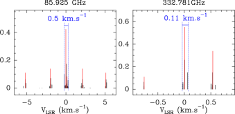
Figure 2: Line-strengths, normalized and centered on rest frequencies, for the 86 GHz and 333 GHz lines of o–NH₂D. In black, the spectroscopy accounts for the coupling with D while the spectroscopy obtained just accounting for N is shown in red.

5 Conclusion

We have observed the $1_{11}$-$1_{01}$ and $1_{01}$-$0_{00}$ lines of o/p-NH₂D towards the prestellar core H-MM1, and calculated the hyperfine patterns of the observed transitions. We found that when the hyperfine splitting induced by the D nucleus is neglected (as done in previous studies), the line analysis leads to inconsistent results pertaining the linewidths of the two transitions of o/p-NH₂D. For both spin isomers, the widths of the $1_{11}$-$1_{01}$ and $1_{01}$-$0_{00}$ lines differ by a factor of 1.6$\pm$0.3 if the D coupling is not taken into account. On the contrary, the new line list gives comparable linewidths for all the transitions. An error in the linewidth will be transferred to the column density estimate, and the effect is particularly pronounced for the $1_{11}$-$1_{01}$ lines of ortho and para-NH₂D at 86 and 110 GHz. In the case of H-MM1, the column density estimates derived from these lines with or without the hyperfine structure owing to D differ by a factor of $\sim$1.5.

111		101		p-NH2D		o–NH2D
F1	F	F1’	F’	$\nu$ (MHz)	Aul (s-1)	$\nu$ (MHz)	Aul (s-1)
0	1	1	0	110151.982	1.95 ( 6)	85924.691	9.23 ( 7)
0	1	1	2	110152.040	9.18 ( 6)	85924.749	4.35 ( 6)
0	1	1	1	110152.072	5.20 ( 6)	85924.781	2.46 ( 6)
0	1	2	2	110152.565	6.21 ( 8)	85925.273	2.93 ( 8)
0	1	2	1	110152.662	1.52 ( 7)	85925.370	7.17 ( 8)
2	1	1	0	110152.935	1.99 ( 6)	85925.644	9.43 ( 7)
2	2	1	2	110152.954	6.05 ( 7)	85925.662	2.87 ( 7)
2	3	1	2	110152.980	4.44 ( 6)	85925.688	2.10 ( 6)
2	2	1	1	110152.986	2.52 ( 6)	85925.694	1.20 ( 6)
2	1	1	2	110152.993	4.85 ( 8)	85925.702	2.30 ( 8)
2	1	1	1	110153.025	3.36 ( 6)	85925.734	1.59 ( 6)
2	2	2	2	110153.478	8.81 ( 6)	85926.186	4.18 ( 6)
0	1	0	1	110153.484	2.82 (10)	85926.191	1.33 (10)
2	3	2	2	110153.504	1.07 ( 6)	85926.212	5.09 ( 7)
2	1	2	2	110153.517	2.72 ( 6)	85926.225	1.29 ( 6)
1	1	1	0	110153.534	1.58 ( 6)	85926.243	7.47 ( 7)
2	2	2	3	110153.536	2.09 ( 6)	85926.244	9.92 ( 7)
2	3	2	3	110153.562	1.10 ( 5)	85926.270	5.23 ( 6)
1	2	1	2	110153.574	2.92 ( 6)	85926.282	1.38 ( 6)
2	2	2	1	110153.576	2.48 ( 6)	85926.284	1.18 ( 6)
1	0	1	1	110153.580	2.73 ( 6)	85926.288	1.30 ( 6)
1	1	1	2	110153.592	2.10 ( 6)	85926.301	9.96 ( 7)
1	2	1	1	110153.606	1.04 ( 6)	85926.314	4.91 ( 7)
2	1	2	1	110153.615	8.30 ( 6)	85926.323	3.94 ( 6)
1	1	1	1	110153.625	1.15 ( 6)	85926.333	5.42 ( 7)
1	2	2	2	110154.098	1.45 ( 6)	85926.806	6.87 ( 7)
1	1	2	2	110154.117	5.18 ( 6)	85926.825	2.46 ( 6)
1	2	2	3	110154.156	5.63 ( 6)	85926.864	2.67 ( 6)
1	0	2	1	110154.170	9.22 ( 6)	85926.877	4.37 ( 6)
1	2	2	1	110154.196	1.11 ( 7)	85926.904	5.25 ( 8)
1	1	2	1	110154.215	6.91 ( 7)	85926.922	3.28 ( 7)
2	2	0	1	110154.397	2.64 ( 8)	85927.104	1.25 ( 8)
2	1	0	1	110154.437	1.24 ( 7)	85927.143	5.85 ( 8)
1	0	0	1	110154.991	4.59 ( 6)	85927.698	2.18 ( 6)
1	2	0	1	110155.017	5.40 ( 6)	85927.724	2.56 ( 6)
1	1	0	1	110155.036	5.85 ( 6)	85927.743	2.77 ( 6)

Table 2: Line list of the 1₁₁-1₀₁ o/p-NH₂D transitions, with the hyperfine structure due to both the nitrogen and deuterium nuclei. The A_ul coefficients are given in the format $a(b)$ such that A_ul = $a\,10^{-b}$.

101		000		o-NH2D		p–NH2D
F1	F	F1’	F’	$\nu$ (MHz)	Aul (s-1)	$\nu$ (MHz)	Aul (s-1)
0	1	1	2	332780.875	4.68 ( 6)	332821.618	4.37 ( 6)
0	1	1	1	332780.875	2.26 ( 6)	332821.618	2.11 ( 6)
0	1	1	0	332780.875	1.20 ( 6)	332821.618	1.12 ( 6)
2	1	1	2	332781.695	3.14 ( 7)	332822.439	2.93 ( 7)
2	1	1	1	332781.695	4.54 ( 6)	332822.439	4.24 ( 6)
2	1	1	0	332781.695	3.29 ( 6)	332822.439	3.07 ( 6)
2	3	1	2	332781.735	8.14 ( 6)	332822.479	7.60 ( 6)
2	2	1	2	332781.793	1.59 ( 6)	332822.537	1.48 ( 6)
2	2	1	1	332781.793	6.56 ( 6)	332822.537	6.12 ( 6)
1	1	1	1	332782.285	1.35 ( 6)	332823.029	1.25 ( 6)
1	1	1	2	332782.285	3.15 ( 6)	332823.029	2.94 ( 6)
1	1	1	0	332782.285	3.65 ( 6)	332823.029	3.41 ( 6)
1	2	1	1	332782.317	1.59 ( 6)	332823.062	1.48 ( 6)
1	2	1	2	332782.317	6.56 ( 6)	332823.062	6.12 ( 6)
1	0	1	1	332782.375	8.14 ( 6)	332823.120	7.60 ( 6)

Table 3: Same as Table 2 but for the 1₀₁-0₀₀ o/p-NH₂D transitions.