Tight bounds of quantum speed limit for noisy dynamics
via maximal rotation angles

Abstract

The laws of quantum physics place a limit on the speed of computation. In particular, the evolution time of a system from an initial state to a final state cannot be arbitrarily short. Bounds on the speed of evolution for unitary dynamics have long been studied. A few bounds on the speed of evolution for noisy dynamics have also been obtained recently, which, however, are in general not tight. In this paper, we present a new framework for quantum speed limit concerning noisy dynamics. Within this framework we obtain the exact maximal rotation angle that noisy dynamics can achieve at any given time, which gives rise to a tight bound on the evolution time for noisy dynamics. The obtained bound clearly reveals that noisy dynamics are essentially different from unitary dynamics. Furthermore, we show that the orthogonalization time, which is the minimum time needed to evolve any state to its orthogonal state, is in general not applicable to noisy dynamics.

Zihao Hu, Lingna Wang, Hongzhen Chen, Haidong Yuan, Chi-Hang Fred Fung, Jing Liu and Zibo Miao

Zihao Hu
School of Mechanical Engineering and Automation,
Harbin Institute of Technology, Shenzhen, 518055, China;
Mechanical and Automation Engineering, The Chinese University of Hong Kong

Lingna Wang
Mechanical and Automation Engineering, The Chinese University of Hong Kong

Hongzhen Chen
Mechanical and Automation Engineering, The Chinese University of Hong Kong

Haidong Yuan
Mechanical and Automation Engineering, The Chinese University of Hong Kong

Chi-Hang Fred Fung
Canada Research Centre, Huawei Technologies Canada, Ontario, Canada

Jing Liu
National Precise Gravity Measurement Facility, MOE Key Laboratory of Fundamental Physical Quantities Measurement, School of Physics,
Huazhong University of Science and Technology, Wuhan 430074, China

Zibo Miao
School of Mechanical Engineering and Automation,
Harbin Institute of Technology, Shenzhen, 518055, China
E-mail: miaozibo@hit.edu.cn

1 Introduction

Quantum information processing may be regarded as the transformation of quantum states encoding the information to be processed or computed. The time for which the states transform dictates the speed of the quantum computation. Quantum physics imposes a limit on the transformation time. This quantum speed limit (QSL) [1] arises because the energy of the system and environment is finite and the system state may evolve according to slow dynamics. Over the period of time $t$, a quantum process may rotate an initial state by an angle $\theta$. In terms of QSL, the reverse question is asked. Namely, given a certain angle $\theta$, we ask what the minimum time $t$ is needed to rotate any state by the angle $\theta$.

The first major result of QSL, which was based on the uncertainty relation, was made by Mandelstam and Tamm [2] in 1945. Since then, there has been arising interets and development in the topic of SQL, including generalization to mixed states, Markovian and non-Markovian dynamics, closed and open quantum systems, different targets such as gauge invariant distances and Bloch angle, and many other applications such as optimal control and the the operational definition of QSL [38, 56, 55, 54, 53, 52, 37, 51, 50, 49, 36, 35, 48, 47, 34, 33, 32, 46, 45, 31, 44, 30, 43, 42, 29, 28, 7, 41, 40, 39, 63, 62, 61, 60, 59, 58, 57, 27, 26, 25, 24, 23, 22, 21, 20, 19, 18, 17, 16, 15, 14, 13, 12, 11, 10, 9, 8, 6, 5, 4, 3, 64]. While various results on unitary dynamics have come out (see e.g. [3, 7, 6, 4, 5, 9, 8, 10, 11, 12, 13, 14, 15, 16, 17, 18]), studies on noisy dynamics and open quantum systems have only been carried out recently [19, 20, 21, 22, 23, 24, 25, 26, 27, 28, 29, 30, 31, 32, 33, 34, 35, 36, 37, 38, 41, 40, 39].

In this paper, we present a new framework for QSL concerning noisy dynamics. Although previous studies mostly focus on the rotating speed of a given state under certain dynamics, here we study the maximal speed of evolution that the dynamics can generate on all quantum states, which requires an optimization over all states. The obtained speed of evolution represents the limit of quantum speed that the given dynamics can possibly induce on any quantum states, which is then a fundamental limit of the dynamics and can be used to provide bounds on the computation speed of a quantum device. While the QSL on a fixed state tells little about the ability of the dynamics with regard to rotation of the states in general, the maximal speed of evolution provides a way to gauge the dynamics.

Our framework is based on a method that gives the exact maximal rotation angle for certain given dynamics, which ensures that the bound is achievable. And the bound is obtained directly from the Kraus operators of the dynamics, allowing for the ease of computation. The obtained bound reveals that noisy dynamics are essentially different from unitary dynamics. In particular we show that the orthogonalization time, a concept commonly used in QSL, is in general not applicable to noisy dynamics.

Our framework builds on a distance measure on quantum channels [61] which will be briefly described in the following. For an $m\times m$ unitary matrix $U$, we denote by $e^{-\mbox{i}\theta_{j}}$ the eigenvalues of $U$, where $\theta_{j}\in(-\pi,\pi]$ for $1\leq j\leq m$ is also referred to as the eigen-angles of $U$. We define (see e.g. [57, 58, 59]) $\parallel U\parallel_{\max}=\max_{1\leq j\leq m}\mid\theta_{j}\mid,$ and $\parallel U\parallel_{g}$ as the minimum of $\parallel e^{i\gamma}U\parallel_{\max}$ over equivalent unitary operators with different global phases, i.e., $\parallel U\parallel_{g}=\min_{\gamma\in\mathbb{R}}\parallel e^{i\gamma}U\parallel_{\max}$. We then define

$$C_{\theta}(U)=\left\{\begin{array}[]{cc}\parallel U\parallel_{g},&if\parallel U\parallel_{g}\leq\frac{\pi}{2},\\ \frac{\pi}{2},&if\parallel U\parallel_{g}>\frac{\pi}{2}.\\ \end{array}\right.$$ (3)

Essentially $C_{\theta}(U)$ represents the maximal angle that $U$ can rotate a state away from itself [59, 61], i.e., $\cos[C_{\theta}(U)]=\min_{\rho}F_{B}(\rho,U\rho U^{\dagger}),$ where $F_{B}(\rho_{1},\rho_{2})$ is the fidelity between two states $F_{B}(\rho_{1},\rho_{2})=\operatorname{tr}\sqrt{\rho_{1}^{\frac{1}{2}}\rho_{2}\rho_{1}^{\frac{1}{2}}}.$

If $\theta_{\max}=\theta_{1}\geq\theta_{2}\geq\cdots\geq\theta_{m}=\theta_{\min}$ are arranged in decreasing order, then $C_{\theta}(U)=\frac{\theta_{\max}-\theta_{\min}}{2}$ when $\theta_{\max}-\theta_{\min}\leq\pi$ [59]. A metric on unitary operators can be induced by $C_{\theta}(U)$ as $d(U_{1},U_{2})=C_{\theta}(U_{1}^{\dagger}U_{2});$ $d(U_{1},U_{2})$ represents the maximal angle $U_{1}$ and $U_{2}$ can generate on the same input state, with $\cos d(U_{1},U_{2})=\min_{\rho}F_{B}(U_{1}\rho U_{1}^{\dagger},U_{2}\rho U_{2}^{\dagger})$ [61].

This metric can be generalized to noisy dynamics as $d(K_{1},K_{2})=\min_{U_{ES_{2}}}d(U_{ES_{1}},U_{ES_{2}}),$ where $U_{ES_{1}}$ and $U_{ES_{2}}$ are unitary extensions of $K_{1}$ and $K_{2}$ respectively. And $d(K_{1},K_{2})$ can be computed from the Kraus operators of $K_{1}$ and $K_{2}$ as $d(K_{1},K_{2})=\arccos\max_{\|W\|\leq 1}\frac{1}{2}\lambda_{\min}(K_{W}+K^{\dagger}_{W})$[61], where $\lambda_{\min}(K_{W}+K^{\dagger}_{W})$ denotes the minimum eigenvalue of $K_{W}+K^{\dagger}_{W}$ with $K_{W}=\sum_{j=1}^{D}\sum_{i=1}^{D}w_{ij}F_{1i}^{\dagger}F_{2j}$. Here $F_{1i}$ and $F_{2j}$, $1\leq i,j\leq D$, denote the Kraus operators of $K_{1}$ and $K_{2}$ respectively, $w_{ij}$ denotes the $ij$-th entry of a $D\times D$ matrix $W$ with $\|W\|\leq 1$($\|\cdot\|$ is the operator norm which is equal to the maximum singular value). $d(K_{1},K_{2})$ represents the maximal angle that $K_{1}\otimes I_{A}$ and $K_{2}\otimes I_{A}$ can generate with respect to the same input state; $\cos d(K_{1},K_{2})=\min_{\rho_{SA}}F_{B}[K_{1}\otimes I_{A}(\rho_{SA}),K_{2}\otimes I_{A}(\rho_{SA})]$, where $\rho_{SA}$ is a state of the composite systems consisting of the target and ancilla, with $I_{A}$ denoting the identity operator defined in the ancillary system [61]. Furthermore this distance can be efficiently calculated via semi-definite programming as $\max_{\|W\|\leq 1}\frac{1}{2}\lambda_{\min}(K_{W}+K^{\dagger}_{W})=$

$$\begin{aligned} &\max\qquad\frac{1}{2}t\\ s.t.\qquad&\left(\begin{array}[]{cc}I&W^{\dagger}\\ W&I\\ \end{array}\right)\succeq 0,\\ &K_{W}+K^{\dagger}_{W}-tI\succeq 0.\end{aligned}$$ (4)

And the dual semi-definite programming provides a way to find the optimal state [62]:
$\max_{\|W\|\leq 1}\frac{1}{2}\lambda_{\min}(K_{W}+K^{\dagger}_{W})=$

$$\begin{aligned} \min\qquad&\frac{1}{2}\operatorname{tr}(P)+\frac{1}{2}\operatorname{tr}(Q)\\ s.t.\qquad&\left(\begin{array}[]{cc}P&M^{\dagger}(\rho_{S})\\ M(\rho_{S})&Q\\ \end{array}\right)\succeq 0,\\ &\rho_{S}\succeq 0,\\ &\operatorname{tr}(\rho_{S})=1,\end{aligned}$$ (5)

where $P,Q$ are Hermitian matrices and $M(\rho_{S})$ is a $D\times D$ matrix with its $ij$-th entry equaling $\operatorname{tr}(\rho_{S}F_{1i}^{\dagger}F_{2j})$. The optimal state is any pure state $\rho_{SA}$ with $\operatorname{tr}_{A}({\rho_{SA}})=\rho_{S}$, where $\rho_{S}$ is obtained from the above semi-definite programming [62].

The metric can be used to obtain a saturable bound for QSL. More precisely, the dynamics $K_{t}(\rho)=\sum_{i}F_{i}(t)\rho F_{i}^{\dagger}(t)$, suppose it takes $t$ units of time for the dynamics to rotate a state, possibly entangled with an ancillary system, with an angle $\theta$. Then $\theta=\arccos F_{B}[\rho_{SA},K_{t}\otimes I_{A}(\rho_{SA})]\leq d(I,K_{t})$, and thus a lower bound on the minimum time can be obtained by this inequality where the equality can be saturated when $\rho_{SA}$ takes the optimal input state. When $\rho_{SA}$ is restricted to separable states, the maximal rotation speed is reduced to the case without an ancillary system, which is in general slower. $d(I,K_{t})$ thus provides a limit on the maximal angle that the given dynamics can generate on any state at the time $t$.

First of all, for unitary dynamics $U_{t}=e^{-\mbox{i}Ht}$, suppose it takes $t$ units of time to rotate a state $\rho$ with the angle $\theta\in[0,\frac{\pi}{2}]$. Then $\theta\leq d(I,U_{t})=\frac{(E_{\max}-E_{\min})t}{2},$ where $E_{\max}$($E_{\min}$) denotes the maximum(minimum) eigenvalue of $H$. The minimum time needed to rotate a state away with the angle $\theta$ is then bounded by $t\geq\frac{2\theta}{E_{\max}-E_{\min}}$. This recovers previous results on the quantum speed limit for unitary dynamics [8]. This bound is also known to be saturable with the input state $|\varphi\rangle=\frac{1}{\sqrt{2}}(|E_{\max}\rangle+e^{\mbox{i}\phi}|E_{\min})$, which can always be rotated to an orthogonal state at the time $t=\frac{\pi}{E_{\max}-E_{\min}}$.

Here $E_{\max}-E_{\min}$ can be seen as the energy scale of the system, and thus $d(I,U_{t})$ is proportional to the multiplication of the energy scale and time. The maximal angle that can be rotated is thus proportional to the time-energy cost of the dynamics [57, 58, 59, 60]. For noisy dynamics, as $d(I,K_{t})=\min_{U_{ES_{t}}}(I_{ES},U_{ES_{t}})$ where $U_{ES_{t}}$ is the unitary extension of $K_{t}$, the maximal angle is proportional to the minimum time-energy cost over all unitary extensions of the noisy dynamics [57, 58, 59, 60].

In the following part of this paper, we will focus on the analysis of QSL concerning noisy dynamics.

2 QSL for single systems

In this section, we will be concerned with the analysis of QSL, characterized by the maximal rotation angle, under noisy dynamics for single systems.

Dynamics with amplitude damping. Consider the Markovian dynamics with amplitude damping $K_{t}(\rho)=F_{11}(t)\rho F_{11}^{\dagger}(t)+F_{12}(t)\rho F_{12}^{\dagger}(t)$, where the Kraus operators $F_{11}(t)=\begin{bmatrix}1&0\\ 0&\sqrt{P(t)}\end{bmatrix}$, $F_{12}(t)=\begin{bmatrix}0&\sqrt{1-P(t)}\\ 0&0\end{bmatrix}$. Here the time-varying element $P(t)=e^{-\gamma t}$ with $\gamma$ being the decay rate. Suppose it takes $t$ units of time for the dynamics to rotate a state $\rho_{SA}$ with the angle $\theta\in[0,\frac{\pi}{2}]$. The density operator $\rho_{SA}$ represents the quantum state of the target system and the ancilla, and then one can have that $\theta=\arccos F_{B}[\rho_{SA},K_{t}\otimes I_{A}(\rho_{SA})]\leq\arccos\min_{\rho_{SA}}F_{B}[\rho_{SA},K_{t}\otimes I_{A}(\rho_{SA})]=d(I,K_{t})$.

One can have that $\cos d(I,K_{t})=\max_{\|W\|\leq 1}\frac{1}{2}\lambda_{\min}(K_{W}+K_{W}^{\dagger})$, where $K_{W}=\sum_{ij}w_{ij}F_{0i}^{\dagger}F_{1j}$. with $F_{01}=I$ and $F_{02}=\mathbf{0}$ being the Kraus operators for the identity operator (where a zero operator has been added). Here $w_{ij}$ is the $ij$-th entry of the $2\times 2$ matrix $W$ satisfying $\|W\|\leq 1$. Then $K_{W}+K_{W}^{\dagger}=\begin{bmatrix}a&c\\ c^{*}&b\end{bmatrix}$, with $a=2\mathbb{R}(w_{11})$, $b=2\mathbb{R}(w_{11})\sqrt{P(t)}$, and $c=w_{12}\sqrt{1-P(t)}$ ($\mathbb{R}(w_{11})$ denotes the real part of $w_{11}$). The minimum eigenvalue of $K_{W}+K_{W}^{\dagger}$ can thus be given by $\lambda_{\min}(K_{W}+K_{W}^{\dagger})=\frac{a+b-\sqrt{(a-b)^{2}+4|c|^{2}}}{2}$. In order to maximize the minimum eigenvalue, $c$ should be made $0$. Or rather say, $w_{12}$ is chosen to be $0$, and then $\lambda_{\min}(K_{W}+K_{W}^{\dagger})=b=2\mathbb{R}(w_{11})\sqrt{P(t)}$ reaching the maximum value when $w_{11}=1$. Therefore, $\cos d(I,K_{t})=\max_{\|W\|\leq 1}\frac{1}{2}\lambda_{\min}(K_{W}+K_{W}^{\dagger})=\sqrt{P(t)}$. As $\theta\leq d(I,K_{t})$, we have that $\cos\theta\geq\cos d(I,K_{t})=\sqrt{P(t)}$, which gives $t\geq\frac{2}{\gamma}\ln\sec\theta$. This provides a lower bound for the minimum time needed to rotate any state with the angle $\theta$, and it is consistent with the previous results (see e.g. [19]). Please note that in this scenario in order to rotate a state to its orthogonal state, infinite time is needed as $\ln\sec\frac{\pi}{2}\rightarrow\infty$. In fact, this corresponds to the case where the initial state is the excited state $|1\rangle$ and it only decays completely to the ground state $|0\rangle$ within infinite amount of time.

For non-Markovian dynamics, due to strong couplings to the environment, the decay rate $\gamma_{nM}(t)$, which is usually time-dependent, can be bigger than the decay rate in the Markovian regime [21]. Therefore, in such a case $P(t)=e^{-\int_{0}^{t}\gamma_{nM}(\tau)d\tau}$ where $\int_{0}^{t}\gamma_{nM}(\tau)d\tau$ is usually bigger than $\gamma t$ in the Markovian regime, thus for the same time duration the maximal angle $d(I,K_{t})=\arccos\sqrt{P(t)}$ can be bigger in the non-Markovian regime than that in the Markovian regime. This was explored in previous studies showing that non-Markovian dynamics can speed up the rotation [21]. Please note that even in the non-Markovian regime, as long as $\gamma_{nM}(t)$ is finite, it always needs infinite amount of time for $P(t)$ to reach $0$. And thus it always needs infinite amount of time to achieve a $\pi/2$-rotation.

Dynamics with dephasing noises. Let $K_{t}(\rho)=F_{11}(t)\rho F_{11}^{\dagger}(t)+F_{12}(t)\rho F_{12}^{\dagger}(t)$ describe the dynamics in the presence of dephasing noises, with the Kraus operators $F_{11}(t)=\sqrt{\frac{1+P(t)}{2}}\begin{bmatrix}e^{-\mbox{i}\omega t/2}&0\\ 0&e^{\mbox{i}\omega t/2}\end{bmatrix}$ and $F_{12}(t)=\sqrt{\frac{1-P(t)}{2}}\begin{bmatrix}e^{-\mbox{i}\omega t/2}&0\\ 0&-e^{\mbox{i}\omega t/2}\end{bmatrix}$. Here $P(t)=e^{-\gamma t}$ and $\gamma$ denotes the dephasing rate. We similarly suppose it takes $t$ units of time for the dynamics to rotate the quantum state $\rho_{SA}$ with the angle $\theta\in[0,\frac{\pi}{2}]$, and thus $\theta\leq d(I,K_{t})$. In this scenario, we have that $K_{W}+K_{W}^{\dagger}=\begin{bmatrix}a&0\\ 0&b\end{bmatrix}$ with $a=2\mathbb{R}\left(\sqrt{\frac{1+P(t)}{2}}w_{11}e^{-\mbox{i}\omega t/2}+\sqrt{\frac{1-P(t)}{2}}w_{12}e^{-\mbox{i}\omega t/2}\right)$, $b=2\mathbb{R}\left(\sqrt{\frac{1+P(t)}{2}}w_{11}e^{\mbox{i}\omega t/2}-\sqrt{\frac{1-P(t)}{2}}w_{12}e^{\mbox{i}\omega t/2}\right)$. By using $|w_{11}|^{2}+|w_{12}|^{2}\leq 1$ for any $\|W\|\leq 1$ together with the Cauchy-Schwarz inequality, one can obtain that

$$\lambda_{\min}(K_{W}+K_{W}^{\dagger})\leq \frac{1}{2}\operatorname{tr}(K_{W}+K_{W}^{\dagger})$$

$$= 2\mathbb{R}\left(\sqrt{\frac{1+P(t)}{2}}w_{11}\cos(\omega t/2)-\mbox{i}\sqrt{\frac{1-P(t)}{2}}w_{12}\sin(\omega t/2)\right)$$

$$\leq 2[|\sqrt{\frac{1+P(t)}{2}}w_{11}\cos(\omega t/2)|+|\sqrt{\frac{1-P(t)}{2}}w_{12}\sin(\omega t/2)|$$

$$\leq 2\sqrt{\frac{1+P(t)}{2}\cos^{2}(\omega t/2)+\frac{1-P(t)}{2}\sin^{2}(\omega t/2)}\sqrt{|w_{11}|^{2}+|w_{12}|^{2}}$$

$$\leq 2\sqrt{\frac{1+P(t)\cos(\omega t)}{2}}.$$

It is not difficult to verify that the equality is saturated when $w_{11}=\frac{\sqrt{1+P(t)}\cos(\omega t/2)}{\sqrt{1+P(t)\cos(\omega t)}},w_{12}=\frac{\mbox{i}\sqrt{1-P(t)}\sin(\omega t/2)}{\sqrt{1+P(t)\cos(\omega t)}}.$ It can then be concluded that $\cos d(I,K_{t})=\sqrt{\frac{1+P(t)\cos(\omega t)}{2}}.$ Then from $\cos\theta\geq\cos d(I,K_{t})$, the minimum time needed to rotate a state with the angle $\theta$ can be obtained,

Figure 1: The maximal angles that can be rotated at different values of the time $t$ in the presence of dephasing noises, with $\gamma=0.1$ and $\omega=1$.

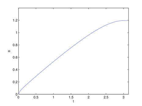
which is illustrated in Fig.1.

It is worth noting that $\cos d(I,K_{t})=\sqrt{\frac{1+e^{-\gamma t}\cos(\omega t)}{2}}>0$ for $P(t)=e^{-\gamma t}$ as long as $\gamma>0$. Hence $d(I,K_{t})<\pi/2$; namely the dynamics cannot rotate any state to its orthogonal state. This is a much stronger statement than the previous result in [19] where it was stated that only when $\frac{\omega}{\gamma}>r_{crit}\approx 2.6$ the dynamics could not rotate any state to its orthogonal state. Such difference arises as the previous bound is obtained from the integration of the quantum Fisher metric along the path $\rho_{t}=K_{t}\otimes I_{A}(\rho_{SA})$. Such a path is fixed by the dynamics which is usually not the geodesic between the initial state and the final state indeed. Consequently, the integration of the quantum Fisher metric along the path is in general bigger than the actual distance between the initial state and the final state. This in turn leads to a looser bound and inaccurate classification for noisy dynamics. The bound obtained in [20] for dynamics with dephasing noises is also not tight, which resulted in a finite orthogonalization time. By contrast, the bound obtained here is tight and can be saturated with the input state $|+\rangle=\frac{|0\rangle+|1\rangle}{\sqrt{2}}$. In addition, an ancillary system is not needed to saturate the bound we have obtained in the presence of dephasing noises.

Generic noisy dynamics. In this part we will show that generic noisy dynamics cannot rotate any state to its orthogonal state. In particular, for the given dynamics $K_{t}(\rho)=\sum_{i=1}^{D}F_{i}(t)\rho F_{i}^{\dagger}(t)$, we will show that if $I\in\{F_{1}(t),F_{2}(t),\cdots,F_{D}(t)\}$, then $K_{t}$ cannot rotate any state to its orthogonal state. Or Equivalently, if the identity operator belongs to the space spanned by the Kraus operators then $d(I,K_{t})$ is always smaller than $\frac{\pi}{2}$. The reason lies in the fact that if $I\in\{F_{1}(t),F_{2}(t),\cdots,F_{D}(t)\}$, then there exists $w_{1i}$ such that $I=\sum_{i=1}^{D}w_{1i}F_{i}(t)$. Now let $\alpha=1/\sqrt{\sum_{i=1}^{D}|w_{1i}|^{2}}>0$, then $\alpha I=\sum_{i=1}^{D}w^{\prime}_{1i}F_{i}(t)$ with $w^{\prime}_{1i}=\alpha w_{1i}$. Define $W^{\prime}$ as a $D\times D$ matrix with the entries of the first row equal to $w^{\prime}_{1i}$ and other entries equal to $0$. It is then obvious that $\|W^{\prime}\|=1$, and thus

$$\begin{aligned} \cos d(I,K_{t})&=\max_{\|W\|\leq 1}\frac{1}{2}\lambda_{\min}(K_{W}+K_{W}^{\dagger})\\ &\geq\frac{1}{2}\lambda_{\min}(K_{W^{\prime}}+K_{W^{\prime}}^{\dagger})\\ &=\frac{1}{2}\lambda_{\min}[\sum_{i=1}^{D}w^{\prime}_{1i}F_{i}(t)+(\sum_{i=1}^{D}w^{\prime}_{1i}F_{i}(t))^{\dagger}]\\ &=\alpha>0.\end{aligned}$$ (6)

Hence $d(I,K_{t})\leq\arccos\alpha<\pi/2$. Namely, the dynamics cannot rotate any state to its orthogonal state.

For example, in the presence of dephasing noises, we have $F_{11}(t)=\sqrt{\frac{1+P(t)}{2}}\begin{bmatrix}e^{-\mbox{i}\omega t/2}&0\\ 0&e^{\mbox{i}\omega t/2}\end{bmatrix}$ and $F_{12}(t)=\sqrt{\frac{1-P(t)}{2}}\begin{bmatrix}e^{-\mbox{i}\omega t/2}&0\\ 0&-e^{\mbox{i}\omega t/2}\end{bmatrix}$, with $P(t)=e^{-\gamma t}$ and $\gamma$ being the dephasing rate. In this case $I=\sqrt{\frac{2}{1+P(t)}}\cos(\omega t/2)F_{11}(t)+\mbox{i}\sqrt{\frac{2}{1-P(t)}}\sin(\omega t/2)F_{12}(t),$ and then

$$\begin{aligned} \alpha&=\frac{1}{\sqrt{\frac{2}{1+P(t)}\cos^{2}(\omega t/2)+\frac{2}{1-P(t)}\sin^{2}(\omega t/2)}}\\ &=\frac{\sqrt{1-P^{2}(t)}}{\sqrt{2-2P(t)\cos(\omega t)}},\end{aligned}$$ (7)

which is positive for any $P(t)<1$. Hence, in the presence of dephasing noises, $d(I,K_{t})\leq\arccos\alpha<\pi/2$.

This fact can also be easily seen from the equivalent representations of Kraus operators. More precisely, when $I\in\{F_{1}(t),F_{2}(t),\cdots,F_{D}(t)\}$, there exists an equivalent representation of Kraus operators such that $\alpha I$ is one of them. Then the fidelity between the initial state and final state will be at least $\alpha$, and thus such dynamics cannot rotate any state to its orthogonal state. The bound proposed by us can not only reflect this fact, but can also provide tighter bound by exploring different choices of $W$. Taking the dynamics with dephasing noises for example, the choice of $W=\begin{bmatrix}\frac{\sqrt{1+P(t)}\cos(\omega t/2)}{\sqrt{1+P(t)\cos(\omega t)}}&\frac{\mbox{i}\sqrt{1-P(t)}\sin(\omega t/2)}{\sqrt{1+P(t)\cos(\omega t)}}\\ 0&0\end{bmatrix}$ can lead to the tight bound. In addition, it is not difficult to observe that if the span of Kraus operators contains any matrix $M$ such that $\lambda_{\min}(M+M^{\dagger})>0$, the above argument holds. And thus the dynamics cannot rotate any state to its orthogonal state. Taking the dynamics with amplitude damping for example, the span of the associated Kraus operators contains $M=\begin{bmatrix}1&0\\ 0&\sqrt{P(t)}\end{bmatrix}$, which satisfies the condition $\lambda_{\min}(M+M^{\dagger})=2\sqrt{P(t)}>0$ except for $P(\infty)=0$.

One immediate implication is that all dynamics with the associated Kraus operators spanning the whole space(or equivalently the number of linearly independent Kraus operators is $d=n^{2}$ where $n$ denotes the dimension of the quantum system) cannot rotate any state to its orthogonal state. Such dynamics are indeed generic among all completely positive trace preserving maps, therefore generic noisy dynamics cannot rotate any state to its orthogonal state.

Figure 2: The maximal angles that can be rotated in composite systems in the presence of dephasing noises, with the lower and upper bounds at different values of $\frac{\omega}{\gamma}$ plotted. These curves are obtained by figuring out the optimal time spot $t$ that gives the maximal angle for the separable state, $d(I^{\otimes^{N}},K_{t}^{\otimes N})$ and $\arccos(\alpha^{N})$ respectively with $N=5$. It can be seen that $\max_{t}\theta_{sep}$ and $\max_{t}\arccos(\alpha^{N})$ provides tight bounds for $\max_{t}d(I^{\otimes^{N}},K_{t}^{\otimes N})$. The maximal angle that can be achieved with the GHZ state is also plotted for comparison.

3 QSL for composite systems

Given the noisy dynamics $K_{t}(\rho)=\sum_{i=1}^{D}F_{i}(t)\rho F^{\dagger}_{i}(t)$, we now suppose there are $N$ number of such dynamics, denoted by $K_{t}^{\otimes^{N}}$, acting independently on a composite system. Similar to the discussions in Section 2, if $I\in\{F_{1}(t),F_{2}(t),\cdots,F_{D}(t)\}$, then there exists $w_{1i}$ such that $I=\sum_{i=1}^{D}w_{1i}F_{i}(t)$. Let $\alpha=1/\sqrt{\sum_{i=1}^{D}|w_{1i}|^{2}}>0$, then $\alpha I=\sum_{i=1}^{D}w^{\prime}_{1i}F_{i}(t)$ with $w^{\prime}_{1i}=\alpha w_{1i}$. Here $W^{\prime}$ is a $D\times D$ matrix defined with the entries of the first row equal to $w^{\prime}_{1i}$ and other entries equal to $0$. Now one representation of the Kraus operators for $K_{t}^{\otimes^{N}}$ can be written as $\tilde{F}_{i_{1},i_{2},\cdots,i_{N}}(t)=F_{i_{1}}(t)\otimes F_{i_{2}}(t)\otimes\cdots\otimes F_{i_{N}}(t)$. Let $\tilde{W}=W^{\prime\otimes N}$, then $K^{\otimes N}_{\tilde{W}}=(K_{W^{\prime}})^{\otimes^{N}}=\alpha^{N}I^{\otimes^{N}}$. One can thus have that

$$\begin{aligned} \cos d(I^{\otimes^{N}},K_{t}^{\otimes N})&=\max_{\|W\|\leq 1}\frac{1}{2}\lambda_{\min}(K^{\otimes N}_{W}+(K^{\otimes N}_{W})^{\dagger})\\ &\geq\frac{1}{2}\lambda_{\min}(K^{\otimes N}_{\tilde{W}}+(K^{\otimes N}_{\tilde{W}})^{\dagger})\\ &=\lambda_{\min}(\alpha^{N}I^{\otimes^{N}})\\ &=\alpha^{N}>0,\end{aligned}$$

which implies $d(I^{\otimes^{N}},K_{t}^{\otimes N})\leq\arccos(\alpha^{N})<\pi/2$. It can then be concluded that in this case any state of the composite system cannot be rotated to its orthogonal state.

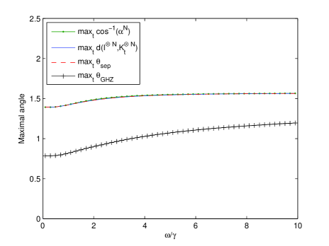
In fact, in the presence of dephasing noises, by substituting the value of $\alpha$ in Eq.(7), one can obtain an upper bound for $d(I^{\otimes^{N}},K_{t}^{\otimes N})$ straightforwardly. A lower bound for $d(I^{\otimes^{N}},K_{t}^{\otimes N})$ can also be obtained by taking the input state as the separable state $|+\cdots+\rangle$, where $|+\rangle=(|0\rangle+|1\rangle)/\sqrt{2}$. It is then not difficult to calculate the rotated angle with respect to this separable state, which is $\theta_{sep}=\arccos(\beta^{N})$ with $\beta=\sqrt{\frac{1+e^{-\gamma t}\cos(\omega t)}{2}}$, and thus $\arccos(\beta^{N})\leq d(I^{\otimes^{N}},K_{t}^{\otimes N})\leq\arccos(\alpha^{N}).$ Then the inequality $\max_{t}\arccos(\beta^{N})\leq\max_{t}d(I^{\otimes^{N}},K_{t}^{\otimes N})\leq\max_{t}\arccos(\alpha^{N})$ bounds the maximal angle that can be rotated for composite systems. In Fig.2, we plot these bounds and the exact maximal angle for composite systems in the presence of dephasing noises. It can be seen that these bounds are quite tight.

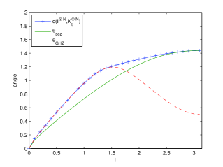
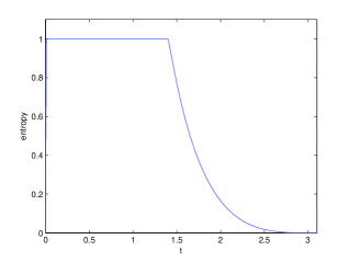
On the other hand, for composite systems, the GHZ state (i.e.,$(|0\cdots 0\rangle+|1\cdots 1\rangle)/\sqrt{2}$) is usually used as a benchmark for the QSL [19, 20]. The rotation angle on the GHZ state can be explicitly computed as $\cos\theta_{GHZ}=\sqrt{\frac{1+e^{-N\gamma t}\cos(N\omega t)}{2}}.$ It can be seen from Fig. 3(a) that for small values of $t$ (i.e., when the noise influence is still not strong), the GHZ state can help achieve the maximal speed of evolution. However, for big values of $t$, the GHZ state is no longer the optimal state that achieves the maximal angle $d(I^{\otimes^{N}},K_{t}^{\otimes N})$. More precisely, the GHZ state can be even worse than the separable state. This can be clearly observed in Fig. 3(b), where we quantify the entanglement for the optimal state that saturates $d(I^{\otimes^{2}},K_{t}^{\otimes 2})$.

The maximally entangled state is only optimal when $t$ is under the threshold (e.g. $t<1.5$). When $t$ is beyond the threshold, the optimal state that achieves the maximal rotated angle gradually changes from the maximally entangled state to the separable state. Moreover, Fig. 2 shows that the maximal angle on the GHZ state is far smaller than the maximal angle on the separable state. This is because the maximal angle on the GHZ state actually does not change with $N$ (it only shortens the optimal time consumed to obtain the maximal angle by $N$ times). That is to say, $\max_{t}\theta_{GHZ}=\max_{t}\arccos\beta$ with $\beta=\sqrt{\frac{1+e^{-\gamma t}\cos(\omega t)}{2}}$, while $\max_{t}\theta_{sep}=\max_{t}\arccos(\beta^{N})$ increases with $N$. From another perspective, if we take the rotated angle as the degenerate effect under noisy dynamics, it indicates that although the GHZ state deteriorates fast in the presence of dephasing noises in a short period of time, in the long run the entanglement in the GHZ state mitigates the maximal degeneration.

(a) Rotation angles on the GHZ and separable states respectively, compared with the maximal angles.

(b) Quantified entanglement of the optimal input state which achieves the maximal rotated angle.

Figure 3: Understanding QSL under the noisy dynamics for composite systems in the presence dephasing noises with the parameters chosen as $\gamma=0.1,\omega=1,N=2$.

4 Conclusions and future work

We provide a new framework to calculate the exact maximal rotation angles for any noisy dynamics within a given evolution time. Namely, tight bounds have been obtained for QSL under noisy dynamics. The maximal rotation angles as well as the corresponding bounds given in this paper clearly show that the commonly used concept for QSL, i.e. the orthogonalization time, is in general not applicable to noisy dynamics. It is also shown that although maximally entangled states, such as the GHZ state, evolve faster in a short period of time, they are not the optimal states giving rise to the maximal rotation angles under noisy dynamics in the long run.

Furthermore, our work has implications to quantum computing since the state transformation time bounds the speed of computation. One the other hand, the amount of state degradation is bounded by the storage time, which thus leads to better understanding of quantum memory.

Conflict of Interest

The authors declare no conflict of interest.

References

• [1] S. Lloyd, Nature (London) 406, 1047 (2000).
• [2] L. Mandelstam and I. G. Tamm, J. Phys. (Moscow) 9, 249 (1945)
• [3] N. Margolus and L. B. Levitin, Physica D 120, 188 (1998).
• [4] H. F. Chau, Phys. Rev. A 81, 062133 (2010).
• [5] P. J. Jones and P. Kok, Phys. Rev. A 82, 022107 (2010).
• [6] V. Giovannetti, S. Lloyd, and L. Maccone, Phys. Rev. A 67, 052109 (2003).
• [7] V. Giovannetti, S. Lloyd, and L. Maccone, J. Opt. B 6, S807 (2004).
• [8] D. C. Brody, J. Phys. A: Math. Gen. 36, 5587Β¨C5593, (2003).
• [9] L. B. Levitin and T. Toffoli, Fundamental Limit on the Rate of Quantum Dynamics: The Unified Bound Is Tight, Phys. Rev. Lett. 103, 160502 (2009).
• [10] T. Caneva, M. Murphy, T. Calarco, R. Fazio, S. Montangero, V. Giovannetti, and G. E. Santoro, Phys. Rev. Lett. 103, 240501 (2009).
• [11] S. Luo, Physica D 189, 1 (2004).
• [12] S. Luo, J. Phys. A 38, 2991 (2005).
• [13] S. Fu, N. Li, and S. Luo, Commun. Theor. Phys. 54, 661 (2010).
• [14] L. Vaidman, Am. J. Phys., 60, pp. 182-183 (1992).
• [15] V. Giovannetti, S. Lloyd, and L. Maccone, Europhys. Lett., 62 (5), pp. 615-621 (2003).
• [16] J. Batle, M. Casas, A. Plastino, and A. R. Plastino, Phys. Rev. A. 72, 032337 (2005).
• [17] A. BorrΓ‘s, M. Casas, A. R. Plastino, and A. Plastino, Phys. Rev. A. 74, 022326 (2006).
• [18] J. Kupferman and B. Reznik, Phys. Rev. A. 78, 042305 (2008).
• [19] M. M. Taddei, B. M. Escher, L. Davidovich, and R. L. de Matos Filho, Phys. Rev. Lett. 110, 050402 (2013).
• [20] A. del Campo, I. L. Egusquiza, M. B. Plenio, and S. F. Huelga Phys. Rev. Lett. 110, 050403 (2013).
• [21] S. Deffner and E. Lutz, Quantum Speed Limit for Non-Markovian Dynamics, Phys. Rev. Lett. 111, 010402 (2013).
• [22] C. Liu, Z. Xu, and S. Zhu, Phys. Rev. A. 91, 022102 (2015).
• [23] Y.-J. Zhang, W. Han, Y.-J. Xia, J.-P. Cao, and H. Fan, Classical-driving-assisted quantum speed-up, Phys. Rev. A. 91, 032112 (2015).
• [24] Y.-J. Zhang, W. Han, Y.-J. Xia, J.-P. Cao, and H. Fan, Sci. Rep. 4, 4890 (2014).
• [25] S.Morley-Short, L. Rosenfeld, and P. Kok, Phys. Rev. A. 90, 062116 (2014).
• [26] Z.-Y. Xu, S. Luo, W. L. Yang, C. Liu, and S. Zhu, Phys. Rev. A 89, 012307 (2014).
• [27] Z.-Y. Xu and S.-Q. Zhu, Chin. Phys. Lett. 31, 020301 (2014).
• [28] Z. Sun, J. Liu, J. Ma, and X. Wang, Sci. Rep. 5, 8444 (2015).
• [29] I. Marvian, and D. A. Lidar, Phys. Rev. Lett. 115, 210402 (2015).
• [30] S.-X. Wu, and C.-S. Yu, Phys. Rev. A 98, 042132 (2018).
• [31] F. Campaioli, F. A. Pollock, and K. Modi, Quantum 3, 168 (2019).
• [32] D. P. Pires, M. Cianciaruso, L. C. CΓ©leri, G. Adesso, and D. O. Soares-Pinto, Phys. Rev. X 6, 021031 (2016).
• [33] A. Chenu, M. Beau, J. Cao, and A. del Campo, Phys. Rev. Lett. 118, 140403 (2017).
• [34] M. Beau, and A. del Campo, Phys. Rev. Lett. 119, 010403 (2017).
• [35] S. Deffner, and S. Campbell, J. Phys. A: Math. Theor. 50, 453001 (2017).
• [36] M. Beau, J. Kiukas, I. L. Egusquiza, and A. del Campo, Phys. Rev. Lett. 119, 130401 (2017).
• [37] D. Girolami, Phys. Rev. Lett. 122, 010505 (2019).
• [38] L. P. Garcia-Pintos, S. B. Nicholson, J. R. Green, A. del Campo, and A. V. Gorshkov, Phys. Rev. X 12, 011038 (2022).
• [39] Y. Shao, B. Liu, M. Zhang, H. Yuan, and J. Liu, Phys. Rev. Research 2, 023299 (2020).
• [40] J. Liu, Z. Miao, L. Fu, and X. Wang, Phys. Rev. A 104, 052432 (2021).
• [41] M. Zhang, H.-M. Yu, and J. Liu, npj Quantum Inf. 9, 97 (2023).
• [42] K. Funo et al, Phys. Rev. Lett. 118, 100602 (2017).
• [43] B. Shanahan, A. Chenu, N. Margolus and A. del Campo, Phys. Rev. Lett. 120, 070401 (2018).
• [44] F. Campaioli, F. A. Pollock, F. C. Binder and K. Modi, Phys. Rev. Lett. 120, 060409 (2018).
• [45] S. Sun, and Y. Zheng, Phys. Rev. Lett. 123, 180403 (2019).
• [46] S. Sun, Y. Peng, X. Hu and Y. Zheng, Phys. Rev. Lett. 127, 100404 (2021).
• [47] M. Bukov, D. Sels, and A. Polkovnikov, Phys. Rev. X 9, 011034 (2019).
• [48] G. C. Hegerfeldt, Phys. Rev. Lett 111, 260501 (2013).
• [49] S. Campbell, and S. Deffner, Phys. Rev. Lett. 118, 100601 (2017).
• [50] X. Cai, and Y. Zheng, Phys. Rev. A 95, 052104 (2017).
• [51] M. Okuyama, and M. Ohzeki, Phys. Rev. Lett. 120, 070402 (2018).
• [52] X. Hu, S. Sun, and Y. Zheng, Phys. Rev. A 101, 042107 (2020).
• [53] S. Becker, N. Datta, L. Lami, and C. RouzΓ©, Phys. Rev. Lett. 126, 190504 (2021).
• [54] G. Ness et al, Sci. Adv. 7, eabj9119 (2021).
• [55] A. del Campo, Phys. Rev. Lett. 126, 180603 (2021).
• [56] G. Ness, A. Alberti, and Y. Sagi, Phys. Rev. Lett. 129, 140403 (2022).
• [57] H. F. Chau, Quant. Inf. Compu. 11, 0721 (2011).
• [58] C.-H. F. Fung, and H. F. Chau, Phys. Rev. A 88, 012307 (2013).
• [59] C.-H. F. Fung, and H. F. Chau, Phys. Rev. A 90, 022333 (2014).
• [60] C.-H. F. Fung, H. F. Chau, C. K. Li, and N. S. Sze, arXiv:1404.4134 (2014).
• [61] H. Yuan, and C.-H. F. Fung, arXiv:1506.00819(2015).
• [62] H. Yuan, and C.-H. F. Fung, arXiv:1506.01909(2015).
• [63] H. Yuan, and C.-H. F. Fung, Phys. Rev. Lett. 115, 110401 (2015).
• [64] D. Mondal, C. Datta, and S. Sazim, Phys. Rev. A 380, 689-695 (2016).