Group Centrality for Semantic Networks:
a SWOT analysis featuring Random Walks

Abstract

Group centrality is an extension of the classical notion of centrality for individuals, to make it applicable to sets of them. We perform a SWOT (strengths, weaknesses, opportunities and threats) analysis of the use of group centrality in semantic networks, for different centrality notions: degree, closeness, betweenness, giving prominence to random walks. Among our main results stand out the relevance and NP-hardness of the problem of finding the most central set in a semantic network for an specific centrality measure.

1 Introduction

The notion of centrality in graphs has been thoroughly studied since it was introduced for social networks, being also applied in other contexts ranging from physics to information retrieval [11], but as Freeman writes for social networks [6], “there is certainly no unanimity on exactly what centrality is or on its conceptual foundations, and there is very little agreement on the proper procedure for its measurement.” Over the years, a great variety of measures of centrality have been proposed, most of them pointing to the problem of finding the most “central” (regarding the notion and/or the measure) node in a network [18].

Most of classic work on centrality studies what we could call “individual” centrality: what is the most central node in a network for a certain measure. This idea can be extended to a group: Given an integer $k>1$, what is the most central set $S$ of nodes, of size $k$? This is known as group centrality and was introduced by Everett and Borgatti [5] for social networks in order to make individual measures of centrality work with groups of elements.

In this paper we study the application of the idea of group centrality to semantic networks. To the best of our knowledge, this link has not been explored before. It can help to shed light on the idea of a “most significative” group of concepts in a semantic network, which in the age of big (semantic) data, seems to be indispensable to make sense of notions like summary, table of contents, compendium, etc. on huge semantic network datasets.

Our goal in this paper is to show the robustness of this application, develop its properties, and present its opportunities, scope and possibilities and limitations.

We perform the study based on some classical centrality measures like degree, closeness and betweenness [6]. We present in more detail random walk centrality which is a measure based on the notion of hitting time (informally: the expected length of a random walk). This idea has been used with success in modeling semantic relatedness. The intuition is that the “jump” from one concept to another is better modeled through random walks rather than using deterministic movements. This approach has been explored in human memory [2], lexical relations [8] and Wikipedia corpus [13].

$k=1$	$\{$ livingthing $\}$	–	$\{$ mammal $\}$
$k=2$	$\{$ red, livingthing $\}$	–	$\{$mammal, plant $\}$
$k=3$	$\{$ bird, plant, animal $\}$	–	$\{$ mammal, plant, bird $\}$
$k=4$	$\{$ plant, red, animal, livingthing $\}$	–	$\{$ mammal, plant, bird, tree $\}$

Figure 1: Networks built by novices (left) and experts (right) over the same set of 25 concepts. In the table, for each $k$ it is shown the most central set of $k$ concepts of the novice (left) and the expert (right) networks.

Let us consider the examples shown in Fig. 1. Schvaneveldt and social scientists [15] made a study of the process of construction of semantic networks. They chose 25 natural concepts and devised a method to allow communities to establish semantic relationships among them. The networks were built using two different communities: on the left by novices (psychology students) and on the right by domain experts (biologists). What are the most central concepts here? First, let us point that the four centrality measures mentioned previously, show remarkable similarity in their outputs (these measures do not consider labels, only the structure of the graph). On the novices’ network, the four measures indicate “livingthing”. As for the biologists’ network they indicate “mammal”. Also, the four of them behaved remarkable similar when searching for central groups of different sizes, as shown in Fig. 1.

What do these examples tell? First of all, they give insights on the possible relevance and use that group centrality could have for semantic networks. The contribution of this paper is a study of the assumptions that lie under this optimistically/naive hypothesis, that is, an analysis of the strengths and opportunities and weaknesses and obstacles (known as SWOT analysis) of applying this idea to semantic networks. (In the related work section we will go over the work that has been done on ranking semantic networks, that touches some facets of this problem).

The concrete contributions of this paper are:

1. Complexity analysis. We show that for the four previously mentioned centrality measures, the problem of finding a set with optimal centrality score is NP-hard (and its associated decision problem is NP-complete).

2. We present a small-scale study of samples of semantic networks –because of the hardness of the computations and the difficulties to get a human evaluation of what is “central” in a huge network, a challenge by itself– to show tendencies and illustrate the potential and robustness of the idea of group centrality.

3. We develop the notion of random-walk centrality, and prove several theoretical properties for it. In particular, we show that testing random-walk group centrality can be done in polynomial time.

The paper is organized as follows. In Section 2 we present the main arguments of the SWOT analysis and related work on the subject. In Section 3 we show the study of samples of some real semantic networks. In section 4 we include the proofs and support for the theoretical arguments and in section 5 we present the conclusions.

2 Group Centrality in Social Networks

Let us begin by stating formally the notions to be studied.

Basic graph notions.

An undirected and simple graph is a pair $G=(V,E)$ where $E\subseteq[V]^{2}$, and $[V]^{2}$ is the set of all 2-elements subsets from $V$. The elements of $V$ are the vertices of $G$, and the ones from $E$ are its edges. When necessary, we will use the notation $V(G)$ and $E(G)$ for those sets. From now on, an element $\{u,v\}\in E$ will be denoted simply by $uv$.

A vertex $u$ is said to be a neighbor of another vertex $v$, when $uv\in E$. Note that the definition of $E$ implies that $v$ is also a neighbor of $u$. The set of neighbors of $v$ will be denoted by $N_{G}(v)$. The degree of $v$, $d_{G}(v)$ is the size of $N_{G}(v)$.

A graph $P_{n}=\big{(}\{v_{0},v_{1},...,v_{n}\},\{v_{0}v_{1},v_{1}v_{2},...,v_{n-1}v_{n}\}\big{)}$ with $n\geq 0$, where all $v_{i}$ are distinct is called a path, and the number of edges in it is its length. A cycle is a special type of path such that $v_{0}=v_{n}$. A path $P_{n}$ in $G$, with $n\geq 1$ such that $v_{0}=u$ and $v_{n}=v$, is called a $u$-$v\ path$. Also $G$ is said to be connected if for all distinct $u,v\in V$ a $u$-$v$ path exists in $G$. A connected component of $G$ is a maximally connected subgraph $H$.

The distance between $u$ and $v$ (denoted by $d_{G}(u,v)$ or just $d(u,v)$) is the length of the shortest $u$-$v$ path in $G$. For $S\subseteq V$, $d(u,S):=\min_{v\in S}d(u,v)$.

In what follows, all our graphs will considered to be simple, undirected and connected.

Group Centrality

The centrality measures that we study were designed to work with single vertices [6] rather than groups of them, thus we use their natural extension to sets as proposed in [5].

Let $G=(V,E)$ be a graph and $S\subset V$. We denote by $C_{j}(S)$ for $j\in\{d,c,bc\}$ the group centrality according to the centrality measure $C_{j}$.

Group degree centrality $C_{d}(S)$ counts the number of vertices not in $S$ that are connected to some vertex in $S$. Multiple ties to the same vertex are counted only once. Group closeness $C_{c}(S)$ studies the value of the sum of the distances from $S$ to all vertices not in it. Note that for group degree, the higher the value of $C_{d}(S)$, the more central the set is. Whereas for group closeness the reciprocate holds. Formally, they are defined as follows:

$$C_{d}(S)=\frac{|\{v\in V\setminus S,N(v)\cap S\neq\phi\}|}{|V\setminus S|}\ ,\hskip 28.45274ptC_{c}(S)=\frac{\sum_{v\in V\setminus S}d(v,S)}{|V\setminus S|}\ .$$

Group betweenness centrality $C_{bc}(S)$ indicates the proportion of geodesics connecting pairs of vertices (that are not in $S$), that pass through $S$

$$C_{bc}(S)=\frac{2BC(S)}{|V\setminus S|(|V\setminus S|-1)},\ \text{ with }\ BC(S)=\sum_{\begin{subarray}{c}u<v\\ u,v\notin S\end{subarray}}\frac{\sigma_{uv}(S)}{\sigma_{uv}},$$

where $\sigma_{uv}$ is the total number of shortest paths from $u$ to $v$ and $\sigma_{uv}(S)$ is the number of those paths that pass through $S$. As for group degree, the higher the value of $C_{bc}$, the better.

2.1 Random Walk Centrality

Random Walks

The next definitions come from the work of Lovász in random walk theory [10]. Let $G=(V,E)$ be a graph such that $|V|=n$ and $|E|=m$, where $n,m\in\mathbb{N}$. Formally, a random walk is a sequence of vertices obtained as follows: it starts at a vertex $v_{0}$, and if at the $t$-th step it is at a vertex $v_{t}=u$, it moves to a neighbor $v$ of $u$ with probability $p_{uv}=1/d(u)$.

Let $S\subseteq V$. The hitting time for a set $H(u,S)$ is the expected number of steps that a random walk starting at vertex $u$ takes to reach some vertex in $S$ for the first time. When $S=\{v\}$ is a singleton, we will simply write $H(u,v)$.

One of the issues that all three measures of group centrality (presented on 2.1) have in common, is that they only take into consideration shortest paths between pairs of vertices. A semantic network represents relations between concepts, motivated by an specific context. Should that context change, new and more direct connections may arise. In that regard, as much connections as possible should be taken into consideration, which is precisely what random walk centrality attempts to do.

Definition 1 (Random Walk Centrality)

The random walk centrality of $S\subset V$ is

$$h^{\swarrow}(S)=\displaystyle\frac{\sum_{v\in V\setminus S}H(v,S)}{|V\setminus S|}.$$

Essentially random walk centrality is a variation of closeness that takes into consideration all ways to reach $S$ from a vertex $v$, rather than only through the shortest path. As for group closeness, the lower the value of $h^{\swarrow}(S)$, the more central the set is.

2.2 The arguments for the SWOT analysis

Let us state them in general terms the arguments of the SWOT analysis.

Obstacles: weaknesses and threats.

First of all, the problem is computationally hard; we prove that for all four measures considered it is NP-hard:

Theorem 2.1

The problem of finding an optimal solution $S$ of size $k$, is an NP-hard problem for each of the four group centrality measures studied in this paper (that is, for $C\in\{C_{d},C_{c},C_{bc},h^{\swarrow}\}$) .

This theorem points to the difficulties of applying the notion to big data (and in this paper for experimenting with it) and gives a first program of research on this problem: to develop good approximate algorithms for it.

Second, there is a difficulty associated to experimenting with big data due to the lack of good benchmarks and semantically “marked” data, that is, networks for which we have a clear agreement on what are their most central concepts at different granularities (i.e. the size of an optimum candidate). This is a challenge by itself (the scope of human physical abilities) and that is the reason why we use small (human-scale) datasets in this paper.

Third, the quality of data. It turns out that the output of the centrality and group centrality methods depends heavily on the “quality” of the network: in other words, in how well it represents the semantics we are looking for. The examples we discussed on section 1 are prime cases of excellent semantic networks (in fact, developed by psychologists based on systematic experimentation). Unfortunately, the semantic networks that we see in real life (for example RDF data) are usually not as good. We will show through several sample datasets that many of our current most popular semantic data representations (e.g. RDF graphs) have a bias as they are mostly constructed in ad-hoc manners (union of pieces of information scattered from different sources; without the goal of completeness, etc).

Strengths and Opportunities.

First, the notion of group centrality seems to be worth exploring in the quest for developing summaries, small representations or give insight about the meaning and contents of big semantic network datasets. We show samples of different types of networks, including stable RDF datasets like DBpedia. The results were in all cases encouraging.

Second, the notion seems to be robust and become more stable as the size of the optimum candidate $k$ increases. There are indications from the sample data we worked out and partial theoretical results (Proposition 2), that in the long term, all measures behave in the same way as $k$ converges to $|V|/2$ (that is, there exists a set that is optimum for all four measures). From this we have a second line of research: to develop concluding analytical and real data studies that can support this conjecture.

Third, the notion of random walk shows in general less variance than other measures, i.e. gives more “unique” solutions for $k>0$. This virtue and the fact that this measure systematically gives solutions that have elements in common with those obtained through the use of other measures, are good signals of its significance. If we link this observation to the fact that its theoretical basis (the notion of random walk) has been successfully used in semantic networks (see Related Work section) there is good ground to make it a candidate for systematic study at the theoretical and experimental level.

2.3 Related Work

Random Walks and Semantic Networks. The motivation to address random walk centrality comes from works that have used the notion of random walks and related it with semantics. The work of Abbott et al. [2] compares the functioning of the human mind when searching for memories with a random walk in a semantic network, as both present a similar behavior. They conclude that these results can help clarify the possible mechanisms that could account for PageRank predicting the prominence of words in semantic memory. Yeh et al. [13] use random walks to determine the semantic relatedness of two elements. In particular, they use a personalized PageRank algorithm with a custom teleport vector. They conclude that random walk combined with personalized PageRank is a feasible and potentially fruitful mean of computing semantic relatedness for words and texts. Hughes et al. [8] introduce a new measure of lexical relatedness based on the divergence of the stationary distributions computed using random walks over graphs extracted from WordNet. All these works have been valuable sources of inspiration for our method.

Relevance and quality ranking in the Semantic Web. As our motivation of studying group centrality points to its use in the area of relevance in Semantic data, below we discuss some related work made on it. Graves et al.[7] propose a graph-theoretic measure called noc-order for ranking nodes in RDF graphs. They base their ranking in a variation of closeness centrality, which measures how costly is to reach all the nodes in the graph from one specific vertex. Note that this idea does not use the concept of expected length (via random walks). Zhang et al. [14] address the problem of summarizing RDF graphs using an RDF sentence as the atomic unit. They focus in ranking the RDF sentences to get a summary of the ontology and base their method in centrality measures such as degree-, eigenvector-, or betweenness-centrality. Cheng et al. [3] address the problem of ranking features of an entity in a semantic graph. Their method relies on centrality notions enhanced with the information captured by labels. The topics of these works is related to our work, though we focus in finding central elements in the graph as a whole, while they do it in summarizing entities/ontologies; also they do not present a conceptual notion of key elements, rely only on experimental evaluations and do not address group centrality. Ding et al. [4] address ranking of semantic objects on the Web. They concentrate on documents, terms and RDF graphs as a whole. For terms, they use popularity measures essentially based on use and population, weighted by some parameters of the dataset (occurrences, etc.). Supekar et al. [12] address the problem of quality of ontologies. They characterize ontological features to calculate a score in order to determine the quality of the ontology. They characterize features like how well the ontology reflects the domain of interest, correctness of the ontology with respect to the domain of discourse, how easy the ontology is to understand or the depth and width of the ontology. These last two papers deal with ranking of ontologies as such, but do not address the problem of finding a set of relevant concepts/nodes in RDF graphs, nor present any conceptual framework to define them.

3 Group Centrality on Semantic Network Data

We are interested on knowing what the group centrality approach applied to semantic networks has to offer. In order to do this, we apply group degree, closeness, betweenness, and random walk centrality notions to semantic networks data and study their behavior. As was stated on section 2, we restrict our analysis to small networks for two reasons: finding a set with optimal value for an specific centrality measure is NP-hard; and small networks (human scale) allow to get an insight about which concepts these group centralities select and how those selections differ from each other.

3.1 Datasets

Networks of natural concepts [15]. This is the dataset we presented in the introduction. There we showed two networks built, respectively, by a group of undergraduate psychology and by graduate biologist. Additionally, we show here two other networks. A group of students from introductory psychology courses were asked to rate the degree of relatedness of all pairwise combinations of 25 natural concepts. Using this information the authors constructed two networks, according to two different thresholds of concept relatedness.

Perception: semantic network of common sense [16]. This network stores knowledge about what things look and feel like. It has about $9,000$ manually annotated relations between $4,000$ mundane concepts, e.g, cat, house, snow, etc.

DBpedia Categories [1]. This dataset covers all the Wikipedia article categories and how they are related using the SKOS vocabulary. The network covers $1,130,342$ categories with $2,308,585$ relations between them.

Roget’s Thesaurus This is a widely used English-language thesaurus that contains more than $15,000$ words. This network was been used in works studying semantic similarity and sense disambiguation, among others.

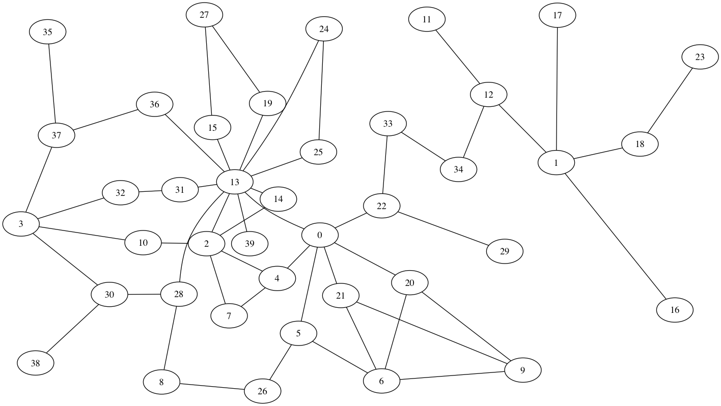
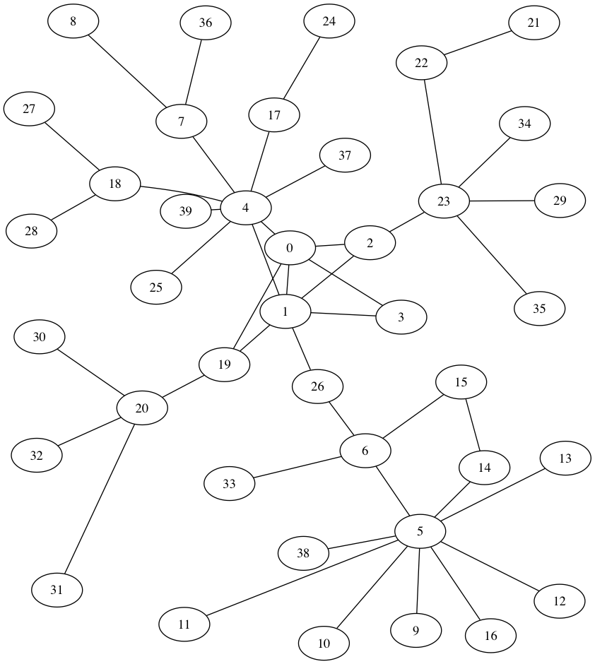
For each of the last 3 networks we extracted samples of 40 nodes using random-walk sampling according to Leskovec and Faloutsos [samplinglargegraphs] until 40 different nodes were visited and then we extracted the induced subgraph. Here we show two such samples for each dataset.

n	degree	closeness	betweenness	random-walk
1	{11}	{11}	{11}	{11}
2	{4, 11}	{2, 13} , {4, 11}	{4, 11}	{4, 11}
3	{4, 11, 13} , {0, 11, 13} , … (9)	{0, 11, 13} , {4, 11, 13} , … (4)	{4, 11, 13}	{0, 11, 13}
4	{2, 4, 11, 13} , … (23)	{2, 4, 11, 13} , … (5)]	{2, 4, 11, 13}	{2, 4, 11, 13}

Table 1: Solutions for group centrality on Proximity Semantic Network 1.

n	degree	closeness	betweenness	random-walk
1	{11}	{11}	{11}	{11}
2	{0, 11}	{2, 11} , … (2)	{2, 11}	{2, 11}
3	{2, 13, 21} , … (8)	{2, 13, 21}	{2, 11, 13}	{2, 13, 21}
4	{2, 4, 13, 21} , … (16)	{2, 4, 13, 21}	{2, 11, 13, 21}	{2, 4, 13, 21}

Table 2: Solutions for group centrality on Proximity Semantic Network 2.

n	degree	closeness	betweenness	random-walk
1	{6} , {17}	{6}	{17}	{6}
2	{0, 6}	{0, 6} , {10, 17}	{0, 6}	{0, 6}
3	{3, 13, 17} , {3, 10, 17}, … (10)	{3, 10, 17}	{0, 13, 17}	{3, 10, 17}
4	{0, 6, 10, 17} , … (18)	{0, 6, 10, 17} , … (6)	{0, 6, 10, 17}	{0, 6, 10, 17}

Table 3: Solutions for group centrality on Proximity Semantic Network constructed by non-biologist students.

n	degree	closeness	betweenness	random-walk
1	{12}	{12}	{12}	{12}
2	{3, 12}	{3, 12}	{3, 12}	{3, 12}
3	{3, 12, 19}, {3, 12, 21}	{3, 12, 21}, {3, 12, 22}	{3, 12, 19}, {3, 12, 21}	{3, 12, 22}
	{3, 12, 22}, {3, 12, 23}	{3, 12, 23}
4	{3, 12, 19, 23}	{3, 12, 19, 23}	{3, 12, 15, 19}, {3, 12, 15, 21}	{3, 5, 12, 22}

Table 4: Solutions for group centrality on Proximity Semantic Network constructed by biologist students.

n	degree	closeness	betweenness	random-walk
1	{4} , {20}	{4}	{20}	{4}
2	{4, 20}	{4, 20}	{4, 20}	{4, 20}
3	{4, 6, 20} , {6, 7, 20}	{0, 4, 20}	{4, 7, 20}	{4, 18, 20}
4	{4, 6, 18, 20} , {0, 4, 6, 20}	{0, 4, 6, 20}	{4, 6, 7, 20}	{4, 6, 18, 20}

Table 5: Solutions for group centrality on DBpedia sample 1.

n	degree	closeness	betweenness	random-walk
1	{13}	{13}	{13}	{13}
2	{0, 13} , {1, 13} , … (2)	{1, 13}	{0, 13}	{12, 13}
3	{0, 1, 13} , … (4)	{0, 1, 13}	{0, 1, 13}	{0, 1, 13}
4	{0, 1, 3, 13} , … (1)	{0, 1, 3, 13}	{0, 1, 3, 13}	{0, 1, 3, 13}

Table 6: Solutions for group centrality on DBpedia sample 2.

n	degree	closeness	betweenness	random-walk
1	{25}	{14}	{14}	{13}
2	{14, 25}	{5, 14} , {7, 13} , {7, 14} , {8, 13}	{14, 25}	{6, 14}
3	{4, 14, 25} , … (5)	{4, 14, 25} , … (4)	{4, 14, 25}	{0, 6, 14}
4	{0, 4, 14, 25} , … (10)	{1, 4, 14, 25} , … (2)	{4, 12, 14, 25}	{0, 4, 14, 25}

Table 7: Solutions for group centrality on Perception sample 1.

n	degree	closeness	betweenness	random-walk
1	{29} , … (1)	{15}	{1}	{29}
2	{2, 29}	{0, 15} , … (1)	{1, 2}	{29, 39}
3	{2, 8, 29} , … (3)	{0, 15, 32} , … (7)	{1, 2, 8}	{2, 8, 39}
4	{2, 8, 29, 39} , … (2)	{2, 26, 29, 39} , … (1)	{2, 8, 10, 29}	{2, 26, 29, 39}

Table 8: Solutions for group centrality on Perception sample 2.

n	degree	closeness	betweenness	random-walk
1	{10}	{35}	{35}	{10}
2	{10, 25}	{10, 25}	{25, 35}	{10, 25}
3	{10, 25, 39}	{10, 25, 39}	{10, 25, 35}	{10, 25, 39}
4	{10, 17, 25, 39} , … (87)	{10, 17, 25, 39} , … (87)	{10, 17, 25, 35}	{10, 17, 25, 39}

Table 9: Solutions for group centrality on Roget’s Thesaurus sample 1.

n	degree	closeness	betweenness	random-walk
1	{11}	{37}	{37}	{37}
2	{11, 14}	{14, 26}	{26, 37}	{14, 26}
3	{1, 14, 29} , … (6)	{11, 14, 29} , … (6)	{11, 26, 37}	{11, 14, 29}
4	{11, 14, 29, 37} , … (440)	{11, 14, 29, 37} , … (440)	{11, 14, 26, 37}	{11, 14, 29, 37}

Table 10: Solutions for group centrality on Roget’s Thesaurus sample 2.

3.2 Discussion of results

For each semantic network, and each centrality measure, we computed the optimal solutions of size 1, 2, 3, and 4. The results are presented in Tables 1 to 10. It is important to note that in some cases there were multiple candidates for optimal solution, but we only include at most two of them (if there are more than two solutions, there is a mark “… $(n)$” where $n$ is the number of extra solutions) .

From the results obtained, we can advance two main observations:

Robustness of group centrality. It is noticeable that in the samples the optimal solutions for all centrality measures become similar as the size $k$ of the set increases. Indeed, for groups of size 1, it can observed that there are networks for which the solution is different, depending on the centrality notion applied (e.g. Table 13). On the other hand, for groups of size 4, it can be observed that in most networks there is a common set of nodes selected by all four different measures used.

Non-ambiguity of group random-walk. As stated previously, for a given size $k$, more than one optimal solution may exist for group centrality. Moreover, from the results it can be inferred that as $k$ increases, so does the number of optimal candidates for certain particular measures. For example, Table 11 shows that degree and closeness centrality have 24 (resp. 6) optimal solutions of size 4. There is even an extreme case in Table 23, where degree and closeness have more than 400 different optimal group solutions. In a small sample of 40 nodes this variance does not help achieve the proposed goal. However, betweenness centrality seems to behave in general better in this matter (there is some dispersion, e.g. Table 14, but it is small). Random-walk centrality, on the other hand, is consistently better in this regard. In our sample selections, it is the only notion for which there is systematically a unique optimal solution for any size, and for all the networks.

4 Theoretical aspects of Group Centrality

As we saw in previous sections, group centrality offers interesting new insights on semantic networks. In this section we study the notion from a theoretical point of view, focusing in the complexity of computing it.

4.1 Complexity of Group Centrality

Let us define formally the problem of computing the most central set of nodes in a network under different centrality measures.

Definition 2 (Optimumset)

Given a graph $G=(V,E)$, a positive integer $k$ and a function $C:\mathcal{P}(V)\rightarrow\mathbb{R}$, define $optimumset(G,k,C)$ as the problem of finding a set $S\subset V$, of size $k$ such that

$$S\in\displaystyle\operatorname*{arg\,min}_{U\subset V;|U|=k}C(S).$$

For a real number $\alpha>0$, $optimumset(G,k,C,\alpha)$ will denote the corresponding decision problem: find if there exists a set $S\subset V$, of size $k$ such that $C(S)=\alpha$.

Theorem 2.  $optimumset(G,k,C,\alpha)$ is NP-complete for all four group centrality measures studied in this paper (that is, for $C\in\{C_{d},C_{c},C_{bc},h^{\swarrow}\}$).

Proof

First note that it is not difficult to prove that $C_{d}$, $C_{c}$ and $C_{bc}$ are all computable in polynomial time. Same for $h^{\swarrow}$ but we will leave that demonstration for later (see proposition 1). Thus the corresponding problems are all in NP.

Now, consider $\alpha=1$ and let $S_{d}$, $S_{c}$, $S_{bc}$ and $S_{h^{\swarrow}}$ be solutions of the corresponding decision problems.

Note that $C_{c}(S_{c})=1$ (resp. $C_{d}(S_{d})=1$) if and only if $S_{c}$ (resp. $S_{d}$) is a dominating set of cardinality $k$ in $G$. That is, the problem of finding a dominating set of cardinality $k$ in $G$ is polynomial time reducible to $optimumset(G,k,\alpha,C_{c})$ and $optimumset(G,k,\alpha,C_{d})$.

Indeed, $C_{c}(S_{c})=1$ if and only if $d(v,S_{c})=1,\forall v\notin S_{c}$, which happens if and only if every vertex $v\notin S_{c}$ has at least one neighbor on $S_{c}$ (which is also a necessary and sufficient condition for $C_{d}(S_{d})=1$). That is, $S_{c}$ (and also $S_{d}$) is a dominating set.

On the other hand, $C_{bc}(S_{bc})=1$ (resp. $C_{h^{\swarrow}}(S_{h^{\swarrow}})=1$) if and only if $S_{bc}$ (resp. $S_{h^{\swarrow}}$) is a vertex cover of $G$ of size $k$. That is, the problem of finding a vertex cover of $G$ of size $k$ is polynomial time reducible to $optimumset(G,k,\alpha,C_{h^{\swarrow}})$ and $optimumset(G,k,\alpha,C_{bc})$.

Indeed, $C_{bc}(S_{bc})=1$ if and only if $\sigma_{uv}(S_{bc})=\sigma_{uv},\forall u,v\notin S_{bc}$ with $u<v$, which occurs if and only if for every pair $\forall u,v\notin S_{bc}$ with $u<v$, all shortest paths that connect $u$ and $v$ have some vertex in $S_{bc}$. This is equivalent to having $N(v)\subseteq S_{bc}$ for all $v\in S_{bc}$. That is, $S_{bc}$ is a vertex cover of $G$.

Finally, $C_{h^{\swarrow}}(S_{h^{\swarrow}})=1$ if and only if $h(v,S_{h^{\swarrow}})=1,\forall v\notin S_{h^{\swarrow}}$, but $h(v,S_{h^{\swarrow}})=1$ occurs if and only if $N(v)\subset S,\forall v\notin S_{h^{\swarrow}}$. That is, $S_{h^{\swarrow}}$ is a vertex cover of $G$.

∎

4.2 Properties of Random Walk Centrality

Given a graph $G=(V,E)$, we can generalize the notion of random walk to the case where there is a weight function $\omega:E\rightarrow\mathbb{R}$ on the edges of $G$, by changing the transition probabilities for $p_{uv}=\omega(uv)/\omega(u)$, with $\omega(u)=\sum_{w\in N(u)}\omega(uw)$ (thus the case $\omega\equiv 1$ gives the original definition of random walk).

Note that the sequence of random vertices $(v_{t}:t=0,1,...)$ is a Markov chain. Let $P_{t}$ will denote the distribution of $v_{t}$: $P_{t}(v)=\mathbb{P}(v_{t}=v)$. The vertex $v_{0}$ may be fixed, but may also be drawn from an initial distribution $P_{0}$. This initial distribution is said to be $stationary$ if $P_{1}=P_{0}$ (which will imply that $P_{t}=P_{0}\ \forall t\geq 0$, because of the construction of the random walk). It can be easily proved that the distribution $\pi(v):=\omega(v)/\sum_{v\in V}\omega(w)$ is stationary for every graph $G$ and weight function $\omega$. From now on $\pi$ will be referred simply as the stationary distribution (it is not difficult to prove that this distribution is unique, which makes this reference valid).

Proposition 1

Given $G=(V,E)$, a weight function $\omega:E\rightarrow\mathbb{R}$, a subset $S\subset V$ and $v\in V$, then $h(v,S)$ and $h^{\swarrow}(S)$ can be computed in polynomial time.

For the proof, first we need the following result

Lemma 1

For a graph $G=(V,E)$, a weight function $\omega$ and $S\subseteq V$ define $G_{\scriptscriptstyle S}$ as the following weighted graph:

$V(G_{\scriptscriptstyle S})=(V\setminus S)\cup\{v_{\scriptscriptstyle S}\}$

$E(G_{\scriptscriptstyle S})=\{e\in E/e\cap S=\phi\}\cup\{e=uv_{\scriptscriptstyle S}/u\in V,N_{\scriptscriptstyle G}(u)\cap S\neq\phi\}$

and $\omega_{\scriptscriptstyle S}:\ E(G_{\scriptscriptstyle S})\longrightarrow\mathbb{N}$ defined as: $\omega_{\scriptscriptstyle S}(uv)=\omega(uv)$ if $uv\cap S=\emptyset$. Otherwise, i.e. if $v=v_{\scriptscriptstyle S}$, then $\omega_{\scriptscriptstyle S}(uv)=\sum\limits_{w\in N_{\scriptscriptstyle G}(u)\cap S}\omega(uw)$.

Then for $u\in V\setminus S$ we have that $H_{\scriptscriptstyle G}(u,S)=H_{{\scriptscriptstyle G}_{\scriptscriptstyle S}}(u,v_{\scriptscriptstyle S}).$

Proof

For a vertex $w\in V\setminus S$, let $T_{w,S}$ and $T_{w,v_{S}}$ be two random variables that count the number of steps that a random walk (on $G$ and $G_{S}$ respectively) starting at vertex $w$ takes in order to reach some vertex of $S$ and $v_{\scriptscriptstyle S}$ (respectively) for the first time. We will prove that $T_{u,S}$ and $T_{u,v_{S}}$ have the same distribution.

Let us proceed by induction on the possible values of $T_{u,S}$ and $T_{u,v_{\scriptscriptstyle S}}$.

If $n=1$ then

$$\mathbb{P}(T_{u,S}=1)=\frac{\sum\limits_{w\in N_{G}(u)\cap S}\omega(uw)}{\omega(u)}=\frac{\omega_{\scriptscriptstyle S}(uv_{\scriptscriptstyle S})}{\omega_{\scriptscriptstyle S}(u)}=\mathbb{P}(T_{u,v_{\scriptscriptstyle S}}=1).$$

Let $n>1$ and assume that the property holds for $n-1$. Then

$$\mathbb{P}(T_{u,S}=n) =\sum_{w\in V\setminus S}\frac{\omega(uw)}{\omega(u)}\mathbb{P}(T_{w,S}=n-1)$$

$$=\sum_{w\in V\setminus S}\frac{\omega(uw)}{\omega(u)}\mathbb{P}(T_{w,v_{S}}=n-1)$$

$$=\sum_{w\in V(G_{S})\setminus v_{S}}\frac{\omega(uw)}{\omega(u)}(T_{w,v_{S}}=n-1)$$

$$=\sum_{w\in V(G_{S})\setminus v_{S}}\frac{\omega_{\scriptscriptstyle S}(uw)}{\omega_{\scriptscriptstyle S}(u)}\mathbb{P}(T_{w,v_{S}}=n-1)=\mathbb{P}(T_{u,v_{S}}=n).$$

Using this we have that $H_{\scriptscriptstyle G}(u,S)=\mathbb{E}(T_{u,S})=\mathbb{E}(T_{u,v_{S}})=H_{{\scriptscriptstyle G}_{S}}(u,v_{S}).$ ∎

Proof (of proposition 1)

Let $P$ be the probability transition matrix associated to a random walk on $G$, and the function $\omega$. That is, $P_{ij}=\frac{\omega(ij)}{\omega(i)}$. Define $P_{\infty}$ as

$$P_{\infty} =\begin{pmatrix}\pi(1)&\pi(2)&\dots&\pi(n)\\ \vdots&\vdots&\dots&\vdots\\ \pi(1)&\pi(2)&\dots&\pi(n)\end{pmatrix}.$$

where $\pi$ is the stationary distribution. Define also $Z:=(I-(P-P_{\infty}))^{-1}$ and let $H$ be the hitting time matrix of $G$, that is, $H_{ij}=H_{\scriptscriptstyle G}(i,j)$. Then it can be proved as stated in [17] that for $i,j\in V$

$$H_{\scriptscriptstyle G}(i,j)=\frac{Z_{\scriptstyle{jj}}-Z_{\scriptstyle{ij}}}{\pi(j)}.$$ (1)

Therefore, by combining equation (1) and lemma 1 we can compute $h(v,S)$ by inverting a suitable matrix $Z$, which can be made in polynomial time. ∎

Lemma 2

There is a parameterized family of graphs for which Random walk centrality behaves systematically differently than degree, closeness and betweenness group centrality.

Proof

Consider $\{G_{n}^{m}\}$, with $n,m\in\mathbb{Z}^{+}$ and $n<<m$ a family of graphs constructed as follows (see Fig. 2): for $i\in\{1,...,m-1\}$, $K_{n}^{i}$ is a subgraph of $G_{n}^{m}$ that is a $n$-clique and that is connected to $v$ through an unique vertex $k_{n}^{i}$. On the other hand, $T_{n}^{i}$ is a subtree of $G_{n}^{m}$ of height 1 and size $n$ with root $t_{i}^{n}$ the only vertex in $T_{n}^{i}$ that is neighbor of $v$ in $G_{n}^{m}$. Suppose we want to find a set $S$ that solves $optimumset(G_{n}^{m},m+1,C)$ for $C\in\{C_{d},C_{c},C_{bc},h^{\swarrow}\}$. It is not difficult to prove that for group closeness and betweenness centrality the sets $S_{K}=\{v,k_{n}^{1},...,k_{n}^{m}\}$ and $S_{T}=\{v,t_{n}^{1},...,t_{n}^{m}\}$ are solutions. For group degree centrality $\bar{S}_{K}=\{t_{n}^{j},k_{n}^{1},...,k_{n}^{m}\}$ and $\bar{S}_{T}=\{k_{n}^{j},t_{n}^{1},...,t_{n}^{m}\}$ for any $1\leq j\leq m$ are possible solutions. However, one could argue the difference in connectivity between sets $S_{K}$ and $S_{T}$ should be accounted for. Indeed, for random walk centrality, $S_{k}$ (a more connected version of $S_{t}$) is the only solution. ∎

Figure 2: Which set of size $m+1$ is more central? $S_{K}$ or $S_{T}$?

The following bound shows an interesting relation between random walk centrality, degree and closeness

Proposition 2

There exists a real constant $c>0$ such that for $S\subset V$

$$h^{\swarrow}(S)\;\leq\;\frac{1}{|V\setminus S|}\left(\sum_{u\in V\setminus S}d(u,S)\right)\left(\sum_{v\in V\setminus S}d(v)\right)\leq c|V\setminus S|^{3}.$$

Proof

Define $\partial(S):=\{v\in S:\exists u\in V\setminus S,uv\in E\}$. Define the subgraph $G_{S}$ of $G$ as follows: $V(G_{S}):=(V\setminus S)\cup\partial(S)$ and $E(G_{S}):=\{uv\in E:u,v\in V(G_{S})\wedge u\in V\setminus S\}$.

First note that for any pair of vertices $u\in V\setminus S$ and $v\in\partial(S)$

$$H_{G}(u,S)=H_{G_{S}}(u,\partial(S))\leq H_{G_{S}}(u,v).$$

The equality follows from the fact that the subgraph traversed and the target hit in both expressions are the same, and the inequality holds because the target of the expression on the right is more difficult to hit, thus needs more walking around.

Using this, we have that

$$h^{\swarrow}(S)=\frac{\sum_{u\in V\setminus S}H_{G}(u,S)}{|V\setminus S|}\leq\frac{\sum_{u\in V\setminus S}H_{G_{S}}(u,v_{u})}{|V\setminus S|},$$

with each $v_{u}\in\partial(S)$ chosen such that $d_{G_{S}}(u,v_{u})=d_{G}(u,S)$.

On the other hand, by using the known fact that for any graph $L$ and any pair of vertices $u,v\in V(L)$, $H_{L}(u,v)\leq 2|E(L)|d_{L}(u,v)$, we have that

$$\frac{\sum_{u\in V\setminus S}H_{G_{S}}(u,v)}{|V\setminus S|} \leq\frac{\sum_{u\in V\setminus S}2|E(G_{S})|d_{G_{S}}(u,v_{u})}{|V\setminus S|}$$

$$\leq\frac{1}{|V\setminus S|}\left(\sum_{u\in V\setminus S}d_{G}(u,S)\right)\left(\sum_{v\in V\setminus S}d_{G}(v)\right).\;\squareforqed$$

5 Conclusions

We perform a SWOT analysis of the application of the notion of group centrality to semantic networks, putting a particular focus on random walk group centrality. The challenges faced were mainly of two types. First, the ambiguity of the very notion of the “most central” concept in a semantic network; and second, the size of the networks.

In spite of these obstacles (that we discussed in the paper), we hope we presented enough evidence that this topic deserves to be explored and researched. We approached these obstacles by working with small samples and advancing theoretical results. Besides stating the problem at the formal level, we proved that the problem of computing group centrality is NP-hard, and showed that random walk centrality comes up as a good candidate for capturing the notion of centrality on semantic networks.

The above opens at least two lines of research on this topic: First, to find good approximation algorithms to compute group centrality particularly for random walk centrality. Second, the task of building a good benchmark of big semantic networks together with their candidate sets to match the most important concepts in the network.

Appendix 0.A Appendix

Figure 3: Proximity Semantic Network 1.

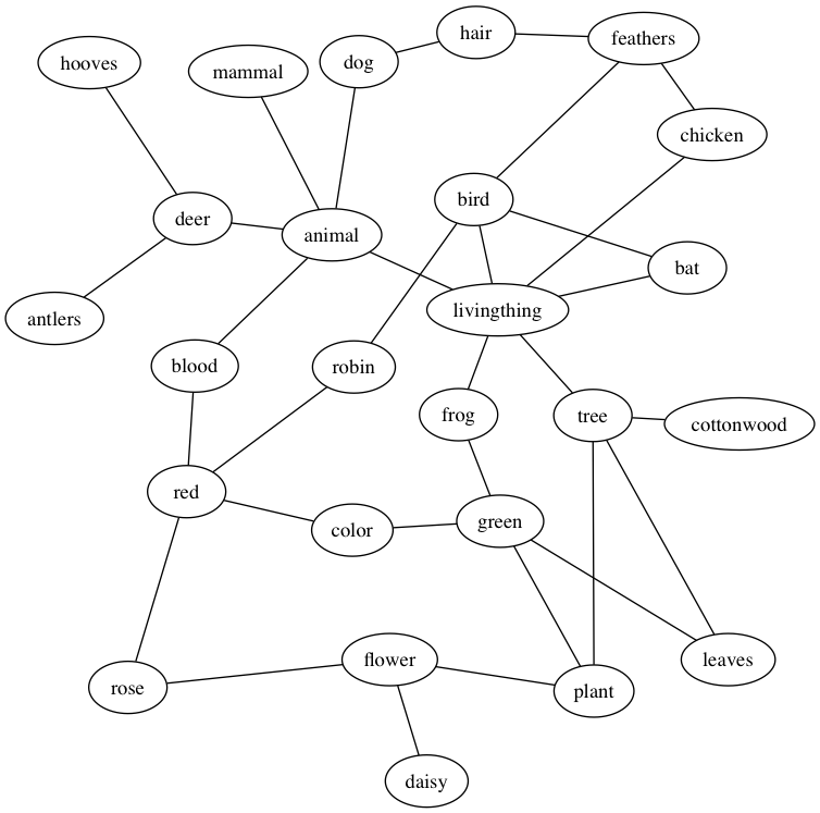
Proximity Semantic Network 1 Labels:

• 0.- animal

• 1.- antlers

• 2.- bat

• 3.- bird

• 4.- blood

• 5.- chicken

• 6.- color

• 7.- cottonwood

• 8.- daisy

• 9.- deer

• 10.- dog

• 11.- feathers

• 12.- flower

• 13.- frog

• 14.- green

• 15.- hair

• 16.- hooves

• 17.- leaves

• 18.- livingthing

• 19.- mammal

• 20.- plant

• 21.- red

• 22.- robin

• 23.- rose

• 24.- tree

n	degree	closeness	betweenness	random-walk
1	{11}	{11}	{11}	{11}
2	{4, 11}	{2, 13} , {4, 11}	{4, 11}	{4, 11}
3	{4, 11, 13} , {0, 11, 13} , … (9)	{0, 11, 13} , {4, 11, 13} , … (4)	{4, 11, 13}	{0, 11, 13}
4	{2, 4, 11, 13} , … (23)	{2, 4, 11, 13} , … (5)]	{2, 4, 11, 13}	{2, 4, 11, 13}

Table 11: Solutions for group centrality on Proximity Semantic Network 1.

Figure 4: Proximity Semantic Network 2.

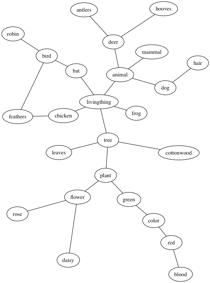
Proximity Semantic Network 2 Labels:

• 0.- animal

• 1.- antlers

• 2.- bat

• 3.- bird

• 4.- blood

• 5.- chicken

• 6.- color

• 7.- cottonwood

• 8.- daisy

• 9.- deer

• 10.- dog

• 11.- feathers

• 12.- flower

• 13.- frog

• 14.- green

• 15.- hair

• 16.- hooves

• 17.- leaves

• 18.- livingthing

• 19.- mammal

• 20.- plant

• 21.- red

• 22.- robin

• 23.- rose

• 24.- tree

n	degree	closeness	betweenness	random-walk
1	{11}	{11}	{11}	{11}
2	{0, 11}	{2, 11} , … (2)	{2, 11}	{2, 11}
3	{2, 13, 21} , … (8)	{2, 13, 21}	{2, 11, 13}	{2, 13, 21}
4	{2, 4, 13, 21} , … (16)	{2, 4, 13, 21}	{2, 11, 13, 21}	{2, 4, 13, 21}

Table 12: Solutions for group centrality on Proximity Semantic Network 2.

Figure 5: Proximity network built by non-specialists.

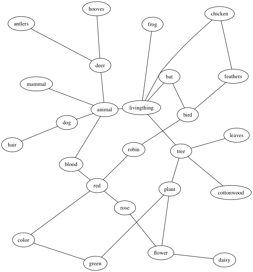
Proximity network built by non-specialists labels:

• 0.- animal

• 1.- antlers

• 2.- bat

• 3.- bird

• 4.- blood

• 5.- chicken

• 6.- color

• 7.- cottonwood

• 8.- daisy

• 9.- deer

• 10.- dog

• 11.- feathers

• 12.- flower

• 13.- frog

• 14.- green

• 15.- hair

• 16.- hooves

• 17.- leaves

• 18.- livingthing

• 19.- mammal

• 20.- plant

• 21.- red

• 22.- robin

• 23.- rose

• 24.- tree

n	degree	closeness	betweenness	random-walk
1	{6} , {17}	{6}	{17}	{6}
2	{0, 6}	{0, 6} , {10, 17}	{0, 6}	{0, 6}
3	{3, 13, 17} , {3, 10, 17}, … (10)	{3, 10, 17}	{0, 13, 17}	{3, 10, 17}
4	{0, 6, 10, 17} , … (18)	{0, 6, 10, 17} , … (6)	{0, 6, 10, 17}	{0, 6, 10, 17}

Table 13: Solutions for group centrality on Proximity Semantic Network constructed by non-biologist students.

Figure 6: Proximity network built by biologists.

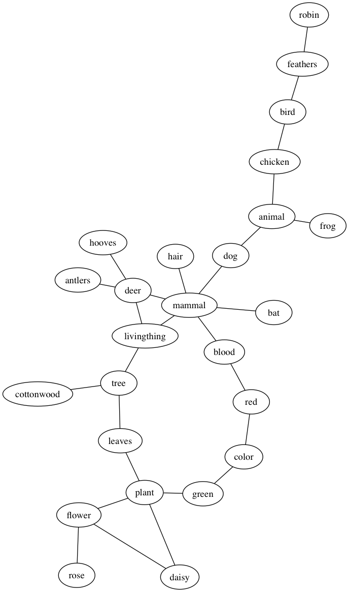
Proximity network built by biologists labels:

• 0.- animal

• 1.- antlers

• 2.- bat

• 3.- bird

• 4.- blood

• 5.- chicken

• 6.- color

• 7.- cottonwood

• 8.- daisy

• 9.- deer

• 10.- dog

• 11.- feathers

• 12.- flower

• 13.- frog

• 14.- green

• 15.- hair

• 16.- hooves

• 17.- leaves

• 18.- livingthing

• 19.- mammal

• 20.- plant

• 21.- red

• 22.- robin

• 23.- rose

• 24.- tree

n	degree	closeness	betweenness	random-walk
1	{12}	{12}	{12}	{12}
2	{3, 12}	{3, 12}	{3, 12}	{3, 12}
3	{3, 12, 19}, {3, 12, 21}	{3, 12, 21}, {3, 12, 22}	{3, 12, 19}, {3, 12, 21}	{3, 12, 22}
	{3, 12, 22}, {3, 12, 23}	{3, 12, 23}
4	{3, 12, 19, 23}	{3, 12, 19, 23}	{3, 12, 15, 19}, {3, 12, 15, 21}	{3, 5, 12, 22}

Table 14: Solutions for group centrality on Proximity Semantic Network constructed by biologist students.

Figure 7: Sample 1 from Perception Network.

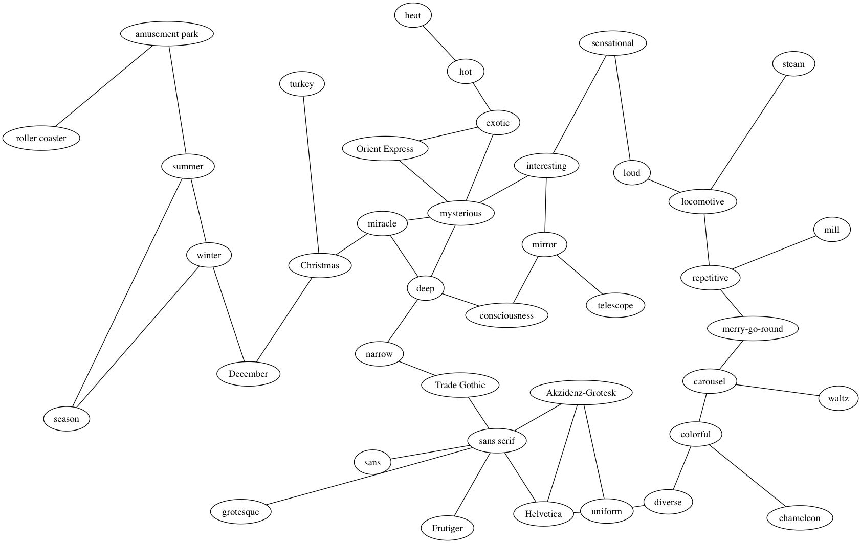
Sample 1 from Perception network labels:

• 0.- Akzidenz-Grotesk

• 1.- Christmas

• 2.- December

• 3.- Frutiger

• 4.- Helvetica

• 5.- Orient Express

• 6.- Trade Gothic

• 7.- amusement park

• 8.- carousel

• 9.- chameleon

• 10.- colorful

• 11.- consciousness

• 12.- deep

• 13.- diverse

• 14.- exotic

• 15.- grotesque

• 16.- heat

• 17.- hot

• 18.- interesting

• 19.- locomotive

• 20.- loud

• 21.- merry-go-round

• 22.- mill

• 23.- miracle

• 24.- mirror

• 25.- mysterious

• 26.- narrow

• 27.- repetitive

• 28.- roller coaster

• 29.- sans

• 30.- sans serif

• 31.- season

• 32.- sensational

• 33.- steam

• 34.- summer

• 35.- telescope

• 36.- turkey

• 37.- uniform

• 38.- waltz

• 39.- winter

n	degree	closeness	betweenness	random-walk
1	{25}	{14}	{14}	{13}
2	{14, 25}	{5, 14} , {7, 13} , {7, 14} , {8, 13}	{14, 25}	{6, 14}
3	{4, 14, 25} , … (5)	{4, 14, 25} , … (4)	{4, 14, 25}	{0, 6, 14}
4	{0, 4, 14, 25} , … (10)	{1, 4, 14, 25} , … (2)	{4, 12, 14, 25}	{0, 4, 14, 25}

Table 15: Solutions for group centrality on Perception sample 1.

Figure 8: Sample 2 from Perception Network.

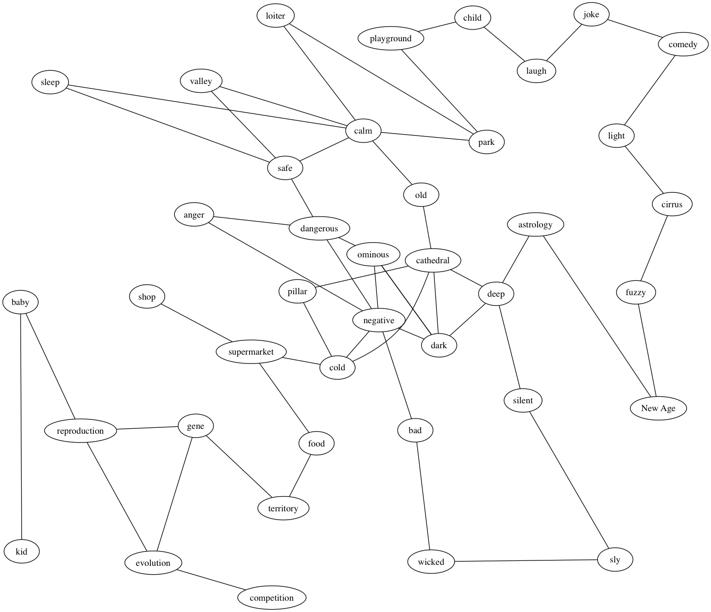
Sample 2 from Perception network labels:

• 0.- New Age

• 1.- anger

• 2.- astrology

• 3.- baby

• 4.- bad

• 5.- calm

• 6.- cathedral

• 7.- child

• 8.- cirrus

• 9.- cold

• 10.- comedy

• 11.- competition

• 12.- dangerous

• 13.- dark

• 14.- deep

• 15.- evolution

• 16.- food

• 17.- fuzzy

• 18.- gene

• 19.- joke

• 20.- kid

• 21.- laugh

• 22.- light

• 23.- loiter

• 24.- negative

• 25.- old

• 26.- ominous

• 27.- park

• 28.- pillar

• 29.- playground

• 30.- reproduction

• 31.- safe

• 32.- shop

• 33.- silent

• 34.- sleep

• 35.- sly

• 36.- supermarket

• 37.- territory

• 38.- valley

• 39.- wicked

n	degree	closeness	betweenness	random-walk
1	{29} , … (1)	{15}	{1}	{29}
2	{2, 29}	{0, 15} , … (1)	{1, 2}	{29, 39}
3	{2, 8, 29} , … (3)	{0, 15, 32} , … (7)	{1, 2, 8}	{2, 8, 39}
4	{2, 8, 29, 39} , … (2)	{2, 26, 29, 39} , … (1)	{2, 8, 10, 29}	{2, 26, 29, 39}

Table 16: Solutions for group centrality on Perception sample 2.

Figure 9: Sample 3 from Perception Network.

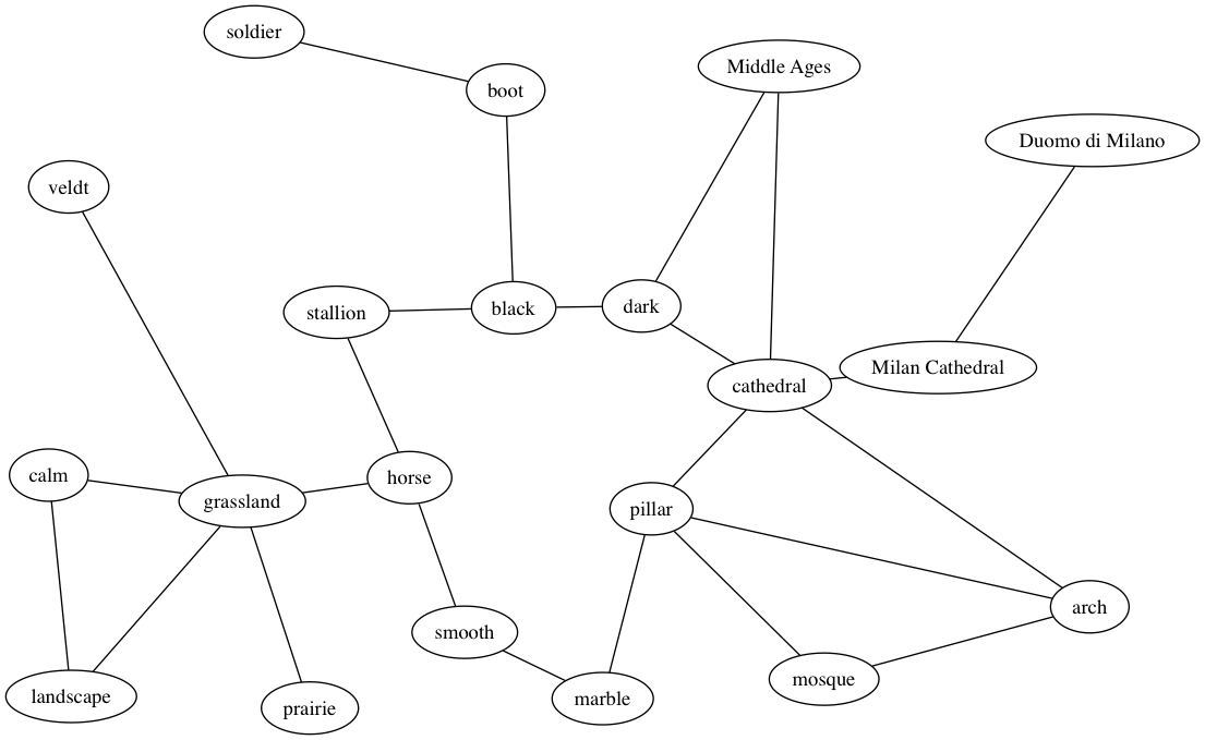
Sample 3 from Perception network labels:

• 0.- Duomo di Milano

• 1.- Middle Ages

• 2.- Milan Cathedral

• 3.- arch

• 4.- black

• 5.- boot

• 6.- calm

• 7.- cathedral

• 8.- dark

• 9.- grassland

• 10.- horse

• 11.- landscape

• 12.- marble

• 13.- mosque

• 14.- pillar

• 15.- prairie

• 16.- smooth

• 17.- soldier

• 18.- stallion

• 19.- veldt

n	degree	closeness	betweenness	random-walk
1	{11}	{11}	{11}	{11}
2	{4, 11}	{2, 13} , {4, 11}	{4, 11}	{4, 11}
3	{0, 11, 13} , {4, 11, 13} , … (9)	{0, 11, 13} , {4, 11, 13} , … (4)	{4, 11, 13}	{0, 11, 13}
4	{2, 4, 11, 13} , … (23)	{2, 4, 11, 13} , … (5)	{2, 4, 11, 13}	{2, 4, 11, 13}

Table 17: Solutions for group centrality on Perception sample 3.

Figure 10: Sample 1 from DBpedia Categories network.

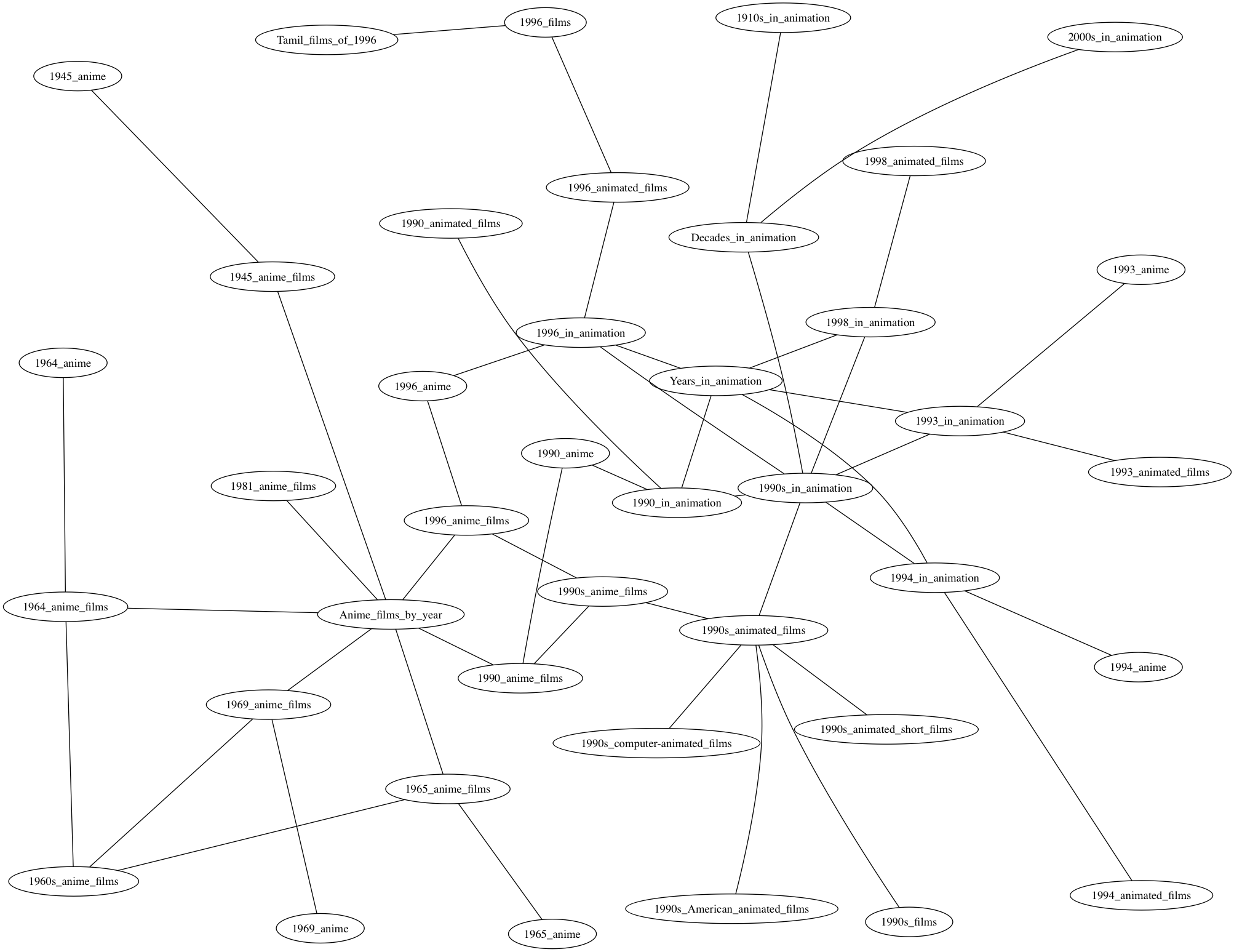
Sample 1 from DBpedia Categories network labels:

• 0.- 1996_films

• 1.- 1990s_films

• 2.- 2000s_in_animation

• 3.- Decades_in_animation

• 4.- 1990s_in_animation

• 5.- 1910s_in_animation

• 6.- 1990s_animated_films

• 7.- Years_in_animation

• 8.- 1964_anime

• 9.- 1965_anime

• 10.- 1969_anime

• 11.- 1990_anime

• 12.- 1990_in_animation

• 13.- 1993_anime

• 14.- 1993_in_animation

• 15.- 1994_anime

• 16.- 1994_in_animation

• 17.- 1996_anime

• 18.- 1996_in_animation

• 19.- 1998_in_animation

• 20.- Anime_films_by_year

• 21.- 1990_anime_films

• 22.- 1990s_anime_films

• 23.- 1996_anime_films

• 24.- 1981_anime_films

• 25.- 1960s_anime_films

• 26.- 1998_animated_films

• 27.- 1996_animated_films

• 28.- 1994_animated_films

• 29.- 1993_animated_films

• 30.- 1990_animated_films

• 31.- 1965_anime_films

• 32.- 1969_anime_films

• 33.- 1945_anime_films

• 34.- 1945_anime

• 35.- 1990s_American_animated_films

• 36.- 1990s_animated_short_films

• 37.- Tamil_films_of_1996

• 38.- 1964_anime_films

• 39.- 1990s_computer-animated_films

n	degree	closeness	betweenness	random-walk
1	{4} , {20}	{4}	{20}	{4}
2	{4, 20}	{4, 20}	{4, 20}	{4, 20}
3	{4, 6, 20} , {6, 7, 20}	{0, 4, 20}	{4, 7, 20}	{4, 18, 20}
4	{4, 6, 18, 20} , {0, 4, 6, 20}	{0, 4, 6, 20}	{4, 6, 7, 20}	{4, 6, 18, 20}

Table 18: Solutions for group centrality on DBpedia sample 1.

Figure 11: Sample 2 from DBpedia Categories network.

Sample 2 from DBpedia Categories network labels:

• 0.- Wikipedia_categories_named_after_populated_places_in_Italy

• 1.- Provinces_of_Italy

• 2.- Cities_and_towns_in_Emilia-Romagna

• 3.- Emilia-Romagna

• 4.- Parma

• 5.- Turin

• 6.- Cities_and_towns_in_Piedmont

• 7.- Communes_of_the_Province_of_Parma

• 8.- Education_in_Italy_by_city

• 9.- Communes_of_the_Province_of_Alessandria

• 10.- Geography_of_Emilia-Romagna

• 11.- Province_of_Pavia_geography_stubs

• 12.- Province_of_Pavia

• 13.- Bologna

• 14.- Communes_of_the_Province_of_Bologna

• 15.- Buildings_and_structures_in_Bologna

• 16.- Province_of_Arezzo

• 17.- Province_of_Ancona

• 18.- Province_of_Lucca

• 19.- Visitor_attractions_in_Bologna

• 20.- Tortona

• 21.- Novi_Ligure

• 22.- Pavia

• 23.- Communes_of_the_Province_of_Lucca

• 24.- Roman_Catholic_archbishops_of_Bologna

• 25.- History_of_Bologna

• 26.- Education_in_Turin

• 27.- Palaces_in_Bologna

• 28.- Education_in_Bologna

• 29.- University_of_Pavia

• 30.- Education_in_Emilia-Romagna

• 31.- Culture_in_Bologna

• 32.- Culture_in_Emilia-Romagna

• 33.- Buildings_and_structures_in_Pavia

• 34.- Buildings_and_structures_in_the_Province_of_Pavia

• 35.- Companies_by_region_of_Italy

• 36.- Companies_based_in_Bologna

• 37.- Companies_based_in_Emilia-Romagna

• 38.- Education_in_Italy_by_region

• 39.- Media_in_Bologna

n	degree	closeness	betweenness	random-walk
1	{13}	{13}	{13}	{13}
2	{0, 13} , {1, 13} , … (2)	{1, 13}	{0, 13}	{12, 13}
3	{0, 1, 13} , … (4)	{0, 1, 13}	{0, 1, 13}	{0, 1, 13}
4	{0, 1, 3, 13} , … (1)	{0, 1, 3, 13}	{0, 1, 3, 13}	{0, 1, 3, 13}

Table 19: Solutions for group centrality on DBpedia sample 2.

Figure 12: Sample 3 from DBpedia Categories network.

Sample 3 from DBpedia Categories network labels:

• 0.- Neognathae

• 1.- Birds_by_classification

• 2.- Procellariiformes

• 3.- Phoenicopteriformes

• 4.- Pelecaniformes

• 5.- Hornbills

• 6.- Bucerotidae

• 7.- Ardeidae

• 8.- Egretta

• 9.- Aceros

• 10.- Anthracoceros

• 11.- Buceros

• 12.- Ceratogymna

• 13.- Ocyceros

• 14.- Penelopides

• 15.- Bucerotinae

• 16.- Tockus

• 17.- Phalacrocoracidae

• 18.- Fregatidae

• 19.- Falconiformes

• 20.- Accipitridae

• 21.- Oceanodroma

• 22.- Hydrobatinae

• 23.- Hydrobatidae

• 24.- Phalacrocorax

• 25.- Plotopteridae

• 26.- Bucerotiformes

• 27.- Limnofregata

• 28.- Fregata

• 29.- Oceanitinae

• 30.- Aviceda

• 31.- Dryotriorchis

• 32.- Erythrotriorchis

• 33.- Anorrhinus

• 34.- Fregetta

• 35.- Oceanites

• 36.- Botaurus

• 37.- Anhingidae

• 38.- Rhyticeros

• 39.- Pelecanus

n	degree	closeness	betweenness	random-walk
1	{5}	{1}	{1}	{1}
2	{4, 5}	{1, 5}	{4, 5}	{1, 5}
3	{4, 5, 23}	{4, 5, 23}	{4, 5, 23}	{4, 5, 23}
4	{4, 5, 20, 23}	{4, 5, 20, 23}	{4, 5, 20, 23}	{4, 5, 20, 23}

Table 20: Solutions for group centrality on DBpedia sample 3.

Figure 13: Sample 1 from Roget’s Thesaurus network.

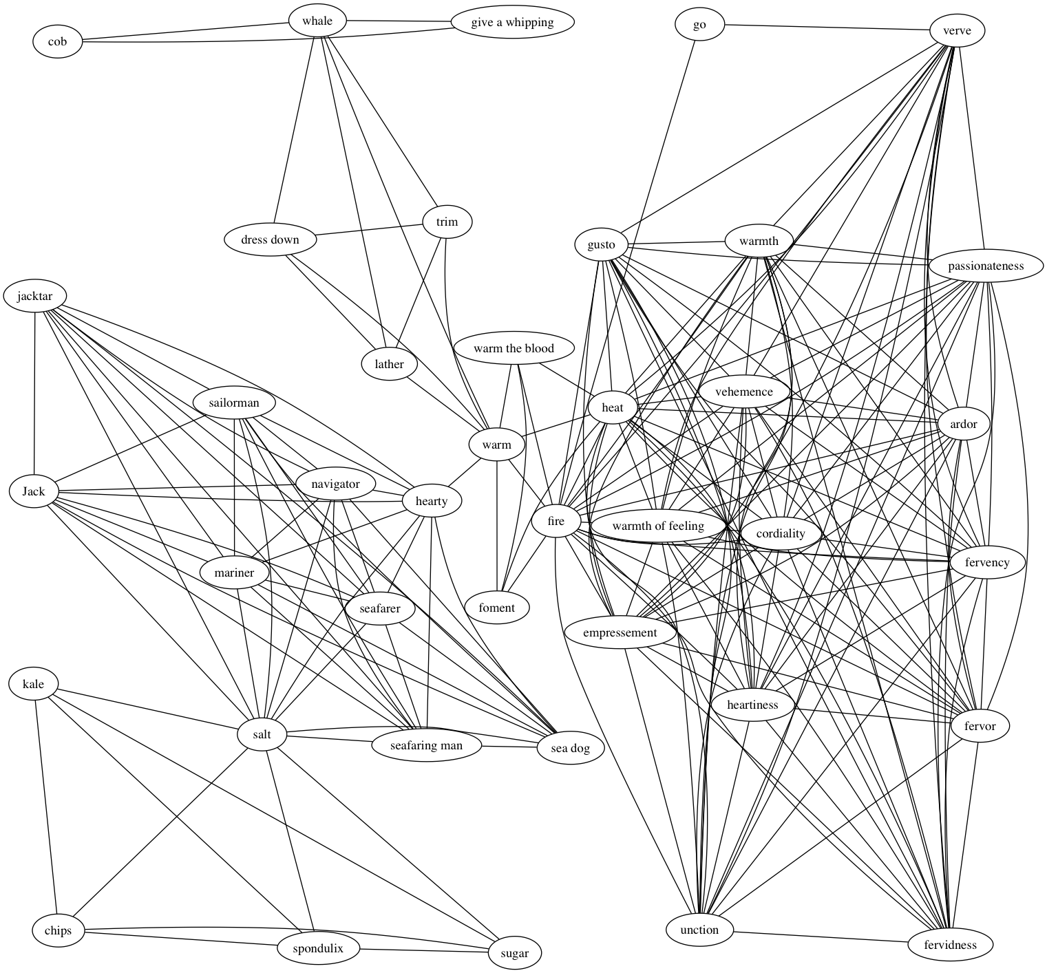
Sample 1 from Roget’s Thesaurus network labels:

• 0.- Jack

• 1.- ardor

• 2.- chips

• 3.- cob

• 4.- cordiality

• 5.- dress down

• 6.- empressement

• 7.- fervency

• 8.- fervidness

• 9.- fervor

• 10.- fire

• 11.- foment

• 12.- give a whipping

• 13.- go

• 14.- gusto

• 15.- heartiness

• 16.- hearty

• 17.- heat

• 18.- jacktar

• 19.- kale

• 20.- lather

• 21.- mariner

• 22.- navigator

• 23.- passionateness

• 24.- sailorman

• 25.- salt

• 26.- sea dog

• 27.- seafarer

• 28.- seafaring man

• 29.- spondulix

• 30.- sugar

• 31.- trim

• 32.- unction

• 33.- vehemence

• 34.- verve

• 35.- warm

• 36.- warm the blood

• 37.- warmth

• 38.- warmth of feeling

• 39.- whale

n	degree	closeness	betweenness	random-walk
1	{10}	{35}	{35}	{10}
2	{10, 25}	{10, 25}	{25, 35}	{10, 25}
3	{10, 25, 39}	{10, 25, 39}	{10, 25, 35}	{10, 25, 39}
4	{10, 17, 25, 39} , … (87)	{10, 17, 25, 39} , … (87)	{10, 17, 25, 35}	{10, 17, 25, 39}

Table 21: Solutions for group centrality on Roget’s Thesaurus sample 1.

Figure 14: Sample 2 from Roget’s Thesaurus network.

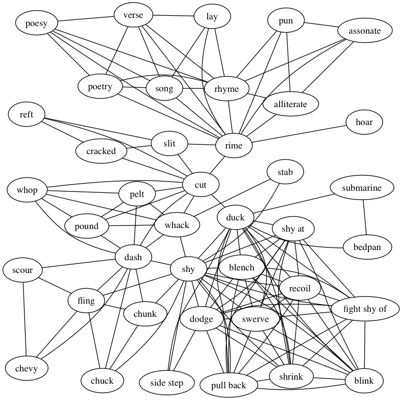
Sample 2 from Roget’s Thesaurus network labels:

• 0.- alliterate

• 1.- assonate

• 2.- bedpan

• 3.- blench

• 4.- blink

• 5.- chevy

• 6.- chuck

• 7.- chunk

• 8.- cracked

• 9.- cut

• 10.- dash

• 11.- dodge

• 12.- duck

• 13.- fight shy of

• 14.- fling

• 15.- hoar

• 16.- lay

• 17.- pelt

• 18.- poesy

• 19.- poetry

• 20.- pound

• 21.- pull back

• 22.- pun

• 23.- recoil

• 24.- reft

• 25.- rhyme

• 26.- rime

• 27.- scour

• 28.- shrink

• 29.- shy

• 30.- shy at

• 31.- side step

• 32.- slit

• 33.- song

• 34.- stab

• 35.- submarine

• 36.- swerve

• 37.- verse

• 38.- whack

• 39.- whop

n	degree	closeness	betweenness	random-walk
1	{29}	{9}	{9}	{29}
2	{26, 29}	{26, 29}	{9, 29}	{26, 29}
3	{10, 12, 26}	{10, 12, 26}	{9, 26, 29}	{10, 12, 26}
4	{10, 12, 26, 32} , … (4)	{10, 12, 24, 26} , … (4)	{10, 12, 26, 29}	{10, 12, 26, 29}

Table 22: Solutions for group centrality on Roget’s Thesaurus sample 2.

Figure 15: Sample 3 from Roget’s Thesaurus network.

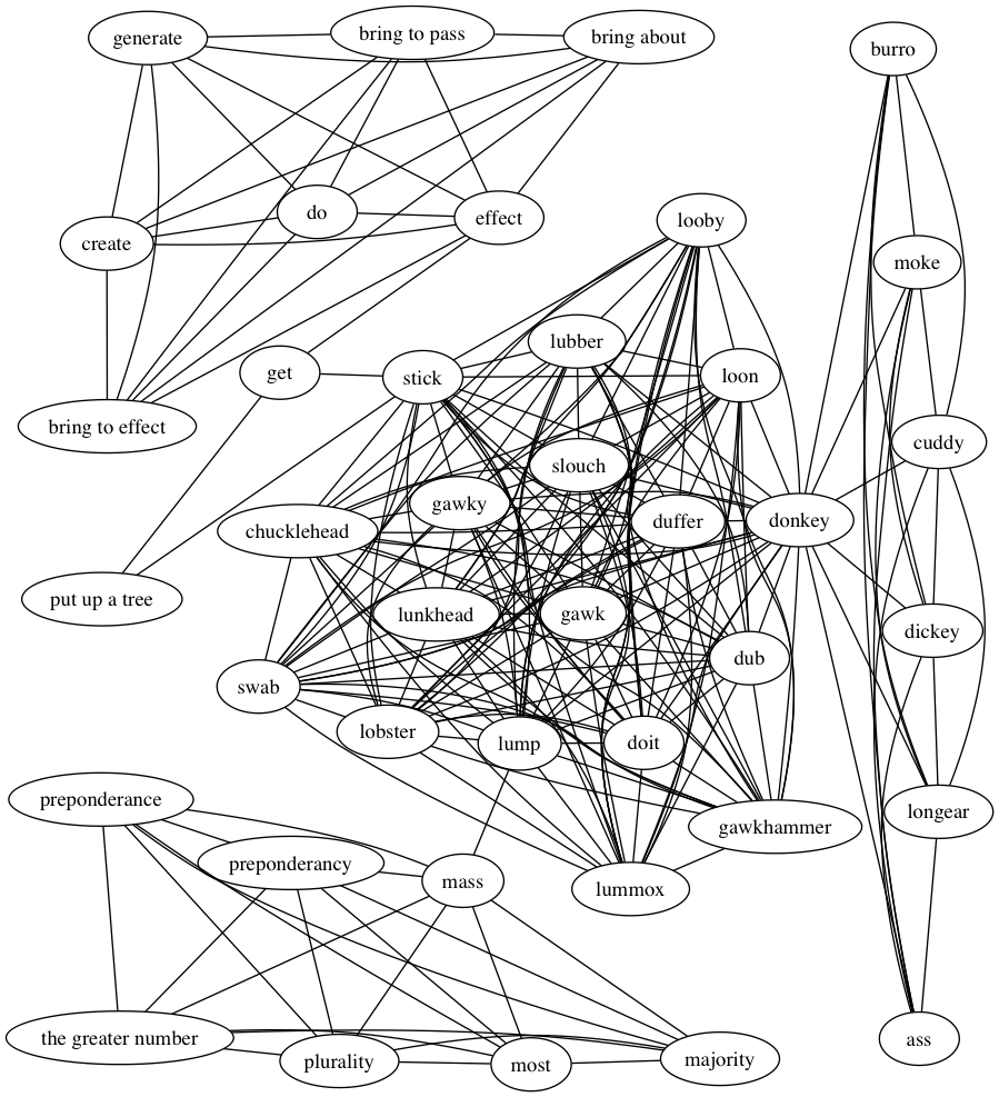
Sample 3 from Roget’s Thesaurus network labels:

• 0.- ass

• 1.- bring about

• 2.- bring to effect

• 3.- bring to pass

• 4.- burro

• 5.- chucklehead

• 6.- create

• 7.- cuddy

• 8.- dickey

• 9.- do

• 10.- doit

• 11.- donkey

• 12.- dub

• 13.- duffer

• 14.- effect

• 15.- gawk

• 16.- gawkhammer

• 17.- gawky

• 18.- generate

• 19.- get

• 20.- lobster

• 21.- longear

• 22.- looby

• 23.- loon

• 24.- lubber

• 25.- lummox

• 26.- lump

• 27.- lunkhead

• 28.- majority

• 29.- mass

• 30.- moke

• 31.- most

• 32.- plurality

• 33.- preponderance

• 34.- preponderancy

• 35.- put up a tree

• 36.- slouch

• 37.- stick

• 38.- swab

• 39.- the greater number

n	degree	closeness	betweenness	random-walk
1	{11}	{37}	{37}	{37}
2	{11, 14}	{14, 26}	{26, 37}	{14, 26}
3	{1, 14, 29} , … (6)	{11, 14, 29} , … (6)	{11, 26, 37}	{11, 14, 29}
4	{11, 14, 29, 37} , … (440)	{11, 14, 29, 37} , … (440)	{11, 14, 26, 37}	{11, 14, 29, 37}

Table 23: Solutions for group centrality on Roget’s Thesaurus sample 3.

References

- [1] DBpedia. http://www.dbpedia.org.
- [2] J. Abbott, J. Austerweil, T. Griffiths. Human memory search as a random walk in a semantic network. Adv. Neur. Inf. Proc. Syst. 25, 3050-58, 2012.
- [3] G. Cheng, Th. Tran, Y. Qu. RELIN: Relatedness and Informativeness-based Centrality for Entity Summarization. ISWC 2011, Springer 2011.
- [4] L. Ding, R. Pan, T. Finin, A. Joshi, Y. Peng, P. Kolari. Finding and ranking knowledge on the semantic web. In ISWC 2005, 156–170. Springer, 2005.
- [5] M. G. Everett, S. P. Borgatti. The centrality of groups and classes. Journal of Mathematical Sociology. 23(3): 181-201.
- [6] L. C. Freeman. Centrality in Social Networks. Conceptual Clarification. Social Networks, 1 (1978/79) 215-239.
- [7] A. Graves, S. Adali. A method to rank nodes in an rdf graph. 7th. ISWC, 2008.
- [8] T. Hughes, D. Ramage. Lexical semantic relatedness with random graph walks. 2007 J. Conf. on Emp. Meth. in NLP and Comp. Nat. Lang. Learning, 581-589.
- [9] Jure Leskovec and Christos Faloutsos. Sampling from large graphs. Proc. 12th ACM KDD ’06, pages 631–636.
- [10] L. Lovász Random Walks on Graphs; A Survey. Bolyai Soc., Math. Studies 2, 1993, pp. 1-46.
- [11] Mark EJ Newman. The structure and function of complex networks. SIAM review, 45(2):167–256, 2003.
- [12] K. Supekar, Ch. Patel, Y. Lee. Characterizing quality of knowledge on semantic web. AAAI Florida AI Research Symp. (FLAIRS-2004), 17–19, 2004.
- [13] E. Yeh, D. Ramage, Ch. D. Manning, E. Agirre, A. Soroa. Wikiwalk: random walks on wikipedia for semantic relatedness. 2009 Workshop on Graph-based Meth. for NLP, 41–49, Stroudsburg, PA, USA, 2009.
- [14] X. Zhang, G. Cheng, Y. Qu. Ontology summarization based on rdf sentence graph. 16th Intl. Conf. on World Wide Web, 707–716. ACM, 2007.
- [15] R. Schvaneveldt, F. Durso, and D. Dearholt. Network structures in proximity data. The psychology of learning and motivation, 1989, pages 249–284.
- [16] T. De Smedt, F. De Bleser, V. Van Asch, L. Nijs, W. Daelemans. Gravital: natural language processing for computer graphics. Creativity and the Agile Mind: A Multi-Disciplinary Study of a Multi-Faceted Phenomenon, 2013, pages 81
- [17] Howard Levinson An Eigenvalue Representation for Random Walk Hitting Times and its Application to the Rook Graph.
- [18] S. Wasserman, K. Faust. Social Netowrk Analysis: Methods and Applications (Structural Analysis in the Social Sciences). Cambridge Univ. Press, 1994.