Revisiting CFHTLenS cosmic shear: Optimal E/B mode decomposition using COSEBIs and compressed COSEBIs
Abstract
We present a re-analysis of the CFHTLenS weak gravitational lensing survey using Complete Orthogonal Sets of E/B-mode Integrals, known as COSEBIs. COSEBIs provide a complete set of functions to efficiently separate E-modes from B-modes and hence allow for robust and stringent tests for systematic errors in the data. This analysis reveals significant B-modes on large angular scales that were not previously seen using the standard E/B decomposition analyses. We find that the significance of the B-modes is enhanced when the data is split by galaxy type and analysed in tomographic redshift bins. Adding tomographic bins to the analysis increases the number of COSEBIs modes, which results in a less accurate estimation of the covariance matrix from a set of simulations. We therefore also present the first compressed COSEBIs analysis of survey data, where the COSEBIs modes are optimally combined based on their sensitivity to cosmological parameters. In this tomographic CCOSEBIs analysis we find the B-modes to be consistent with zero when the full range of angular scales are considered.
keywords:
Gravitational lensing: weak method: data analysis cosmology: observations1 Introduction
Observations of weak gravitational lensing by the large-scale structure in the Universe provides a powerful probe of dark matter, dark energy and modified gravity theories. The underlying physics of lensing is well understood, leaving the non-trivial measurement itself as the main challenge in reaching the full potential of this cosmological tool. Three major new weak lensing surveys are under way, with the Kilo-Degree Survey (KiDS), the Dark Energy Survey (DES), and the Hyper-Suprime Camera Survey (HSC). KiDS and DES recently presented their first ‘cosmic shear’ measurements (Kuijken et al., 2015; Becker et al., 2015). These new surveys already cover several hundreds of square degrees, but for now they still lack statistical precision in comparison to their deeper but smaller area predecessor, the Canada-France-Hawaii Telescope Lensing Survey, CFHTLenS (Heymans et al., 2012). As such this survey still provides the tightest cosmological constraints from weak gravitational lensing.
The tension between the results of the CFHTLenS tomographic analysis (Heymans et al., 2013) and the cosmological measurements from the cosmic microwave background (Planck Collaboration et al., 2015a) has been widely reported. It has been interpreted in different ways as a sign for new physics (see for example Dossett et al., 2015; Planck Collaboration et al., 2015b; Battye & Moss, 2014), the combined effects of baryonic feedback and neutrinos (Harnois-Déraps et al., 2015; Köhlinger et al., 2015), or previously unknown systematic errors (see for example Spergel et al., 2015; Verde et al., 2013; Raveri, 2015; Addison et al., 2016). In this paper we address the question of systematic errors by subjecting the CFHTLenS data to a rigorous test for shear systematics using “Complete Orthogonal Sets of E/B-mode Integrals” also known as “COSEBIs”. Gravitational lensing can only produce E-modes and any detected B-modes are due to either systematic errors or other physical effects.111Whereas source clustering and lens-lens coupling can in principle generate B-modes from lensing (Schneider et al., 2002; Hilbert et al., 2009), their amplitude is too small to be significantly detected in current and future surveys.
The formalism for COSEBIs was developed in Schneider et al. (2010). COSEBIs provide a complete set of functions for efficiently separating E-modes from B-modes and hence allow for robust systematics tests using the B-modes and a fairly compressed data set. Schneider et al. (2010) and Eifler (2011) showed that a small number of COSEBIs modes are enough to essentially capture the full cosmological information using numerical analysis and mock data, respectively. Asgari et al. (2012) extended the method to tomographic bins and showed that although a small number of COSEBIs modes is enough for each redshift bin pair, in the presence of many redshift bins the total number of COSEBIs needed is relatively high. This is also true for all the other conventionally used cosmic shear observables such as the two-point correlation functions or the convergence power spectrum.
The most common approach to estimate covariance matrices is to use mock data from numerical simulations, but the precision with which this can be measured decreases with the number of observables (Hartlap et al., 2007; Taylor & Joachimi, 2014; Sellentin & Heavens, 2015). The requirement to minimize the number of observables prompted Asgari & Schneider (2015) to develop a compression method which reduces this number substantially, without significant loss of information. In this paper we show the first measurement of these compressed COSEBIs, which are called CCOSEBIs. We also present the first measurement of tomographic COSEBIs.
CFHTLenS is a 3D weak lensing survey, analysing , , , , multi-band data spanning 154 deg2 from the CFHT Legacy Survey Wide Programme. Observed in sub-arcsecond seeing conditions, this survey was optimised for weak lensing science. Pixel-level data processing used the lensing-quality THELI data reduction package (Erben et al., 2013). PSF Gaussianised photometry provided precise photometric redshift distributions (Hildebrandt et al., 2012) with a reasonable level of accuracy as scrutinised in Choi et al. (2015) using a spectroscopic galaxy cross-correlation clustering analysis. Weak lensing shear measurements were derived and calibrated using the lensfit Bayesian model-fitting method (Miller et al., 2013). A series of detailed systematics analyses were applied to the full data set, resulting in the rejection of a quarter of the survey area in order to satisfy strict systematic criteria (Heymans et al., 2012).
A number of different cosmological analyses have been carried out using CFHTLenS. Kilbinger et al. (2013) performed a two-dimensional analysis of the data using several cosmic shear estimators, including COSEBIs, the statistic that forms the focus of this work. This 2D analysis was extended by Fu et al. (2014) who used COSEBIs in conjunction with the third order aperture mass statistic to constrain cosmological parameters. Aside from the analysis of CFHTLenS, Huff et al. (2014) applied COSEBIs on Sloan Digital Sky Survey (SDSS) data to constrain and
Analyses of CFHTLenS that incorporated the redshift-dependence of the weak lensing signal started with a two-bin tomographic analysis in Benjamin et al. (2013) and Simpson et al. (2013). This was followed by a finer six-bin tomographic analysis in Heymans et al. (2013), where the data was modelled as a combination of a cosmological signal and a contaminating signal from the presence of intrinsic galaxy alignments (see also MacCrann et al., 2015; The Dark Energy Survey Collaboration et al., 2015; Joudaki et al., 2016, for re-analyses of this data set). These statistical analyses were based on measurements of the two-point shear correlation functions (2PCFs). Using only blue galaxies, for which the intrinsic alignment contamination is expected to be negligible, Kitching et al. (2014) carried out a full 3-D power spectrum analysis of the survey. This power spectrum analysis was restricted to relatively large physical scales to minimise the effects of baryon feedback on the non-linear matter power spectrum (see Semboloni et al., 2013; Mead et al., 2015; Harnois-Déraps et al., 2015, for example). As shown in Kilbinger (2015) there is excellent consistency between the different cosmological constraints derived by these varied statistical analyses of the CFHTLenS survey. The most stringent one, and also the most in tension with the CMB results is the 6-bin tomographic analysis of Heymans et al. (2013). We therefore focus our systematics analysis on this tomographic data set.
This paper is structured as follows: Sect. 2 outlines the statistical methods, COSEBIs and CCOSEBIs, that are used in this analysis. Sect. 3 contains the main results, where we show the measured COSEBIs and CCOSEBIs. We quantify the measured B-modes using a analysis and finally conclude in Sect. 4. We verify our pipeline tests on mock data in the Appendix.
2 Methods: COSEBIs and CCOSEBIs
Converting a measured gravitational lensing shear field to a convergence field does not necessarily result in the real projected mass field expected from gravitational lensing theory (see Bartelmann & Schneider, 2001, for a review of weak gravitational lensing). The reason is that aside from first order lensing effects there are other influential factors. These other factors fall into two categories according to whether their origin is physical or non-physical. The former may arise from higher-order lensing effects (contributions beyond the Born approximation, see Schneider et al. 1998), and source redshift clustering (Schneider et al. 2002), or intrinsic galaxy alignments (see Blazek et al., 2011, and references therein); The latter case involves noise contributions and remaining systematic effects, for example, in galaxy shape measurements. First order weak gravitational lensing can only produce modes which are commonly referred to as E-modes, whereas, the modes which arise from the imaginary part of the estimated convergence field, , are called B-modes. These modes are so named because of the similar mathematical properties of the shear field and the polarization of an electromagnetic radiation field (both of them are polars). B-mode contributions from physical effects are expected to be negligible for a survey like CFHTLenS. Hence any detection of a B-mode will arise from either inaccuracies in the shape measurements and/or selection biases. Since the physical contributions to the B-modes are very small, measuring a statistically zero B-mode, suggests (but does not guarantee) a satisfactory PSF correction. Separating these modes is essential to test for systematic errors.
Any observable (statistic) which separates E-modes from B-modes at the two-point statistics level, can be written in the following form,
| (1) | |||
where are the two-point correlation functions (2PCFs) of the shear field, is the angular distance between pairs of galaxies on the sky and are filter functions, that are chosen to produce pure E/B-modes, corresponding to /, respectively. In Schneider & Kilbinger (2007), conditions for such filters were obtained,
| (2) | ||||
| (3) |
where and is finite. Using these conditions Schneider et al. (2010) constructed two complete orthogonal sets of filter functions, which form the basis of the COSEBIs.
2.1 COSEBIs
The two sets of COSEBIs basis functions are the Lin- and Log-COSEBIs, which are written in terms of polynomials in and in real space, respectively. In addition to Schneider et al. (2010), Fu & Kilbinger (2010) constructed filters which maximized the signal-to-noise ratio for a specific angular range, or maximized the information content of statistics via Fisher analysis. In this analysis we use the Log-COSEBIs, as they require fewer modes compared to the Lin-COSEBIs to essentially capture all the information (see Schneider et al. 2010 for a single redshift bin and Asgari et al. 2012 for the tomographic case).
The COSEBIs can be written in terms of the 2PCFs in real space,
| (4) | ||||
| (5) |
where and are the E and B-mode COSEBIs for redshift bins and , are the COSEBIs filter functions and , a natural number, is the order of the COSEBIs modes. The modes with larger values are typically more sensitive to small-scale variations in the shear 2PCFs, while the modes with small are sensitive to large-scale variations. This is because are oscillatory functions with roots in their range of support. Alternatively, the E/B-COSEBIs can be expressed as a function of the convergence power spectra:
| (6) | ||||
| (7) |
where are the E(B)-mode convergence power spectra and the are the Hankel transform of
| (8) |
with and as the ordinary Bessel functions of zeroth and fourth order.
We use Eq. (6) to find the theory value of the E-mode COSEBIs as most theories provide us with an input power spectrum. However, in practice the shear 2PCFs are more straightforward to measure from data, hence, Eq. (4) and Eq. (5) are used to calculate the E/B-mode COSEBIs from data and simulations.
2.2 Compressed COSEBIs: CCOSEBIs
Data compression is a challenge that will become increasingly more important for future large scale surveys such as Euclid222http://sci.esa.int/euclid/, Laureijs et al. (2011) and LSST333http://www.lsst.org/lsst/. The main reason data compression is essential is that the number of simulations needed to estimate the data covariance matrix accurately, depends on the number of observables. Therefore, having a smaller set of observables reduces the number of cosmological simulations needed.
Asgari & Schneider (2015) developed a compression method which is based on the sensitivity of observables (statistics) to the parameters to be measured. This method relies on our understanding of these parameters, since the compressed observables depend on the covariance and derivatives of the parent observable to the parameters at their fiducial value. The assumption behind this compression method is that we have a relatively good idea of the value of the parameters that we want to measure (for example from previous observations), which is correct for most of the cosmological parameters. One might expect to lose a significant portion of the information about the parameters if the fiducial covariance matrix used for constructing the parameters is not close to the truth. However, Asgari & Schneider (2015) applied this compression method to tomographic COSEBIs and showed that the weak lensing information lost due this compression is small even for very inaccurate COSEBIs covariance matrices. This implies that this compression is insensitive to the inaccuracies in the estimated covariance matrix of the parent observables, which means that using this compression allows for the same accuracy in estimations with fewer cosmological simulations.
Here we will also use compressed COSEBIs (CCOSEBIs) for the analysis of the CFHTLenS data. The CCOSEBIs are linear combinations of the COSEBIs. The coefficients of these linear combinations are written in terms of the covariance and the derivatives of the COSEBIs with respect to cosmological parameters,
| (9) |
where is the E-mode CCOSEBIs vector, is the vector and is the compression matrix defined as,
| (10) |
where is a matrix formed of both first and second derivatives of the COSEBIs with respect to the cosmological parameters and is the covariance matrix of COSEBIs (see section 2 of Asgari & Schneider, 2015, for the details of the formalism). The number of CCOSEBIs modes for constraining cosmological parameters is , regardless of the number of COSEBIs used. For a total of COSEBIs modes and parameters, is a matrix with rows and columns, where the first rows are the COSEBIs first order derivatives while the last rows are the second order derivative of COSEBIs with respect to the parameters.
3 Results
In this section we apply two analysis methods, based on COSEBIs and CCOSEBIs respectively, to measure the cosmic shear signal from CFHTLenS data. Before applying our methods on the data we performed a number of tests including blind tests on mock data, as explained in the Appendix. The Appendix also details the technical aspects of calculating the COSEBIs from shear two-point correlation functions.
3.1 Analysis
In order to compare our results with the previous CFHTLenS analysis as well as to test the data for systematic errors in a comprehensive manner, we analyse the data in several different ways. We choose the three angular ranges, , and corresponding to small, large and the combination of both angular scales. We also consider two sets of galaxy populations, all and blue galaxies only. The blue galaxies are late-type galaxies and are expected to have a negligible intrinsic galaxy alignment signal (see Heymans et al., 2013). This population is selected using their Bayesian photometric redshift spectral type, (see Velander et al., 2014, for the definition). In addition, we compare a 2D, non-tomographic, analysis with a 6 redshift bins tomographic analysis. Table 1 shows the redshift bins and their corresponding effective number density of galaxies for the blue and all galaxies. The redshift distribution of the CFHTLenS data is measured using photometric redshift estimates as explained in Hildebrandt et al. (2012).
z-bin Blue: All: [0.2, 0.39] 1.507 1.811 [0.39, 0.58] 1.265 1.646 [0.58, 0.72] 1.560 1.907 [0.72, 0.86] 1.366 1.788 [0.86, 1.02] 1.440 1.729 [1.02, 1.3] 1.395 1.708 [0.2, 1.3] 8.533 10.589
Listed below are the configurations we used in this paper which best resemble the previous two-point statistics cosmic shear analysis of CFHTLenS.
-
•
Heymans et al. (2013) performed an analysis with a set-up, which corresponds to the tomographic angular range with all galaxies. They modelled galaxy intrinsic alignments with a single parameter, as the intrinsic-shear signal is non-negligible when all galaxies are considered in tomographic bins.
-
•
Kitching et al. (2014) used large scales (roughly the range) with blue galaxies. They used 3D cosmic shear analysis in Fourier space which is approximately equivalent to our tomographic analysis.
-
•
Kilbinger et al. (2013) used a large range of scales for their analysis which is close to the range we consider. Their analysis considered all galaxies without any redshift binning.
In this analysis we choose to ignore the CFHTLenS photometric redshift biases and uncertainties presented in Choi et al. (2015) in order to be able to directly compare our results to the CFHTLenS analyses listed above. Joudaki et al. (2016) investigated the effect of the redshift biases and showed that the effect is small on the cosmological information. The B-mode analysis, which is the main subject of this work, is essentially unaffected by the redshift measurement biases.
3.2 Cosmological models
The cosmological models we compare our results to are two flat CDM models, with parameters corresponding to the best fit values of CFHTLenS+WMAP7 (Heymans et al., 2013) and Planck TT+ lowP (Planck Collaboration et al., 2015a). We assume a primordial power-law power spectrum and use the Bond & Efstathiou (1984) transfer function to calculate the linear matter power spectrum. The non-linear power spectrum is estimated using the halo fit formula of Smith et al. (2003). MacCrann et al. (2015) show that this choice of non-linear fitting function does not significantly change cosmological parameter constraints with CFHTLenS, in comparison to analyses that use improved non-linear correction schemes (Takahashi et al., 2012; Mead et al., 2015).
The cosmological parameters are given in Table 2, where we also show the parameters for the simulation products which are used for pipeline verifications as well as estimating the covariances. The cosmological parameters which are presented in Table 2 are, , the normalization of the matter power spectrum, , the mean matter density parameter, , the spectral index, , the dimensionless Hubble parameter and , the baryonic matter density parameter. Spatial flatness is assumed throughout out this work, which means that , where is the dark energy density parameter.
| CF+WM | 0.794 | 0.255 | 0.967 | 0.717 | 0.0437 |
| Planck | |||||
| SLICS | 0.826 | 0.2905 | 0.969 | 0.6898 | 0.0473 |
3.3 Covariance
The covariance matrix of the COSEBIs is measured from mock galaxy catalogues constructed from the SLICS, a suite of N-body simulations described in Harnois-Déraps & van Waerbeke (2015). The mock galaxy population algorithm, detailed in Joudaki et al. (2016), is designed to reproduce the properties of the CFHTLenS catalogues. These new mock catalogues are updated versions of those used in the previous analysis of the CFHTLenS, which offer better precision especially at large angular scales, since the box size of the simulations is L = 505 Mpc/h; which is significantly larger than the simulation set used for modelling the earlier CFHTLenS measurements (L = (147,231) Mpc/h), hence, the new simulation set is less affected by suppression of the large-scale variance by finite box size effects. Furthermore, we use 497 in comparison to the 184 independent simulations used in the earlier work.
Estimating covariances from a finite number of simulations is noisy which causes biases in the inverse covariance (see Hartlap et al., 2007). Assuming Gaussian errors on the estimated covariance matrix, , the inverse covariance matrix is given by
| (11) |
where and are the number of simulations and observables, respectively. For , the above formula produces an unbiased inverse covariance according to Hartlap et al. (2007). It will however still have noise associated with it, which depends on the ratio of the number of observables to the number of simulations. Taylor & Joachimi (2014) extended this analysis by providing a more accurate correction for the parameter covariance matrix as,
| (12) |
where is the parameter covariance matrix and is the number of parameters to be estimated. Applying this correction to results in a slightly smaller covariance matrix in comparison to the Hartlap et al. (2007) method, for , but there is still noise associated with it. Sellentin & Heavens (2015) extended this analysis further to mitigate covariance matrix estimation uncertainties by marginalising over the true covariance matrix given its estimated value. They show improvements over the Hartlap et al. (2007) and Taylor & Joachimi (2014) estimate, by noting that their corrected covariance matrix distribution is no longer Gaussian.
In our analysis, the maximum number of observables that we use is COSEBIs modes, where is the number of COSEBIs modes in each redshift pair and is the number of redshift pairs for the tomographic case. As a result the ratio , which can cause about errors in the estimated inverse covariance using the Hartlap et al. (2007) correction. This value for the error on the covariance matrix is acceptable for analysing CFHTLenS data around the maximum likelihood point. However, around the tails of the likelihood distribution the Sellentin & Heavens (2015) correction becomes significant. Therefore, we apply this correction in Sect. 3.5, where we calculate the p-values, primarily to assess the significance of the detected B-modes.
3.4 Measurements
Following Heymans et al. (2012), we analyse the 129 CFHTLenS fields that passed the systematic tests, representing 75% of the total observed area.
We calibrate the data correcting for additive and multiplicative biases between the observed, , and the true ellipticities, , modelled as
| (13) |
where is a complex qunatity defined as , where and are real quantities.
In CFHTLenS analyses, was measured to be zero and on average for and respectively. The origin of the additive bias is unknown and its value is calibrated from the data empirically. It is likely that the multiplicative bias, , originates from the effect of noise in shape measurements (see for example Melchior & Viola, 2012). It is estimated from galaxy image simulations. While the additive bias is subtracted from the observed directly, the effect of the multiplicative bias is applied globally as explained in Miller et al. (2013). The measured 2PCFs are divided by the calibration function,
| (14) |
where and are the weight and the multiplicative bias associated with a galaxy at position . The sum is carried out over all pairs of galaxies with a separation falling within the bin. Each galaxy has an inverse variance weight associated with it. Less noisy galaxy shapes have a larger weight value, ergo they are more important in the analysis. The definition of can be found in Miller et al. (2013).
The estimated 2PCFs, from the input ellipticities and their associated weights, , for redshift bins and , are given by
| (15) |
where are the tangential/cross ellipticities at position , with respect to the reference frame connecting the pairs of galaxies involved. is then divided by to find an unbiased estimate.
To estimate the 2PCFs, we use Athena444http://www.cosmostat.org/software/athena/(see Kilbinger et al., 2014) a tree code that calculates second-order correlation functions from input galaxy catalogues. The opening angle that we use is 0.02 radians, which shows no significant differences with a brute force (opening angle=0) estimation.
The estimated 2PCFs are then inserted into Eqs. (4) and (5) to determine the COSEBIs E and B-modes, respectively (the details of which are explained in the Appendix). The theory values of COSEBIs are estimated using Eqs. (6) and (7) which relate the COSEBIs to the convergence power spectrum directly. In this analysis we use the first 7 COSEBIs modes, since Asgari et al. (2012) have shown that these are enough to essentially capture the full information for up to 7 cosmological parameters555 Depending on the origin of the B-mode systematic, 7 COSEBIs modes may not be enough to capture all of the information in the B-mode signal. Further work is required to test different systematic scenarios and how they impact the different COSEBIs. For the purpose of this paper, however, we match our B-mode analysis to the 7 modes that are optimal for E-mode measurements.. Assuming tomographic bins each redshift bin pair will have 7 COSEBIs modes which adds up to 147 modes in total. Using the compression method in Asgari & Schneider (2015) we decrease this number to 20.
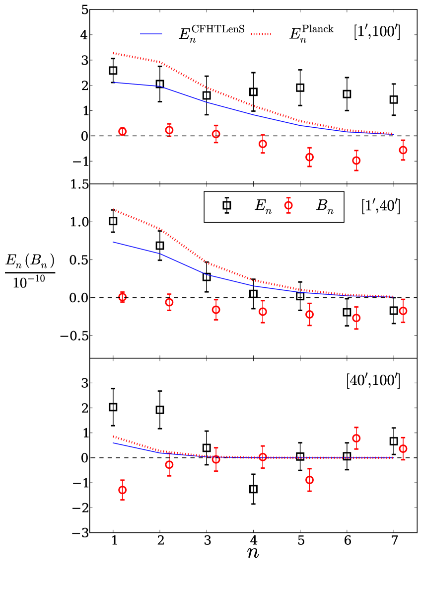
Fig. 1 shows the measured COSEBIs for a single redshift bin using all galaxies. The panels show the results for the three angular ranges, , and . The symbols show the COSEBIs modes estimated from the data while the theory values are shown as curves. The COSEBIs modes are discrete and the curves are drawn to aid the viewer. The E-mode COSEBIs are shown by black squares while the red circles are the B-modes. The B-modes are shifted to the right to aid the viewer. The errors on the data are estimated from the simulations and are correlated (see the covariance in Fig. 7). As we will see in Sect. 3.5, the B-modes in this plot are only significant for the angular scale . The theory E-mode curves belong to CFHTLenS+WMAP7 and Planck best fit values listed in Table 2. We also see that the highest signal-to-noise ratio comes from small scales as expected (see Asgari et al., 2012, for example).
|
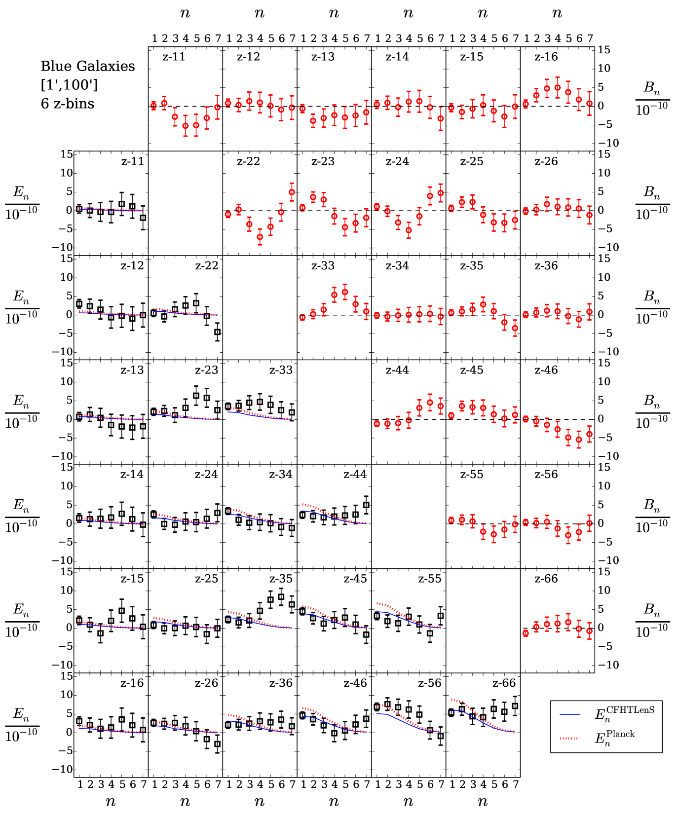
Fig. 2 shows the estimated COSEBIs for the tomographic case with blue galaxies. The E/B-modes are separated into the upper and lower triangle of the plot. Each panel belongs to a redshift bin pair indicated at its corner. Similar to Fig. 1 the measured E and B-modes are shown as black squares and red circles, respectively. The curves show the theory values of the E-modes for the CFHTLenS+WMAP7 and Planck cosmologies in Table 2. The angular range considered is . Unlike the single redshift bin case, we see statistically non-zero B-modes in this Figure.
|
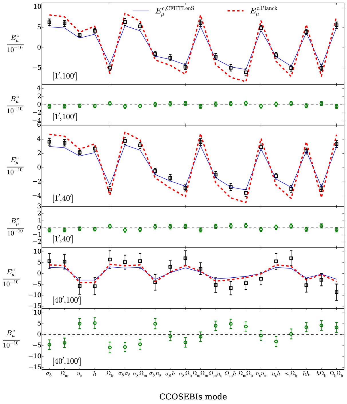
Fig. 3 shows the first measurement of CCOSEBIs from data. We use blue galaxies with 6 tomographic bins and the three angular ranges to estimate the CCOSEBIs. Here we choose the 5 cosmological parameters in Table 2 to compress COSEBIs into 5 first order and 15 second order CCOSEBIs, using the Planck values as our fiducial cosmology to calculate the compression matrix (see Eq. 10). The CCOSEBIs modes are named after the parameters which are used to define them, shown on the x-axis. The first order modes only depend on one cosmological parameter, whereas, the second order CCOSEBIs depend on two parameters which could be the same. For example, the points related to show the value of the second order CCOSEBIs mode which is based on the derivatives of COSEBIs to and . The ordering of the modes is arbitrary and the apparent oscillations in the figure can be rearranged. The theory values of the CCOSEBIs for CFHTLenS+WMAP7 and Planck cosmologies are shown as the blue solid curve and the red dashed curve. Note that the CCOSEBIs modes are discrete and the theory values are connected for an easier comparison. The B-modes are shown on the same scale as the E-modes. The CCOSEBIs are designed to be sensitive to cosmological information about these parameters. Therefore, they may not be as sensitive to the B-modes in the data. As we will see for most cases that we have studied, even if there are significant B-modes picked up by COSEBIs, the B-modes are not always significant with the CCOSEBIs. The exception is the angular range which shows significant B-modes either way.
|
3.5 Figure-of-merit and fitting
To quantify the significance of the measured B-modes we estimate their value with zero,
| (16) |
where is a vector composed of , is its transpose and is the inverse of the B-mode covariance matrix, estimated from the SLICS simulations. We also estimate the values for the E-modes compared to the best fit values of CFHTLenS+WMAP7 and Planck (see Table 2). The raw value of the is not particularly informative, even when the degrees-of-freedom is known (see Andrae et al., 2010, for example). Hence instead we show the p-values for the estimated values. The p-value shows the probability of finding a value larger than the one estimated. We choose a significance level of , p-value=0.01, which corresponds to a deviation of about for a normal distribution. Recall that a distribution is skewed towards smaller values and asymptotically reaches a normal distribution for large numbers of degrees-of-freedom as illustrated in Fig. 10. Additionally, using an inverted noisy covariance changes a distribution and hence the derived p-values, which we account for using the method proposed by Sellentin & Heavens (2015).
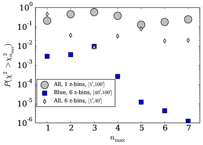
Fig. 4 shows the p-values for the COSEBIs versus , the maximum number of COSEBIs used starting from the first mode. The p-values are shown for the three configurations which are closest to the previous CFHTLenS analysis described in Sect. 3.1. The grey circles correspond to range without tomography and with all galaxies, which resembles Kilbinger et al. (2013). The blue squares belong to angular range with tomography and blue galaxies similar to Kitching et al. (2014). The diamonds configuration is the same as Heymans et al. (2013), where all galaxies in the angular range are considered and binned in redshift. In this plot we see that the p-values for the single redshift bin case are always above which means that they are insignificant. In contrast, on large scales the B-modes are always below and are significant. In addition, the tomographic analysis using the lower angular range, , also shows insignificant Bmodes with a p-value above . When we use CCOSEBIs the B-modes significance decreases, as we will see in Table 3.
|
Table 3 shows the p-values for all the cases that we have considered. The first four columns indicate the set-up, while the last six show the p-values for that set-up for, , , , , and , respectively. The p-values for CCOSEBIs are only shown for the tomographic cases where CCOSEBIs offers a compression. The column shows the number of COSEBIs modes in each redshift bin which are used in the analysis. We show the results for both the first 2 and 7 COSEBIs. The p-values are written in boldface where they are larger than which corresponds to the significance level within . Looking at the column and the single redshift bin cases, we see that the B-modes are only significant at large scales (). When redshift binning is considered, with the exception of the case there are significant B-modes in the data. The B-modes are not always consistent between the two galaxy populations which hints at a correlation between galaxy colour and residual systematics. Also notice that the largest scales show significant B-modes for all the different sets of data analysed.
The column shows the CCOSEBIs B-modes which are typically less significant than that of COSEBIs. As discussed before, this is due to the fact that the CCOSEBIs are based on linear combinations of COSEBIs which are most sensitive to cosmological parameters. They are therefore not necessarily sensitive to the B-modes which, for CFHTLenS, appear to cancel to some degree with the compressed form of the statistic. Consequently, to measure B-modes we need to use COSEBIs, which provide a complete set of functions for this analysis.
Comparing the and columns we see that Planck provides a better match to the single redshift bin data for all the cases666 Here we use p-values as a proxy for values, which would be used in sampling the parameter likelihood in a typical cosmological analysis. We will not attempt to reject either or using this method or quantify their tension.. However, when tomography is considered the CFHTLenS cosmology provides a better match with the exception of the very large scales. For blue galaxies at the p-values for and are comparable. We also note that for many of the tomographic cases, neither provide a good match. When all galaxies are considered we need to add intrinsic alignment corrections to our model as was done in Heymans et al. (2013). However, for blue galaxies the contribution from intrinsic alignment is expected to be small, hence we expect and find a good fit to the CFHTLenS values.
COSEBIs CCOSEBIs range Galaxies z-bins All 1 2 7 6 2 7 Blue 1 2 7 6 2 7 All 1 2 7 6 2 7 Blue 1 2 7 6 2 7 All 1 2 7 6 2 7 Blue 1 2 7 6 2 7
3.6 Single Parameter Fit
We use a very simple parametrization to fit the theory to data, consisting of one free parameter. We find its best fit value by minimizing its value and the error to the fit corresponds to the parameter value at around the minimum . For the B-modes the single parameter model we use is a constant,
| (17) |
for COSEBIs and CCOSEBIs, respectively. For the E-modes the models are a constant, times the theory E-modes, with CFHTLenS+WMAP7 and Planck cosmologies. For COSEBIs these are
| (18) |
and
| (19) |
whereas for CCOSEBIs
| (20) |
and
| (21) |
are the two models. The best fit and error values for , , , , , are listed in Table 4. The format of this table is the same as Table 3. Null B-modes result in a statistically zero , however, a statistically zero is not a sufficient condition for B-modes to be zero. The rows for which the COSEBIs B-modes are consistent with zero from the p-value test are shown in boldface. Some of the values which are consistent with zero in this table correspond to significant B-modes from the p-value test. This shows that the B-mode pattern in the data is not always well-modelled by a constant value.
COSEBIs CCOSEBIs range Galaxies z-bins All 1 2 7 6 2 7 Blue 1 2 7 6 2 7 All 1 2 7 6 2 7 Blue 1 2 7 6 2 7 All 1 2 7 6 2 7 Blue 1 2 7 6 2 7
3.7 Comparison to previous analyses
The Tables 3 and 4 allow us to compare our results with the previous CFHTLenS cosmic shear analysis. We first consider Heymans et al. (2012) who detail a systematics test using an E-B mode decomposition for three different two-point statistics; the top-hat shear variance, the 2PCF and the mass aperture statistics. Analysing angular scales from applying no redshift binning, they found no significant B-modes, which is consistent with our results.
Kilbinger et al. (2013) performed a two-dimensional analysis of the data using several cosmic shear methods, including the COSEBIs. The aim of their work was to use a large angular range to estimate cosmological parameters, but they faced difficulties estimating the COSEBIs from their mock data, known as the Clone simulations. The main reason for their difficulties was the fact that the accuracy of the simulations for very large angular scales is limited, due to the finite box size. Consequently, they did not use COSEBIs for their final analysis of the data. Here we used updated simulations (SLICS) with better accuracy for large scales and did not encounter similar problems. We compare their results with our angular range with all galaxies and a single redshift bin. They reported insignificant B-modes which is consistent with our results.
Kitching et al. (2014) restricted their study to large scales and blue galaxies with redshift information. They reported no significant B-modes. Although the scales they used are defined in Fourier space where they performed their analysis, they roughly correspond to the large scales that we have considered here. In contrast to their study we find very significant B-modes in the range. One reason for this inconsistency could be that their mask model lacks the precision to find the B-modes (see Asgari et al., 2016, for mask modelling). In contrast to power spectrum analysis, mask modelling has little or no effect on the estimation of COSEBIs. Alternatively, this inconsistency could be due to the complexity of translating the angular ranges used in a COSEBIs analysis to the Fourier modes considered in 3D-lensing.
Our best fit CFHTLenS+WMAP7 fiducial cosmology comes from Heymans et al. (2013), who used the range with tomography. They did not incorporate any E/B-mode decomposition methods in their analysis since they used 2PCFs to find their best fitting values. For the angular range they used, we find significant B-modes when all galaxies and 7 COSEBIs modes are considered. When only 2 COSEBIs modes are considered, or only using blue galaxies, the B-modes are consistent with zero. Considering blue galaxies only where intrinsic alignments are not important, we see that our measurements favour their best fit values in comparison to Planck. In particular, the CCOSEBIs matches to both theoretical values for this case, however the CFHTLenS+WMAP7 is a better match, as expected. Aside from our choice of observables and the modelling of the intrinsic alignments, there are no other differences between our study and Heymans et al. (2013).
4 Conclusions
In this paper we revisited the CFHTLenS data and found evidence for systematic errors on large scales, and when the data is analysed in tomographic bins. We used COSEBIs, which is a robust efficient and complete method for E/B-mode separation. We expect weak lensing to predominantly produce E-modes, making B-modes undesirable. Although the absence of B-modes does not guarantee a perfect data analysis, it is a necessary condition for a survey like CFHTLenS. For future large scale and space based surveys, where the measurement errors are significantly smaller, the B-modes could also indicate other physical phenomena. For example we know that some intrinsic alignment models predict these modes (see Blazek et al., 2011, and references therein). Before performing our analysis we carried out a number of blind tests on cosmological simulations, to test the accuracy of our pipelines which are reported in the Appendix. The significance of the B-modes we found is highest for large scales, , especially when the galaxies are divided into redshift bins. They also depend on the galaxy population used in the analysis. We repeated our analysis for blue and all galaxies, since blue galaxies do not show a strong intrinsic alignment signal.
Our COSEBIs measurement on tomographic data is the first of its kind. Previously, all COSEBIs data analysis has been limited to 2D cosmic shear data. Dividing galaxies into different redshift bins tightens the constraints on cosmological parameters, as it adds information about structure evolution, which is essential for constraining dark energy parameters. Adding redshift information to data analysis increases the total number of COSEBIs that need to be measured. This makes covariance matrix estimations more challenging, since a larger number of simulations are needed to reach a satisfactory precision. To alleviate this we showed the first measurement of compressed COSEBIs (CCOSEBIs) which are composed of linear combinations of the COSEBIs that are most sensitive to cosmological information. This compression reduces the number of observables substantially. In this study where we used 7 COSEBIs modes and 6 redshift bins. The total number of 147 COSEBIs modes, reduced to 20 CCOSEBIs to estimate 5 cosmological parameters. As a result, the estimated covariance for the CCOSEBIs has a higher precision.
We analysed our data according to angular scale and galaxy type, as well as analysing the data with and without tomographic redshift bins. We considered different samples of galaxies to compare our results with previous cosmic shear analyses of the CFHTLenS data. Since our analysis focuses on tests for systematic errors, instead of parameter estimation, we compare our measurements to two different flat CDM cosmological models with Planck and CFHTLenS+WMAP7 best fit parameters. We calculated the goodness-of-fit of these two models to our data for the full range of analyses. The figure-of-merit used the p-value for a analysis, which indicates the probability of finding a value larger than the value found. We highlighted the values which corresponded to at least confidence. In addition, we used the same method to report the significance of the B-modes we found. We also used a simple parametrization to find the best fit values of a single parameter to our data. We find consistent results with Heymans et al. (2013), with little or insignificant B-modes in range. Both COSEBIs and CCOSEBIs show a better match to CFHTLenS cosmology over Planck for this angular range with redshift binning.
We compared our large scale results with blue galaxies and tomography with Kitching et al. (2014), were we found the most significant B-mode signal, which is in tension with their finding of a zero B-mode. Our measured E-modes for this configuration show a slightly better match to Planck cosmology in agreement with Kitching et al. (2014). However, the cosmic shear information in this range is the lowest and as a result it has the weakest constraining power. On the other hand, as the modelling of baryons is associated with a rather large uncertainty, restricting the analysis to larger angular scales most likely removes systematics due to modelling.
Our results are in line with Kilbinger et al. (2013) who reported insignificant B-modes for a single redshift bin and a wide angular range with all galaxies. Our COSEBIs measurements in this range match with Planck cosmology better than CFHTLenS+WMAP7 which is also consistent with the parameter constraints from Kilbinger et al. (2013) which are in less tension with Planck than the tomographic CFHTLenS analysis.
Fu et al. (2014) have also reported B-modes in CFHTLenS for three-point statistics, using aperture mass statistics. Our results together show that there are remaining systematics left in the data. One hypothesis is that these systematics arise from selection effects which introduce a correlation between the PSF ellipticity and the galaxy ellipticity when galaxies are divided into redshift bins. The B-modes we measured are in general larger when tomography is considered. This will be investigated in more detail in our future work. Although not quantified here we can see an anti-correlation between the E-modes and B-modes which is visible in the plots. This suggests that the systematic errors affect the E/B-modes in the same way.
The CCOSEBIs show insignificant B-modes for many cases that we have studied, even when the COSEBIs indicate otherwise. Currently, we do not have a full understanding of how systematic errors affect E/B-modes. This can be investigated by simulating systematic errors that show a similar signature to the ones found here, and examine their effect on E-modes. Nevertheless, assuming that the systematic errors affect the two modes in the same way (as hinted by the E/B anti-correlation), we can conclude that for the cases where the CCOSEBIs B-modes are negligible, they are not degenerate with the cosmological parameters, which means that the B-modes detected by the COSEBIs should not bias the parameter estimations. Note that given the assumption above, if the CCOSEBIs modes are not sensitive to the systematics then they must be orthogonal to them.
The methods and pipelines used in this analysis can and should be used with any other reduced cosmic shear dataset. COSEBIs is arguably the best method for testing for B-modes in the data and can also be used for measuring B-modes for cosmological analysis. Future and ongoing surveys will suffer more from inaccuracies in their covariance estimations, which can be remedied by either using a larger number of simulations or by decreasing the number of data points used in the analysis. As N-body simulations are expensive and time consuming we recommend using the compression method in Asgari & Schneider (2015) applied to COSEBIs to find CCOSEBIs and accurate cosmological parameters.
Acknowledgements
MA and CH acknowledge support from the European Research Council through grant number 240185 and 647112. CB acknowledges the support of the Australian Research Council through the award of a Future Fellowship. PS is supported by the Deutsche Forschungsgemeinschaft under the program TR33 and SCHN-342/13. JHD acknowledges support from NSERC. Computations for the -body simulations were performed on the GPC supercomputer at the SciNet HPC Consortium. SciNet is funded by: the Canada Foundation for Innovation under the auspices of Compute Canada; the Government of Ontario; Ontario Research Fund - Research Excellence; and the University of Toronto. We thank the CFHTLenS team for making the data publicly available. This work is based on observations obtained with MegaPrime/MegaCam, a joint project of CFHT and CEA/IRFU, at the Canada-France-Hawaii Telescope (CFHT) which is operated by the National Research Council (NRC) of Canada, the Institut National des Sciences de l’Univers of the Centre National de la Recherche Scientifique (CNRS) of France, and the University of Hawaii. This research used the facilities of the Canadian Astronomy Data Centre operated by the National Research Council of Canada with the support of the Canadian Space Agency. CFHTLenS data processing was made possible thanks to significant computing support from the NSERC Research Tools and Instruments grant program.
References
- Addison et al. (2016) Addison G. E., Huang Y., Watts D. J., Bennett C. L., Halpern M., Hinshaw G., Weiland J. L., 2016, ApJ, 818, 132
- Andrae et al. (2010) Andrae R., Schulze-Hartung T., Melchior P., 2010, preprint, (arXiv:1012.3754)
- Asgari & Schneider (2015) Asgari M., Schneider P., 2015, A&A, 578, A50
- Asgari et al. (2012) Asgari M., Schneider P., Simon P., 2012, A&A, 542, A122
- Asgari et al. (2016) Asgari M., Taylor A., Joachimi B., Kitching T. D., 2016, preprint, (arXiv:1612.04664)
- Bartelmann & Schneider (2001) Bartelmann M., Schneider P., 2001, Phys. Rep., 340, 291
- Battye & Moss (2014) Battye R. A., Moss A., 2014, Physical Review Letters, 112, 051303
- Becker et al. (2015) Becker M. R., et al., 2015, preprint, (arXiv:1507.05598)
- Benjamin et al. (2013) Benjamin J., et al., 2013, MNRAS, 431, 1547
- Blazek et al. (2011) Blazek J., McQuinn M., Seljak U., 2011, J. Cosmology Astropart. Phys., 5, 10
- Bond & Efstathiou (1984) Bond J. R., Efstathiou G., 1984, ApJ, 285, L45
- Choi et al. (2015) Choi A., et al., 2015, preprint, (arXiv:1512.03626)
- Dossett et al. (2015) Dossett J. N., Ishak M., Parkinson D., Davis T. M., 2015, Phys. Rev. D, 92, 023003
- Eifler (2011) Eifler T., 2011, MNRAS, 418, 536
- Erben et al. (2013) Erben T., et al., 2013, MNRAS, 433, 2545
- Fu & Kilbinger (2010) Fu L., Kilbinger M., 2010, MNRAS, 401, 1264
- Fu et al. (2014) Fu L., et al., 2014, MNRAS, 441, 2725
- Harnois-Déraps & van Waerbeke (2015) Harnois-Déraps J., van Waerbeke L., 2015, MNRAS, 450, 2857
- Harnois-Déraps et al. (2015) Harnois-Déraps J., van Waerbeke L., Viola M., Heymans C., 2015, MNRAS, 450, 1212
- Hartlap et al. (2007) Hartlap J., Simon P., Schneider P., 2007, A&A, 464, 399
- Heymans et al. (2012) Heymans C., et al., 2012, MNRAS, 427, 146
- Heymans et al. (2013) Heymans C., et al., 2013, MNRAS, 432, 2433
- Hilbert et al. (2009) Hilbert S., Hartlap J., White S. D. M., Schneider P., 2009, A&A, 499, 31
- Hildebrandt et al. (2012) Hildebrandt H., et al., 2012, MNRAS, 421, 2355
- Huff et al. (2014) Huff E. M., Eifler T., Hirata C. M., Mandelbaum R., Schlegel D., Seljak U., 2014, MNRAS, 440, 1322
- Joachimi & Schneider (2008) Joachimi B., Schneider P., 2008, A&A, 488, 829
- Joudaki et al. (2016) Joudaki S., et al., 2016, preprint (arXiv:in prep)
- Kilbinger (2015) Kilbinger M., 2015, Reports on Progress in Physics, 78, 086901
- Kilbinger et al. (2013) Kilbinger M., et al., 2013, MNRAS, 430, 2200
- Kilbinger et al. (2014) Kilbinger M., Bonnett C., Coupon J., 2014, athena: Tree code for second-order correlation functions, Astrophysics Source Code Library (ascl:1402.026)
- Kitching et al. (2014) Kitching T. D., et al., 2014, MNRAS, 442, 1326
- Köhlinger et al. (2015) Köhlinger F., Viola M., Valkenburg W., Joachimi B., Hoekstra H., Kuijken K., 2015, preprint, (arXiv:1509.04071)
- Kuijken et al. (2015) Kuijken K., et al., 2015, MNRAS, 454, 3500
- Laureijs et al. (2011) Laureijs R., et al., 2011, ArXiv:1110.3193,
- MacCrann et al. (2015) MacCrann N., Zuntz J., Bridle S., Jain B., Becker M. R., 2015, MNRAS, 451, 2877
- Mead et al. (2015) Mead A. J., Peacock J. A., Heymans C., Joudaki S., Heavens A. F., 2015, MNRAS, 454, 1958
- Melchior & Viola (2012) Melchior P., Viola M., 2012, MNRAS, 424, 2757
- Miller et al. (2013) Miller L., et al., 2013, MNRAS, 429, 2858
- Planck Collaboration et al. (2015a) Planck Collaboration et al., 2015a, preprint, (arXiv:1502.01589)
- Planck Collaboration et al. (2015b) Planck Collaboration et al., 2015b, preprint, (arXiv:1502.01590)
- Press et al. (2002) Press W. H., Teukolsky S. A., Vetterling W. T., Flannery B. P., 2002, Numerical Recipes in C++. Cambridge University Press
- Raveri (2015) Raveri M., 2015, preprint, (arXiv:1510.00688)
- Schneider & Kilbinger (2007) Schneider P., Kilbinger M., 2007, A&A, 462, 841
- Schneider et al. (1998) Schneider P., van Waerbeke L., Jain B., Kruse G., 1998, MNRAS, 296, 873
- Schneider et al. (2002) Schneider P., van Waerbeke L., Mellier Y., 2002, A&A, 389, 729
- Schneider et al. (2010) Schneider P., Eifler T., Krause E., 2010, A&A, 520, A116
- Sellentin & Heavens (2015) Sellentin E., Heavens A. F., 2015, preprint, (arXiv:1511.05969)
- Semboloni et al. (2011) Semboloni E., Hoekstra H., Schaye J., van Daalen M. P., McCarthy I. G., 2011, MNRAS, 417, 2020
- Semboloni et al. (2013) Semboloni E., Hoekstra H., Schaye J., 2013, MNRAS, 434, 148
- Simpson et al. (2013) Simpson F., et al., 2013, MNRAS, 429, 2249
- Smith et al. (2003) Smith R. E., et al., 2003, MNRAS, 341, 1311
- Spergel et al. (2015) Spergel D. N., Flauger R., Hložek R., 2015, Phys. Rev. D, 91, 023518
- Takahashi et al. (2012) Takahashi R., Sato M., Nishimichi T., Taruya A., Oguri M., 2012, ApJ, 761, 152
- Taylor & Joachimi (2014) Taylor A., Joachimi B., 2014, MNRAS, 442, 2728
- The Dark Energy Survey Collaboration et al. (2015) The Dark Energy Survey Collaboration et al., 2015, preprint, (arXiv:1507.05552)
- Velander et al. (2014) Velander M., et al., 2014, MNRAS, 437, 2111
- Verde et al. (2013) Verde L., Feeney S. M., Mortlock D. J., Peiris H. V., 2013, J. Cosmology Astropart. Phys., 9, 13
Appendix A Pipeline Optimization and Verification
In this Appendix we present a series of tests to explore the effects of noise and discrete integration on the determination of the COSEBIs for CFHTLenS-like data.
A.1 Power spectra vs. 2PCFs
|
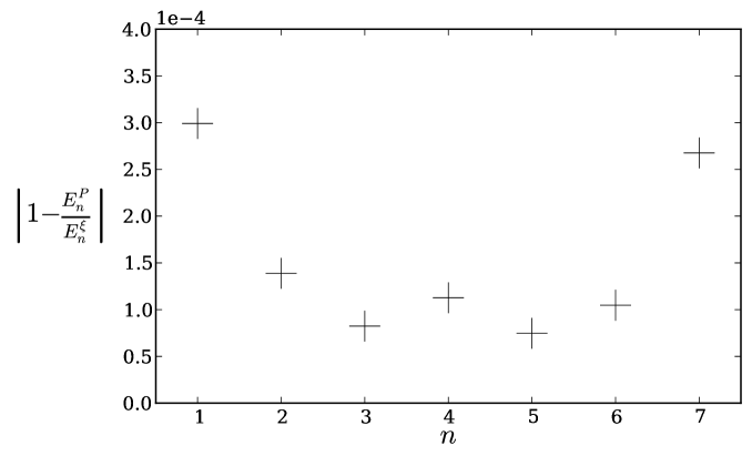
In Asgari et al. (2012) we calculated COSEBIs numerically, assuming a perfect knowledge, i.e. a noise-free measurement, of the input quantities. We used Eq. (6) to find the E-mode COSEBIs which is more convenient to use for a theoretical analysis, since most theories provide us with an input power spectrum. However, in practice shear 2PCFs are more straightforward to measure, from which COSEBIs can then be inferred via Eq. (4). The first test therefore checks if the two equations Eq. (6) and Eq. (4) result in the same when calculated numerically assuming noise-free data. For this test we choose an angular range of . Fig. 5 shows the residual ratio of numerically calculated from Eq. (6) and Eq. (4) for . As we can see in this figure, the values of from the two methods agree to better than . Figure 10 of Asgari et al. (2012) shows the dependence of three cosmological parameters to the first 5 COSEBIs. From this figure we conclude that the small difference between from Eq. (6) and Eq. (4) is therefore indeed insignificant for our analysis (for example, if changes by then will change by about ).
A.2 From Smooth Integration to Noisy Trapezoidal
In Appendix. A.1 we assumed a perfect knowledge of the 2PCFs over the angular range considered, a Gaussian integration method (see Press et al., 2002) between two extrema of the integrand is employed to evaluate in both cases. In practice, however, we only have the values of 2PCFs in angular bins or at certain values. Consequently, we need to use a different integration routine to evaluate from Eq. (4) for real data. The most straightforward integration method is the trapezoidal method for a linearly binned data. In this section we determine how many linear angular bins are needed to reach a certain accuracy in determining .
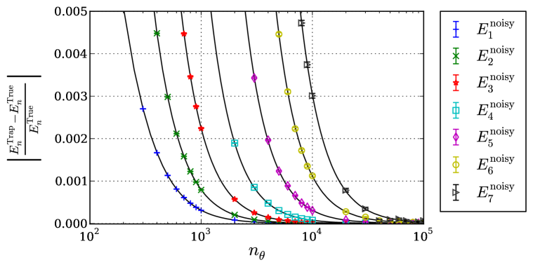
The solid curves in Fig. 6 show the fractional deviation of as a function of angular bins used in the trapezoidal integration assuming noise-free data. All the values are normalized by their true value, calculated from the convergence power spectrum using Eq. (6). As can be seen in Fig. 6 a larger number of angular bins are required for the higher COSEBIs modes, to reach the same accuracy. The reason for this behaviour is that, the functions have roots in their range of support and oscillate around them. Consequently, the higher modes are more sensitive to the number of bins incorporated in their integral (see Schneider et al., 2010; Asgari et al., 2012). Following Fig. 10 in Asgari et al. (2012) we choose an accuracy of for which corresponds to an accuracy on of . This enforces a lower limit of 10000 bins for, , the highest COSEBIs mode we use in this analysis.
|
We next include the effects of noise on the estimated . Since the number of bins needed to reach the accuracy desired is high, the shot noise term of the correlation function covariance dominates the other terms in this case. We will therefore choose to ignore other sources of noise for this test, using only the shot noise in the covariance, at this stage. We can make a noisy mock data set from
| (22) |
where
| (23) |
is the square root of the shot noise term in the 2PCFs covariance (see Joachimi & Schneider, 2008, for example), with , the intrinsic ellipticity dispersion of the galaxies, deg2, the area of the survey, arcmin2, the effective mean number density of galaxies and the width of the angular bins. is a randomly generated number from a Gaussian distribution with a variance of 1 and a mean of 0. With the above definitions the covariance of is equal to the desired covariance. The symbols in Fig. 6 show the ensemble average estimate of from 50 realizations with respect to the number of angular bins. The errors shown are the standard deviation of the mean value of over all the realizations. The presence of the random errors do not change the conclusions drawn from the previous test. By comparing the curves and the symbols in Fig. 6 we can also conclude that the random noise due to the intrinsic ellipticity dispersion of galaxies does not bias the estimation of COSEBIs.
|
|
|
A.3 Simulations: Covariance Matrix Estimation
In this section we determine COSEBIs on the mock data from the SLICS simulations which resemble the CFHTLenS data. Here we also show the covariance matrices which are used in the main analysis and are estimated from the simulated data. In this paper we use the second version of the CFHTLenS CLONE catalogue777The first version is available on www.cfhtlens.org, which is based on the SLICS N-body simulations (see Harnois-Déraps & van Waerbeke, 2015, for details) and consist of 497 independent lines of sight, 60 square degrees each. These mock catalogues are specifically made for the CFHTLenS data, taking into account its redshift distribution. Furthermore, source clustering effects are included in these catalogues. The limited box size of the simulations dictates the maximum scale that can be trusted. In addition, the resolution of the simulations put limits on the small scales. Combining this with the fact that on small scales baryonic effects (not included in the simulations) become important, we limit our minimum angular range as well (see Semboloni et al., 2011, for the effects different baryon feedback models have on structure formation and ). Hence, we choose to only use scales in in our analysis.
Since the simulated covariance is different from the Gaussian random noise we used in Appendix. A.2 we repeat the angular bin versus measured test using the simulated data. The covariance of the COSEBIs is defined as,
| (24) |
where is the expectation value of . The covariance is estimated from the simulations via,
| (25) |
where
| (26) |
is the mean over all lines-of-sight of the simulated fields.
We find similar conclusions from repeating the bin size exercise. Nevertheless, for the rest of the analysis we choose to use linear bins in , which is larger than the threshold we found in the previous section. With a narrower angular binning scheme the number of galaxies in each bin decreases. Hence the estimate is noisier. In this analysis we have made sure that all the bins are populated with galaxies. Increasing the number of 2PCFs angular bins cannot reduce the accuracy of the estimated COSEBIs, as long as all the angular bins are populated with pairs of galaxies.
|
|
|
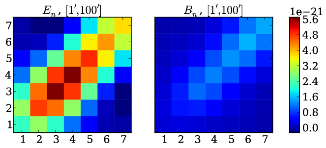
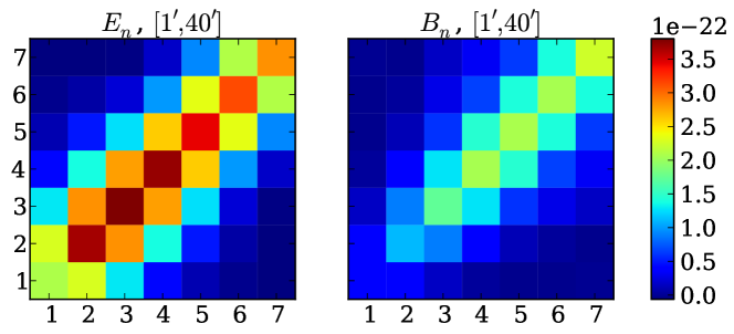
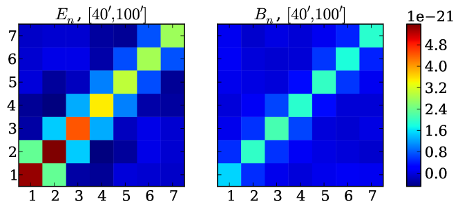
The COSEBIs covariance for a single redshift distribution from the simulations is shown in Fig. 7, for the three angular ranges , and . The right panels show the covariance for while the left panels show the same for . All the covariances are scaled by a factor of to correspond to the effective CFHTLenS area, where we have 497 mock fields, 60 deg2 each. The effective area of CFHTLenS passed fields is 94.564 deg2.
In the simulated catalogues a mock best fit value of each galaxy’s redshift, , is given, which is in general different from its spectroscopic value. To mimic the real data we use to choose which redshift bin a galaxy belongs to. Whilst tomographic bins have no overlap in , this is not the case for the underlying true redshift distribution.
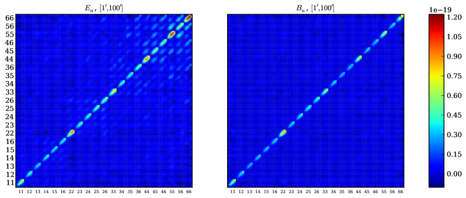
Fig. 8 shows the covariance matrices for with the six redshift bins in Table 1. Each block in the covariance matrix has elements corresponding to a combination of redshift bin pairs. The x/y-axis in the plots show the redshift bin pairs considered. In total the covariance has elements. The left and right panels show the covariance matrix for the and , respectively. In Fig. 8 we see that for all cases, the value of the covariance drops for the off-diagonal elements. Although not shown here for the tomographic case, for both redshift binning cases the range has a more diagonal covariance. This is due to the fact that non-Gaussian effects are less important for this angular range. Therefore, any analysis which only uses this angular range is less likely to be biased because of poor modelling of non-linear scales. However, the cosmic shear information in this angular range is significantly lower than that of the lower angular scales.
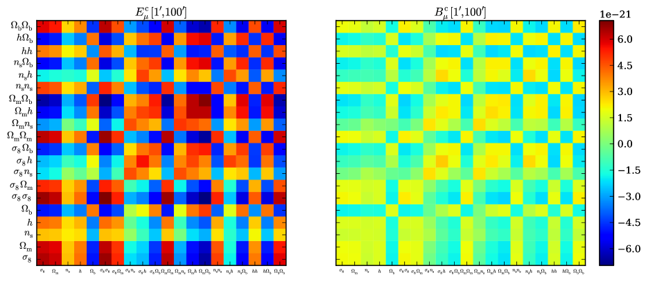
Fig. 9 shows the covariance matrices for the E-mode and B-mode CCOSEBIs for six redshift bins and , measured from the SLICS simulations. The x-/y-axis show the CCOSEBIs modes for which the covariance is shown. In this work we chose five cosmological parameters, , , , and . This means that we have 5 first order CCOSEBIs which depend on the covariance and the first order derivatives of the COSEBIs with respect to the parameters, and 15 second order CCOSEBIs which depend on the covariance and the second order derivatives of the COSEBIs with respect to the parameters. Hence we show the CCOSEBIs modes by the parameters with respect to which the compression is made. In total for 5 parameters there are 20 CCOSEBIs modes irrespective of the number of redshift bins. Hence, for the case of 6 redshift bins we have compressed 147 parameters to only 20 and reduced the size of the covariance substantially, as can be seen by comparing Fig. 8 and Fig. 9. The cross-covariance between the CCOSEBIs modes is relatively high for some of the cases. This is due to the fact that the CCOSEBIs modes are based on cosmological parameters which can have large degeneracies. For example, the and which have a large degeneracy in cosmic shear analysis, also show a large cross-covariance.
A.4 B and E-mode analysis of mocks
The simulated mock catalogues should be B-mode free, providing an opportunity to explore how random ellipticity noise can affect the measured B-modes. For each line-of-sight we measure all values and determine the values for ,
| (27) |
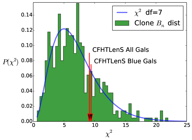
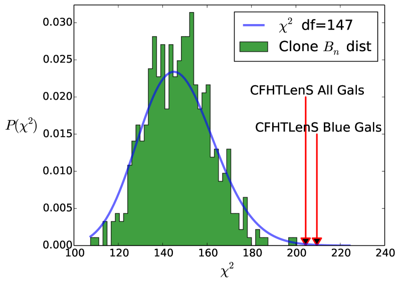
where is the vector and is the covariance matrix of . Fig. 10 shows the distribution of the for the 497 SLICS simulations (green histograms). The left panel belong to the single redshift case, whereas the tomographic case is shown in the right panel. Since, in this study we used 7 COSEBIs modes the degrees-of-freedom for the single redshift bin case is 7, while for the tomographic case it is 147. The blue solid curves show the theoretical distribution for a given degrees-of-freedom, and they match the histograms888We checked this using a Kolmogorov–Smirnov test.. Consequently, we conclude that the B-modes in the simulations are statistically consistent with zero and provide a distribution with which to compare the real data. The red arrows show the value of the B-modes corresponding to the CFHTLenS data with . We can see that the blue galaxies show a more significant B-mode signal compared to all galaxies. Furthermore, the values of the CFHTLenS data for the tomographic case are well beyond what is expected from the simulations. We also calculated the CCOSEBIs from the simulations and confirmed that they follow a distribution with 20 degrees-of-freedom.
The E-mode COSEBIs were also optimized and tested using the same set of catalogues. We performed a blind analysis of the mocks to test if the input cosmology of the simulations can be recovered. The distributions for the , where is estimated from the simulations and is its expected theory value, is very similar to the distributions of the (Fig. 10), hence we do not show them here. The CFHTLenS data analysis was then carried out without any changes to the pipelines.
Appendix B values and degrees-of-freedom
Comparing raw values can be misleading for two reasons: firstly a distribution is asummetric and secondly this distribution highly depends on the degrees-of-freedom associated with the value. However, in Table 5 we provide the degrees-of-freedom for each element in Table 3 and the values to give the readers the opportunity to perform their own interpretation of the data.
COSEBIs CCOSEBIs range Galaxies z-bins DOF DOF DOF DOF DOF DOF All 1 2 7 6 2 7 Blue 1 2 7 6 2 7 All 1 2 7 6 2 7 Blue 1 2 7 6 2 7 All 1 2 7 6 2 7 Blue 1 2 7 6 2 7