3-—\CF@arrow@shift@nodes#3\draw[-—](\CF@arrow@start@node)–(\CF@arrow@end@node);\CF@arrow@display@label#10.5+\CF@arrow@start@node#20.5-\CF@arrow@end@node \definearrow1s¿\CF@expadd@tocsshorten ¡=\CF@arrow@offset,shorten ¿=\CF@arrow@offset,\CF@arrow@current@style\draw[shorten ¡=\CF@arrow@offset,shorten ¿=\CF@arrow@offset,,-CF@full](\CF@arrow@start@name)..controls#1..(\CF@arrow@end@name); \definearrow1s¡¿\CF@expadd@tocsshorten ¡=\CF@arrow@offset,shorten ¿=\CF@arrow@offset,\CF@arrow@current@style\draw[shorten ¡=\CF@arrow@offset,shorten ¿=\CF@arrow@offset,,CF@full-CF@full](\CF@arrow@start@name)..controls#1..(\CF@arrow@end@name);
Precision and Sensitivity in Detailed-Balance Reaction Networks
Abstract.
We study two specific measures of quality of chemical reaction networks, Precision and Sensitivity. The two measures arise in the study of sensory adaptation, in which the reaction network is viewed as an input-output system. Given a step change in input, Sensitivity is a measure of the magnitude of the response, while Precision is a measure of the degree to which the system returns to its original output for large time. High values of both are necessary for high-quality adaptation.
We focus on reaction networks without dissipation, which we interpret as detailed-balance, mass-action networks. We give various upper and lower bounds on the optimal values of Sensitivity and Precision, characterized in terms of the stoichiometry, by using a combination of ideas from matroid theory and differential-equation theory.
Among other results, we show that this class of non-dissipative systems contains networks with arbitrarily high values of both Sensitivity and Precision. This good performance does come at a cost, however, since certain ratios of concentrations need to be large, the network has to be extensive, or the network should show strongly different time scales.
Key words. Sensory adaptation, reaction network, dissipation, matroid.
1. Introduction
1.1. Dissipation and adaptation
It has been known at least since Szilard [Szi29] and Landauer [Lan61] that practical information processing requires the dissipation of free energy. In recent years interest has arisen in the application of this idea to chemical and biochemical systems, and studies have been made of the role of dissipation in decision making [QR05], concentration sensing [Tu08, MS12, SNMW13, GtW13], signal transduction [LHW08, BS13], behaviour of oscillators [WXW08, XZWW13, CWOT15], error correction [MHL12], sensory adaptation [LSN+12, LT13, SGLH14, Lan15, BDGC15], and various others.
A common theme in these works is a focus on the relationship between the quality of the processing on one hand and the magnitude of the dissipation on the other; in most cases the conclusion is that dissipation ‘improves the situation’, in the sense of leading to higher accuracy, speed, or reliability. However, much of the current literature is based on single examples, in which simplified models are studied, and often the tuning of the amount of dissipation amounts to a single scalar parameter.
In fact, given an arbitrary chemical reaction system, there appear to be multiple definitions of the ‘amount of dissipation’ at a given parameter point, which differ in whether they apply only to a stationary point or also to dynamic states, whether they include stochastic fluctuations, and whether they operate at a macroscopic or a microscopic level. This makes it difficult to compare results and make clear statements.
As a first step towards such clear statements, in this paper we approach the problem from the other end: we consider dissipation-free systems, and ask the question to which extent these can or can not process information. We do this with the information-processing example of sensory adaptation.
Adaptation is best explained with the example of the bacterium E. coli. As part of its food-finding strategy, E. coli propels itself in a straight line through its environment, while monitoring the concentration of e.g. glucose outside the cell. Depending on whether this concentration increases or decreases during this ‘run’, it will continue to move for longer or shorter in that direction; upon stopping, it turns to a random new direction, and starts a new run. This stochastic motion has a bias in the direction of increasing concentration, and this is how the bacterium finds its food.
In order to behave in this way, the bacterium has to convert small changes in concentration (a few percent up or down) into large changes in behaviour: ie. it has to show large Sensitivity, in the terminology that we define below. At the same time the sensing mechanism has to ‘reset’ or ‘zero itself’ after such a change, in order to be ready for the next change in concentration: a simplified version of this will be called Precision below. Most chemical reaction systems do not show this combination of Sensitivity and Precision, but when they do, we call them adaptive.
In this paper we study such adaptive systems, and more precisely, we ask the question
Q. To which extent can a non-dissipative system perform such adaptation?
This question is not only inspired by the general link between dissipation and functionality, already mentioned above. In recent work, Lan, Tu, and co-authors conclude that adaptive systems are necessarily dissipative [LSN+12, LT13]. If that is the case, then the answer to the question above should be ‘not at all’.
In fact, the situation turns out to be different, and surprising: we will see that a non-dissipative system is in fact perfectly capable of adaptation, in the sense that Sensitivity and Precision can both be arbitrarily high. However, there are strong limitations, as we shall also see: such good performance requires an extreme setup, in the sense that (a) certain ratios of steady-state concentrations have to be large, (b) time-scale separation has to be significant, or (c) large networks are required.
1.2. Content of this paper
In order to discuss what ‘non-dissipative’ systems can or can not do, one needs a proper definition of this class of systems. In this paper we define ‘non-dissipative’ systems as chemical reaction networks with mass-action kinetics satisfying detailed balance. This is a delicate issue, however, and we discuss it in more detail in Section 7.
Given this class, question Q above asks for the ‘most adaptive’ behaviour that such a system can perform. To structure this discussion, we will consider the structure of the network—the stoichiometry—to be given, and ask to which extent variation of the kinetic parameters allows the system to have large Precision and Sensitivity (which we define below).
We start the development in Section 2 by defining the various objects and concepts. In Section 3 we investigate the Precision, and specifically prove bounds on the minimal Precision, or maximal inverse Precision. Although we are interested in systems with large Precision, not small Precision, the concept of maximal inverse Precision plays a role in the study of Sensitivity in Section 4. There we show that we can make systems with large Precision and Sensitivity, by choosing the stoichiometry and the kinetic parameters in the right way.
The proof of Theorem 3.2, a combinatorial characterization of minimal Precision, is inspired by matroid theory, and in Section 5 we explain this connection. In Section 6 we give an example of a dissipative system with high Sensitivity and Precision that is small and has only moderate concentration ratios. We conclude with a discussion of the results.
2. Setup
In this section we give mathematical definitions of the objects that we will be considering.
2.1. Chemical reaction networks
A chemical reaction network is a set of reactions between chemical species , ,
Here and are the stoichiometric coefficients, which we assume to be non-negative numbers. This leads to the following definition.
Definition 2.1 (Systems).
A system is a triple , where
-
•
is a finite set of species;
-
•
is a finite set of reactions;
-
•
, , is a stoichiometric matrix, an matrix of real numbers such that is the relative increase or decrease of species under reaction .
A kinetic system is a quadruple , where is a function that gives, for each set of concentrations of the species, and for each reaction , the net rate of transformation in that reaction.
For any kinetic system, the evolution of the concentrations of the species is given by the ordinary differential equation111All quantities in this paper can be considered dimensionless, if necessary by non-dimensionalization against standard SI units.
| (1) |
Example 2.1. Consider the following reactions between species , , and :
For this system the species set is , the reaction set is ; the stoichiometric matrix and the kinetic function are
The dynamics of this reaction network is described by the ODE (1), which reads for this system
| (2) |
time [t] at 245 2
\pinlabel
concentration
[r] at 2 180
\endlabellist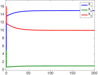 \labellist\pinlabeltime [t] at 245 10
\pinlabel
concentration
[r] at 2 180
\endlabellist
2.2. Mass-action and detailed balance
Definition 2.2 (Mass-action, detailed-balance kinetics).
Given a system , mass-action detailed-balance kinetics is given by functions of the form222Mass-action kinetics are of the form and the structure (3) follows from the detailed-balance assumption that there exists a stationary state at which all reactions are in equilibrium. See e.g. [ÉT89].
| (3) |
where we write for the column vector of and corresponding to reaction , and the notation stands for the monomial . The function (3) is characterized by the parameters .
We often write 333This 4-tuple does not completely determine and , only , and therefore does not contain enough information to characterize the full kinetics (3). The linearization of (3) at a stationary point only depends on , however, and since the Sensitivity and Precision are defined in terms of this linearization, this contains the necessary information for our purposes. for the kinetic system generated by this pair . Note that is a stationary point for (3), but there typically are other stationary points. This is related to the fact that when is a strict subspace of , then the evolution (1) takes place in a subset, a simplex:
Definition 2.3 (Stoichiometric simplex).
Let . For any , the stoichiometric simplex is the relatively open simplex
The stoichiometric simplex is the set of positive concentrations that can be reached by starting from and assigning arbitrary rates to each of the reactions. It is invariant under the evolution (1).
Example 2.1 (continued). For Example 2.1, the range of is the set , implying that the ODE (2) admits the conservation law . Consequently, the stoichiometric simplices are the sets
Lemma 2.4 (Stationary states).
For given , there exists exactly one stationary point of (1) in each simplex , and each solution in converges to it for large time. We indicate this stationary point by . The mapping is a smooth mapping from to ; is the unique solution of the equations
| (4) |
Proof.
The existence, uniqueness, and attraction properties are well-known in the field of chemical reaction theory; see e.g. [HJ72, Th. 6A]. The equation (4) can be verified by inspecting (3) or by using the fact that free energy decreases along a solution [HJ72, MM]. Finally, the smooth dependence follows from applying the implicit function theorem to (4). ∎
Remark 2.5 (Modifying ).
Below we will consider systems described by parameters , and concentrate on linearizations at some stationary point , which a priori need not be equal to . However, without loss of generality we can assume that the stationary point equals , by describing the same system by a new but equivalent set of parameters , where
The equations (1)-(3) are identical for and . We will therefore always assume that the stationary point under consideration is . ∎
Remark 2.6 (Independence of ).
As long as is a vector with strictly positive components, is independent of , as can be recognized from the absence of from (4). (If one of the components of vanishes, however, this amounts to removing a column from , which modifies (4) and leads to a different equation. We will use this idea below.) ∎
2.3. Precision and Sensitivity for detailed-balance reaction networks
We now think of a chemical reaction network as an input-output system, and we restrict ourselves to detailed-balance, mass-action kinetics networks. The input and output variables are concentrations, indicated by , .
The rest of this paper is based on the following setup.
The adaptation experiment. Prepare the system in a steady state ; at time zero, instantaneously add an amount of the input species to the system, thus increasing ; observe the evolution of the output variable (see Figure 2).
addition of [l] at 44 10
\pinlabeltime by -1.1 0 at 270 28
\pinlabelsmall when Precision is large [l] at 278 72
\pinlabel [l] at 489 94
\pinlabel [br] at 48 110
\endlabellist
In this situation, the Sensitivity is defined444This terminology follows [MTES+09]. Note however that the term ‘sensitivity’ also may refer to the variation of a stationary state under variation of a parameter, as in ‘parameter sensitivity’ [HS96] or more generally as the depedence of a model prediction on the assumptions and parameters [SRA+08]. as a normalized measure of the strength of the response of to the change in :
Definition 2.7 (Sensitivity).
Given a detailed-balance, mass-action system , and given a choice of input and output species , the Sensitivity is defined as
| (5) |
where is the solution of (1) with initial datum .
This could also be written in shorthand notation as
High Sensitivity indicates that small increases in input concentration lead to large swings in output . The appearance of the logarithms both for and for means that relative changes are measured. This is related to the fact that mass-action kinetics makes the response to absolute changes dependent on the reference value. (There is recent interest in networks providing exact fold-change responses, which are sensitive to relative changes, but otherwise independent of the reference value (e.g. [GSKA09]). This corresponds to the Sensitivity above being independent of the parameter point at which it is measured.) Logarithmic derivatives are also used in Metabolic Control Analysis [HS96, Fel97].
The Precision, on the other hand, refers to the degree to which the output settles back to the original value at long times:
Definition 2.8 (Precision, [MTES+09]).
In the same context as Definition 2.7, the Precision is defined through its inverse,
| (6) |
High Precision indicates that the stationary output changes little when the parameter point changes—again, both measured in relative magnitudes.
Since both Precision and Sensitivity are defined in terms of small-perturbation limits, they have equivalent definitions in terms of a linearized version of equation (1). Because of the logarithmic derivatives, the most convenient form of this equation arises by perturbing the stationary state multiplicatively: if we set , then to leading order the function solves the equation
| (7) |
(This equation can also be found by linearizing (1) in the usual way, and transforming to new coordinates, scaled by ). For given , the solution of this equation is .
Lemma 2.9 (Alternative formulations of Precision and Sensitivity).
Again in the same context, let be the solution of (7) with initial data . The Precision and Sensitivity then have the alternative formulations
| (8) |
In addition, recalling the notation for the stationary state in the stoichiometric simplex containing , we have
| (9) |
Proof.
These formulas follow by direct manipulation. ∎
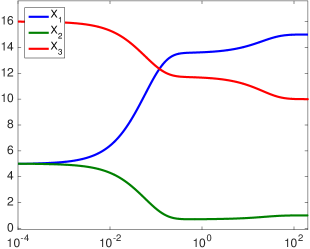
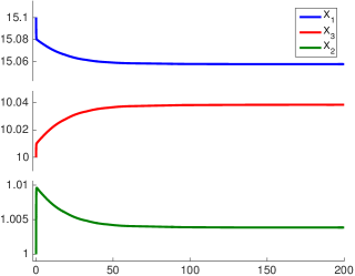
Example 2.1 (continued). First we demonstrate an adaptation experiment for a small but finite . Fix in (2). We perturb the system by adding of to the system. The evolution is shown in Figure 3. Next, in the limit of small perturbations, the matrix in (7) is found to be
The expressions (8) for Precision and Sensitivity imply that the we can obtain these two quantities by plotting the time trajectory of the corresponding entry in the matrix exponential . In this example we take to be the input and we plot the three entries in the first column of in Figure 4.
time [t] at 245 2
\pinlabel
conc.
[r] at -7 90
\pinlabel
conc.
[r] at -7 220
\pinlabel
conc.
[r] at -7 340
\endlabellist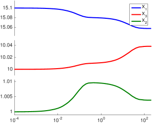 \labellist\pinlabeltime [t] at 265 0
\endlabellist
time [t] at 245 2
\pinlabel
concentration
[r] at -5 180
\pinlabel [b] at 273 345
\pinlabel [l] at 468 168
\endlabellist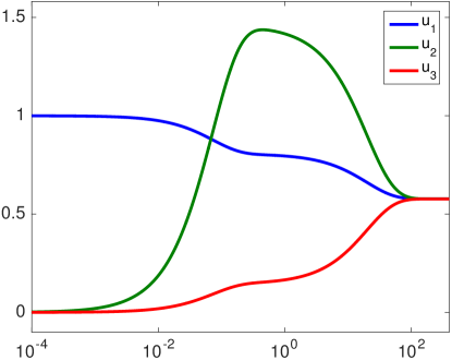
In the graph above one can read off the Sensitivity and Precision: choosing as output, the Sensitivity is the maximal value of over all time (about ), and the Precision is the limiting value of as time tends to infinity (). Note that the choice of input variable is encoded in the initial data for , and the choice of output variable means that we measure .
2.4. Maximization over parameters
As we mentioned in the introduction, in much of this paper we take the position that the stoichiometry of a system is given, and we ask within which bounds we can make Sensitivity and Precision vary by the freedom of choosing coefficients and . This leads to the following three numbers:
The maximal inverse Precision plays a role in characterizing maximal Sensitivity (see Section 4.3).
Example 2.4 (Arbitrarily large and ). We generalize Example A by replacing with for some and a choice of for input and for output.
We want to explore the values of Precision and Sensitivity. Since the system is small we are able to explicitly calculate the Precision directly from Definition 2.8 as follows. The stoichiometric matrix enforces that is constant along time trajectory of concentrations in every stoichiometric simplex. Therefore , where is a positive constant. Let be the perturbed steady state when is added to and then . For both steady states we have . With these relations the calculation of inverse Precision is straightforward:
| (10) |
We observe that by choosing the ratio large enough, one can have arbitrarily high Precision, i.e. .
This example is able to show Sensitivity arbitrarily close to , i.e. . It is an easy exercise to show that the first reaction, as a subsystem, has , and consequently . If we choose in such a way that the first reaction happens much faster than the second, then can rise arbitrarily close to and after some time that the second reaction takes place, it comes down arbitrarily close to 0. Figure 5 shows the plot of for three values of .
time [t] at 207 2
\pinlabel
concentration
[r] at -2 180
\endlabellist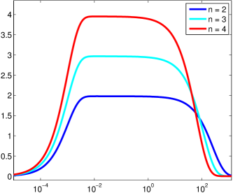
3. Results: Properties of the Precision
As described above, the aim of this paper is to explore the degree to which detailed-balance, mass-action systems can have large Sensitivity and large Precision. In this section we focus on the Precision, and prove two main results. The first is an explicit formula for homogeneous systems; the second is a characterization of the minimal Precision in terms of the stoichiometry, which will be of use in Section 4.
We choose a system , and we fix an input species and an output species .
In some cases the Precision can be calculated explicitly. Example 2.4 above is an instance of this; another instance is the class of homogeneous systems. A reaction network is called homogeneous of order if for fixed, all the reactions are of the type
Each column of in such reaction network consists of two nonzero elements with values and . Therefore , which implies that is constant in each stoichiometric simplex. Below we derive an explicit formula for the Precision of homogeneous systems.
Theorem 3.1 (Precision for homogeneous systems).
If a reaction network is homogeneous of some order , then for any input and output
| (11) |
Example 3. Unimolecular reactions are a good example of a homogeneous reaction network. Below we present a reaction diagram between four species. Letting be the input, the inverse Precision for the three other species is (see (11)).
\labellist\pinlabeltime [t] at 255 15
\pinlabel
concentration
[r] at -2 130
\endlabellist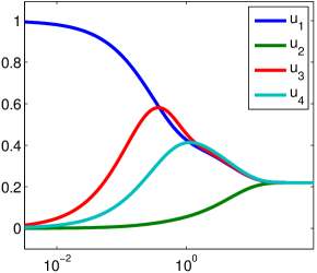 \schemestart\arrow(x1–x2)¡=¿[][45] \arrow(–x3)¡=¿[][-45]
\arrow(@x1–x4)¡=¿[][][-45] \arrow(–)¡=¿[][][45]
\arrow(@x1–@x3) ¡=¿[]
\schemestop
Proof.
Fix the parameters . Equation (3) implies that at any steady state , for a reaction involving species and , the ratio equals and thus is the same for each steady state. This implies that all steady states are multiples of each other. On the other hand we have a conservation law for some positive constant . In view of the definition of Precision (following the notation of Section 2.3) we have . This can be written as
in which the denominator is a sum of constant steady state ratios, hence independent of . Finally the inverse Precision is
∎
Note that the Precision for such a homogeneous network is always larger than one, and can be made arbitrarily large by tuning —specifically, by making the stationary concentration of the input variable small with respect to the other concentrations. This might seem like a good thing; however, we will see below that such a choice makes it difficult to have high Sensitivity, and therefore ‘good’ systems do not choose this route.
In fact, as we shall see in Section 4, there is a strong suggestion that having high Sensitivity requires low Precision for a subsystem. Because of this reason, it is interesting to consider lower bounds on Precision, or equivalently, upper bounds on inverse Precision. In the rest of this section we characterize the maximal inverse Precision for a given system ,
in terms of the stoichiometry of the system, ie. in terms of .
The support of a vector is . Considering a linear space , we say that a vector is elementary if is nonzero and is minimal in , i.e. there exists no nonzero with . The orthogonal complement of is
In the following theorem, maximal inverse precision is characterized in terms of elementary vectors of and , where . Observe that if and , then and hence ; so each describes an invariant linear combination of the stoichiometric simplex .
Theorem 3.2 (Sharp upper bounds on inverse Precision).
Fix a system and input and output species , and let . Then:
| (12a) | ||||
| (12b) | ||||
| (12c) | ||||
Recall Example A, where we already observed that , and . Therefore all elementary vectors in are multiples of , and the characterization (12b) reduces to the maximum over two elements:
For (12c), the space has three elementary vectors, up to scalar multiples, which are , , and . Recall that the input variable is 1, and the output variable 2; therefore of these three directions, the third does not appear in the maximum, since it can not be rescaled to have . The maxmimum in (12c) then reduces to
Example 3. As an example where the alternative options and are relevant, consider the single reaction
Here , , and ; therefore has only the elementary vector , up to scalar multiplication, and (12c) reduces to
In this case has elementary vectors , , and , so that (12b) becomes
Indeed, the reaction has negative Precision for all positive values of (since increase in always leads to decrease in .) Therefore the max inverse Precision can reach zero, but can not be positive.
The maxima (12b) and (12c) may be evaluated by enumerating the elementary vectors of a linear space. We will describe an algorithm for this in Section 5.
The rest of this section is devoted to the proof of this theorem, through a series of lemmas. The first lemma provides the connection between inverse Precision on one hand and the vectors and that appear in Theorem 3.2.
Lemma 3.3.
For given , the conditions
| (13) |
uniquely determine the pair . Then
| (14) |
As a consequence,
Proof.
The existence of a satisfying (13) will follow from the argument in the next paragraph; here we show that satisfying (13) is unique. If not, then there are distinct satisfying (13). Then is a nonzero vector such that and , so that , and consequently . Since has strictly positive components, this implies , a contradiction.
We now show (14). For each , write for the unique stationary state in the same stoichiometric simplex as . By Lemma 2.4, is a smooth function of ; we write , which is the vectorial rate of change of the stationary state as we add component . Again by Lemma 2.4, , and by differentiating we find . From follows , and therefore we find that satisfies the two equations
Defining these can be rewritten as
which is equivalent to (13). This also proves the existence of a solution to (13). The fact that (equation (14)) is then a direct consequence of (9). ∎
Remark 3.4 (Chemical interpretation of and ).
The proof of this lemma illustrates the chemical interpretation of and . Both are defined in terms of a curve of stationary states generated by perturbing the system by adding small amounts of :
-
(1)
can be interpreted as the derivative of the vector function at , i.e. times the rate of change of the vector of chemical potentials of the species;
-
(2)
can be interpreted as the (infinitesimal) stoichiometrically admissible perturbation that connects the non-stationary point with the stationary point : .
∎
In the following lemmas we characterize the maximal inverse precision, where the maximum is taken over all , in terms of elementary vectors in and . Lemmas 3.5, 3.7, and 3.8 together conclude the proof of Theorem 3.2.
Lemma 3.5.
Proof.
The condition
| (15) |
implies for that if , then ; if , then ; and if , then . Moreover, if , then
a contradiction. Hence . Summarizing, we find that (15) implies
| (16) |
So for fixed , if , then and the result is trivial. Otherwise the supremum
| (17) |
is bounded from above by
| (18) |
This is a linear optimization problem. To complete the proof of this lemma, we will argue that for each fixed , (18), and hence (17), is bounded from above by
If the supremum in (18) equals , then there exist and such that satisfies (16) for all , with and . But then , contradicting that . So the value of (18) is finite, and hence the optimum is attained. Let be an optimal solution such that is as small as possible.
We show that or is an elementary vector. If not, then and there is a nonzero vector so that , by the definition of an elementary vector. We may assume that ; otherwise replace with . Then
is attained by an optimal solution which satisfies one of the inequalities in (16) with equality, such that where for some . Since and , that would contradict the choice of as an optimal solution of (18) with minimal support.
So is elementary, and it remains to show that . If , we have , and hence . Hence . If , then for a sufficiently small , the vector is a feasible solution of (18) with , contradicting the optimality of . Hence , as required. ∎
We need the following, essentially combinatorial fact on elementary vectors. For any and , let denote the submatrix of spanned by the rows and columns in resp. .
Lemma 3.6.
Let be elementary in . Then there exist a set , elementary vectors for , and elementary vectors for , such that
-
•
, and ;
-
•
for each , and ; and
-
•
for each , and .
Proof.
Consider the set . The rows of are independent, for if there were a linear dependency among these rows, then there would exist a nonzero vector with , contradicting our assumption that is elementary vector of .
Pick any maximal set so that and so that the rows of are still independent. Then the rows of form a basis of the rowspace of . Let be such that the columns of are a basis of . Then by applying column operations to (as in standard Gaussian elimination) we may obtain a matrix of the form
That is, , and as column operations do not change the column space, . For each , let denote the unique column of with a 1 in the -th row. Then and by construction, and moreover is elementary: any is a linear combination of the columns of , so that if , then must be a scalar multiple of .
To obtain the vectors , we construct the matrix as
using the matrix . Since and , the columns of span . For each , let denote the unique column of with a 1 in the -th row. Then , , and is elementary as before. ∎
We comment on the relation with matroid theory in Section 5.
Lemma 3.7.
Proof.
First, note that the supremum is necessarily nonnegative, since if is feasible in combination with some , then so is for any . So it remains to show that if is an elementary vector with , then the supremum is at least . As we have already established that the supremum is nonnegative, we may assume .
To prove that the supremum is at least , it suffices to show that for any , there are such that and
This condition is equivalent to
| (19) |
We will construct such vectors , using a set and vectors and as in Lemma 3.6. Throughout, we will preserve that
| (20) | ||||
| (21) | ||||
| (22) |
In each step, we increase the cardinality of , until we attain . Then, we necessarily have (19).
We initialise by setting
| (23) |
To see that (20) holds for this initial , note that , so that we need only verify that . Since , we have , as required. As , condition (21) is vacuously satisfied by . It remains to show (22), that . We have , , and hence ; moreover , , and , so that . So , and as , we have . Hence , as required.
In the general step, if there is an , we put
where is chosen such that and with sufficiently small to ensure that for each with , the sign of is unaltered. Then after this step, we have , and (20), (21), and (22) are preserved. If there is an , we similarly put
with and sufficiently small.
Since each may be chosen arbitrarily close to , we can ensure that in the final stage
∎
Lemma 3.8.
Proof.
We first prove ‘’. Let attain the maximum on the left. By Lemma 3.6, there is a set and vectors so that , and , and for each , and . Pick . Then , and . As , we have
As is elementary, is a feasible solution of the maximum on the right. Hence ‘’. Interchanging with , and with , we obtain the converse inequality ‘’. ∎
This completes the proof of Theorem 3.2.
Example 3. We illustrate the proof by considering a system with 6 species and reactions
The stoichiometric space and its orthogonal complement contain the following elementary vectors:
These lists are complete, that is, each elementary vector of (resp. ) is obtained by scaling one of the vectors (resp. ). With input and output , inspection of both tables reveals that the maxima
| (24) |
are attained by the elementary vectors and , respectively.
Using the algorithm of Lemma 3.7, we construct vectors , , which are feasible in
and such that is arbitrarily close to the maximum .
The vector has , and we use in the algorithm. In the initial step, we put , where . Then , , and we have , and . To repair that and , we use the elementary vector with . We have , so we put where . Then, we consider that and , and add a small multiple of to compensate: with . Next, we have and , and so we add a small multiple of where . Finally, we repair that whereas , and put with .
We end up with
where . Constructing by setting for and , we obtain the feasible triple as follows:
Here we abbreviated , and the approximation of is based on the assumed relative magnitudes of the . The objective value of tends to the maximum 3 as , and at the same time .
One way the construction of above can be interpreted is as follows. The optimum in (24) is achieved in and . Focusing on the -side of this characterization, first note that each of the elementary vectors is uniquely characterized by its support, up to multiplication by scalars, by the very definition of an elementary vector. Therefore the optimal vector is characterized by its zeros for coordinates and . One can now force the system to follow by choosing such that and are much smaller than the other coordinates. Although in a relative sense and participate in the reactions—as illustrated by the values in the table above, which give and —because of the low background concentrations they play no role in terms of absolute concentrations (as illustrated by the low values of ). The end result is that the system becomes similar to a single equation with stoichiometry , with small perturbations of other reactions. The construction above makes this statement concrete.
4. Results: Properties of the Sensitivity
We now turn to the Sensitivity. In contrast to the Precision, the Sensitivity is a dynamic property, that depends not only on the stationary state but also on the dynamic rates . Our aim is, as before for the Precision, to find estimates from above and below on the Sensitivity that depend on the stoichiometry but not on the parameters and .
4.1. Upper bounds
Our first result gives a very general upper bound on Sensitivity for all mass-action, detailed-balance systems.
Theorem 4.1 (General upper bound on Sensitivity).
Given a kinetic system , we have the Sensitivity bound
Proof.
Let be the solution of (7) with initial datum . Set . Then solves the equation
| (25) |
Since is symmetric and non-positive, it can be diagonalized with orthogonal matrices, , where is a diagonal matrix of non-positive eigenvalues, and . Then , and we calculate, writing for the -th column vector of ,
Since the eigenvalues are non-positive, this latter expression is bounded in absolute value by
We will see in the examples below (e.g. Example 4.3) that this bound is very far from being sharp.
Remark 4.2 (Upper bound for normal systems).
If in (7) is normal, it is orthogonally diagonalizable. Therefore by the same argument for in the previous theorem we have . ∎
Following the explicit formula for the Precision of homogeneous systems, one can also prove a property of the Sensitivity of homogeneous systems:
Theorem 4.3 (Upper bound on Sensitivity for homogeneous systems).
If the system is homogeneous of some order , then .
Proof.
We begin by introducing
and we can assume without loss of generality that each reacting pair is only connected by one reaction. Each column of has only two nonzero entries, which implies that the intersection of supports of two different rows of has at most one element. Thus the matrix in (7) reads
The matrix has negative diagonal and nonnegative off-diagonal entries. Based on this observation we proceed with the proof. Let be the identity matrix, then for all there exists such that is element-wise nonnegative. We denote this property by . Powers of such a matrix preserve the property. The matrix exponential is an infinite sum of elementwise nonnegative matrices, hence . On the other hand the two matrices and commute. By the properties of matrix exponentials we obtain
The matrix has the property that the sum of the entries of each row is zero. Let , then which implies that . Each row sum of nonnegative entries of is 1, therefore for all . The alternative formulation of Sensitivity (8) then completes the proof:
∎
The value is special, for the following reason. In some cases one can concatenate, or ‘daisy-chain’ systems, by feeding the output of one system into the input of another. We conjecture that the sensitivity of the chain can never exceed the product of the sensitivities of the individual components. If this is true, then the value is critical; it only makes sense to daisy-chain components with . Whether the conjecture is true or not, for some systems tuning of the parameters allows one to approximately achieve product Sensitivity, as the next example shows.
Example 4.1 (Daisy chaining) We extend Example A to the following set of reactions:
The parameters and are chosen to give rise to four separate timescales, as shown in Figure 7. A perturbation in input in the first reaction, which is the fastest, results in a quick rise in . In the second reaction the species behaves like an input and amplifies . Species shows a Sensitivity near 2 relative to , and near relative to . This chaining is further extended by feeding to , obtaining a Sensitivity close to for relative to input . The final reaction is the slowest one, and acts as a buffer whose concentration is considerably larger than the other species. At the slowest time scale, the last reaction reduces the initial rise in and pushes back all the species to a concentration very close to pre-stimulus level, thus creating a large Precision.
time [t] at 245 2
\pinlabel
concentration
[r] at -8 200
\endlabellist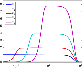
4.2. Intermezzo: subsystems
In Theorem 4.5 below we construct lower bounds for the maximal Sensitivity by using properties of a subsystem and exploiting the possibility of making the subsystem dynamics much faster than the dynamics in the remainder of the system. We first study the relation between optimal Precision and Sensitivity of a subsystem with that of the full system.
Definition 4.4 (Subsystems).
is a subsystem of , notation , if and is the restriction of to the columns given by .
One can obtain a subsystem by setting the rates of some of the reactions to zero. Note that this is different from setting them to nearly zero, since the stoichiometric freedom is different in the two cases, and therefore the stationary states are also different.
Theorem 4.5 (Precision and Sensitivity under taking subsystems).
If is a subsystem of , then
-
•
The maximal Sensitivity of the subsystem is less than or equal to the maximal Sensitivity of the full system, and
-
•
The maximal and minimal Precision of the subsystem may be smaller than, equal to, or larger than in the full system.
Proof.
For the purposes of Precision and Sensitivity, the two systems (the ‘system’ and the ‘subsystem’) are both described by equations of the form (7). We can take the same set of reactions for both, if for the duration of this proof we allow some of the parameters for the subsystem to be zero.
The behaviour of the Sensitivity now follows from the continuity properties of ordinary differential equations. We write the solution of (7) with initial datum as to emphasize the choice of parameters. For each , we can find a parameter point for the subsystem (which implies that some of the are zero), and a time , such that
On the finite time interval , solutions depend continuously on parameters, implying that we can find strictly positive parameter points for the full system such that
Since is arbitrary, it follows that
A similar argument fails for the Precision, since the two limits and need not commute. As examples where the Precision of a system is larger or smaller than the Precision of a subsystem, consider
-
•
If we choose a system with finite Precision and a subsystem in which the input and output species are no longer connected by any reactions, then the output concentration is independent of the input concentration, implying an infinite Precision, which is therefore larger than the Precision of the full system.
-
•
In Example 4.1 the Precision of the full system is high, while some of the subsystems have low Precision.
∎
4.3. Properties of the Sensitivity: lower bounds
Since , the inequality always holds (compare the definitions of Sensitivity (5) and Precision (6)) and therefore . The next theorem strengthens this property.
Theorem 4.6 (Maximal Sensitivity is bounded from below by the maximal inverse Precision over all subsystems).
Given a system ,
Proof.
The proof of this theorem is very similar to that of Theorem 4.5. For any and , we choose a parameter point for (i.e. with whenever ) such that
We then choose such that
Finally, using continuous dependence on parameters we choose a strictly positive parameter point such that
Therefore
and since and the subsystem were arbitrary, the result follows. ∎
Example 4.3 (Sensitivity larger than maxInvP). We consider a chemical reaction network with 6 species and three reactions:
Choosing to be the input and the output, Theorem 3.2 gives . Figure 8, however, shows a value for the sensitivity of about , which therefore exceeds . A formal argument inspired by a numerical observation suggests that the Sensitivity is bounded from above by , but proving this bound remains open.
time [t] at 255 2
\pinlabel
concentration
[r] at -7 190
\endlabellist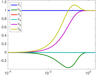
5. Matroid theory and the proof of Theorem 3.2
5.1. Matroids and the combinatorics of the stoichiometric space
The proof of Theorem 3.2 was conceived with a certain matroid related to the stoichiometric matrix in mind. Seeing that the entire argument could be also stated in terms of linear algebra, we chose to avoid the use of this concept in our presentation of the proof. We will give the matroid perspective here as an optional service to the reader. We briefly describe the relevant matroid theory here, referring to the book of Oxley [Oxl14] for a more detailed account and full proofs of the statements below.
Consider a finite set of vectors and let
Then has the following three properties.
-
(I0)
-
(I1)
if and , then
-
(I2)
if and , then there exists an so that .
A matroid is any pair where is a finite set and is a set of subsets of satisfying the above three axioms. In this more abstract setting, we also call a set independent if and dependent otherwise. A set is called a basis if is an inclusion-wise maximal independent set, and is a circuit if is an inclusion-wise minimal dependent set.
Let be a matroid, and let be the set of bases of . Then the set
is the set of bases of another matroid , the dual of .
Given this elementary result in matroid theory, the proof of the following statement is straightforward.
Lemma 5.1.
If is a circuit of and , then there is a basis of such that
-
•
, and ;
-
•
for each , there is a circuit of such that ; and
-
•
for each , there is a circuit of such that .
Proof.
As is a circuit of , the set is an independent set. Let be any inclusion-wise maximal set containing . Then is a basis of . Since is independent, the circuit cannot be fully contained in , so . Since is maximal, the set is dependent for each , and hence contains a circuit of . By definition of the dual, is a basis of . Since is a maximal independent set of , the set is dependent in for each , hence contains a circuit of . ∎
Given any matrix , define
Then is a linear matroid.
Lemma 5.2.
Let be an matrix, and let . Then is a circuit of if and only if for an elementary vector .
Proof.
A set is dependent in if and only if there is a linear dependency among the columns of pointed out by , i.e. a nonzero vector with and . ∎
The circuits of the dual of can be similarly characterized.
Lemma 5.3.
Let be an matrix, and let . Then is a circuit of if and only if for an elementary vector .
Now the stoichiometric matrix is an matrix, and thus the transpose matrix is an matrix. The matroid has ground set and divides the subsets of in dependent and independent sets. With , the circuits of are the minimal supports of vectors , and the circuits of are the minimal supports of vectors .
5.2. Computing the upper bound on the inverse precision
Let be a circuit of the stoichiometric matroid . Finding a vector with and is a matter of elementary linear algebra. Computing the maximum
reduces to enumerating the collection of circuits of the stoichiometric matroid. In the same vein, to determine
it suffices to enumerate the circuits of .
The number of circuits of a matroid on elements can be exponential in , and so we cannot expect to enumerate the full set of circuits in polynomial time. Boros et al. [BEGK03] describe a simple algorithm which will enumerate the circuits of a matroid in incremental polynomial time. That is, there exists a polynomial so that listing the first circuits of a matroid takes their algorithm time. In a related paper [KBE+05], an algorithm is described which will generate the circuits containing a fixed element in incremental polynomial time. For our application, we would like to enumerate the circuits containing two fixed elements of the ground set, but it appears to be an open problem whether this can be done in incremental polynomial time. On the practical side, SAGE, the open-source computer algebra system, implements several algorithms for enumerating the circuits of a matroid.
Given that there are two ways to determine the upper bound, whose running times will depend on the number of circuits of or , one would like to estimate which one of these matroids has the least number of circuits.
It is straightforward that in in a matroid, any two bases have the same cardinality. The rank of a matroid is the cardinality of any basis of . A matroid of rank on elements may have as many as circuits, the maximum being attained by the uniform matroid of rank .
The rank of the stoichiometric matrix equals , and the rank of its dual is , where is the size of the ground set. Taking the maximum number of circuits of a matroid of rank as a coarse estimate for the true number of circuits, we expect that in general will have fewer circuits than while .
6. Non-detailed-balance chemical reaction networks
We now briefly comment on systems with mass-action kinetics but without the detailed-balance assumption. In these systems the kinetic function has the form
| (26) |
where and are as in Definition 2.1, and and are arbitrary non-negative coefficients. The network is called reversible if .
In the case of detailed-balance systems, we chose to perturb the system by adding a small amount of a certain species. Although in non-detailed-balance systems there are more choices for perturbation, here we stick to the same method. Definitions 2.7 and 2.8 for Sensitivity and Precision do not rely on the assumption of detailed balance, whereas in the alternative formulations (8), the matrix appears and this matrix owes its structure to the detailed-balance assumption. First we provide an alternative formulation for non-detailed-balance systems.
Lemma 6.1 (Alternative formulations of Precision and Sensitivity in non-detailed-balance systems).
Let be the solution of with
and initial data . The Precision and Sensitivity then have the alternative formulations
| (27) |
Proof.
The proof is again a simple manipulation. ∎
One can ask what happens with the bounds on Precision and Sensitivity when detailed balance does not hold. We start by obtaining a bound for reversible unimolecular reaction networks that do not necessarily satisfy detailed balance.
Theorem 6.2.
In a reversible unimolecular reaction network we have .
Proof.
Reactions in such a network are of the type
with both rate constants and strictly positive when and react with each other and we assume them to be zero otherwise. This allows to write the following ODE for the evolution of each species.
Let , then solves where
We note that has negative diagonal and nonnegative off-diagonal elements, moreover . Showing that is similar to the argument in Theorem 4.3. ∎
Consider the following example of how a small system can achieve large Sensitivity and Precision.
Example 6 (Adaptation in non-detailed-balanced systems). Consider a receptor , a ligand , a phosphate group , complexes , , , and (all indexed from 1 to 7 respectively) that participate in reactions depicted in Figure 9. Let serve as input and output of the network. Figure 9 shows how in the absence of detailed balance a Sensitivity near 70 can be achieved. Note that the detailed-balance version of the network has . In fact, if we omit the last reaction, then with the same parameters an inverse Precision near 70 is achieved. The last reaction acts as a feedback with delay and performs the adaptation step. One can further increase the Precision by increasing the concentration of and making sure that the last reaction is the slowest one.
time [t] at 245 2
\pinlabel
concentration
[r] at -5 180
\endlabellist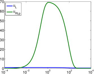

7. Summary and Discussion
7.1. Summary
The analysis of this paper is sparked by the question we posed in the Introduction, To which extent can a non-dissipative system perform adaptation? We investigated this question by first defining ‘non-dissipative’ as ‘detailed-balance, mass-action’ and ‘performing adaptation’ as ‘having high Sensitivity and Precision’, and then deriving a number of rigorous results about such systems.
Concretely, we prove that
- (1)
-
(2)
The maximal inverse Precision of a given system can be characterized in various combinatorial ways (Theorem 3.2);
- (3)
- (4)
In this way we show that non-dissipative systems can be arbitrarily adaptive. This does require ‘extreme’ systems however, in the sense of having large stoichiometry, large concentration ratios, and/or large time scale ratios. Theorem 4.1 shows that large concentration ratios are necessary for large Sensitivity. For the other two we have no rigorous characterization, but the examples suggest that at least large stoichiometry (Example 2.4) or large time scale ratios (Example 4.1) are necessary for good performance.
7.2. Discussion
We now comment on a number of aspects of this work.
Definition of ‘non-dissipative’ systems. Detailed-balance, mass-action systems are a natural choice for ‘non-dissipative’ systems. They can be considered thermodynamically closed, and admit a free-energy functional that drives the evolution in a gradient-flow structure [GM13, MM]. In this context, one can identify ‘dissipation’ with the instantaneous decrease of , and the system is therefore non-dissipative in the sense that at all stationary points is constant.
Despite these nice properties, this family does contain some weird specimens, such as
for which the stoichiometric subspace is the whole space of positive concentrations, and which clearly can not be mass-conservative in the traditional sense. In our examples we avoided such exotic species, and concentrated on systems that can be realized with actual chemical systems.
Relation between ‘adaptation’ and Precision and Sensitivity. In this paper we focus on Precision and Sensitivity as proxies for a more elaborate concept of adaptation. A better concept of adaptation might include (a) the persistence of ‘good’ behaviour across a range of input concentrations, allowing for continuous tracking in the direction of increasing concentration, and (b) a measure of ‘temporary response’ that measures not the instantaneous maximum of a concentration (like our Sensitivity) but some quality of a downstream machinery that acts on this concentration.
Role of matroid theory. The proof of the characterization of maximal inverse Precision, Theorem 3.2, is formulated in linear-algebra terminology, but in fact the ideas are inspired by matroid theory, as explained in Section 5. Matroid theory arises in this context through the maximization over positive coefficients and , by which equality constraints become replaced by sign constraints (Lemma 3.5 is a good illustration of this). The framework of matroid theory provides a natural structure in which to connect different characterizations of the same object, as illustrated by Theorem 3.2, and for this reason has been used in other works on chemical reaction networks [BBCQ04, MRS14, Rei14].
Role of definitions. The conclusion of this paper, that non-dissipative systems can perform arbitrarily effective adaptation, serves as an illustration that the relationship between dissipation and functionality that is often broadly claimed in the literature requires very careful consideration; precise definitions are necessary, and at this stage it is not quite clear how to best choose these definitions, in order to obtain the clearest statements and most useful insight.
7.3. Comparison with [LSN+12, LT13]
The results of this paper appear to be in contradiction with remarks by Lan, Tu, and co-authors [LSN+12, LT13] that e.g. ‘adaptation is necessarily a non-equilibrium process and it always costs (dissipates) energy’ [LSN+12] or ‘the I1-FFL (Incoherent type-1 feed-forward loop) network always operates out of equilibrium’ [LT13].
The discrepancy stems from a difference in definitions: both papers assume a type of feedback that only exists in non-equilibrium systems. Consider, as an example, the simple reaction . From one point of view, this reaction encodes only positive influence of on and vice versa, since starting from equilibrium, increasing leads to increase in . From this point of view, a negative feedback mechanism can not be built using equilibrium building blocks, since negative feedback would require a negative influence. The systems of the present paper therefore fall outside of the scope of [LSN+12, LT13].
However, in this simple reaction one can also observe negative influence, through the mechanism of redistribution. Consider for instance the following quantitative version:
(This corresponds to , , and in the setup of this paper). If, starting from equilibrium , , we increase both and by the same amount, then the reaction will redistribute the total additional amount in the ratio , as illustrated in Figure 10. This has the same qualitative effect as negative feedback of on would have, as illustrated by the figure.
time [t] at 245 2
\pinlabel
concentration
[r] at -7 90
\pinlabel
concentration
[r] at -7 300
\endlabellist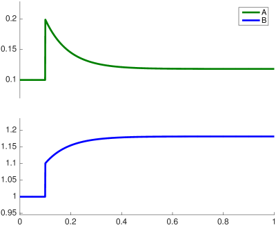
This simple example allows us to explain how the non-dissipative systems of this paper have an effect very similar to the incoherent type-1 feed-forward loop (I1-FFL) studied in [LT13]. Consider the following two systems:
\arrow(x1–x3)-¿[-90,2] \arrow(@x1–x2)-¿[-50,1.2] \arrow(–x3)-—[-130,1.2] \schemestop
\arrow(x1–x3)s¿[+(-70:1.3)][-90,2] \arrow(@x1–x2)s¡¿[+(-70:1.3)][-50,1.2] \arrow(–x3)¡-¿[][][-130,1.2] \schemestop
The system on the left is such an incoherent feed-forward loop, depicted using the traditional biochemical notation for positive and negative influence, while the system on the right is that of Example A of this paper, reformatted to resemble the system on the left. The basis for the adaptive effect of the I1-FFL is the difference in time scale between the fast activation , which first leads to increase of , and the slow inhibition , which reduces again on a longer time scale.
We can recognize the same working principle in the system of Example A on the right. An increase in input leads to an increase in both and ‘output’ ; on the slower time scale of reaction , the redistribution effect just described then reduces the value of .
To conclude, the apparent discrepancy between the results of Lan, Tu, and co-authors on one hand and those of this paper can be traced back to a focus on different systems; the systems of this paper lie outside of the scope of [LSN+12, LT13]. If the systems of this paper are taken into account, then it is clear that ‘good adaptive performance’, in the sense of high Precision and Sensitivity, can be achieved perfectly well in non-dissipative systems.
References
- [BBCQ04] D. A. Beard, E. Babson, E. Curtis, and H. Qian. Thermodynamic constraints for biochemical networks. Journal of theoretical biology, 228(3):327–333, 2004.
- [BDGC15] S. Bo, M. Del Giudice, and A. Celani. Thermodynamic limits to information harvesting by sensory systems. Journal of Statistical Mechanics: Theory and Experiment, 2015(1):P01014, 2015.
- [BEGK03] E. Boros, K. Elbassioni, V. Gurvich, and L. Khachiyan. Algorithms for enumerating circuits in matroids. In Algorithms and computation, volume 2906 of Lecture Notes in Comput. Sci., pages 485–494. Springer, Berlin, 2003.
- [BS13] J. P. Barton and E. D. Sontag. The energy costs of insulators in biochemical networks. Biophysical journal, 104(6):1380–1390, 2013.
- [CWOT15] Y. Cao, H. Wang, Q. Ouyang, and Y. Tu. The free-energy cost of accurate biochemical oscillations. Nature Physics, 2015.
- [ÉT89] P. Érdi and J. Tóth. Mathematical Models of Chemical Reactions: Theory and Applications of Deterministic and Stochastic Models. Manchester University Press, 1989.
- [Fel97] D. A. Fell. Understanding the Control of Metabolism. Portland Press, London, 1997.
- [GM13] A. Glitzky and A. Mielke. A gradient structure for systems coupling reaction–diffusion effects in bulk and interfaces. Zeitschrift für angewandte Mathematik und Physik, 64(1):29–52, 2013.
- [GSKA09] L. Goentoro, O. Shoval, M. W. Kirschner, and U. Alon. The incoherent feedforward loop can provide fold-change detection in gene regulation. Molecular cell, 36(5):894–899, 2009.
- [GtW13] C. C. Govern and P. R. ten Wolde. How biochemical resources determine fundamental limits in cellular sensing. arXiv preprint arXiv:1308.1449, 2013.
- [HJ72] F. Horn and R. Jackson. General mass action kinetics. Archive for rational mechanics and analysis, 47(2):81–116, 1972.
- [HS96] R. Heinrich and S. Schuster. The Regulation of Cellular Systems. Chapman & Hall, New York, 1996.
- [KBE+05] L. Khachiyan, E. Boros, K. Elbassioni, V. Gurvich, and K. Makino. On the complexity of some enumeration problems for matroids. SIAM J. Discrete Math., 19(4):966–984, 2005.
- [Lan61] R. Landauer. Irreversibility and heat generation in the computing process. IBM journal of research and development, 5(3):183–191, 1961.
- [Lan15] G. Lan. Energy dissipation drives the gradient signal amplification through an incoherent type-1 feed-forward loop. Physical Review E, 92(3):032702, 2015.
- [LHW08] S. Lapidus, B. Han, and J. Wang. Intrinsic noise, dissipation cost, and robustness of cellular networks: The underlying energy landscape of MAPK signal transduction. Proceedings of the National Academy of Sciences, 105(16):6039–6044, 2008.
- [LSN+12] G. Lan, P. Sartori, S. Neumann, V. Sourjik, and Y. Tu. The energy-speed-accuracy trade-off in sensory adaptation. Nature physics, 8(5):422–428, 2012.
- [LT13] G. Lan and Y. Tu. The cost of sensitive response and accurate adaptation in networks with an incoherent type-1 feed-forward loop. Journal of The Royal Society Interface, 10(87):20130489, 2013.
- [MHL12] A. Murugan, D. A. Huse, and S. Leibler. Speed, dissipation, and error in kinetic proofreading. Proceedings of the National Academy of Sciences, 109(30):12034–12039, 2012.
- [MM] J. Maas and A. Mielke. On gradient structures for chemical reactions with detailed balance: I. Modeling and large-volume limit.
- [MRS14] S. Müller, G. Regensburger, and R. Steuer. Enzyme allocation problems in kinetic metabolic networks: Optimal solutions are elementary flux modes. Journal of theoretical biology, 347:182–190, 2014.
- [MS12] P. Mehta and D. J. Schwab. Energetic costs of cellular computation. Proceedings of the National Academy of Sciences, 109(44):17978–17982, 2012.
- [MTES+09] W. Ma, A. Trusina, H. El-Samad, W. A. Lim, and C. Tang. Defining network topologies that can achieve biochemical adaptation. Cell, 138(4):760–773, 2009.
- [Oxl14] J. Oxley. What is a matroid? http://www.math.lsu.edu/~oxley/survey4.pdf, 2014.
- [QR05] H. Qian and T. C. Reluga. Nonequilibrium thermodynamics and nonlinear kinetics in a cellular signaling switch. Physical review letters, 94(2):028101, 2005.
- [Rei14] A. C. Reimers. Metabolic Networks, Thermodynamic Constraints, and Matroid Theory. PhD thesis, Freie Universität Berlin, 2014.
- [SGLH14] P. Sartori, L. Granger, C. F. Lee, and J. M. Horowitz. Thermodynamic costs of information processing in sensory adaptation. PLoS computational biology, 10(12):e1003974, 2014.
- [SNMW13] M. Skoge, S. Naqvi, Y. Meir, and N. S. Wingreen. Chemical sensing by nonequilibrium cooperative receptors. Physical review letters, 110(24):248102, 2013.
- [SRA+08] A. Saltelli, M. Ratto, T. Andres, F. Campolongo, J. Cariboni, D. Gatelli, M. Saisana, and S. Tarantola. Global Sensitivity Analysis: The Primer. John Wiley & Sons, 2008.
- [Szi29] L. Szilard. Über die Entropieverminderung in einem thermodynamischen System bei Eingriffen intelligenter Wesen. Zeitschrift für Physik, 53(11-12):840–856, 1929.
- [Tu08] Y. Tu. The nonequilibrium mechanism for ultrasensitivity in a biological switch: Sensing by Maxwell’s demons. Proceedings of the National Academy of Sciences, 105(33):11737–11741, 2008.
- [WXW08] J. Wang, L. Xu, and E. Wang. Potential landscape and flux framework of nonequilibrium networks: Robustness, dissipation, and coherence of biochemical oscillations. Proceedings of the National Academy of Sciences, 105(34):12271–12276, 2008.
- [XZWW13] L. Xu, F. Zhang, E. Wang, and J. Wang. The potential and flux landscape, Lyapunov function and non-equilibrium thermodynamics for dynamic systems and networks with an application to signal-induced Ca2+ oscillation. Nonlinearity, 26(2):R69, 2013.