Hyperinflation in Brazil, Israel, and Nicaragua revisited

Abstract

The aim of this work is to address the description of hyperinflation regimes in economy. The spirals of hyperinflation developed in Brazil, Israel, and Nicaragua are revisited. This new analysis of data indicates that the episodes occurred in Brazil and Nicaragua can be understood within the frame of the model available in the literature, which is based on a nonlinear feedback (NLF) characterized by an exponent $\beta>0$. In the NLF model the accumulated consumer price index carries a finite time singularity of the type $1/(t_{c}-t)^{(1-\beta)/\beta}$ determining a critical time $t_{c}$ at which the economy would crash. It is shown that in the case of Brazil the entire episode cannot be described with a unique set of parameters because the time series was strongly affected by a change of policy. This fact gives support to the “so called” Lucas critique, who stated that model’s parameters usually change once policy changes. On the other hand, such a model is not able to provide any $t_{c}$ in the case of the weaker hyperinflation occurred in Israel. It is shown that in this case the fit of data yields $\beta\to 0$. This limit leads to the linear feedback formulation which does not predict any $t_{c}$. An extension for the NLF model is suggested.

There are $10^{11}$ stars in the galaxy. That used to be a huge number. But it’s only a hundred billion. It’s less than the national deficit! We used to call them astronomical numbers. Now we should call them economical numbers.

Richard Feynman

I Introduction

Inflation contribution is fundamental to reach the “economical numbers” quoted by Feynman (see data plotted below). But most importantly, when inflation surpasses moderate levels it affects real economic activities. Models of hyperinflation are especially suitable to emphasize that inflation implies bad “states of nature” in economy. Wars, states bankruptcies, and changes of social regimens are the characteristics of such regimens. These issues are analyzed in textbooks on econophysics stanley99 ; stauffer99 ; sornette03b .

The model for hyperinflation available in the literature is based on a nonlinear feedback (NLF) characterized by an exponent $\beta>0$ of a power law. In such an approach the accumulated consumer price index (CPI) exhibits a finite time singularity of the form $1/(t_{c}-t)^{(1-\beta)/\beta}$. This feature allows to determine a critical time $t_{c}$ at which the economy would crash. Although this model has been successfully applied to many cases sornette03 ; szybisz08 ; szybisz09 ; szybisz10 ; szybisz15 , the authors of Ref. sornette03 found difficulties in determining $t_{c}$ for regimes of hyperinflation occurred in Brazil, Israel, and Nicaragua. Therefore, the present work is devoted to revisit these episodes. It is shown that after a revision of data is possible to predict reasonable values of $t_{c}$ for Brazil and Nicaragua. However, in the case of Israel the difficulty persists, this feature would be plausibly attributed to permanent but partial efforts for stopping inflation. In order to follow better the evolution of inflation we provide brief historical descriptions for these countries.

The paper is organized in the following way. In Sec. II the NLF theory is outlined with details in order to present self-consistently the tools applied for analyzing regimes of hyperinflation. The episodes occurred in Brazil, Israel, and Nicaragua are revisited in Sec. III. Finally, Sec. IV is devoted to summarize conclusions.

II Theoretical background

Let us recall that the rate of inflation $i(t)$ is defined as

$$i(t)=\frac{P(t)-P(t-\Delta t)}{P(t-\Delta t)}=\frac{P(t)}{P(t-\Delta t)}-1\>,$$ (1)

where $P(t)$ is the accumulated CPI at time $t$ and $\Delta t$ is the period of the measurements. In the academic financial literature, the simplest and most robust way to account for inflation is to take logarithm. Hence, the continuous rate of change in prices is defined as

$$C(t)=\frac{\partial\ln{P(t)}}{\partial t}\>.$$ (2)

Usually the derivative of Eq. (2) is expressed in a discrete way as

$$C(t+\frac{\Delta t}{2}) = \frac{\left[\ln P(t+\Delta t)-\ln P(t)\right]}{\Delta t}$$ (3)

$$= \frac{1}{\Delta t}\,\ln\left[\frac{P(t+\Delta t)}{P(t)}\right]\>.$$

The growth rate index (GRI) over one period is defined as

$$r(t+\frac{\Delta t}{2}) \equiv C(t+\frac{\Delta t}{2})\,\Delta t=\ln\left[\frac{P(t+\Delta t)}{P(t)}\right]$$

$$= \ln[1+i(t+\Delta t)]=p(t+\Delta t)-p(t)\>,$$

where a widely utilized notation

$$p(t)=\ln P(t)\>,$$ (5)

was introduced. It is straightforward to show that the accumulated CPI is given by

$$P(t)=P(t_{0})\,\exp{\left[\frac{1}{\Delta t}\int^{t}_{t_{0}}r(t^{\prime})dt^{\prime}\right]}\;.$$ (6)

II.1 Cagan’s model of inflation

In his pioneering work, Cagan has proposed cagan56 a model of inflation based on the mechanism of “adaptive inflationary expectation” with positive feedback between realized growth of the market price $P(t)$ and the growth of people’s averaged expectation price $P^{*}(t)$. These two prices are thought to evolve due to a positive feedback mechanism: an upward change of market price $P(t)$ in a unit time $\Delta t$ induces a rise in the people’s expectation price $P^{*}(t)$, and such an anticipation pushes on the market price. Cagan’s assumptions may be cast into the following equations:

$$1+i(t+\Delta t)=\frac{P(t+\Delta t)}{P(t)}=\frac{P^{*}(t)}{P(t)}=\frac{P^{*}(t)}{P^{*}(t-\Delta t)}\>,$$ (7)

and

$$\frac{P^{*}(t+\Delta t)}{P^{*}(t)}=\frac{P(t)}{P(t-\Delta t)}=1+i(t)\>.$$ (8)

Actually $P^{*}(t)/P(t)$ indicates that the process induces a non exact proportional response of adaptation due to the fact that the expected inflation $P^{*}(t)$ expands the response to the price level $P(t)$ in order to forecast and meet the inflation of the next period. Now, one may introduce the expected GRI

$$r^{*}(t+\frac{\Delta t}{2})\equiv C^{*}(t+\frac{\Delta t}{2})\,\Delta t=\ln\left[\frac{P^{*}(t+\Delta t)}{P^{*}(t)}\right]\>.$$ (9)

So, expressions (7) and (8) are equivalent, respectively, to

$$r(t+\frac{\Delta t}{2})=r^{*}(t-\frac{\Delta t}{2})\>,$$ (10)

and

$$r^{*}(t+\frac{\Delta t}{2})=r(t-\frac{\Delta t}{2})\>.$$ (11)

These relations imply

$$r(t+\Delta t)=r(t-\Delta t)\>,$$ (12)

giving a constant finite GRI equal to its initial value $r(t)=r(t_{0})=r_{0}$. The accumulated CPI evaluated using Eq. (6) leads to an exponential law

$$P(t)=P_{0}\,\exp{\left[r_{0}\,\biggr{(}\frac{t-t_{0}}{\Delta t}\biggr{)}\right]}\;,$$ (13)

where $P_{0}=P(t_{0})$.

II.2 Feedback contribution to the equation for inflation

Due to the fact that the CPI during spirals of hyperinflation grows more rapidly than the exponential law given by Eq. (13), the Cagan’s model for inflation has been generalized by Mizuno, Takayasu, and Takayasu (MTT) mizuno02 including a linear feedback (LF) process. For this purpose, the relation (7) was kept, while Eq. (8) was replaced by

$$\ln\left[\frac{P^{*}(t+\Delta t)}{P^{*}(t)}\right] = (1+2\,a_{p})\,\ln\left[\frac{P(t)}{P(t-\Delta t)}\right]\>,$$

which leads to

$$r(t+\Delta t)=r(t-\Delta t)+2\,a_{p}\,r(t-\Delta t)\;.$$ (15)

Here $a_{p}$ is a positive dimensionless feedback’s strength, in fact, MTT defined a parameter $B_{MTT}=1+2a_{p}$. In the continuous limit one arrives at

$$\frac{dr}{dt}=\frac{a_{p}}{\Delta t}\,r(t)~{}~{}~{}~{}\to~{}~{}~{}~{}r(t)=r_{0}\,\exp\biggr{[}a_{p}\,\biggr{(}\frac{t-t_{0}}{\Delta t}\biggr{)}\,\biggr{]}\;.$$ (16)

In this approach the CPI grows as a function of $t$ following a double-exponential law szybisz09 ; mizuno02 , so one gets

$$\ln P(t)=p(t)=p_{0}+\frac{r_{0}}{a_{p}}\,\biggr{\{}\exp\biggr{[}a_{p}\,\biggr{(}\frac{t-t_{0}}{\Delta t}\biggr{)}\,\biggr{]}-1\biggr{\}}\;.$$ (17)

Since in practice there are cases where $P(t)$ grows more rapidly than a double-exponential law, in a next step, Sornette, Takayasu, and Zhou (STZ) sornette03 included a nonlinear feedback process in the formalism. In this approach, Eq. (7) is also kept, whilst Eq. (LABEL:mizuno1) is replaced by

$$\ln\left[\frac{P^{*}(t+\Delta t)}{P^{*}(t)}\right] = \ln\left[\frac{P(t)}{P(t-\Delta t)}\right]$$

$$\times \left(1+2\,a_{p}\biggr{\{}\ln\left[\frac{P(t)}{P(t-\Delta t)}\right]\biggr{\}}^{\beta}\right)\>,$$

leading to

$$r(t+\Delta t)=r(t-\Delta t)+2\,a_{p}\,[r(t-\Delta t)]^{1+\beta}\;.$$ (19)

Here $\beta>0$ is the exponent of the power law. In the discrete version of this NLF model, $r(t)$ follows a double-exponential law; while $P(t)$ increases as a triple-exponential law szybisz08 ; szybisz09 . Notice that for $\beta=0$ this formulation retrieves the LF proposal of MTT given by Eq. (15).

Taking the continuous limit in Eq. (19) one obtains the following equation for the time evolution of $r$

$$\frac{dr}{dt}=\frac{a_{p}}{\Delta t}\,[r(t)]^{1+\beta}\;.$$ (20)

For $\beta>0$ the solution for GRI follows a power law exhibiting a singularity at finite-time $t_{c}$ sornette03 ; szybisz08 ; szybisz09

$$r(t)=r_{0}\,\biggr{[}\frac{1}{1-\beta\,a_{p}\,r_{0}^{\beta}\left(\frac{t-t_{0}}{\Delta t}\right)}\biggr{]}^{1/\beta}=r_{0}\,\left(\frac{t_{c}-t_{0}}{t_{c}-t}\right)^{1/\beta}\;.$$ (21)

The critical time $t_{c}$ being determined by the initial GRI $r(t=t_{0})=r_{0}$, the exponent $\beta$, and the strength parameter $a_{p}$

$$\frac{t_{c}-t_{0}}{\Delta t}=\frac{1}{\beta\,a_{p}\,r_{0}^{\beta}}\;.$$ (22)

In turn, the $\log$-CPI for $\beta\neq 1$ is obtained by integrating $r(t)$ according to Eq. (6)

$$\ln\left[\frac{P(t)}{P_{0}}\right]=p(t)-p_{0}=\int^{t}_{t_{0}}r(t^{\prime})\frac{dt^{\prime}}{\Delta t}$$

$$= \frac{r_{0}^{1-\beta}}{(1-\beta)\,a_{p}}\biggr{\{}\biggr{[}\frac{1}{1-\beta\,a_{p}\,r_{0}^{\beta}\left(\frac{t-t_{0}}{\Delta t}\right)}\biggr{]}^{\frac{1-\beta}{\beta}}-1\biggr{\}}\;.$$

For $0<\beta<1$ one gets

$$p(t)=p_{0}+\frac{r_{0}\,\beta}{1-\beta}\left(\frac{t_{c}-t_{0}}{\Delta t}\right)\biggr{[}\left(\frac{t_{c}-t_{0}}{t_{c}-t}\right)^{\frac{1-\beta}{\beta}}-1\biggr{]}\;.$$ (24)

This solution corresponds to a genuine divergence of $p(t)$, the $\log$-CPI exhibits a finite-time singularity at the same critical value $t_{c}$ as GRI. Let us emphasize that all the free parameters have their own meaning: $t_{c}$ is the hyperinflation’s end-point time; $\beta$ is the exponent of the power law; $r_{0}$ is the initial slope for the growth of $\log$-CPI; and $p_{0}$ is the initial $\log$-CPI. Equation (24) has been used for the analysis of hyperinflation episodes reported in previous papers sornette03 ; szybisz09 ; szybisz08 ; szybisz10 ; szybisz15 .

Figure 1: (a) Squares are yearly CPI in Brazil from 1969 to 1999, normalized to $P(t_{0}=1969)=1$, presented in a semi-logarithmic plot. (b) Circles are yearly GRI for the same period as in (a). The solid curve in (a) is the fit of $\ln P(t)$ from 1969 to 1990 with Eq. (24), i.e. NLF model, while the dashed line is the fit of $P(t)$ from 1969 to 1994 with Eq. (24) reported by STZ* (see text). In panel (b) the solid curve NLF stands for $r(t)$ evaluated with Eq. (21), while the solid curve LF is $r(t)$ evaluated with Eq. (16), in both cases the parameters quoted in Table 1 were used. The dashed curve is $r(t)$ evaluated using Eq. (31) and the dot-dashed curve is the asymptotic limit given by Eq. (32) (see text). In both panels the vertical solid line indicates the critical time $t_{c}$ predicted by data of the period 1969-1990.

III Hyperinflation in Brazil, Israel and Nicaragua revisited

We shall now revisit the episodes of hyperinflation developed in Brazil, Israel, and Nicaragua performing a study within the framework of the NLF model outlined in the previous section. These cases have been already studied by Takayasu and collaborators mizuno02 ; sornette03 . In particular, in Ref. sornette03 the authors stated: “a fit of the price time series with expression (15) gives an exponent $\alpha$ larger than 15 and critical times $t_{c}$ in the range 2020-2080, which are un-realistic” (sic). Equation (15) of Ref. sornette03 is equivalent to Eq. (24) of the present work and the parameter $\alpha$ written in terms of the exponent $\beta$ is

$$\alpha=(1-\beta)/\beta\;.$$ (25)

Hence, the results of Ref. sornette03 correspond to $\beta$ smaller than 0.07. In addition, the authors of Ref. sornette03 said that the results are not improved by reducing the time intervals over which the fits are performed. In seeking for how to overcome this problem, they found that reasonable critical $t_{c}$ are obtained after a simple change of variable from $\ln P(t)$ to $P(t)$, i.e. by fitting $P(t)$ instead of $\ln P(t)$ with Eq. (24).

III.1 Hyperinflation of Brazil and Nicaragua

We shall now proceed to discuss the entire regimes of hyperinflation occurred in Brazil (1969-1994) and Nicaragua (1969-1991). In searching why it was impossible to describe satisfactorily well these episodes utilizing the NLF model the data of both these countries were revised.

Let us now present a short story of Brazilian economic difficulties. In fact, Brazil was not defeated in a war nor was required to pay war reparations, but the foreign debt accumulated in the 1970’s by borrowing large amounts of cheap petrodollars, the external shock of 1979 (second oil shock and interest rate shock) and the suspension of new external financing since 1982 had together produced similar consequences bresser91 ; merette00 . The country that in the 1970’s received around $2\%$ of gross domestic product (GDP) of foreign savings was now required to transfer resources of 4 to $5\%$ to the creditor countries. Debt service was equal to 83$\%$ of export earnings in 1982. The country struggled to finance its external indebtedness and growth came to a halt. These economic problems were accompanied by political turbulence. The military dictatorship that had ruled Brazil since 1964 lost support and was forced to step down in 1985, which resulted in the return of democracy.

Table 1: Parameters obtained from the analysis of episodes of hyperinflation occurred in Brazil, Israel and Nicaragua.

Country	Period	Parameters						Model	$\chi$
		$t_{c}$	$a_{p}$	$r_{0}$	$\beta$	$\gamma$	$p_{0}$
Brazil	1969-1994	1997.50		0.402$\times$10-2	0.058		1.93	STZa	0.604
	1969-1990	1999.26$\pm$6.22	0.172	0.165$\pm$0.029	0.383$\pm$0.152		0	NLF	0.190
	1990-1994		0.177$\pm$0.116	1.770$\pm$0.425			18.2	LF	0.158
Israel	1969-1985	1988.06		0.077	0.149		1.04	STZa	0.085
			0.176$\pm$0.035	0.101$\pm$0.035			0	LF	0.088
		2061$\pm$72	0.184	0.109$\pm$0.035	0.069$\pm$0.061		0	NLF	0.095
		2527$\pm$456	0.177	0.102$\pm$0.035	0.010$\pm$0.009		0	NLF	0.089
	1969-1984		0.178$\pm$0.045	0.100$\pm$0.040			0	LF	0.089
		2048$\pm$79	0.189	0.107$\pm$0.041	0.080$\pm$0.093		0	NLF	0.094
		2588$\pm$619	0.179	0.101$\pm$0.040	0.009$\pm$0.010		0	NLF	0.090
Nicaragua	1969-1991b	1992.91		0.881$\times$10-5	0.063		3.24	STZa	0.848
	1969-1987c	1987.71$\pm$0.87	0.383	0.101$\pm$0.031	0.710$\pm$0.217		0	NLF	0.298
	1969-1988c	1992.32$\pm$2.38	0.316	0.067$\pm$0.020	0.356$\pm$0.102		0	NLF	0.519

^a The values of the parameters listed in this line were calculated using those reported by STZ sornette03 obtained by fitting data of $P(t)$ instead of $\ln P(t)$ to Eq. (24), see text.
^b Data from Ref. imf .
^c Data from Ref. imf_2011 .

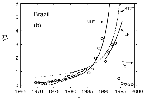
Since its inauguration in January 1985, the first democratic government after military rule exerted by the elected vice-president José Sarney (because the elected president Tancredo Neves fell ill) had limited means to resist spending pressure from congress. As a result, inflation, which had already been high for several years thanks to the old practice of monetary financing of budget deficits, frequent devaluations and indexation (automatic correction of prices, interest rates and wages according to past inflation), ran totally out of control. In 1987, the government was not able to pay the interest on its foreign debt and Brazil’s public debt had to be rescheduled. The inflation peaked at 2,950 $\%$ in 1990. This behavior can be seen in Fig. 1(b), where data of yearly GRI computed using values taken from a Table of the International Monetary Fund (IMF) imf are displayed. A new elected president Fernando Collor de Mello applied in 1990 the so-called Collor’s Plan in order to stop hyperinflation. As can be seen in Fig. 1(b) at the beginning the trend was changed, however, finally this plan for stabilization failed bresser91 ; merette00 .

The launch of the Plano Real in 1994 would prove to be the turning point. This plan, designed by Henrique Cardoso, who would later become Brazil’s president, envisaged the introduction of a new currency, put constraints on public spending and ended the indexation of the economy. The new currency, the real, had a crawling peg against the dollar as a nominal anchor and was somewhat overvalued, which made imports cheap, thus limiting the room for domestic producers to raise prices.

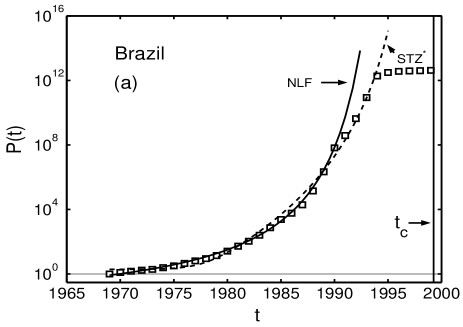
Sornette, Takayasu, and Zhou sornette03 have analyzed the complete series of CPI data from 1969 to 1994. The results from the fit of $P(t)$, instead of values of $\ln P(t)$, with the right-hand-side (r.h.s.) of expression (24) reported by STZ in Table 2 of Ref. sornette03 are quoted in Table 1 and displayed in Fig. 1(a). For the sake of completeness, we provide the relations between the parameters $\alpha$, $A$, and $B$ utilized by STZ and that used in the present work

$$r_{0}/\Delta t=\alpha\,B/(t_{c}-t_{0})^{1+\alpha}\;,$$ (26)

$$\beta=1/(1+\alpha)\;,$$ (27)

$$p_{0}=A+B/(t_{c}-t_{0})^{\alpha}\;.$$ (28)

We believe that the difficulty for fitting $\ln P(t)$ with Eq. (24) arises from the fact that in 1991 there is an important departure from the initial trend clearly depicted in Fig. 1(b). The applied theory with a unique value of $\beta$ is not able to describe the entire process. This feature is in agreement with the statement of Lucas lucas76 that parameters can change when economic policy changes. Therefore, in the present work we fitted to Eq. (24) the data of $\ln P(t)$ previous to 1991 only. Preliminary results have been already reported in Ref. szybisz10 . The numerical task was accomplished by using a routine of the book by Bevington bevington cited as the first reference in Chaps. 15.4 and 15.5 of the more recent Numerical Recipes press96 . In practice, the applied procedure yields the uncertainty in each parameter directly from the minimization algorithm. In order to quantify the contribution of the feedback we also evaluated $a_{p}$, which is given by [see Eq. (22)]

$$a_{p}=\frac{\Delta t}{\beta\,r_{0}^{\beta}\,(t_{c}-t_{0})}\;.$$ (29)

The obtained parameters, its uncertainties and the root-mean-square (r.m.s) residue of the fit, i.e. $\chi$, are quoted in Table 1. The determined $t_{c}$ is quite reasonable and the good quality of this fit may be observed in Fig. 1(a). The GRI was calculated by using Eq. (21) and displayed in Fig. 1(b), the theoretical results follows quite good the measured data. Vertical lines in both (a) and (b) panels indicate the obtained critical time $t_{c}$.

Figure 2: Squares are yearly CPI in Brazil from 1982 to 1998, normalized to $P(t_{0}=1969)=1$, presented in a semi-logarithmic. The solid curve NLF is the fit of $\ln P(t)$ from 1969 to 1990 with Eq. (24), while the solid curve LF stands for the fit of $\ln P(t)$ from 1990 to 1994 with Eq. (17). The dashed line is the fit of $P(t)$ reported by STZ* (see text).

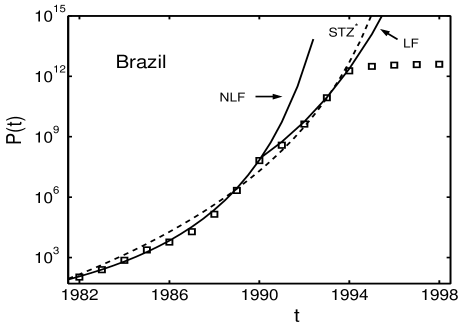
Figure 2 clearly shows a bifurcation between the trend of data from 1969 to 1990 and that of data from 1990 to 1994. Since there are only a few data points for the new incipient branch of hyperinflation, in order to have a quantitative description data of $r(t)$ and $\ln P(t)$ from 1990 to 1994 were simultaneously fitted with Eqs. (16) and (17), respectively. The obtained parameters are included in Table 1 and the fits denoted by LF are displayed in Figs. 1(b) and 2.

On the other hand, one may observe in Fig. 2 that the fit reported by STZ* does not follow quite well the set of measured CPI. The situation is even worse when one examine the GRI. According to the statement quoted on the top of page 499 of Ref. sornette03 the accumulated $P(t)$ is the exponential of the integral of $r(t)$ as expressed in Eq. (6) of the present work. The inverse, i.e. $r(t)$, becomes

$$r(t)=\frac{d\ln P(t)}{d(t/\Delta t)}=\frac{1}{P(t)}\,\frac{dP(t)}{d(t/\Delta t)}\;.$$ (30)

Assuming that $P(t)$ is given by Eq. (24) one gets

$$r(t)=\frac{r_{0}\,\left(\frac{t_{c}-t_{0}}{t_{c}-t}\right)^{1/\beta}}{p_{0}+\frac{r_{0}\,\beta}{1-\beta}\,\left(\frac{t_{c}-t_{0}}{\Delta t}\right)\biggr{[}\left(\frac{t_{c}-t_{0}}{t_{c}-t}\right)^{\frac{1-\beta}{\beta}}-1\biggr{]}}\;.$$ (31)

An evaluation of $r(t)$ by using this formula with the corresponding parameters quoted in Table 1 yielded the dashed curve depicted in Fig. 1(b). The theoretical curve oscillates between both branches of measured data. It is interesting to notice that the asymptotic form of Eq. (31) for $t\to t_{c}$ becomes

$$r_{asympt}(t)=\frac{1-\beta}{\beta}\,\left(\frac{\Delta t}{t_{c}-t}\right)\;,$$ (32)

yielding a universal singularity $(t_{c}-t)^{-1}$. This asymptotic regime is reached quite soon as shown by the dot-dashed curve in Fig. 1(b).

Table 2: Inflation in Nicaragua 1980-1997.

Year	Annual averaged $i(\%)$
	IMF-1a	IMF-2b
1980	35.1	35.1
1981	23.8	23.8
1982	24.9	28.5
1983	31.1	33.6
1984	35.4	141.3
1985	219.5	571.4
1986	681.0	885.2
1987	911.9	13109.5
1988	14315.8	4775.2
1989	4709.3	7428.7
1990	3127.5	3004.1
1991	7755.3	116.6
1992	40.5	21.9
1993	20.4	13.5
1994	7.7	3.7
1995	11.2	11.2
1996	11.6	11.6
1997	9.2	9.2

^a Data from IMF World Economic Outlook (WEO) imf .
^b Data from IMF (WEO) imf_2011 .

Let us now refer to the hyperinflation occurred in Nicaragua. During the decade of 1970’s this country was involved in a civil war. In 1979, the Sandinista National Liberation Front (FSLN) overthrew Anastasio Somoza Debayle, ending the Somoza dynasty, and established a revolutionary government in Nicaragua. This new government, formed in 1979 and dominated by the FSLN, applied a new model of economic development. The leader of this administration was Daniel José Ortega Saavedra (Sandinista junta coordinator 1979-85, president 1985-90).

Figure 3: (a) Squares are yearly CPI in Nicaragua from 1969 to 1997, normalized to $P(t_{0}=1969)=1$, presented in a semi-logarithmic plot. (b) Circles are yearly GRI in Nicaragua for the same period as in (a). The solid curve in (a) is the fit of $\ln P(t)$ from 1969 to 1987 with Eq. (24), NLF model, while the dashed curve is the fit including the value for 1988. The solid and dashed curves in (b) stand for $r(t)$ evaluated with Eq. (21) of the NLF model, for the shorter and longer series, respectively. In both drawings, the vertical lines indicate the corresponding values of $t_{c}$.

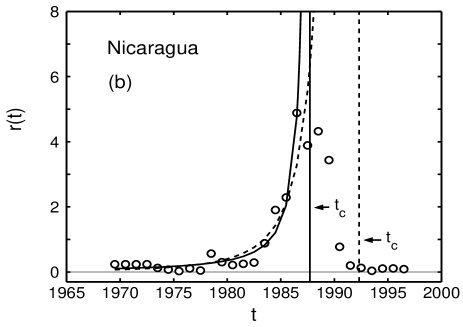
Economic growth was uneven in the 1980’s ocampo90 ; ocampo91 . After the end of the civil war the restructure and rebuild of the economy lead to a positive jump of GDP of about 5 percent in 1980 and 1981. However, each year from 1984 to 1990 showed a drop in the GDP. Reasons for the contraction included the reluctance of foreign banks to offer new loans, the diversion of funds to fight the new insurrection against the government hold by the Contras. Daniel Ortega began his six-year presidential term on January 1985, and established an austerity program to lower inflation. After the United States Congress turned down continued funding of the Contras in April 1985, the Reagan administration ordered a total embargo on United States trade with Nicaragua. The United States was formerly Nicaragua’s largest trading partner. The government spend a lot money to finance the war against the Contras during the second part of the 80’s decade. The gap between decreasing revenues and mushrooming military expenditures was filled by printing large amounts of paper money. Inflation skyrocketed, peaking at 13,109$\%$ percent annually at the end of 1987. In the last forty years, at Latin American level, this situation may be only compared with that occurred in Bolivia in 1985, where the value 11,150$\%$ was reached. So it sounds like pretty much the same story as many other hyperinflation events: War debts and foreign pressures inspire government to print large amounts of money. In 1988 began the efforts to stop the spiral of hyperinflation, however, the success of this attempt was very poor ocampo90 ; ocampo91 . It is worthwhile to notice that in the Nicaragua’s administration no Central Bank existed. In the February 1990 Violeta Barrios de Chamorro won the elections defeating Ortega. Afterwards, the usual stabilization procedures were rigorously applied leading to a stable regime in 1992.

Sornette et al. sornette03 analyzed the CPI from 1969 to 1991 evaluated with data taken from Ref. imf , the corresponding values of $i(t)$ for the regime close to the hyperinflation’s peak are listed in Table 2. Using the same procedure as that applied in the case of Brazil these authors fitted $P(t)$ instead of $\ln P(t)$ with Eq. (24). The obtained results are included in Table 1.

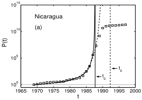
The inflation occurred in Nicaragua during the 1980’s decade is revisited in the present work. In so doing, we found revised data of $i(t)$ published by the IMF in the section of Economy in Ref. imf_2011 , which are also included in Table 2. A glance at this table indicates that the values at the beginning and at the end of both series are equal. However, the new values forming the peak of hyperinflation are shifted one year towards prior date and, in addition, the years corresponding to the values of about 7000$\%$ and 3000$\%$ are interchanged. The latter feature changes the profile of the crossover to the stationary regime. The CPI and GRI evaluated with data taken from Ref. imf_2011 are displayed in panels (a) and (b) of Fig. 3, respectively. The results plotted in Fig. 3(b) indicate that the inflation measured in 1989 can be assigned to the beginning of the decrease towards the stable regime. Therefore, we analyzed the hyperinflation using two sets of data, one considering values of CPI from 1969 to 1987 and the other including the value of 1988 also. This sort of fits yielded the parameters listed in Table 1. The solid curve in Fig. 3(a) indicates the fit of the shorter series to Eq. (24). A very steep slope of the CPI may be observed close to $t_{c}$. If the value of 1988 is included in the analysis, a piece of information on stabilization is taken into account, then the fit to Eq. (24) gives, as expected, a larger critical time. This value together with the other parameters and the $\chi$ are included in Table 1 and the fit is depicted by a dashed curve in Fig. 3(a). For both sets of parameters the GRI is evaluated with Eq. (21). The results are displayed in Fig. 3(b), where a good matching with measured data may be observed. In addition, in both panels of Fig. 3 the vertical lines stand for the determined values of $t_{c}$.

Figure 4: (a) Squares are yearly CPI in Israel since 1969 to 1991, normalized to P($t_{0}$=1969)=1, presented in a semi-logarithmic plot. The solid curve indicates the fit of $\ln P(t)$ since 1969 to 1985 to Eqs. (17) and (24) corresponding to the LF and NLF models, respectively, while the dashed curve stands for the fit of $P(t)$ to Eq. (24) as reported by STZ* (see text). (b) Circles are GRI for the same period as in (a). The solid curve was evaluated with Eqs. (16) and (21) provided by LF and NLF models, respectively, while the dashed curve was computed with Eq. (31) of the STZ* procedure (see text).

Figure 5: Squares are yearly CPI data in Israel since 1970 to 1989 taken as $\ln\ln[P(t)/P_{0}]$. The solid curve is the fit of data since 1969 to 1985 with the complete Eq. (17), while the dashed straight line is the asymptotic behavior of the LF model, i.e. $\ln\ln[P(t)/P_{0}]_{asympt}$, given by Eq. (36).

III.2 A drawback of the NLF model: Israel

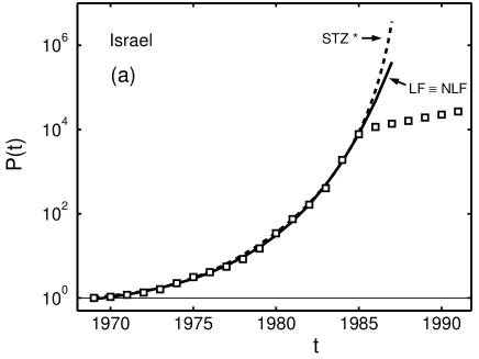
Let us now focus on the case of Israel. The difficulties for determining a reasonable $t_{c}$ from data of this country have a different origin from those found in the cases of Brazil and Nicaragua. Figure 4(a) shows the yearly data for the CPI in Israel computed using data taken from a Table of the International Monetary Fund (IMF) imf . The evolution of this CPI may be summarized as follows. Deterioration of the internal and external conditions following the energy crisis and the Yom Kippur War of 1973 led to an increase in inflation. The labor government chose to accommodate it in the same way as Brazil. The single-digit rates of inflation in the 1960’s, developed to an annual inflation rate of about $40\%$ in 1974-75, about $80\%$ in 1978, and got triple-digit rates of about $400\%$ at their peak in the mid-1980’s. Leiderman and Liviatan leiderman03 attributed this response to the implicit preference for short-term considerations of avoiding unemployment over long-term monetary stability. In 1985 a new strategy was applied that combines drastic cuts in government deficit and fixed nominal variables (anchors), i.e. the exchange rate, wages and bank credit. This approach succeeded in bringing down inflation to a moderate level (near $10\%$). In the 90’s inflation targeting was adopted and inflation came down to levels recommended by the Organization for Economic Cooperation and Development (OECD), i.e., about 2 or $3\%$.

The hyperinflation since 1969 to 1985 clearly exhibits a faster than exponential growth as indicated by the upward curvature of the logarithm of CPI as a function of time displayed in Fig. 4(a). In a first step, we fitted data of CPI to Eq. (24) in a similar way to that performed by STZ sornette03 . The obtained parameters and the $\chi$ are listed in Table 1. A glance at this table indicates a critical time $t_{c}=2061$ and a small exponent of the power law $\beta=0.069$ ($\alpha\simeq 13$). According to STZ sornette03 both these values are unrealistic for a developing hyperinflation, in addition, they state that the results are not improved by reducing the time intervals over which the fits are performed. In addition, they attributed these problems to the fact that the later prices close to the end of the time series start to enter a cross-over to a saturation.

Furthermore, the values $t_{c}=2061\pm 72$ and $\beta=0.069\pm 0.061$, which agree with that mentioned by STZ sornette03 , were obtained by stopping the minimization procedure when the variation of $\chi^{2}$ between the $i+1$ and $i$ iterations was smaller than a standard choice $10^{-1}\,\%$. However, if one allows to continue the iterations a correlation between these both parameters becomes clear, $t_{c}$ increases while $\beta$ decreases approaching zero, this happens in such a way that the product $\beta\times(t_{c}-t_{0})$ converges to a constant yielding a well defined value of the parameter $a_{p}$ given by Eq. (29). For instance, in Table 1 we quoted values obtained when the change of $\chi^{2}$ becomes less than $10^{-3}\,\%$.

Let us now show that by following the route $\beta\to 0$ described by numerical minimization the NLF expressions for GRI and CPI converge to Eqs. (16) and (17) derived in the MTT’s LF model mizuno02 , which corresponds to set $\beta=0$ in Eq. (19). The expression for $r(t,\beta\to 0)$ is obtained starting from Eq. (21)

$$r(t,\beta\to 0) = r_{0}\,\lim_{\beta\to 0}\,\biggr{[}\frac{1}{1-\beta\,a_{p}\,r_{0}^{\beta}\left(\frac{t-t_{0}}{\Delta t}\right)}\biggr{]}^{1/\beta}$$ (33)

$$= r_{0}\,\lim_{\beta\to 0}\,\biggr{[}\frac{1}{1-\beta\,a_{p}\,\left(\frac{t-t_{0}}{\Delta t}\right)}\biggr{]}^{1/\beta}\;.$$

It is noteworthy that after the change of variable $\beta=q-1$ the last expression can be identify with the limit $q\to 1$ of the q-exponential function, i.e. $e^{x}_{q}$, used in studies of nonextensive statistical mechanics and economics tsallis03

$$r(t,\beta\to 0) = r(t,q\to 1)$$ (34)

$$= r_{0}\,\lim_{q\to 1}\,\biggr{[}\frac{1}{1-(q-1)\,a_{p}\,\left(\frac{t-t_{0}}{\Delta t}\right)}\biggr{]}^{1/(q-1)}$$

$$= r_{0}\,\lim_{q\to 1}\,\biggr{[}e_{q}^{[a_{p}\,(t-t_{0})/\Delta t]}\,\biggr{]}$$

$$= r_{0}\,\exp\biggr{[}a_{p}\,\left(\frac{t-t_{0}}{\Delta t}\right)\biggr{]}\;,$$

because $e_{1}^{x}=e^{x}$ (see Ref. tsallis03 ). Furthermore, imposing the limit $\beta\to 0$ in Eq. (LABEL:lptn) for CPI one gets

$$p(t,\beta\to 0)=p_{0}$$

$$+\lim_{\beta\to 0}\,\biggr{\{}\frac{r_{0}^{1-\beta}}{(1-\beta)\,a_{p}}\biggr{(}\biggr{[}\frac{1}{1-\beta\,a_{p}\,r_{0}^{\beta}\left(\frac{t-t_{0}}{\Delta t}\right)}\biggr{]}^{\frac{1-\beta}{\beta}}-1\biggr{)}\biggr{\}}$$

$$=p_{0}+\frac{r_{0}}{a_{p}}\biggr{\{}\lim_{\beta\to 0}\biggr{[}\frac{1}{1-\beta\,a_{p}\,r_{0}^{\beta}\left(\frac{t-t_{0}}{\Delta t}\right)}\biggr{]}^{\frac{1}{\beta}}-1\biggr{\}}$$

$$=p_{0}+\frac{r_{0}}{a_{p}}\,\biggr{\{}\exp\biggr{[}a_{p}\,\left(\frac{t-t_{0}}{\Delta t}\right)\biggr{]}-1\biggr{\}}\;.$$ (35)

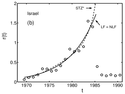
The results obtained in Eqs. (34) and (35) are equal to the corresponding formulas of the LF model. Therefore, we also fitted the CPI data for the period 1969-1985 directly with LF’s Eq. (17). The obtained parameters together with the r.m.s residue $\chi$ are included in Table 1. The good quality of the fit may be observed in Fig. 4(a). Notice the excellent agreement between the values of $r_{0}$, $a_{p}$, and $\chi$ yielded by the LF approach and those obtained from the “long” fit with Eq. (24) of the NLF model. Both these fits are equivalent as indicated in Fig. 4(a). It is also worthwhile to mention that the present value for the parameter utilized in the MTT description, i.e. $B_{MTT}=1+2a_{p}=1.35$, is in good agreement with the result $1.4$ quoted in Table 1 of Ref. mizuno02 . For the sake of completeness we plotted in Fig. 4(b) the measured data of GRI together with the theoretical values yielded by Eqs. (16) and (21) provided by LF and NLF models, respectively.

The analysis was completed by fitting data of CPI from 1969 to 1984, i.e. stopping the series before the imposition of the final stabilization. The results are also included in Table 1, no sizable differences from the fits to the larger series were observed.

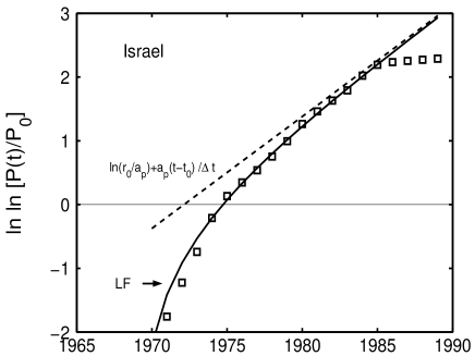
The success of the LF’s description in the case of Israel is due to the fact that a double-exponential law is an upper bound for data of $P(t)$. This feature is depicted in Fig. 5, where measured values of $\ln\ln P(t)$ are plotted together with the fit with the complete LF model and the straight line given by the asymptotic expression of this model

$$\ln\ln\biggr{[}\frac{P(t)}{P_{0}}\biggr{]}_{asympt}=\ln\biggr{(}\frac{r_{0}}{a_{p}}\biggr{)}+a_{p}\,\biggr{(}\frac{t-t_{0}}{\Delta t}\biggr{)}\;.$$ (36)

One may realize that experimental data of the hyperinflation (i.e. until 1985) approach the asymptotic straight line from bellow.

Although the LF model provides a good fit, it does not predict any $t_{c}$ indicative for a possible crash of the economy. In order to estimate a $t_{c}$, the authors of Ref. sornette03 adopted the same trick as that used in the cases of Brazil and Nicaragua, i.e., fitting data of $P(t)$, rather than values of $\ln P(t)$, with the r.h.s. of Eq. (24). The results reported in Table 2 of Ref. sornette03 are included in the present Table 1 and the fit is shown in Fig. 4(a). For the sake of completeness, $r(t)$ was calculated using Eq. (31) corresponding to the STZ* choice and displayed in Fig. 4(b)). However, this procedure for overhauling the lack of a theoretical tool able to account for any degree of saturation does not preserve the logical structure of the entire model. As emphasized above, $P(t)$ is the exponential of the integral of $r(t)$ as given by Eq. (6). In this case $r(t)$ would be given by Eq. (31). In turn, this expression for $r(t)$ should be obtained as a solution of a differential equation, e.g. Eq. (LABEL:rate00), which must be formulated in a dynamical description of this kind of economic system. The latter requirement is not fulfilled in the analysis performed by STZ*, hence, it remains as a simple fit to a selected expression only.

IV Summary and Conclusions

In the present work we treated regimes of hyperinflation in economy. The episodes occurred in Brazil, Israel, and Nicaragua were revisited. These new studies indicated that after some management of data outlined in Sec. III.1 the cases of Brazil and Nicaragua were successfully described within the frame of the NLF model available in the literature sornette03 ; szybisz09 . This formalism outlined in Sec. II.2 is based on a nonlinear feedback characterized by an exponent $\beta>0$, see Eq. (LABEL:rate00). In this model, a critical time $t_{c}$ at which the economy would blow up can be determined from a finite time singularity of the form $1/(t_{c}-t)^{(1-\beta)/\beta}$ exhibited by the CPI.

It was found that the hyperinflation occurred in Brazil from 1969 to 1994 can be satisfactorily well described within the NLF frame if one assumes that, in fact, there are two successive regimes: one from 1969 to 1990 previous to the Collor’s Plan and the other subsequent to that plan. For the first regime a reasonable $t_{c}$ was obtained. This feature is in agreement with the statement of Lucas lucas76 , that parameters can change once policy changes.

On the other hand, the episode developed in Nicaragua can be well described when the corrected data are considered. The corrections of the inflation series reported in the literature are centered around the peak of the data. The corrected values yielded a reasonable $t_{c}$ within the frame of the NLF model.

Finally, by applying the NLF model to the weaker hyperinflation of Israel no $t_{c}$ is got. Moreover, the data are consistent with $\beta\to 0$ and, in turn, this limit leads to the linear feedback proposed in Ref. mizuno02 which does not predict any $t_{c}$. In this case there is neither bifurcation of CPI nor correction of data, instead, there is a slowly increasing hyperinflation due to a permanent but incomplete effort to stop inflation.

Since it would be of interest to estimate a $t_{c}$ within a self-consistent theory even in the case of a weak hyperinflation, we shall propose in a forthcoming work an extension of the NLF model including the effect of a latent incomplete stabilization. This purpose will be achieved by introducing a new parameter acting on all past $r(t)$.

Let us finish emphasizing that these lessons should not be lost, but instead should be kept in mind to avoid the repetition of that unpleasing experiences. Moreover, one should always remain the statement of Keynes keynes30 , namely that: “even the weakest government can enforce inflation when it can enforce nothing else”.