Cosmological stealths with nonconformal couplings

Abstract

In this paper we reconsider the existence of stealth fields during the evolution of our Universe by admitting more realistic nonminimal couplings to gravity than the conformal one. In the framework of the FRW cosmology we found that inhomogeneous stealths, as those enabled in the conformal case, are only allowed in de Sitter backgrounds. In particular, it is shown that the homogeneous stealths resulting from nonconformal couplings can coexist with each kind of matter dominant in the several phases characterizing the evolution of our Universe according to the $\Lambda$CDM model.

I Introduction

The standard cosmological model describes the evolution of an isotropic and homogeneous universe as required by the cosmological principle, that is of a spacetime described by the Friedmann-Robertson-Walker (FRW) metric

$$ds^{2}=a(\tau)^{2}\left(-d\tau^{2}+\frac{dr^{2}}{1-kr^{2}}+r^{2}\left(d\theta^{2}+\sin^{2}\!\theta\,{d}\phi^{2}\right)\right),$$ (1)

where $\tau$ is the conformal time and $a(\tau)$ is the scale factor. The constant $k$ determines the spatial topology of the Universe, with $k=-1,0,+1$ corresponding to open, flat and closed universes. For a given matter content $\varphi_{\text{m}}$, metric (1) extremizes the action

$$S[g,\varphi_{\text{m}}]=\int{d}^{4}x\sqrt{-g}\left(\frac{1}{2\kappa}(R-2\Lambda)+L_{\text{m}}\right),$$ (2)

by solving Einstein equations

$$G_{\mu\nu}+\Lambda g_{\mu\nu}-\kappa{T}_{\mu\nu}=0\,,$$ (3)

where $\kappa$ is the Einstein constant and $\Lambda$ is the cosmological constant. A consistent picture of the cosmological history, supported by the observational data Bernabei:2014ema ; Suzuki:2011hu ; Dawson:2012va ; Aghanim:2015xee , emerged from the corresponding solutions of (3). Known as the Big Bang, it describes an early very flat universe filled with a quark-gluon plasma which started to expand and to get colder, giving rise to many phase transitions in the matter content. This picture involves a mixture of fluids, however, since the density of each fluid varies differently with the expansion, there are long periods of time where the energy of a given fluid is dominant while the other ones are subdominant. This way, the early radiation dominated phase was replaced, about $350000$ years later, by an intermediate era dominated by pressureless matter (baryonic and of an unknown kind coined dark). By the end of the last century it was empirically established that very recently our observable universe became dominated by some energy (also of an unknown kind and also coined dark) doing a positive work which induces accelerated expansion. The simplest candidate for this dark energy is a positive cosmological constant.

All of the above mentioned cosmological phases can be modeled with barotropic perfect fluids given by an equation of state $p=w\rho$, where $p$ and $\rho$ stand, correspondingly, for the pressure and energy density of the fluid, while $w$ is the constant of state. In absence of a cosmological constant, the solution of Einstein equations (3) for the flat FRW universe (1) filled with a barotropic fluid corresponds to a power law (see Appendix A)

$$a(\tau)=a_{b}\tau^{b},\qquad b\equiv\frac{2}{1+3w}.$$ (4)

For radiation, $w=1/3$, the power is $b=1$, while for baryonic and dark pressureless matter, $w=0$, it is $b=2$. Even more, the case of a universe dominated by the cosmological constant can also be described by (4) with a constant of state $w=-1$. As it was mentioned, the corresponding solution with $b=-1$ is accelerating and is known as the de Sitter spacetime.

Since the described background is homogeneous and isotropic, the picture briefly drawn cannot explain the existence of cosmic large scales structures, which are the consequence of the growth of primordial density fluctuations. Amongst some other problems, it neither explains why our Universe looks so flat, given that, with a positive constant of state, the flat case is an unstable equilibrium of the cosmological dynamics Liddle:2000cg ; Mukhanov:2005sc . Up to date, the best available solution to these problems is called cosmological inflation Liddle:2000cg ; Mukhanov:2005sc . It also describes an accelerated expansion, but at very early times, even before the formation of the quark-gluon plasma. The cosmological constant is not a good candidate for the inflationary matter because the de Sitter universe is unstable in the sense that it never ends to accelerate, thus not giving place to the rise and expansion of the quark-gluon plasma. Therefore, perhaps the simplest scenario is that of the energy density in the very early universe being dominated by the potential energy of a single real scalar field $\phi$ called inflaton. Then, the quantum fluctuations of the inflaton served as the seeds for the formation of large scale structure and of the anisotropies in the cosmic microwave background (CMB). An interesting model is power-law inflation for potential $V(\phi)\propto\exp(-\sqrt{2\kappa(b+1)/b}\,\phi)$ and scale factor (4) with $b<-1$ Lucchin:1984yf . It has several attractive features concerning theory and observations Liddle:2000cg ; Mukhanov:2005sc . First, the tree expansions often used for scalar field potentials arising in quantum field theory are just deviations from the truncated Taylor series of the exponential function. Second, the exponential potential is the only inflationary model yielding exact power-law spectra Abbott:1984fp , and because the departure of the spectra amplitudes from scale invariance is predicted to be very small, the power-law parametrization of the primordial spectra is often used while analyzing the CMB data Aghanim:2015xee .

This whole description of the evolution of our Universe is known as the $\Lambda$ cold dark matter ($\Lambda$CDM) model. Data from highly accurate satellite and ground-based observations strongly support this model as the best theoretical framework Aghanim:2015xee . Nevertheless, in spite of the success of the $\Lambda$CDM model, there is still a large number of open questions in cosmology, perhaps the more relevant being what is the nature of most of the matter content of our Universe. We do not know what are the dark energy, the dark matter or the precise inflationary matter. Typically, candidates for these kinds of matter are accepted or discarded considering the impact they have on the behavior of the scale factor, which in turn determines the values of most cosmological observables. Additionally, a less known kind of exotic matter can also be included in the $\Lambda$CDM model. It has been shown that General Relativity allows for special nontrivial matter configurations with no backreaction on the gravitational field, i.e. whose existence does not affect the evolution of the underlying spacetime. Scalar fields with this property were first found for the static BTZ black hole AyonBeato:2004ig and later for the Minkowski flat space AyonBeato:2005tu , (A)dS space AyonBeato:SAdS and other holographic backgrounds Ayon-Beato:2015qfa . They were coined gravitational stealths. The existence of stealths for the de Sitter (dS) cosmology was studied in Ref. Banerjee:2006pr . The relevance they have for the probability of nucleation of such universes was emphasized in Ref. Maeda:2012tu .

Moreover, in Ref. Ayon-Beato:2013bsa it was shown that not only de Sitter universes, but any homogeneous and isotropic universe, independently of its spatial topology and matter content, allows for the presence of a conformal stealth which evolves along with the Universe without exhibiting its gravitational fingerprints. This result can be understood as a mapping of the previously known stealth configurations of Minkowski spacetime into stealths in FRW spacetimes. The corresponding map was found using the conformal symmetry of the stealth action, as well as the conformal flatness of FRW spacetime which is a consequence of its homogeneity and isotropy. Nevertheless, as it was already mentioned, the later are just approximated symmetries of the actual Universe where stars, galaxies, clusters of galaxies, etc. are present. Therefore, many important observables of the successful $\Lambda$CDM model are related to density perturbations which grew into this cosmic large scale structure. The backreaction of these density perturbations, on the one hand breaks the above mentioned symmetries of the FRW spacetimes, spoiling its conformal flatness, and on the other hand they also induce perturbations on the coexisting conformal stealth. These last perturbations differ from the stealth in nature because they are necessarily coupled both to the matter sources, which were never conformally invariant, and to the perturbed spacetime which is not longer conformally flat. Consequently, conformal symmetry is irrelevant at the perturbative level defining the $\Lambda$CDM model. Hence, constraining the stealths of cosmology to being conformally coupled is an unnecessary restriction which can severely limit the analysis of more realistic scenarios. For this reason, the main motivation of this paper is to explore the existence of stealth configurations in FRW spacetimes for general nonminimal couplings, where no obvious conformal arguments can be used.

In the next section we state the problem for a general nonminimal coupling parameter $\xi$ and derive the relevant expressions. One main conclusion is that going beyond the conformal coupling, $\xi\neq 1/6$, necessarily implies that a generic cosmology only allows homogeneous stealths. In contrast with the conformal case, $\xi=1/6$, the only exception are just the de Sitter cosmologies. In Sec. III we first show the existence of a class of stealths during a big bang era for generic values of $\xi$. Later we present some examples of stealth potentials for different couplings during those eras of the $\Lambda$CDM model when the matter content was dominated by the energy of a single fluid as those yielding (4). Next, in Sec. IV the inhomogeneous stealths of the de Sitter cosmologies are analyzed in detail for generic values of the nonminimal coupling parameter. The special value of the coupling $\xi=1/4$ is studied in Sec. V. For homogeneous stealths the nonminimal coupling to gravity can be reinterpreted as contributing to the self-interaction of the field; the arising of this effective self-interaction potentials is discussed in Sec. VI. In the last section we briefly summarize our conclusions. We also include some appendixes with relevant details.

II Stealths with nonconformal couplings

Let us start here by stating the problem of finding stealth scalar fields not necessarily conformally coupled to the FRW spacetime (1). With this aim we supplement action (2) with the one describing a self-interacting scalar field $\Psi$ nonminimally coupled to gravity

$$S[g,\varphi_{\mathrm{m}}]-\int{d}^{4}x\sqrt{-g}\left(\frac{1}{2}\partial_{\mu}\Psi\partial^{\mu}\Psi+\frac{\xi}{2}R\Psi^{2}+U(\Psi)\right),$$ (5)

where $\xi$ is the nonminimal coupling parameter, and the special value $\xi=1/6$ is the one describing the conformal case. Next, we demand the first term to be again extremized by solving Einstein equations (3) for the same matter content $\varphi_{\mathrm{m}}$. This necessarily implies that the second term does not contribute to the extrema, i.e. the corresponding energy-momentum tensor must vanish on the background,

$$0=T^{\mathrm{s}}_{\mu\nu}={} \partial_{\mu}\Psi\partial_{\nu}\Psi-g_{\mu\nu}\left(\frac{1}{2}\partial_{\alpha}\Psi\partial^{\alpha}\Psi+U(\Psi)\right)$$

$$+\xi\left(g_{\mu\nu}\square-\nabla_{\mu}\nabla_{\nu}+G_{\mu\nu}\right)\Psi^{2}\,,$$ (6)

and any nontrivial solution $\Psi$ to the above constraint defines a stealth configuration.

In order to find these nontrivial solutions on a given FRW background with scale factor $a$ it is useful to redefine the field as

$$\Psi=\frac{1}{\sqrt{\kappa}\left(a\sigma\right)^{\frac{2\xi}{1-4\xi}}},$$ (7)

where the function $\sigma=\sigma(x^{\mu})$ inherits the full spacetime dependence of the scalar field. This redefinition is chosen because it allows to follow the general method used in Ayon-Beato:2013bsa for the conformal case. From now on the nonminimal coupling parameter $\xi$ is taken to be nonvanishing (because there is no stealth for minimal coupling $\xi=0$) and different from the value $\xi=1/4$, which will be studied in Sec. V.

Hence, following Ayon-Beato:2013bsa we conclude, by solving the off-diagonal components of the stealth constraint (6), that the redefined field is again separable according to

$$\sigma(x^{\mu})=T(\tau)+R(r)+r\left[\Theta(\theta)+\sin(\theta)\Phi(\phi)\right].$$ (8)

This separation is defined up to a residual symmetry; homogeneous terms in $\Phi$, $\Theta$, and $R$ can be compensated by a sinusoidal dependence in $\Theta$, a linear one in $R$, and another homogeneous term in $T$, respectively.

Now, by taking differences of the diagonal components of (6), it is found that as in Ayon-Beato:2013bsa

$$\Phi(\phi) =A_{1}\cos\phi+A_{2}\sin\phi,$$ (9a)

$$\Theta(\theta) =A_{3}\cos\theta,$$ (9b)

$$R(r) =\left\{\begin{array}[]{ll}B_{-}\sqrt{1-kr^{2}},&k\neq 0,\\ \\ \frac{1}{2}\alpha{r}^{2},&k=0,\end{array}\right.$$ (9f)

where the above mentioned residual symmetry has been taken into account. Here, $A_{i}$ ($i=1,2,3$), $\alpha$ and $B_{-}$ are integration constants whose dimensions are inverse length.

The remaining difference of diagonal components is

$$0 =\frac{(1-4\xi)a^{2}\sigma}{4\xi^{2}\Psi^{2}}\left(T_{~{}\theta}^{\mathrm{s}~{}\theta}-T_{~{}\tau}^{\mathrm{s}~{}\tau}\right)$$

$$=\begin{cases}T^{\prime\prime}+kT+\dfrac{3}{\xi}\left(\xi-\dfrac{1}{6}\right)\left(\mathcal{H}^{\prime}-\mathcal{H}^{2}-k\right)\sigma,&k\neq 0,\\ \\ T^{\prime\prime}+\alpha+\dfrac{3}{\xi}\left(\xi-\dfrac{1}{6}\right)\left(\mathcal{H}^{\prime}-\mathcal{H}^{2}\right)\sigma,&k=0,\end{cases}$$ (10)

where $\mathcal{H}\equiv a^{\prime}/a$ is the conformal Hubble parameter and the prime denotes derivatives with respect to conformal time. Is here where the first differences with respect to the approach of Ref. Ayon-Beato:2013bsa appear. In that reference, the inhomogeneous $\sigma$ contributions of conditions (10) do not appear because the studied coupling had the conformal value $\xi=1/6$. This allowed us to find exactly the time dependent contribution $T$, regardless of the scale factor $a$ and the corresponding spatial dependence of the stealth. This is no longer valid for the general nonminimal couplings, $\xi\neq 1/6$, considered here. As can be appreciated from (10), the stealth must be necessarily homogeneous, unless the parentheses including the conformal Hubble parameter vanishes, i.e.

$$\mathcal{H}^{\prime}-\mathcal{H}^{2}-k=0.$$ (11)

Only when the above constraint is fulfilled inhomogeneous configurations having $\sigma(x^{\mu})\neq T(\tau)$ are allowed, independently of the value taken by the nonminimal coupling parameter. Constraint (11) has a single solution which is precisely the de Sitter universe (Appendix D), whose inhomogeneous stealths will be studied in Sec. IV. In other words, it follows from (10) that the only cosmologies allowing inhomogeneous stealths for a generic value of the nonminimal coupling parameter $\xi\neq 1/6$ are the de Sitter ones. For any other cosmology it is necessarily satisfied that $\sigma(x^{\mu})=T(\tau)$, i.e. the resulting stealths become homogeneous, which according to (8) only occurs when all the integration constants appearing in solution (9) vanish. Summarizing, in order to completely determine the stealth from expression (7) for a nonconformal coupling and a given scale factor (defining a cosmology different from the de Sitter one), it remains to find the extra time dependence from Eqs. (10). For arbitrary backgrounds, no general closed-form solution exists for these equations, i.e. it will depend on the specific form of the scale factor.

After solving (10), we would have satisfied all the off-diagonal conditions of the stealth constraint (6), as well as all the differences between the diagonal ones. Hence, only one last condition needs to be satisfied, which fixes the unique potential defining the self-interacting behavior of the stealth. For a generic cosmology this condition is

$$0=-T_{~{}\tau}^{\mathrm{s}~{}\tau}={} U(\Psi)-\frac{\Psi^{2}}{2a^{2}}\biggl{\{}6\xi\left[(6\xi-1)\mathcal{H}^{2}-k\right]$$

$$\qquad\qquad\qquad-\left[\left(\ln{a^{6\xi}\Psi}\right)^{\prime}\right]^{2}\biggr{\}}.$$ (12)

In the next section we start by finding the explicit form of the nonconformal stealths for the scale factors which describe the different eras of $\Lambda$CDM cosmology.

III Stealths in $\Lambda$CDM Cosmology

Perhaps the more interesting solution to the problem stated in the previous section is a stealth witnessing the whole cosmological evolution as described by the $\Lambda$CDM model. In principle, the solution on the related background can be found by numerically integrating (10), however, for a better understanding of the main features of this universal stealth it is useful to do the analysis for each of the eras comprising the $\Lambda$CDM model.

With this aim we start by analyzing the Big Bang era. As it was already mentioned, it describes the evolution of the mixture of two kinds of barotropic perfect fluids: radiation and pressureless matter. Let $\rho_{\mathrm{\nu}}$ and $\rho_{\mathrm{m}}$ be the densities for radiation and matter respectively, then (as is explicitly shown in Appendix B) one can solve for the scale factor as

$$a(\tau)=a_{1}\tau+a_{2}\tau^{2},$$ (13a)

where

$$a_{1}=\sqrt{\frac{3}{\kappa\rho_{\mathrm{\nu}}}},\quad a_{2}=2\sqrt{\frac{3}{\kappa\rho_{\mathrm{m}}}},$$

and the powers are fixed according to (4). With this scale factor, the homogeneous solution of Eq. (10) for $k=0$ is given in terms of the hypergeometric function

$$T(\tau)={} a(\tau)^{\frac{1}{2}-\beta_{1}}$$

$$\times\!\biggl{[}C_{1}\;{}_{2}F_{1}\!\!\left(\gamma_{-}-2\beta_{1},\gamma_{+}-2\beta_{1};1-2\beta_{1};-\frac{a_{2}}{a_{1}}\tau\right)$$

$$+C_{2}\tau^{2\beta_{1}}\,_{2}F_{1}\!\!\left(\gamma_{-},\gamma_{+};1+2\beta_{1};-\frac{a_{2}\tau}{a_{1}}\right)\biggr{]},$$ (14a)

where

$$\beta_{1}=\sqrt{\frac{25}{4}-\frac{1}{\xi}},\quad\gamma_{\pm}=\frac{1}{2}\pm\sqrt{\frac{73}{4}-\frac{3}{\xi}},$$ (14b)

and $C_{1}$, $C_{2}$ are integration constants. Recall that to find the self-interaction potential we need to solve the constraint (II). The usual way to deal with this problem is to write the explicit dependence of both the stealth and the scale factor on the coordinates (in this case $\tau$) and then use the inverse relation between the stealth and the coordinates to exhibit the explicit dependence $U(\Psi)$. However, relation (7) is not invertible in general for an arbitrary nonminimal coupling $\xi$. This is the case for the scale factor (13a).

In spite of the above difficulty we can outline the main properties of these stealths if we use the fact that initially ($\tau<<1$) the first contribution in the scale factor (13a) dominates, indicating a radiation phase, and lately ($\tau>>1$) the leading term is the second one, corresponding to a matter dominated phase. This way in each case the scale factor is reduced to just a power-law. Even more, as mentioned in the Introduction, another important phase of the $\Lambda$CDM cosmology which is also described by a power-law is inflation. Taking into account all these reasons, we will consider a power-law evolution in flat universes as described by the scale factor (4). After introducing this expression in the stealth condition (10) we obtain the following differential equation

$$\tau^{2}T^{\prime\prime}-\frac{3b(b+1)(\xi-1/6)}{\xi}T=0.$$ (15)

This is an Euler equation and their linearly independent solutions are also power-laws, $T\propto\tau^{\gamma}$, whose exponents $\gamma$ are determined from the corresponding characteristic polynomial

$$\gamma^{2}-\gamma-\frac{3b(b+1)(\xi-1/6)}{\xi}=0,$$ (16)

solved by

$$\gamma_{\pm} =\frac{1}{2}\pm\sqrt{\Delta}\,,$$ (17a)

$$\Delta =\frac{b(b+1)}{2}\left(\frac{1}{\xi_{b}}-\frac{1}{\xi}\right),$$ (17b)

$$\xi_{b} =\frac{1}{6+\frac{1}{2b(b+1)}}.$$ (17c)

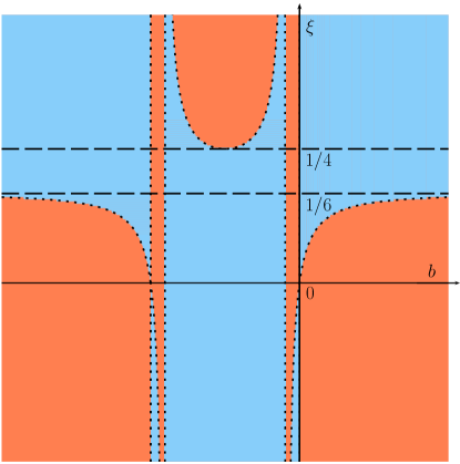
Figure 1: Regions where the discriminant $\Delta$ is positive (light blue) and negative (salmon).

Therefore, the precise functional form of the solutions of the Euler equation (15) depends on the sign of the discriminant $\Delta$. These signs can be appreciated in Fig. 1, where the blue regions denote $\Delta>0$, the salmon ones $\Delta<0$ and consequently $\Delta=0$ are just the boundaries between these regions. We analyze each of these cases in the following subsections.

III.1 Solutions with $\Delta>0$

The discriminant (17b) is positive for two general cases: the first, when $-1<b<0$ with $\xi<\xi_{b}$, and the second, for $b>0$ or $b<-1$ with $\xi>\xi_{b}$ (see Fig. 1). In those cases the general solution of the Euler equation (15) is given by

$$T(\tau)=A_{0}\tau^{\frac{1}{2}+\beta}+\sigma_{0}\tau^{\frac{1}{2}-\beta},$$ (18a)

where $$A_{0} \sigma_{0}$$ and are integration constants and

$$\beta=\sqrt{\Delta}\,.\\$$ (18b)

Using this solution the stealth field (7) can be expressed as

$$\Psi(\tau)=\Psi_{0}\left[\left(\frac{\tau}{\tau_{0}}\right)^{b+\frac{1}{2}+\beta}+\left(\frac{\tau}{\tau_{0}}\right)^{b+\frac{1}{2}-\beta}\right]^{\frac{-2\xi}{1-4\xi}},$$ (19a)

where the new constants are related to the old ones by

$$\tau_{0}= \left(\frac{\sigma_{0}}{A_{0}}\right)^{\frac{1}{2\beta}},$$ (19b)

$$\Psi_{0}= \frac{1}{\sqrt{\kappa}}\left[a_{0}\sigma_{0}^{\frac{b+\frac{1}{2}+\beta}{2\beta}}A_{0}^{-\frac{b+\frac{1}{2}-\beta}{2\beta}}\right]^{\frac{-2\xi}{1-4\xi}}.$$ (19c)

In general, expression (19a) is not invertible and the corresponding self-interaction potential must be parametrically given by

$$U(\Psi)=\left\{\begin{array}[]{ll}\Psi(\tau),\\ U(\tau),\end{array}\right.$$

where $U(\tau)$ is given by (II).

It is worthy to notice that the relation between $\tau$ and $\Psi$ can be inverted for some specific values of the powers of $\tau$ that appear in (19a); this fixes either the scale factor exponent $b$ or the nonminimal coupling parameter $\xi$. Now we proceed to study two of these explicit examples.

III.1.1 Explicit potential for fixed scale factor exponent

The first explicit example is obtained by choosing the exponent as $b=-1/2$ and $\xi<1/4$, since (19a) becomes

$$\Psi(\tau)=\frac{\Psi_{0}}{\left[\left(\frac{\tau}{\tau_{0}}\right)^{\hat{\beta}}+\left(\frac{\tau}{\tau_{0}}\right)^{-\hat{\beta}}\right]^{\frac{1}{4\hat{\beta}^{2}}}},$$ (20)

which is inverted as

$$\tau=\tau_{0}\left(\frac{1\pm\sqrt{1-4\left(\frac{\Psi}{\Psi_{0}}\right)^{8\hat{\beta}^{2}}}}{2\left(\frac{\Psi}{\Psi_{0}}\right)^{4\hat{\beta}^{2}}}\right)^{\frac{1}{\hat{\beta}}},$$ (21)

where the dependence on the nonminimal coupling parameter is encoded in

$$\hat{\beta}=\sqrt{\frac{1-4\xi}{8\xi}}.$$ (22)

Therefore, it is possible to obtain the two families of potentials

$$U_{\pm}(\Psi)={} \frac{2^{\frac{1}{\hat{\beta}}}U_{0}}{16\hat{\beta}^{2}(2\hat{\beta}^{2}+1)}\left(\frac{\Psi}{\Psi_{0}}\right)^{2(2\hat{\beta}+1)}\frac{1}{\left[1\pm P(\Psi)\right]^{2+\frac{1}{\hat{\beta}}}}$$

$$\times\left[2(2\hat{\beta}+1)[3(2\hat{\beta}+1)\pm 2(\hat{\beta}+1)P(\Psi)]\rule{0.0pt}{17.07164pt}\right.$$

$$\times\left(\frac{\Psi}{\Psi_{0}}\right)^{8\hat{\beta}^{2}}-8(2\hat{\beta}^{2}+1)\left(\frac{\Psi}{\Psi_{0}}\right)^{16\hat{\beta}^{2}}$$

$$\left.{}-(2\hat{\beta}+1)(4\hat{\beta}+1)\left[1\pm P(\Psi)\right]\rule{0.0pt}{17.07164pt}\right],$$ (23a)

with

$$P(\Psi)\equiv\sqrt{1-4\left(\frac{\Psi}{\Psi_{0}}\right)^{8\hat{\beta}^{2}}},\quad U_{0}=\frac{\Psi_{0}\,^{2}}{16\tau_{0}a_{0}\,^{2}}.$$ (23b)

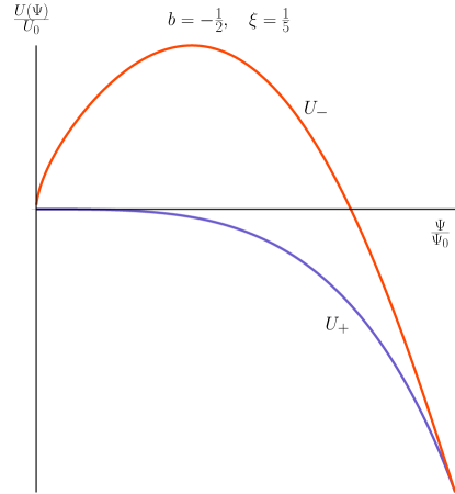
Figure 2: The self-interaction potentials of the stealth overflying a power-law universe with exponent $b=-1/2$ are plotted for $\xi=1/5$.

As an illustration, the plot of the two branches $U_{+}(\Psi)$ and $U_{-}(\Psi)$ with $\xi=1/5$ is presented in Fig. 2.

III.1.2 Explicit potential for fixed nonminimal coupling

For the second explicit example, we fix the nonminimal coupling parameter in terms of the exponent of the scale factor by

$$\xi=\tilde{\xi}\equiv\frac{9b(b+1)}{4[13b(b+1)+1]},$$ (24)

which cover the two general cases described at the beginning of this subsection that give a positive discriminant (17b). Concretely, in the first case the value $b=-1/2$ and the following intervals are excluded

$$-\frac{1}{2}-\frac{3}{2\sqrt{13}} <b<-\frac{1}{2}-\frac{1}{\sqrt{6}},$$

$$-\frac{1}{2}+\frac{1}{\sqrt{6}} <b<-\frac{1}{2}+\frac{3}{2\sqrt{13}},$$

since the defining condition $\tilde{\xi}<\xi_{b}$ is only satisfied for the rest of the interval $-1<b<0$. All the values of the second case are covered by the parametrization (24), because $\tilde{\xi}>\xi_{b}$ for $b<-1$ and $b>0$.

After fixing the nonminimal coupling, expression (19a) becomes

$$\Psi(\tau) =\frac{\Psi_{0}}{\left[\left(\frac{\tau}{\tau_{0}}\right)^{2\tilde{\beta}}+\left(\frac{\tau}{\tau_{0}}\right)^{\tilde{\beta}}\right]^{\frac{18\tilde{\beta}^{2}-1}{16\tilde{\beta}^{2}}}},$$ (25a)

$$\tilde{\beta} =\frac{2b+1}{3}.$$ (25b)

For $b\neq-1/2$, this relation allows the inversion

$$\tau=\tau_{0}\left[\frac{-1+\sqrt{1+4\left(\frac{\Psi_{0}}{\Psi}\right)^{\frac{16\tilde{\beta}^{2}}{18\tilde{\beta}^{2}-1}}}}{2}\right]^{\frac{1}{\tilde{\beta}}}.$$ (26)

Hence, the allowed potential is given by

$$U(\Psi)={} \frac{2^{\frac{1}{\tilde{\beta}}+2}U_{0}(9\tilde{\beta}^{2}-1)^{2}}{\tau_{0}\,^{6\beta}\tilde{\beta}^{2}(13\tilde{\beta}^{2}-1)}\left(\frac{\Psi}{\Psi_{0}}\right)^{2}\left[Q(\Psi)-1\right]^{\frac{1}{\tilde{\beta}}-3}$$

$$\times\left\{[Q(\Psi)-1](13\tilde{\beta}^{2}-1)\left(\frac{\Psi}{\Psi_{0}}\right)^{\frac{16\tilde{\beta}^{2}}{9\tilde{\beta}^{2}-1}}\right.$$

$$+2\left[2(13\tilde{\beta}^{2}+3\tilde{\beta}-1)Q(\Psi)-21\tilde{\beta}^{2}-6\tilde{\beta}+3\right]$$

$$\times\left(\frac{\Psi}{\Psi_{0}}\right)^{\frac{8\tilde{\beta}^{2}}{9\tilde{\beta}^{2}-1}}\left.-\frac{8(1+\tilde{\beta})(3\tilde{\beta}^{2}+4\tilde{\beta}-1)}{3\tilde{\beta}+1}\right\}$$ (27a)

where

$$Q(\Psi)\equiv\sqrt{1+4\left(\frac{\Psi}{\Psi_{0}}\right)^{\frac{8\tilde{\beta}^{2}}{1-9\tilde{\beta}^{2}}}},$$ (27b)

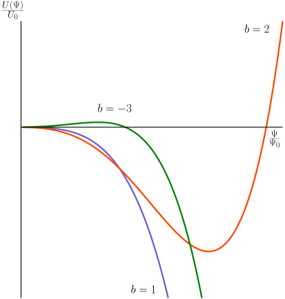
Figure 3: The second example of an explicit self-interaction potential for the stealth is plotted for radiation, $b=1$, matter, $b=2$, and inflation with $b=-3$.

and $U_{0}$ is still defined as in (23b). In Fig. 3 we plot the potentials for interesting power laws corresponding to phases dominated by matter, radiation, and a case of inflation.

III.1.3 Early/late time approximation for arbitrary exponent and coupling

For a generic phase characterized by a power-law exponent $b$ the stealth potential cannot be explicitly obtained for an arbitrary value of the nonminimal coupling parameter $\xi$. Nevertheless, we can approximate the stealth solution for both early and late times in a given phase. The resulting approximations turn out to be invertible giving the effective potentials characterizing the self-interaction of the stealth in the corresponding evolution regimes. Using the notations $\Psi_{-}(\tau)=\Psi(\tau\ll\tau_{0})$ and $\Psi_{+}(\tau)=\Psi(\tau\gg\tau_{0})$ then both cases can be summarized within the same expression

$$\Psi_{\pm}(\tau)=\Psi_{0}\left(\frac{\tau}{\tau_{0}}\right)^{-\frac{\xi\left(2b+1\pm 2\beta\right)}{1-4\xi}}.$$ (28)

The explicit self-interaction potential for each approximation is

$$U(\Psi_{\pm})=\lambda_{\pm}\left(\frac{\Psi_{\pm}}{\Psi_{0}}\right)^{\frac{2[1-3\xi+(1-2\xi)b\pm 2\xi\beta]}{\xi(2b+1\pm 2\beta)}},$$ (29a)

where the self-interaction coupling constants are given by

$$\lambda_{\pm}={} -\frac{16U_{0}\xi}{\tau_{0}\,^{2b+1}(4\xi-1)^{2}}\left\{\pm 2\xi[1+4(6\xi-1)b]\beta\right.$$

$$\left.{}+(6\xi-1)[2(8\xi-1)b+4\xi+1]b+\xi\right\}.$$ (29b)

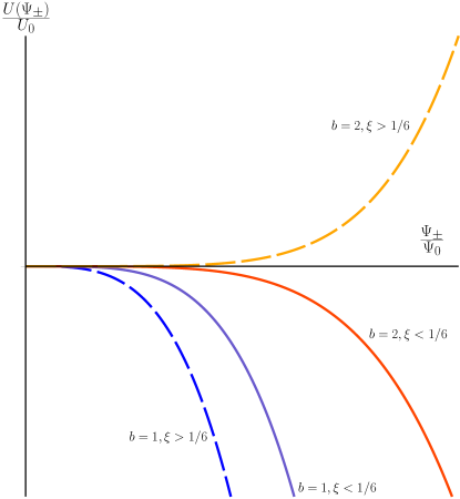
Figure 4: Stealth self-interaction for different phases of the early universe and values of the nonminimal coupling parameter $\xi$. The blue line, $U(\Psi_{+})$ corresponds to the late time radiation dominated epoch, $b=1$, and the red line $U(\Psi_{-})$ to the early matter dominated phase, $b=2$. The graphs with $\xi<1/6$ are drawn with solid lines while for $\xi>1/6$ have long dash lines.

We present in Fig. 4 plots for two particular cases, the late time approximation of the radiation dominated phase, $b=1$, and the early time approximation of the matter dominated phase, $b=2$, for different values of the nonminimal coupling parameter $\xi$. With these cases we end the discussion of solutions with positive discriminant $\Delta$.

Summarizing the results in this subsection, we have found different explicit solutions for the stealth problem when the discriminant (17b) is positive. We have obtained the self-interaction potentials by fixing, on the one hand, the value of the scale factor exponent and, on the other hand, the nonminimal coupling parameter in terms of the former. We covered relevant phases of the Universe evolution, moreover, early and late time regimes of these phases were also explicitly addressed. Several behaviors of the potentials were found depending on the election of the nonminimal coupling parameter and the scale factor exponent. Particularly, we have found cases where the obtained potentials are unbounded from below, however this behavior can be mended as will be discussed in Sec. VI. In the following subsection we proceed to study solutions with negative discriminant.

III.2 Solutions with $\Delta<0$

As it is shown in Fig. 1, the discriminant $\Delta$ given by (17b) will be negative when $-1<b<0$ with $\xi>\xi_{b}$, or in the case when $b>0$ or $b<-1$ with $\xi<\xi_{b}$. Therefore, the power exponents of the solutions to the Euler equation (15) become imaginary, leading to trigonometric dependences. Consequently, for $\Delta<0$ the stealth field can be expressed as

$$\Psi(\tau)=\Psi_{0}\left[\left(\frac{\tau}{\tau_{0}}\right)^{b+1/2}\cos\left(\sqrt{-\Delta}\ln\frac{\tau}{\tau_{0}}\right)\right]^{-\frac{2\xi}{1-4\xi}}.$$ (30)

Once again, if $b=-1/2$ ($\xi>1/4$) it is possible to give an explicit solution, since the relation between the stealth and the conformal time can be inverted as

$$\tau =\tau_{0}\exp\left\{\frac{1}{\overline{\beta}}\arccos\left[\left(\frac{\Psi}{\Psi_{0}}\right)^{4\overline{\beta}^{2}}\right]\right\},$$ (31)

$$\overline{\beta} =\sqrt{\frac{4\xi-1}{8\xi}}.$$ (32)

Therefore, the functional form of the potential is

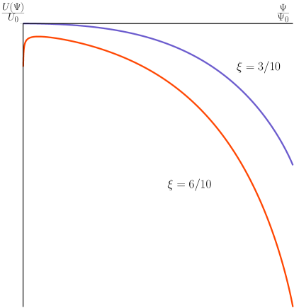
Figure 5: Homogeneous stealth self-interaction of the oscillatory solution with $b=-1/2$ for two values of $\xi>1/4$.

$$U(\Psi)={} 4U_{0}\exp\left\{-\frac{1}{\overline{\beta}}\arccos\left[\left(\frac{\Psi}{\Psi_{0}}\right)^{4\overline{\beta}^{2}}\right]\right\}\left(\frac{\Psi}{\Psi_{0}}\right)^{2}$$

$$\times\left[\frac{1-2\overline{\beta}^{2}}{2\overline{\beta}^{2}}\left(\frac{\Psi}{\Psi_{0}}\right)^{-8\overline{\beta}^{2}}+\frac{1+2\overline{\beta}^{2}}{2\overline{\beta}^{2}}\rule[5.69054pt]{0.0pt}{22.76219pt}\right.$$

$$+\left.\frac{3}{\overline{\beta}}\sqrt{\left(\frac{\Psi}{\Psi_{0}}\right)^{-8\overline{\beta}^{2}}-1}\,\rule[5.69054pt]{0.0pt}{22.76219pt}\right].$$ (33)

The plots of this potential are shown in Fig. 5.

In this subsection we have studied the case were the discriminant (17b) is negative and, as in the previous subsection, an explicit solution for the stealth and its self-interaction was found upon fixing the scale factor exponent. It only remains to analyze the case with vanishing discriminant in the next subsection.

III.3 Solutions with $\Delta=0$

We can appreciate from definition (17b) that a vanishing discriminant corresponds to the value of nonminimal coupling $\xi=\xi_{b}$, implying that the Euler equation (15) has a single root with multiplicity two and the stealth can be found to be

$$\Psi(\tau)=\Psi_{0}\left[\left(\frac{\tau}{\tau_{0}}\right)^{b+\frac{1}{2}}\ln\frac{\tau}{\tau_{0}}\right]^{\frac{-4b(b+1)}{(2b+1)^{2}}}.$$ (34)

Is not possible to obtain explicitly the potential in this case since this relation is not invertible. Nevertheless, we can have an idea of the stealth potential in presence of radiation or matter by plotting it parametrically after fixing the corresponding exponent $b$. They exhibit a similar behavior to the potential $U_{+}$ of Fig. 2.

Here, we exhaust the scanning of nonconformal stealths in universes with power-law scale factor. Their necessarily homogeneous behavior is a characteristic on all FRW universes, except for the de Sitter ones that we study in the following section.

IV de Sitter cosmologies with inhomogeneous stealths

In Sec. II it was concluded that, except for the conformal coupling $\xi=1/6$, the stealths of a generic universe must be necessarily homogeneous, which are precisely the ones studied in the previous section. The only exceptions allowing inhomogeneous stealths are the universes satisfying the constraint (11). As it is proved in Appendix D this constraint unambiguously defines the de Sitter universes

$$ds^{2}=\frac{l^{2}k}{\sin^{2}\sqrt{k}\tau}\left(-d\tau^{2}+\frac{dr^{2}}{1-kr^{2}}+r^{2}d\Omega^{2}\right).$$ (35)

For them, even though the nonminimal coupling is not conformal, condition (10) lead us to the same time dependence obtained for the stealth in the conformal case Ayon-Beato:2013bsa , that is

$$T(\tau)=\begin{cases}\dfrac{A_{0}}{\sqrt{k}}\sin\sqrt{k}\tau+B_{+}\cos\sqrt{k}\tau,&k\neq 0,\\ -\frac{1}{2}\alpha\tau^{2}+A_{0}\tau+\sigma_{0},&k=0,\rule{0.0pt}{17.07164pt}\end{cases}$$ (36)

where $A_{0}$, $B_{+}$ and $\sigma_{0}$ are integration constants. This allows us to write the full dependence of the auxiliary function characterizing the stealth as

$$\sigma(x^{\mu})={} \frac{A_{0}}{\sqrt{k}}\sin\sqrt{k}\tau+\left(\frac{\sigma_{0}}{2}+\frac{\alpha}{k}\right)\cos\sqrt{k}\tau$$

$$+\left(\frac{\sigma_{0}}{2}-\frac{\alpha}{k}\right)\sqrt{1-k\,\vec{x}^{2}}+\vec{A}\cdot\vec{x}.$$ (37)

Here, the integration constants have been redefined as $B_{\pm}=\sigma_{0}/2\pm\alpha/k$. Let us remind that the spatial integration constants $A_{1},A_{2},A_{3}$ can be set to zero through quasitranslations as it was done in Ref. Ayon-Beato:2013bsa . Finally, having the explicit dependence of the stealth, we can find analytically the self-interaction potential by solving constraint (II) which gives

$$U_{dS}(\Psi)={} \frac{2\xi\Psi^{2}}{(1-4\xi)^{2}}\Big{[}\xi\lambda_{1}(\sqrt{\kappa}\Psi)^{\frac{1-4\xi}{\xi}}$$

$$+24\lambda_{2}\xi(\xi-1/6)(\sqrt{\kappa}\Psi)^{\frac{1-4\xi}{2\xi}}$$

$$-\frac{48}{l^{2}}(\xi-1/6)(\xi-3/16)\Big{]},$$ (38a)

where the coupling constants are defined by

$$\lambda_{1} =A_{\mu}A^{\mu}-2\alpha\sigma_{0},$$ (38b)

$$\lambda_{2} =A_{0}/l.$$ (38c)

This is exactly the self-interaction found in Ref. AyonBeato:SAdS for the stealth on the dS background as is reviewed in Appendix E.

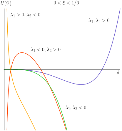
Figure 6: Stealth self-interaction in de Sitter cosmologies for different values of the coupling constants when $0<\xi<1/6$.

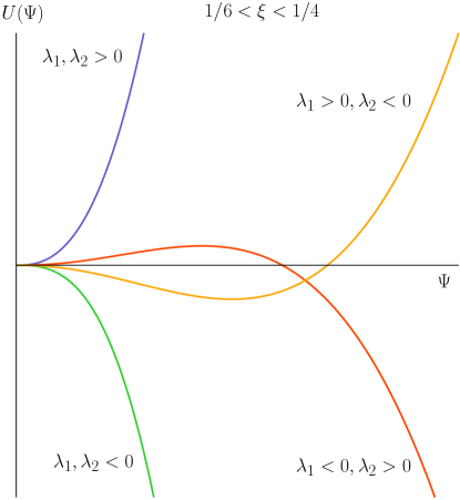
Figure 7: Stealth self-interaction in de Sitter cosmologies for different values of the coupling constants when $1/6<\xi<1/4$.

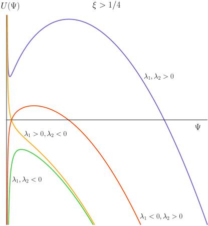
Figure 8: Stealth self-interaction in de Sitter cosmologies for different values of the coupling constants when $\xi>1/4$.

For $\xi=1/6$ this potential becomes the conformal one already studied in Ref. Ayon-Beato:2013bsa and exhibiting a single global minimum. Whereas for $\xi\neq 1/6$, the existence of their extrema depends on the values of the coupling constants $\lambda_{1}$ and $\lambda_{2}$. For example, if $\lambda_{1}>0$, $\lambda_{2}>0$ and $0<\xi<1/6$ the potential has a local maximum at $\Psi=0$ and a global minimum (see Fig. 6). Conversely, for $1/6<\xi<1/4$ there is only a global minimum at $\Psi=0$ for the same range of coupling constants, as is shown in Fig. 7 along with other possible values for the couplings. Similarly, the cases with $\xi>1/4$ are plotted in Fig. 8 showing an unbounded from below potential for all values of the couplings. However, these undesired behaviors might be corrected when the nonminimal coupling contribution is seen as part of the field self-interaction in its equation of motion. This will be studied in detail in Sec.VI.

Up to now, all our analysis rest on the redefinition (7) which excludes the value $\xi=1/4$ of the nonminimal coupling. In the following section we analyze how to handle this particular coupling.

V Nonminimal coupling $\xi=1/4$

Finally, in this section we address the atypical behavior of the stealth for the coupling $\xi=1/4$, where its relation with the auxiliary function (7) is no longer valid. In this case the pertinent redefinition is

$$\Psi=\frac{\exp{(a\sigma)}}{\sqrt{\kappa}},$$ (39)

which allows the function $\sigma(x^{\mu})$ to remain separable exactly the same as it was before [see Eqs. (8) and (9)]. This way, the only dependence still to be determined is the temporal one, which is rigged again by the combination (10) which changes now to

$$0 =-\frac{2a}{\Psi^{2}}\left(T_{~{}\theta}^{\mathrm{s}~{}\theta}-T_{~{}\tau}^{\mathrm{s}~{}\tau}\right)$$

$$=\begin{cases}T^{\prime\prime}+kT+\left(\mathcal{H}^{\prime}-\mathcal{H}^{2}-k\right)\left(\sigma+\dfrac{1}{a}\right),&k\neq 0,\\ \\ T^{\prime\prime}+\alpha+\left(\mathcal{H}^{\prime}-\mathcal{H}^{2}\right)\left(\sigma+\dfrac{1}{a}\right),&k=0.\end{cases}$$ (40)

As for any other coupling different from the conformal one, the solutions to these equations are simplified for de Sitter cosmologies, giving rise to inhomogeneous stealths to be studied in subsection V.2. For any other cosmology the stealth has to be homogeneous, $\sigma(x^{\mu})=T(\tau)$. In the next subsection, motivated by the $\Lambda$CDM model, we will consider the case of a power-law scale factor in a flat universe.

V.1 Homogeneous stealth: power-law scale factor

In a flat universe, $k=0$, with power-law scale factor $a(\tau)=a_{0}\tau^{b}$ the equations determining the temporal dependence of the stealth (40) become again the Euler equation (15) for $\xi=1/4$ but with an additional power-law inhomogeneity

$$\tau^{2}T^{\prime\prime}-b(b+1)T=\frac{b(b+1)}{a_{0}}\tau^{-b},$$ (41)

whose solutions are now

$$T(\tau)=\begin{cases}A_{0}\tau^{b+1}+\tau^{-b}\left(\sigma_{0}-\frac{b(b+1)}{a_{0}(2b+1)}\ln\tau\right),&b\neq-\frac{1}{2},\\ \\ \sqrt{\tau}\left(A_{0}+\sigma_{0}\ln\tau-\frac{1}{8a_{0}}\ln^{2}\tau\right),&b=-\frac{1}{2}.\end{cases}$$ (42)

The corresponding stealth, which must be derived in these cases using the redefinition (39), is not invertible for generic values of the scale factor exponent. Nevertheless, again the exponent $b=-1/2$ is an exception yielding

$$\Psi(\tau)=\Psi_{0}\exp\left(-\frac{1}{8}\ln^{2}\frac{\tau}{\tau_{0}}\right),$$ (43a)

where the integration constants are rewritten as

$$\tau_{0} =\exp(4a_{0}\sigma_{0}),$$ (43b)

$$\Psi_{0} =\frac{1}{\sqrt{\kappa}}\exp\left[a_{0}(A_{0}+2a_{0}\sigma_{0}^{2})\right],$$ (43c)

which allows to invert the conformal time as

$$\tau=\tau_{0}\exp\left(\pm 2\sqrt{2\ln\frac{\Psi_{0}}{\Psi}}\right).$$ (44)

Hence, the resulting self-interaction potential is

$$U(\Psi)={} -\frac{U_{0}\Psi^{2}}{\Psi_{0}^{2}}\exp\left(-2\sqrt{2\ln\frac{\Psi_{0}}{\Psi}}\right)$$

$$\times\left(4\ln\frac{\Psi_{0}}{\Psi}+6\sqrt{2\ln\frac{\Psi_{0}}{\Psi}}+3\right),$$ (45)

where the constant $U_{0}$ is again given as in (23b). Potentials with similar qualitative behavior have been observed in previous sections. For $b\neq-1/2$ the corresponding potentials can only be obtained parametrically. In particular, this allows to verify that the plots for the cases of matter and radiation are also similar to others presented in previous figures.

V.2 Inhomogeneous stealth: de Sitter cosmologies

As it was emphasized after Eq. (40), inhomogeneous stealths can only be present in de Sitter cosmologies. To obtain them for $\xi=1/4$ we could proceed analogously as we did in Sec. IV for the other nonconformal couplings, i.e. to straightforwardly derive and solve the equations for the temporal dependence of the stealth and to use this knowledge to determine the potential. Nevertheless, for de Sitter universes these equations are the same regardless of the value of $\xi$ and consequently the auxiliary function $\sigma(x^{\mu})$ remains unchanged. As it was shown in Ref. Ayon-Beato:2015qfa the exponential dependence present in redefinition (39) for $\xi=1/4$ arises as a nontrivial limit of the definition (7) for the auxiliary function corresponding to generic values of the coupling. We believe it is more enlightening to exploit here this approach to find the $\xi=1/4$ potential as a nontrivial limit of (38a).

The starting point of the procedure introduced in Ref. Ayon-Beato:2015qfa is to consider the following limit

$$\lim_{\xi\to 1/4}\frac{2\xi(1-a(\tau)\sigma(x^{\mu}))}{1-4\xi}\equiv a(\tau)\hat{\sigma}(x^{\mu}).$$ (46)

If it is well behaved, modulo redefinitions of the integration constants, a new auxiliary function could be defined according to the above right-hand side. Then, starting from the expression for a generic coupling (7), configuration (39) can be reached as the nonminimal coupling goes to the value $\xi=1/4$, i.e.

$$\Psi =\lim_{\xi\to 1/4}\frac{1}{\sqrt{\kappa}}\left(a\sigma\right)^{-\frac{2\xi}{1-4\xi}}$$

$$=\lim_{\xi\to 1/4}\frac{1}{\sqrt{\kappa}}\left(1-\frac{1-4\xi}{2\xi}a\hat{\sigma}+\mathcal{O}\left((1-4\xi)^{2}\right)\right)^{-\frac{2\xi}{1-4\xi}}$$

$$=\frac{\exp(a\hat{\sigma})}{\sqrt{\kappa}}.$$ (47)

In the present case, the condition (46) is achieved for the stealth solution (37) on de Sitter cosmologies (35) by redefining the integrations constants as

$$A_{0} =\frac{1}{l}-\frac{1-4\xi}{2\xi}\hat{A}_{0},$$ (48a)

$$\left(\sigma_{0},\alpha,\vec{A}\right) =-\frac{1-4\xi}{2\xi}\left(\hat{\sigma}_{0},\hat{\alpha},\vec{\hat{A}}\right),$$ (48b)

which allows to obtain exactly the same expression for the new auxiliary function in terms of the new integration constants

$$\hat{\sigma}(x^{\mu})={} \frac{\hat{A}_{0}}{\sqrt{k}}\sin\sqrt{k}\tau+\left(\frac{\hat{\sigma}_{0}}{2}+\frac{\hat{\alpha}}{k}\right)\cos\sqrt{k}\tau$$

$$+\left(\frac{\hat{\sigma}_{0}}{2}-\frac{\hat{\alpha}}{k}\right)\sqrt{1-k\,\vec{x}^{2}}+\vec{\hat{A}}\cdot\vec{x}.$$ (49)

The next step is to obtain the $\xi=1/4$ potential as the limit resulting from considering the redefinitions (48) on the starting self-interaction (38a), which after a careful rearrangement can be rewritten as follows:

$$U(\Psi)={} \lim_{\xi\to 1/4}-\frac{\Psi^{2}}{2l^{2}}\left[\left(1+\mathcal{O}(1-4\xi)\right)\rule{0.0pt}{19.91692pt}\right.$$

$$\times\left(\frac{\Psi^{\frac{1-4\xi}{2\xi}}-1}{\frac{1-4\xi}{2\xi}}-\hat{A_{0}}l+\frac{3}{2}+\mathcal{O}(1-4\xi)\right)^{2}$$

$$\left.\rule{0.0pt}{19.91692pt}-\hat{\lambda}_{1}-\frac{3}{4}+\mathcal{O}(1-4\xi)\right]$$

$$={} -\frac{\Psi^{2}}{2l^{2}}\Bigg{[}\left(\ln\frac{\Psi}{\Psi_{0}}+\frac{3}{2}\right)^{2}-\hat{\lambda}_{1}-\frac{3}{4}\Bigg{]},$$ (50a)

where the new coupling constants are

$$\hat{\lambda}_{1} =l^{2}[\vec{\hat{A}}-2\hat{\alpha}\hat{\sigma}_{0}],$$ (50b)

$$\Psi_{0} =\frac{\exp(\hat{A}_{0}l)}{\sqrt{\kappa}}.$$ (50c)

Expressions (V.2) and (50) are just the exact ones obtained by straightforwardly integrating the stealth constraints for the nonminimal coupling $\xi=1/4$. These results are in agreement with those previously found for (A)dS in Ref. AyonBeato:SAdS . The obtained potential has extrema at

$$\Psi_{\pm}=\Psi_{0}\exp\left(-2\pm\sqrt{1+\hat{\lambda}_{1}}\right),$$ (51)

which are local minima or maxima depending on the particular choices for $\hat{\lambda}_{1}$. Different configurations are plotted in Fig. 9.

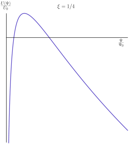
Figure 9: Stealth self-interaction in de Sitter cosmologies when the nonminimal coupling has the special value $\xi=1/4$.

VI Stealth effective potential

In previous sections we stated the problem of finding the stealth potential in different cases. Particularly, we were able to determine the potential as an explicit function of the field when the dependence of the stealth on the conformal time was invertible. Nevertheless, it is important to notice that to fully understand the stealth dynamics it must be considered that due to the nonminimal coupling to gravity there is a term that can be considered as part of an effective potential. Recall that the field equation of motion is

$$\Box\Psi=U^{\prime}(\Psi)+\xi R\Psi,$$ (52)

which is obtained by taking the variation of action (5) with respect to the stealth. In a universe driven by a barotropic perfect fluid, by taking the trace of the Einstein equations (3), using the conserved density (59) and the resulting power law (62) we obtain

$$R=\frac{2\kappa(b-1)}{b}\rho=\frac{6b(b-1)}{a_{b}^{2}}\frac{1}{\tau^{2(b+1)}},$$ (53)

i. e., the Ricci scalar is proportional to the density of the fluid. As a result, when the conformal time is invertible in terms of the stealth, $\tau=\tau(\Psi)$, the scalar curvature can be expressed as a local function of this scalar field, allowing to rewrite its equation of motion (52) as follows

$$\Box\Psi=U_{\text{eff}}^{\prime}(\Psi).$$ (54)

Hence, the effective potential is defined as

$$U_{\text{eff}}(\Psi)\equiv U(\Psi)+\frac{6{\xi}b(b-1)}{a_{b}^{2}}\int{\frac{\Psi}{\tau(\Psi)^{2(b+1)}}d\Psi}.$$ (55)

Let us consider as nontrivial examples the particular cases of the early and late time approximations studied in subsubsection III.1.3. For them, the inversion of their homogeneous stealths (28) in terms of the conformal time gives power-law behaviors, which after being considered in the integration of the nonminimal contribution of (55), leads to the same exponents appearing in their original potentials (29). Consequently the effective potentials are

$$U_{\text{eff}}(\Psi_{\pm})=\lambda_{\pm}^{\text{eff}}\left(\frac{\Psi_{\pm}}{\Psi_{0}}\right)^{\frac{2[1-3\xi+(1-2\xi)b\pm 2\xi\beta]}{\xi(2b+1\pm 2\beta)}},$$ (56a)

where the correction is manifested via the related coupling constants

$$\lambda_{\pm}^{\text{eff}}\equiv\lambda_{\pm}+\frac{48\xi^{2}(2b+1\mp 2\beta)b(b-1)U_{0}}{[b+1-\xi(2b+3)\mp 2\xi\beta]\tau_{0}\,^{2b+1}}.$$ (56b)

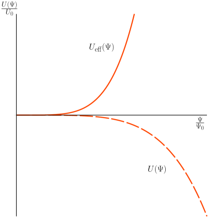
Figure 10: The potential in presence of matter with $b=2$ is unbounded from below when $\xi<1/6$, however considering the correction due to the nonminimal coupling turns it well behaved.

In some cases, like for instance stealths in presence of matter ($b=2$) with a nonminimal coupling $\xi<1/6$, the self-interaction constants can change its sign, drastically modifying the behavior of the potential as can be seen in Fig. 10.

VII Conclusions and outlook

The aim of the current work was to show that the $\Lambda$CDM model admits a wider class of stealth fields than those conformally coupled to gravity already studied in Ref. Ayon-Beato:2013bsa . The motivation behind this plan is that most observables of this cosmological model are determined not only by the time dependence of the scale factor but also by the evolution of acoustic oscillations of density perturbations around the time when radiation and matter densities were nearly equal. The introduction of the density perturbations into the picture implies to break both the conformal flatness of the FRW universe and the conformal symmetry of the stealth action considered in Ayon-Beato:2013bsa ; the two indispensable ingredients justifying the existence of the conformal stealths. Hence, the answer to the question on the presence of stealths in the $\Lambda$CDM model necessarily implies dealing with nonconformal couplings to gravity.

For more general nonminimal couplings we found in this research that inhomogeneous stealths, as those enabled in the conformal case, are only allowed in de Sitter backgrounds. Therefore, the $\Lambda$CDM stealth has to be unavoidably homogeneous. We were able to find a version of such nonconformal stealth by restricting the problem to a FRW universe filled with radiation and matter. Unfortunately, the corresponding expression for this stealth as function of the conformal time is given in terms of hypergeometric functions, which makes it almost impossible to explicitly find the corresponding self-interaction potential. The analogous task for the whole $\Lambda$CDM model is even more challenging, but it could be approached numerically. Moreover, an idea of how the potential for the $\Lambda$CDM stealth would look can be drawn by solving the problem taking into account that in each epoch of the cosmological evolution the corresponding scale factor has a given power-law dependence on the conformal time. Here, we solved the problem for homogeneous stealths during power-law inflation, radiation and matter dominated eras, and during de Sitter expansion, which are the main epochs of the $\Lambda$CDM model. We obtained a variety of functional forms for the stealth potential, which may or may not be modified after considering the contribution accounting for the nonminimal coupling to gravity in the stealth equation of motion. For certain combinations of the nonminimal coupling $\xi$ and the scale-factor exponent $b$ this effective potential bounds the stealth dynamics, in some cases allowing for the possibility of a stealth which evolves towards a minimum in any of the main epochs of the $\Lambda$CDM model.

There are two interesting and complementary ways of extending the results in this paper to look for observational consequences of the existence of the $\Lambda$CDM stealth. First of all, one can now consider the cases where neither the stealth action is conformally invariant nor the spacetime is conformally flat. This will allow us to establish whether a stealth field can exist on inhomogenous or anisotropic universes like, for instance, several of the Bianchi spacetimes. Complementarily, one can take the usual approach of considering that the actual universe is well approximated by FRW plus small perturbations. Using now the several examples of stealths found here and the interesting fact that their fluctuations are not necessarily stealth themselves, it would be possible to explore their consequences on the spectra of the cosmic microwave background radiation and in the cosmological large-scale structures statistics.

Appendix A Scale factor for barotropic fluids in conformal time

As emphasized in the Introduction all cosmological phases can be modeled by their dominant barotropic perfect fluid which imposes a power-law behavior for the scale factor. Since this fact is intensively used the paper we summarize here how it is described in terms of the conformal time. This allows us to fix the notation for the remaining Appendixes and the whole paper.

A perfect fluid satisfies the continuity equation

$$\rho^{\prime}+3\mathcal{H}(\rho+P)=0.$$ (57)

This fluid is denominated barotropic if additionally respects the equation of state

$$P=w\rho,$$ (58)

which allows to integrate the continuity equation, yielding the following relation between the scale factor and the density

$$\rho =\rho_{0}\left(\frac{a}{a_{b}}\right)^{-2(b+1)/b},$$ (59a)

where

$$b=\frac{2}{3w+1},\qquad a_{b}=|b|\left(\frac{3}{\kappa\rho_{0}}\right)^{1/2},$$ (59b)

and the last is a length scale defined by the integration constant density $\rho_{0}$. Using the above density (59) on the Friedmann equation

$$3\mathcal{H}^{2}=\kappa\rho a^{2}-3k,$$ (60)

for the flat case $k=0$ (which is the most interesting from the observational point of view Aghanim:2015xee ) it becomes

$$\left(\frac{a^{\prime}}{a_{b}}\right)^{2}=b^{2}\left(\frac{a}{a_{b}}\right)^{2(b-1)/b}.$$ (61)

This equation is easily integrated yielding

$$a(\tau)=a_{b}\tau^{b},$$ (62)

modulo redefinitions of the conformal time making it positive in all cases. This is the scale factor characterizing the conformal time evolution of a barotropic perfect fluid and the starting point of the following two Appendixes.

Appendix B Scale factor for a mixture of radiation and matter

The first examples of stealths analyzed in Sec. III are those present in the big bang era, which is characterized by the evolution of a mixture of radiation ($w=1/3$) and pressureless matter ($w=0$). We explicitly describe here the simultaneous evolution of these two kinds of barotropic perfect fluids. Interestingly, in spite of the nonlinearity that Friedmann equation (60) inherits from Einstein equations, the resulting scale factor reduces to a superposition of those each fluid obeys separately. For a mixture of radiation, $b=1$, and matter, $b=2$,

$$\rho=\rho_{\nu}+\rho_{\mathrm{m}},$$ (63)

since each component is individually conserved, their corresponding densities (59) will be

$$\rho_{\nu}=\rho_{\nu 0}\left(\frac{a}{a_{1}}\right)^{-4},\quad\rho_{\mathrm{m}}=\rho_{\mathrm{m}0}\left(\frac{a}{a_{2}}\right)^{-3}.$$ (64)

Using these expressions, the flat Friedmann equation (60) reduces to

$$(a^{\prime})^{2}=4a_{2}a+(a_{1})^{2},$$ (65)

which can be straightforwardly integrated as

$$a(\tau)=a_{2}(\tau-\tau_{0})^{2}-\frac{(a_{1})^{2}}{4a_{2}}.$$ (66)

Surprisingly, after shifting the conformal time by

$$\tau\mapsto\tau-\tau_{0}-\frac{a_{1}}{2a_{2}},$$ (67)

the scale factor for a mixture of radiation and matter can be written as a superposition of the scale factors describing them individually

$$a(\tau)=a_{1}\tau+a_{2}\tau^{2}.$$ (68)

Appendix C Power-law scale factors, cosmic vs conformal times

Power-law behaviors on the scale factor are usually studied in terms of the cosmic time. Since we use the conformal gauge in this paper, it is necessary to reexamine the precise relation between both gauge choices. We address the issue in this appendix. Recalling that the power-law scale factor in the conformal time is given by (62) then, from the relation between both times

$$dt=ad\tau,$$ (69)

for $b\neq-1$ it is found that

$$t=\frac{a_{b}}{b+1}\tau^{b+1}.$$ (70)

Therefore, the scale factor in the cosmic gauge is also given by a power law

$$a(t)=a_{b}\left(\frac{b+1}{a_{b}}t\right)^{\frac{b}{b+1}}\propto t^{p},\qquad p\equiv\frac{b}{b+1}.$$ (71)

The exception is the exponent $b=-1$ ($w=-1$), where the integration leads to

$$t=a_{-1}\ln\tau,$$ (72)

and consequently, the scale factor is described by the exponential behavior

$$a(t)=a_{-1}\exp\left(-\frac{t}{a_{-1}}\right).$$ (73)

Notice from (62) that $\tau<1$ in order to have a growing scale factor, implying from (72) that $t<0$. Hence, the usual expression for de Sitter expansion in the cosmic gauge when $k=0$ (see (78) in the next Appendix) is obtained after a time inversion.

Appendix D de Sitter cosmologies

Here, we briefly review vacuum Einstein equations with positive cosmological constant for the FRW universes, which define de Sitter cosmologies, and how they are equivalent to the constraint (11). The cosmological vacuum Einstein equations are diagonal as the metric

$$G_{\tau}^{~{}\tau}+\Lambda =-\frac{3}{a^{2}}\left(\mathcal{H}^{2}+k\right)+\Lambda=0,$$ (74a)

$$G_{(i)}^{~{}~{}(i)}+\Lambda =-\frac{1}{a^{2}}\left(2\mathcal{H}^{\prime}+\mathcal{H}^{2}+k\right)+\Lambda=0,$$ (74b)

where the index $i$ stands for the spatial components and the parenthesis around it denotes the $i$-th diagonal mixed component and that no summation occurs for this index. These equations are not independent, since the second order differential equation resulting from spatial components (74b) can be written in terms of the first order Friedmann one (74a) and its derivative. Concretely, this is clear by taking their difference

$$0=G_{\tau}^{~{}\tau}-G_{(i)}^{~{}~{}(i)} =\frac{2}{a^{2}}\left(\mathcal{H}^{\prime}-\mathcal{H}^{2}-k\right)$$

$$=\frac{1}{\mathcal{H}}\left(\frac{\mathcal{H}^{2}+k}{a^{2}}\right)^{\prime}.$$ (75)

As a result the concerned vacuum geometries necessarily obey the constraint (11). Conversely, if a given geometry fulfills constraint (11) it also allows the existence of a first integral that can be interpreted as the cosmological constant of a Friedmann-like equation. In both situations it is enough to analyze the Friedmann equation (74a), whose solution is

$$a(\tau)=\frac{l\sqrt{k}}{\sin\sqrt{k}\tau},$$ (76)

where $l=\sqrt{3/\Lambda}$ is the de Sitter radius associated to the involved cosmological constant and the conformal time has been appropriately reparametrized. This is the scale factor characterizing de Sitter cosmologies in conformal time. The flat case is obtained as the limit $k\rightarrow 0$ of the above expression.

It is more common to express de Sitter cosmologies in terms of the cosmic time. This is more easily obtained by straightforwardly solving the Friedmann equation (74a) written in terms of this other gauge (69). The general result is

$$a(t)=l\left[\exp\left(\frac{t-t_{0}}{l}\right)+k\exp\left(-\frac{t-t_{0}}{l}\right)\right],$$ (77)

which if splitted case by case gives, after appropriated reparametrizations, the familiar expressions for de Sitter cosmologies

$$a(t)=\begin{cases}l\cosh t/l,&k=1,\\ l\exp t/l,&k=0,\rule{0.0pt}{14.22636pt}\\ l\sinh t/l,&k=-1.\rule{0.0pt}{14.22636pt}\end{cases}$$ (78)

Appendix E Stealth on de Sitter space from Riemann coordinates

The existence of stealths on de Sitter space was first studied in Ref. AyonBeato:SAdS exploiting the fact that this space has constant curvature, which implies it is also conformally flat. The last property is manifest in the Riemann coordinates $x^{\mu}=(x^{0},x^{1},x^{2},x^{3})$ which allows us to write de Sitter metric as

$$ds^{2}=\Omega^{2}dx_{\mu}dx^{\mu}\equiv\frac{dx_{\mu}dx^{\mu}}{\left(1+\frac{1}{4l^{2}}x_{\mu}x^{\mu}\right)^{2}}.$$ (79)

In what follows the indices are lowered with the flat metric, e.g. $x_{\mu}=\eta_{\mu\nu}x^{\nu}$. In Ref. AyonBeato:SAdS it is proved the stealth is necessarily expressed by

$$\Psi(x^{\mu})=\frac{1}{\sqrt{\kappa}\left(\Omega\sigma_{\text{M}}\right)^{\frac{2\xi}{1-4\xi}}},$$ (80a)

where $$\Omega$$ is the conformal factor of the metric (79) and the auxiliary separable function corresponds to the one of Minkowski flat spacetime AyonBeato:2005tu

$$\sigma_{\text{M}}=\frac{\tilde{\alpha}}{2}x_{\mu}x^{\mu}+\tilde{k}_{\mu}x^{\mu}+\tilde{\sigma}_{0},$$ (80b)

with $\tilde{\alpha}$, $\tilde{k}_{\mu}$ and $\tilde{\sigma}_{0}$ being integration constants. The potential is exactly the same as (38a) but the coupling constants are defined now in terms of the present integration constants as

$$\lambda_{1} =\tilde{k}_{\mu}\tilde{k}^{\mu}-2\tilde{\alpha}\tilde{\sigma}_{0},$$ (81a)

$$\lambda_{2} =\tilde{\alpha}+\frac{\tilde{\sigma}_{0}}{2l^{2}}.$$ (81b)

We shall show now that these results coincide with the ones we obtain in Sec. IV when de Sitter space is viewed as a FRW universe, i.e. when it is foliated by spatial hypersurfaces of constant curvature $k$. This foliation can be accomplished by changing the Riemann coordinates to the Cartesian FRW ones $(\tau,\vec{x})=(\tau,x,y,z)$, after substituting

$$x^{0} =2l\frac{\left(\frac{1}{k}+\frac{1}{4}\right)\cos\sqrt{k}\tau-\left(\frac{1}{k}-\frac{1}{4}\right)\sqrt{1-k\vec{x}^{2}}}{\frac{\sin\sqrt{k}\tau}{\sqrt{k}}+z},$$ (82a)

$$x^{1} =2l\frac{x}{\frac{\sin\sqrt{k}\tau}{\sqrt{k}}+z},$$ (82b)

$$x^{2} =2l\frac{y}{\frac{\sin\sqrt{k}\tau}{\sqrt{k}}+z},$$ (82c)

$$x^{3} =2l\frac{\left(\frac{1}{k}-\frac{1}{4}\right)\cos\sqrt{k}\tau-\left(\frac{1}{k}+\frac{1}{4}\right)\sqrt{1-k\vec{x}^{2}}}{\frac{\sin\sqrt{k}\tau}{\sqrt{k}}+z}.$$ (82d)

These transformations allow to express de Sitter metric (79) as

$$ds^{2}=\frac{kl^{2}}{\sin^{2}\sqrt{k}\tau}\left(-d\tau^{2}+d\vec{x}^{2}+\frac{k(\vec{x}\cdot d\vec{x})^{2}}{1-k\vec{x}^{2}}\right),$$ (83)

which by passing to standard spherical coordinates looks in the form (35) used in Sec. IV. Notice, the flat foliation is obtained just by taking the limit $k\rightarrow 0$ in transformation (82). We start by writing the Riemann conformal factor of (79) in the new coordinates

$$\Omega=\frac{\sin\sqrt{k}\tau+\sqrt{k}z}{2\sin\sqrt{k}\tau}.$$ (84)

The next step is to change the Minkowski auxiliary function (80b) as well

$$\sigma_{\text{M}}={} \frac{2\sqrt{k}l}{\sin\sqrt{k}\tau+\sqrt{k}z}\left.\rule{0.0pt}{17.07164pt}\right\{\tilde{\alpha}l\left(\frac{\sin\sqrt{k}\tau}{\sqrt{k}}-z\right)$$

$$+\tilde{k}_{0}\left[\left(\frac{1}{k}+\frac{1}{4}\right)\cos\sqrt{k}\tau-\left(\frac{1}{k}-\frac{1}{4}\right)\sqrt{1-kr^{2}}\right]$$

$$+\tilde{k}_{1}x+\tilde{k}_{2}y$$

$$+\tilde{k}_{3}\left[\left(\frac{1}{k}-\frac{1}{4}\right)\cos\sqrt{k}\tau-\left(\frac{1}{k}+\frac{1}{4}\right)\sqrt{1-kr^{2}}\right]$$

$$+\frac{\tilde{\sigma}_{0}}{2l}\left(\frac{\sin\sqrt{k}\tau}{\sqrt{k}}+z\right)\left.\rule{0.0pt}{17.07164pt}\right\}$$

$$={} \frac{2\sqrt{k}l}{\sin\sqrt{k}\tau+\sqrt{k}z}\Bigg{[}\frac{A_{0}}{\sqrt{k}}\sin\sqrt{k}\tau+\vec{A}\cdot\vec{x}$$

$$+\left(\frac{\sigma_{0}}{2}+\frac{\alpha}{k}\right)\cos\sqrt{k}\tau$$

$$+\left(\frac{\sigma_{0}}{2}-\frac{\alpha}{k}\right)\sqrt{1-k\vec{x}^{2}}\Bigg{]},$$ (85)

where the integration constants are redefined by

$$A_{0} =\frac{\tilde{\sigma}_{0}}{2l}+\tilde{\alpha}l, A_{1} =\tilde{k}_{1}, \alpha =\tilde{k}_{0}+\tilde{k}_{3},$$ (86a)

$$A_{3} =\frac{\tilde{\sigma}_{0}}{2l}-\tilde{\alpha}l, A_{2} =\tilde{k}_{2}, 2\sigma_{0} =\tilde{k}_{0}-\tilde{k}_{3}.$$ (86b)

It is obvious now that the arguments of the powers in the redefinitions (80) and (7) are exactly the same

$$\Omega\sigma_{\text{M}}=a\sigma_{\text{FRW}},$$ (87)

and consequently, the expression for the stealth on de Sitter space written in Riemann coordinates from Ref. AyonBeato:SAdS coincides with that obtained in Sec. IV when de Sitter is viewed as a cosmology. Additionally, under relations (86) the coupling constants of the self-interaction potential (81) are transformed to those previously obtained in Eqs. (38b) and (38c).

References

- (1) R. Bernabei, P. Belli, F. Cappella, V. Caracciolo, R. Cerulli, C. J. Dai, A. D’Angelo and S. D’Angelo et al., Nucl. Instrum. Meth. A 742, 177 (2014).
- (2) N. Suzuki, D. Rubin, C. Lidman, G. Aldering, R. Amanullah, K. Barbary, L. F. Barrientos and J. Botyanszki et al., Astrophys. J. 746, 85 (2012) [arXiv:1105.3470 [astro-ph.CO]].
- (3) K. S. Dawson et al. [BOSS Collaboration], Astron. J. 145, 10 (2013) [arXiv:1208.0022 [astro-ph.CO]].
- (4) N. Aghanim et al. [Planck Collaboration], Astron. Astrophys. 594, A11 (2016) [arXiv:1507.02704 [astro-ph.CO]].
- (5) A. R. Liddle and D. H. Lyth, Cosmological Inflation and Large-Scale Structure (Cambridge, 2000).
- (6) V. Mukhanov, Physical Foundations of Cosmology (Cambridge, 2005).
- (7) F. Lucchin and S. Matarrese, Phys. Rev. D 32, 1316 (1985).
- (8) L. F. Abbott and M. B. Wise, Nucl. Phys. B 244, 541 (1984).
- (9) E. Ayon-Beato, C. Martinez and J. Zanelli, Gen. Rel. Grav. 38, 145 (2006) [arXiv:hep-th/0403228].
- (10) E. Ayon-Beato, C. Martinez, R. Troncoso and J. Zanelli, Phys. Rev. D 71, 104037 (2005) [arXiv:hep-th/0505086].
- (11) E. Ayon-Beato, C. Martinez, R. Troncoso, and J. Zanelli, “Stealths overflying (A)dS,” in preparation.
- (12) E. Ayon-Beato, M. Hassaine and M. M. Juarez-Aubry, “Stealths on Anisotropic Holographic Backgrounds,” arXiv:1506.03545 [gr-qc].
- (13) N. Banerjee, R. K. Jain and D. P. Jatkar, Gen. Rel. Grav. 40, 93 (2008) [arXiv:hep-th/0610109].
- (14) H. Maeda and K.I. Maeda, Phys. Rev. D 86, 124045 (2012) [arXiv:1208.5777 [gr-qc]].
- (15) E. Ayon-Beato, A. A. Garcia, P. I. Ramirez-Baca and C. A. Terrero-Escalante, Phys. Rev. D 88, no. 6, 063523 (2013) [arXiv:1307.6534 [gr-qc]].