Maximum entropy analysis of cosmic ray composition

Abstract

We focus on the primary composition of cosmic rays with the highest energies that cause extensive air showers in the Earth’s atmosphere. A way of examining the two lowest order moments of the sample distribution of the depth of shower maximum is presented. The aim is to show that useful information about the composition of the primary beam can be inferred with limited knowledge we have about processes underlying these observations. In order to describe how the moments of the depth of shower maximum depend on the type of primary particles and their energies, we utilize a superposition model. Using the principle of maximum entropy, we are able to determine what trends in the primary composition are consistent with the input data, while relying on a limited amount of information from shower physics. Some capabilities and limitations of the proposed method are discussed. In order to achieve a realistic description of the primary mass composition, we pay special attention to the choice of the parameters of the superposition model. We present two examples that demonstrate what consequences can be drawn for energy dependent changes in the primary composition.

1 Introduction

The mass composition of cosmic rays (CR) is an important issue in astroparticle physics research. The energy dependence of the primary mass distribution can provide useful information about ultra–high energy cosmic rays (UHECR) origin, their acceleration mechanisms and propagation through the galactic and extragalactic space. The mass observables can help to understand typical spectral features of UHECRs, the ankle observed at about $4~{}\,{\rm EeV}$ and the steep flux suppression at energies above $30~{}\,{\rm EeV}$. In addition, the knowledge of the mass composition of UHECRs allows for an easier search for their sources or even investigation of basic characteristics of these sources.

In seeking for the masses of primary UHECR particles, the longitudinal development of extensive air showers (EAS) of secondary particles created in the Earth’s atmosphere is usually examined. The penetration depth at which the CR shower reaches the maximum number of particles, $X_{\rm max}$, reflects the type of the primary particle causing this shower. The average depth of shower maximum for a set of CR showers detected at a given energy range, $\langle X_{\rm max}\rangle$, and its standard deviation, $\sigma_{\rm max}=\sigma(X_{\rm max})$, are then used to describe the main features of the primary mass composition. The quantitative interpretation of these data in terms of primary mass demands an accurate model of hadronic interactions. Usually, particles having a mass ranging from protons to iron nuclei are considered as responsible for the observed shower profiles of CR events. However, there is little information from the theory of what UHECR species are registered in current large CR detectors. Since the relevant phase space regions have not been explored in laboratory experiments, required interaction parameters are extrapolated from lower energy experiments, making the composition analysis uncertain.

Recent results from the Pierre Auger Observatory indicate a mixed CR composition with a transition from light to heavier primaries at the ankle region [1, 2, 3, 4]. Measurements of $\langle X_{\rm max}\rangle$ show a flattening of the elongation rate near above $2\,{\rm EeV}$. In addition, fluctuations of $X_{\rm max}$ expressed by the standard deviation $\sigma_{\rm max}$ were found to decrease from approximately $60\,{\rm gcm^{-2}}$ at $2\,{\rm EeV}$ to about $30\,{\rm gcm^{-2}}$ at $40\,{\rm EeV}$. However, no such trends were observed by the HiRes and Telescope Array experiments. Their analyses prefer light primaries at the highest energies [5, 6]. But it is not excluded that the observed inconsistencies may be due to the fact that detector effects were not fully eliminated. All the current experiments agree in suggesting a light CR composition below $2\,{\rm EeV}$ at the level of their systematic uncertainties [1, 2, 3, 4, 5, 6, 7].

Problems related to the mass composition of UHECRs have been widely communicated in the literature, see e.g. Refs. [8, 9] for recent reviews. The energy dependencies of the average logarithmic mass and of its standard deviation, as measured by the Pierre Auger Observatory, have been recently examined under the assumption of selected models of hadronic interactions [4, 10, 11, 12]. Other methods based on a given parametrization of the distribution of the depth of shower maximum for the study of the mass composition of UHECRs have been introduced, among others see e.g. Refs. [13, 14]. The need of the muon number measurement is often emphasized for estimating the spread of masses in the beam of primary UHECR species [15, 16, 17, 18, 19]. However, recently analyzed data from the Pierre Auger Observatory indicates that the muonic component of air showers is not well described by the current models of hadronic interactions used for EAS simulations [20, 21]. Also, different statistical tools have been used to obtain information about the primary mass composition on an event–by–event basis, see e.g. Refs. [22, 23, 24]. Finally, it is worth noting that the knowledge of the chemical composition of UHECRs was shown to play a crucial role in studies trying to describe the anisotropy signal and, consequently, to estimate properties of CR sources [25, 26, 27, 28, 29].

In case of experiments that measure the depths of shower maximum, the distribution of the mass of primary particles can be inferred only with the help of sets of simulated reference showers. However, since the shower properties are not yet fully understood, currently available models of hadronic interactions provide different solutions to the composition problem, for the recent analysis of the Auger data see Ref. [12]. Dealing with the mean and variance of the depth of shower maximum, mass observables of primary particles are usually estimated and, eventually, their relationship is examined using hadronic interaction models [8, 9, 10]. The power of this combined analysis has been repeatedly emphasized. Nevertheless, the predictions of existing models are different and in some cases even indicate possible inconsistencies in the modeling of hadronic interactions [4, 10].

Inspired by these findings, we examine what can actually be obtained using just a set of the two lowest order $X_{\rm max}$ moments. We address the issue of how to assess what trends in the primary composition are most strongly supported by this data if only a limited knowledge of EAS properties is available. The proposed method and the interpretation of its results is quite distinct from and independent of other more conventional procedures used in composition studies. In particular, our inference procedure is designed to exploit incomplete information about investigated phenomena and provides their probabilistic interpretation.

With the aim to deduce relative occupancy of primary particles, we relate shower observables to average masses of incident primaries using an air shower model. We intentionally made an attempt to account for the basic properties of the longitudinal EAS development independently of the assumptions about detailed features of hadronic interactions. Instead, we used the fact that the current data and its subsequent analysis, when faced with air shower simulations, are not able to undermine the validity of a simple superposition ansatz [8]. This choice allows us to classify obtained solutions in the space of physically reasonable parameters. Moreover, it enables us to assess the properties of different models of hadronic interactions. Finally, when we present the resultant primary composition, existing knowledge about EAS physics is considered. In our treatment, the superposition model was supplemented by simple considerations providing us other mass dependent terms relevant for EAS physics [8]. As a result, the two lowest order $X_{\rm max}$ moments were parametrized in a similar manner as originally suggested in Refs. [30, 31].

We focused on how to gain credible information on the primary mass composition that takes account of our incomplete knowledge of the underlying processes leading to the observation of the two lowest order $X_{\rm max}$ moments. For this purpose, we adopted the principle of maximum entropy [32, 33, 34, 35]. This criterion, without any other assumptions about $X_{\rm max}$ data, allows us to choose a unique well–behaved solution among various options how to combine primary components so as to obtain the two lowest order sample moments.

The method of maximum entropy relies on the properties of entropy as a measure of uncertainty. It sets the task to return a maximally noncommittal distribution of a quantity that is constrained by information obtained in experiment. It is worth stressing that such a solution does not necessarily provide an unambiguous description of the process that generates the observed data. Instead, this method provides us with the probability distribution of the underlying quantity which is most strongly supported by the facts while using as little additional information as possible in order to avoid unintentionally assuming more than is really known. This scheme is not only backed by a compelling statistical motivation, but also fairly simple to implement, yet sufficiently general. It is widely used in many branches of science, for recent review of its basic ingredients, aspects and applications see e.g. Ref. [35].

In the context of composition studies, the proposed method treats the two lowest order $X_{\rm max}$ moments, and possibly other average shower observables, on an equal footing. Having these moments, the probabilities are uniquely assigned to selected primary particles that are assumed to cause observed air showers. For this, we need a specific shower model that converts shower observables into the mass number space. The resultant distribution of the incident particles is then obtained from the available data without any further assumptions about the properties of this data. Such a solution enables us to draw minimally biased conclusions about the composition of the beam of primary particles within the framework of a chosen shower model. More importantly, we can find a set of acceptable solutions with maximum entropy in the parameter space of the shower model and check whether the available models of hadronic interactions can provide such solutions. The analogous interpretation of mass composition measurements does not seem to have been previously documented.

The structure of the paper is as follows. In Section 2, the air shower model is introduced supplemented by A. Particular attention is paid to the choice of model parameters. The original contribution of our study, the inference procedure for the composition determination, is described in Section 3. In this section, we present a way to use the partition method and point out the probabilistic interpretation of its output. The essential features of the underlying principle of maximum entropy are summarized in B. Examples are presented and discussed in Section 4. The paper is concluded in Section 5.

2 Air shower model

Let us assume that a depth of shower maximum $X_{\rm max}$ is observed when a UHECR particle with mass $A$ and energy $E$ hits the upper part of the Earth’s atmosphere. We treat the former two quantities as dependent random variables, $X_{\rm max}=X_{\rm max}(A)$. The primary energy is considered to be a known parameter. For the longitudinal shower development we utilize the superposition model in which a primary nucleus is regarded as a superposition of $A$ nucleons of energy $E/A$. We assume that the mean depth of shower maximum of a set of showers caused by the same primaries is a linear function of the decimal logarithm of their energies per nucleon [8]

$$\langle X_{\rm max}\mid A\rangle=C+D~{}{\rm Log}\left(\frac{E}{E_{0}A}\right).$$ (1)

Here, $C=\langle x_{\rm max}\rangle(E_{0})$ denotes the mean depth of shower maximum for protons with a reference energy of $E_{0}$, $D=\frac{{\rm d}\langle x_{\rm max}\rangle}{{\rm d}{\rm Log}E}$ is the proton elongation rate and the proton mean depth of shower maximum is denoted by $\langle x_{\rm max}\rangle=\langle x_{\rm max}\rangle(E)=\langle X_{\rm max}\mid A=1\rangle$. The model parameters $C$ and $D$ depend on the properties of hadronic interactions. Although weak dependence of the parameter $D$ on the primary proton energy is expected [8], we consider it to be constant.

In a similar way, the conditional variance of the depth of shower maximum of a set of showers initiated by the same primaries with equal energies consists of two terms [8], namely,

$$\sigma^{2}(X_{\rm max}\mid A)=\sigma_{\rm fr}^{2}+\sigma_{\rm sh}^{2}.$$ (2)

Here, $\sigma_{\rm fr}^{2}=\sigma_{\rm fr}^{2}(A,E)$ is the variance of the depth where the first interactions of the primary particles take place. The variance of the depth of shower maximum associated with the subsequent shower development is denoted by $\sigma_{\rm sh}^{2}=\sigma_{\rm sh}^{2}(A,E)$.

Hence, for a mixed beam of primaries with a given energy, the total mean and total variance of the depth of shower maximum that are to be confronted with measurements are, respectively,

$$\langle X_{\rm max}\rangle=\langle\langle X_{\rm max}\mid A\rangle\rangle=\langle x_{\rm max}\rangle-d\langle\ln A\rangle,$$ (3)

and

$$\sigma^{2}_{\rm max}=\sigma^{2}(X_{\rm max})=\langle\sigma_{\rm fr}^{2}\rangle+\langle\sigma_{\rm sh}^{2}\rangle+d^{2}\sigma_{\ln{\rm A}}^{2},$$ (4)

where $D=d\ln 10$ was inserted and the law of total variance was used, i.e. $\sigma^{2}_{\rm max}=\langle\sigma^{2}(X_{\rm max}\mid A)\rangle+\sigma^{2}(\langle X_{\rm max}\mid A\rangle)$ (see e.g. Ref. [34]). Except for $\langle x_{\rm max}\rangle$, the other mean values on the right hand sides in Eqs.(3) and (4), and the variance on the right hand side in Eq.(4) as well, are calculated over the mass numbers of primary particles. The mean and variance of their logarithmic mass are denoted by $\langle\ln A\rangle$ and $\sigma_{\ln{\rm A}}^{2}$, respectively. More detailed information about these simple dependencies and their confrontation with experimental data can be found, for example, in Ref. [8].

The mean and variance of the depth of shower maximum are directly connected with the distribution of the logarithmic masses of primary particles causing studied showers. For a given primary energy, the sample mean $\langle X_{\rm max}\rangle$ informs us about the average value of the mass distribution of primaries hitting the upper edge of the Earth’s atmosphere. Apart from mass dependent fluctuations in shower development, the sample variance $\sigma^{2}_{\rm max}$ carries information about the spread of the mass distribution of primaries as they were created in CR sources and eventually modified during their propagation through the space.

Let us remind here that in case of experiments that measure $\langle X_{\rm max}\rangle$ the average logarithmic mass of primary CR particles, $\langle\ln A\rangle$, is usually derived from Eq.(3) with the parameters inferred from predictions based on a model of hadronic interactions, see e.g. Ref. [8]. Moreover, if experimental values of $\sigma^{2}_{\rm max}$ are available and if shower fluctuations are determined based on current predictions, the sample variance of the logarithmic mass of primary particles, $\sigma_{\ln{\rm A}}^{2}$, can be estimated from Eq.(4). The importance of such a kind of a combined analysis to identify the primary mass composition using mass dependent shower observables has been repeatedly emphasized [30, 31, 8, 10]. The compatibility of both measurements with shower simulations can be judged within the $\sigma_{\rm\ln A}^{2}$–$\langle\ln A\rangle$ plane [10] or in the $\sigma_{\rm max}$–$\langle X_{\rm max}\rangle$ plane [8]. In particular, notwithstanding the limitation imposed by the experimental resolution, the Auger data combined with the current model predictions suggests a change from light to medium light composition with a minimum in the average logarithmic mass $\langle\ln A\rangle$ below $3\,{\rm EeV}$ [4, 10]. More importantly, the logarithmic mass spread $\sigma_{\rm\ln A}^{2}<2$ was found for most models in the whole energy range indicating that mostly neighboring nuclei are mixed [4, 10].

Here, using the same information, $\langle X_{\rm max}\rangle$ and $\sigma_{\rm max}$, we address a different problem. We focus on the determination of the probability distribution for primary species. In order to obtain detailed information about this distribution, we assess the usability of the simple model for the EAS development given in Eqs.(3) and (4). In evaluating the partition probabilities of primary particles, we encountered the problem of how to limit the parameter space of the shower model.

In our approach, the mean depth of shower maximum for primary protons, $\langle x_{\rm max}\rangle$, is determined by the two energy independent parameters, by the mean depth of shower maximum at a reference energy $E_{0}$, $C=\langle x_{\rm max}\rangle(E_{0})$, and by the elongation rate $D=d\ln 10$, see Eq.(1). They depend on the properties of hadronic interactions and can be determined within a chosen model. Here, we proceed differently. We examine these parameters, while keeping the fluctuations parameters in acceptable ranges. We search for solutions across the $C$–$D$ plane to document the conditions under which models of hadronic interactions can provide a maximally unbiased description of experimental information.

Therefore, in the first step of the analysis, we leave both parameters $C$ and $D$ free having values in a reasonable domain subject to limiting conditions that are dictated by the solvability of the decomposition problem. Assuming that primary particles with the mass numbers $A\in\langle A_{\rm n},A_{\rm x}\rangle$ are responsible for the two lowest order $X_{\rm max}$ moments, then, among other constraints, for the parameters $C$ and $D$ one gets from Eq.(3)

$$d\ln A_{\rm n}\leq\langle x_{\rm max}\rangle-\langle X_{\rm max}\rangle\leq d\ln A_{\rm x}.$$ (5)

These inequalities are assumed to be valid for all $\langle X_{\rm max}\rangle$ values throughout the whole energy range considered.

In the second step, when a particular solution with maximum entropy is described, we emphasize the need for further information about what kind of air showers are caused by various primaries. For this purpose, we supplement our analysis with the current knowledge about EAS physics. Our treatment requires only mean properties of the depth of shower maximum for protons at a reference energy and their evolution with mass and energy, see Eqs.(3) and (4), and A. Specifically, we use the superposition model with parameters, the ranges of which allow us to describe the results of measurements [1, 2, 3, 4, 5, 6, 7], conditioned by outputs of the existing models of hadronic interactions [36, 37, 38, 39].

First, we note that the average value of the depth of shower maximum $\langle X_{\rm max}^{\rm exp}\rangle\approx 770\,{\rm gcm^{-2}}$ and the elongation rate of $D^{\rm exp}\approx 30\,{\rm gcm^{-2}}$ were deduced from experiments at energy of $10\,{\rm EeV}$ where probably a mixed primary composition is observed [4, 8, 9, 12]. Experimentally, the value of the elongation rate seems to increase with the decreasing energy, giving about $C\approx 730\,{\rm gcm^{-2}}$ and $D\approx 50\,{\rm gcm^{-2}}$, or even larger values, at a reference energy of $E_{0}=1~{}\,{\rm EeV}$ if the primary mass composition dominated by protons is assumed. These findings indicate that acceptable values of the relevant parameters, respectively, are to be chosen in the vicinity or above the indicated values, whatever the composition of the primary beam at the reference energy.

In practical applications, we prefer to use such a set of parameters that is not in conflict with the current model predictions (see e.g. Ref. [8] and references therein). For this, we fitted the parameters of the superposition model for different models of hadronic interactions, for H, He, N and Fe primary nuclei. For each model, about $10^{4}$ CONEX showers [40] with primary energies between $0.1\,{\rm EeV}$ and $10\,{\rm EeV}$ were generated. We obtained $(C,D)\approx(752,56),(739,53)$ and $(738,54)\,{\rm gcm^{-2}}$ with uncertainties below $3\,{\rm gcm^{-2}}$ for the EPOS-LHC [36, 37], QGSJet II-04 [38] and Sibyll 2.1 [39] models, respectively. The superposition predictions for $\langle X_{\rm max}\rangle=\langle X_{\rm max}\rangle(E)$ derived from these considerations are shown in Fig.1.

Based on all these arguments, in the two examples presented in Section 4 we describe in detail only those solutions that meet the conditions $C\in\langle 720,750\rangle\,{\rm gcm^{-2}}$ and $D\in\langle 50,65\rangle\,{\rm gcm^{-2}}$. In this sense, resultant probability distributions for incident particles, as presented in the examples, depend on the predictions of models of hadronic interactions.

For a given type of primary particles with a given energy, fluctuations in the depth of shower maximum are related to the dispersion of the depth of the first interaction, $\sigma_{\rm fr}^{2}=\sigma_{\rm fr}^{2}(A,E)$, and to the stochastic nature of secondary interactions occurring along the shower development, $\sigma_{\rm sh}^{2}=\sigma_{\rm sh}^{2}(A,E)$, see also Eq.(2). In order to estimate these variations, we used a simple phenomenological approach described in A. The variance induced in the first or main interaction, $\sigma_{\rm fr}^{2}=\sigma_{\rm fr}^{2}(A,E)$, was deduced from the measured $p$–air cross section [41] and its extrapolated energy dependence accompanied by simple geometrical and statistical considerations. Except for systematic effects, this variance depends also on the assumptions about hadronic interactions [41]. The properties of the variance associated with the shower development, $\sigma_{\rm sh}^{2}=\sigma_{\rm sh}^{2}(A,E)$, were inferred using a simple concept of multiplicity and elasticity of hadronic interactions [8].

The fluctuation parameters for showers induced by protons can be constraint using the experimental data [1, 2, 3, 4], see A. For our purpose, we also estimated them with the help of the current models of hadronic interactions. We fitted relevant parameters using about $10^{4}$ CONEX showers [40] that were generated with energies around $1\,{\rm EeV}$ for H, He, N and Fe primary nuclei. For proton showers at $1\,{\rm EeV}$ we obtained $\sigma_{\rm max}\approx 62,65$ and $57\,{\rm gcm^{-2}}$ with uncertainties below $3\,{\rm gcm^{-2}}$ using the EPOS-LHC [36, 37], QGSJet II-04 [38] and Sibyll 2.1 [39] models, respectively. Following the approach described in A, the shower fluctuations of the first interaction and of the subsequent shower development were separated in experimentally supportable proportion $\frac{\sigma_{\rm fr,0}^{2}}{\sigma_{\rm sh,0}^{2}}\approx\left(\frac{46}{38}\right)^{2}$. With such parameters we calculated the energy and mass dependent estimates for the shower variances which apply under the method described in A. These estimates of $\sigma_{\rm max}=\sigma_{\rm max}(E)$ are shown in Fig.2.

Finally, it is worth noting that characteristics for the shower development required in the analysis ($\langle X_{\rm max}\rangle=\langle X_{\rm max}\rangle(E,A)$ and $\sigma_{\rm max}=\sigma_{\rm max}(E,A)$) can be directly calculated in cascade simulations utilizing various models of hadronic interactions. Consequently, some of the assumptions for these interactions can be checked for inconsistencies if sufficiently accurate data is available. However, such an analysis based on Monte Carlo estimates of shower characteristics carried out with a set of currently known data is beyond the scope of this study.

3 Partition problem

First suppose that all the parameters of the shower model are fixed. Given the two lowest order $X_{\rm max}$ moments, Eqs.(3) and (4) represent the system of two linear equations for a set of unknown fractions of primary particles at a given energy. In the case of a two–component partition, this system is overdetermined and its solution is not guaranteed even if both equations are dependent since the sum of the fractions is normalized to one. In a similar manner, a three–component solution satisfying Eqs.(3) and (4) at a given energy may or may not exist depending on the model parameters. If we reverse this problem, leaving the values of some model parameter free, then the deterministic solubility of the system of two equations with given $X_{\rm max}$ moments can serve as a filter for a reasonable set of the model parameters.

When the number of unknown fractions is larger, for four or more components, the system of Eqs.(3) and (4) is underdetermined and its unambiguous solution, if it exists, requires additional conditions. For this purpose, we adopted the maximum entropy principle [32, 33, 34, 35]. In this scheme, the probability distribution of primary particles is deduced from given data simply by maximizing missing information, for more details see B.

We treat each individual shower as a random phenomenon in the sense that its properties are given by choosing randomly the mass of a primary particle initiating its development. We further assume that the depth at which the subsequent cascade of particles reaches its maximum is inferred from the longitudinal profile of the shower. Then, the distribution of the depth of shower maximum is constructed for events in a selected energy range and its lowest order moments, $\langle X_{\rm max}\rangle$ and $\sigma^{2}_{\rm max}$, are determined.

In order to obtain reliable information about the distribution of primary particles from these sample moments, we choose two independent constraints, respectively,

$$F_{1}(A)=d\ln A,$$ (6)

and

$$F_{2}(A)=d^{2}\ln^{2}A+\sigma_{\rm fr}^{2}+\sigma_{\rm sh}^{2}.$$ (7)

The average values of both these constrains taken over the mass numbers of primary particles are related to the two lowest order moments of the logarithmic mass distribution, $\langle\ln A\rangle$ and $\sigma_{\rm\ln A}^{2}$. Using Eqs.(3) and (4), we have

$$\langle F_{1}\rangle=d\langle\ln A\rangle=\langle x_{\rm max}\rangle-\langle X_{\rm max}\rangle,$$ (8)

and

$$\langle F_{2}\rangle=d^{2}\langle\ln^{2}A\rangle+\langle\sigma_{\rm fr}^{2}\rangle+\langle\sigma_{\rm sh}^{2}\rangle=\sigma^{2}_{\rm max}+\left(\langle x_{\rm max}\rangle-\langle X_{\rm max}\rangle\right)^{2}.$$ (9)

Except for the model value of the mean depth of shower maximum for protons, $\langle x_{\rm max}\rangle$, the average values of the two constraints are given by the available information contained in the $X_{\rm max}$ measurements.

In our analysis, the probability distribution of primary particles at a given energy is dictated by the maximum entropy principle as described in B. Knowing the total sample mean and variance, $\langle X_{\rm max}\rangle$ and $\sigma^{2}_{\rm max}$, and adopting the model value of $\langle x_{\rm max}\rangle=\langle x_{\rm max}\rangle(C,D)$, the shape of this distribution is determined by Eq.(18). The corresponding two Lagrange multipliers are derived numerically in such a way that the average values of the two constraints written in Eqs.(8) and (9) are satisfied within the framework of the shower model described in Section 2 and A.

It is worth first pointing out the probabilistic nature of the maximum entropy analysis. Solving the partition problem we do not claim that the composition of primary particles initiating studied EAS is unequivocally given by the deduced probability distribution. Instead, we state that given the experimental data, we gain a consistent description of the underlying processes within the model of the EAS development which deliberately avoids assuming any other facts.

In order to prevent possible misinterpretation, we stress that the maximum entropy method has nothing to do with likelihood or Bayesian estimates. Whereas these two methods deduce fractions of primaries and their uncertainties from distributions of data, we do the reverse, deducing the probability distribution for primaries from a limited set of observable characteristics. In the search for the most accurate solutions, additional assumptions about the data are necessary in the former cases (e.g. likelihood function). In the latter case, one admits the most ignorance beyond the prior data in order to obtain the least distorted information.

The proposed analysis scheme provides distributions of primary species that are consistent with the sample mean values and variances of the depth of shower maximum. When the underlying EAS physics is known, this method can exploit any other set of input information about shower observables (for example, muon numbers, their production depths or signal rise times etc.), and constrain thus the space of physically admissible solutions.

4 Two examples

Hereafter we demonstrate that the partition method supplemented by the air shower model provides a reliable tool for estimating the spread of masses of primary particles causing cascades of secondaries in the Earth’s atmosphere. The two lowest order moments of the distribution of the depth of shower maximum were used as the input. We examined their evolution with primary energy. The mass composition of primary particles was derived using the partition method described in Section 3. Results were interpreted within the shower model presented in Section 2.

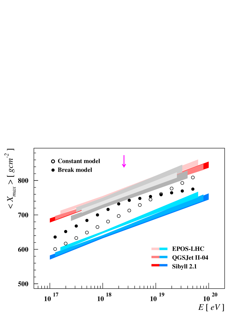
Figure 1: Average values of the depth of shower maximum are shown as functions of primary energy. Circles are for the constant elongation rate (constant model). Black full points are for the break model with two different elongation rates as indicated by a magenta arrow. Bands with red (blue) shade show $\langle X_{\rm max}\rangle$ predictions of the superposition model for primary protons (iron nuclei) that we received using CONEX showers generated with primary energies around $1\,{\rm EeV}$ within the indicated models of hadronic interactions. Gray bands show $\langle x_{\rm max}\rangle(E)$ for protons that we chose in seeking for four–component solutions of the constant model (light middle band) and break model (two darker gray bands), see Sections 4.1 and  4.2.

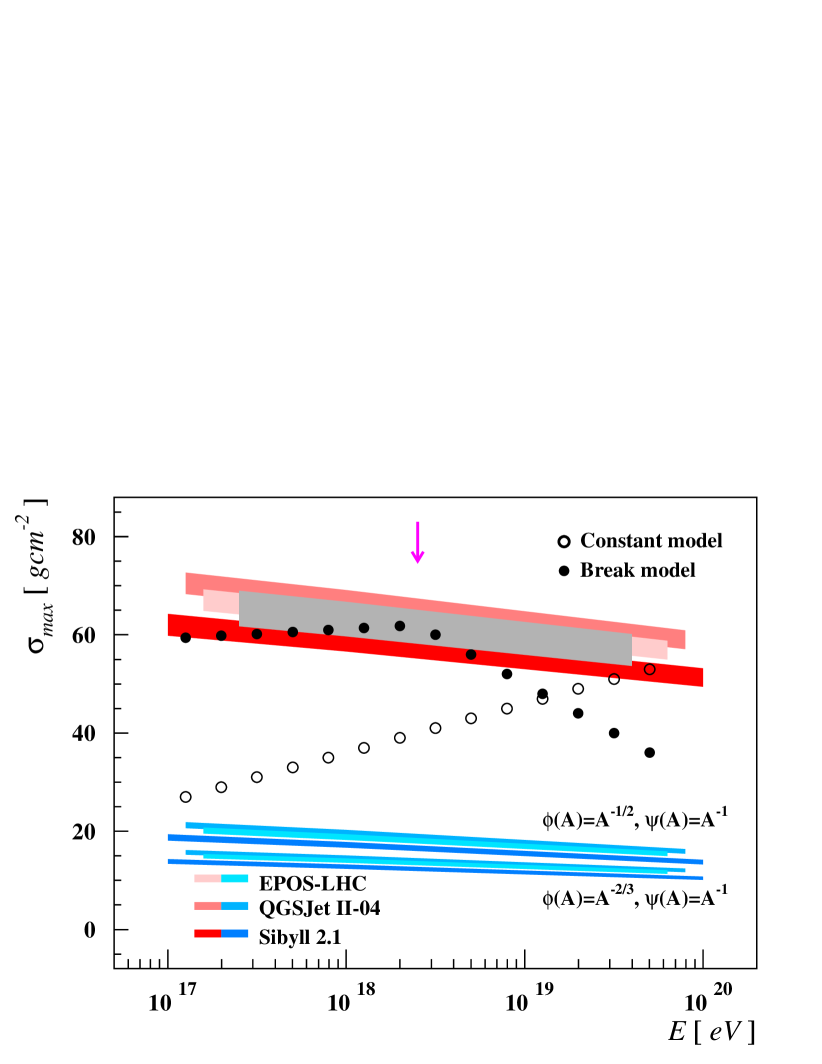
Figure 2: Standard deviations of the depth of shower maximum are shown as functions of primary energy. Circles are for the logarithmically increasing standard deviations (constant model). Black full points are for the break model with a break indicated by a magenta arrow. Bands with red (blue) shade are for $\sigma_{\rm max}$ predictions for primary protons (iron nuclei). They are based on the estimates of shower fluctuations given in A with parameters deduced from CONEX showers generated with primary energies around $1\,{\rm EeV}$ within the indicated models of hadronic interactions. Lower (upper) blue bands for iron nuclei are for the mass dependent terms $\phi(A)=A^{-\frac{2}{3}}(A^{-\frac{1}{2}})$ while $\psi(A)=A^{-1}$, see A. Our parametrization of the square root of the sum of shower variances for protons is shown by a gray band with $5\%$ uncertainties included.

The shower observables, $\langle X_{\rm max}\rangle$ and $\sigma^{2}_{\rm max}$, were decomposed using different sets of primary particles. Since it was not feasible to consider all the possible nuclei, we limited our analysis to primaries representing light, intermediate and heavy nuclei. We present results with primary protons ($A=1$), and helium ($A=4$), nitrogen ($A=14$) and iron ($A=56$) nuclei. This option is useful for examination of the impact of individual components in terms of reducing their number. Also other possibilities are briefly mentioned.

The obtained results depend on the quartet of shower parameters, namely, $C=\langle x_{\rm max}\rangle(E_{0})$, $D$, $\sigma_{\rm fr,0}^{2}=\sigma_{\rm fr}^{2}(A=1,E_{0})$ and $\sigma_{\rm sh,0}^{2}=\sigma_{\rm sh}^{2}(A=1,E_{0})$, and also on functions describing mass dependent fluctuations of the EAS development. Given the shower observables, $\langle X_{\rm max}\rangle(E)$ and $\sigma^{2}_{\rm max}(E)$, it turned out that only a certain set of the parameters $C$ and $D$ allows to find solutions to the partition problem in the whole energy range studied. The impact of other parameters that are associated with shower fluctuations was also examined.

With the aim of obtaining useful information from the data, we focus on how to exploit the potential of the partition concept. In this study, possible uncertainties of the $X_{\rm max}$ statistics and uncertainties of the energy scale are not taken into account. The estimates of their impact on resulting solutions can be obtained in repeated calculations with input data shifted according to these uncertainties. The ambiguities in resultant distributions with maximum entropy, as indicated below, occur herein just through unknown details of EAS physics. They are mainly associated with unknown though acceptable values of the parameters $C$ and $D$ that determine properties of proton showers. When presenting our final results of the mass decomposition, the values of these parameters are kept near the ranges reported by the CR experiments considering the predictions of the models of hadronic interactions [8, 9].

In a preliminary analysis, we successfully applied the maximum entropy method to a number of hypothetical examples. In order to test this method we assumed different mixtures of four or more primary species. With each chosen set of primary fractions we generated the two lowest order $X_{\rm max}$ moments within the shower model with fixed parameters. Then, these data were decomposed back to individual components, as dictated by the partition method. All the selected input tasks dominated by very different types of primaries were positively identified when seeking solutions with four or more components. Also predetermined fractions of the lightest species were reproduced with sufficient accuracy. They did not change much when extra particles were added. In complex ambiguous cases, it turned out, as expected, that the method of maximum entropy prefers to attribute similar occupation probabilities to heavier primaries.

In the following, we present results of two more sophisticated examples which provided us with nontrivial solutions. A special attention was paid to cases with the energy evolution of shower characteristics reminiscent of their measured dependencies. In a constant (elongation rate) model, we assumed that the average depth of shower maximum and its standard deviation increase linearly with the logarithm of the primary energy. In the second example, in a break model, we modeled breaks in the energy dependence of these statistics. In both cases, the two lowest order $X_{\rm max}$ moments were given for energies ranging from ${\rm Log}(E/\,{\rm eV})=17.1$ to $19.7$ for $14$ values in steps of $0.2$. The input dependencies are visualized in Figs.1 and 2. In these figures, we also show the $\langle X_{\rm max}\rangle=\langle X_{\rm max}\rangle(E)$ predictions of the superposition model and the estimates of shower fluctuations, $\sigma_{\rm max}=\sigma_{\rm max}(E)$, derived with the approach of A. All these estimates were obtained with the parameters calculated within the indicated models of hadronic interactions, see Section 2.

4.1 Constant model

The motivation for this example was to show what kind of solution is achieved when the input sample moments indicate that the transition from a predominantly heavy to light composition takes place. We used the average depth of shower maximum with a constant elongation rate. We assumed that the standard deviation of shower maximum grows logarithmically with the primary energy. Both these shower statistics, $\langle X_{\rm max}\rangle(E)$ and $\sigma_{\rm max}(E)$, displayed by circles in Figs.1 and 2, were chosen in such a way that

$$\frac{\langle X_{\rm max}\rangle(E)-X_{0}}{D_{0}}=\frac{\sigma_{\rm max}(E)-\sigma_{0}}{s_{0}}={\rm Log}\left(\frac{E}{E_{0}}\right).$$ (10)

Here we used $X_{0}=673~{}\,{\rm gcm^{-2}}$ and $\sigma_{0}=36~{}\,{\rm gcm^{-2}}$ for the $X_{\rm max}$ statistics given at a reference energy of $E_{0}=1~{}\,{\rm EeV}$. The remaining parameters were $D_{0}=80~{}\,{\rm gcm^{-2}}$ and $s_{0}=10~{}\,{\rm gcm^{-2}}$.

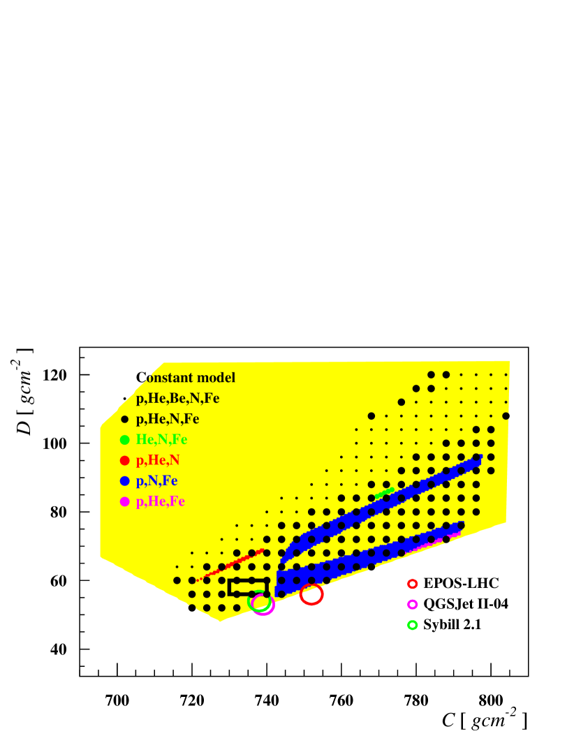
Figure 3: $C$–$D$ domains for acceptable solutions of the constant model. Yellow area is given by inequalities (5). A domain for acceptable four–component (p,He,N,Fe) solutions to the maximum entropy problem, shown by large black points in steps of $4~{}\,{\rm gcm^{-2}}$, is enlarged by five–component (p,He,N,Be,Fe) solutions as indicated by small black points. Green, red, blue and magenta areas show $C$–$D$ domains for (He,N,Fe), (p,He,N), (p,N,Fe) and (p,He,Fe) solutions, respectively. Colored circles indicate the $C$–$D$ ranges for the EPOS-LHC (red), QGSJet II-04 (blue) and Sibyll 2.1 (green) model as obtained by fitting their $\langle X_{\rm max}\rangle$ values for H, He, N and Fe primary nuclei to Eq.(1). In the partition analysis, we used parameters located inside a black rectangle.

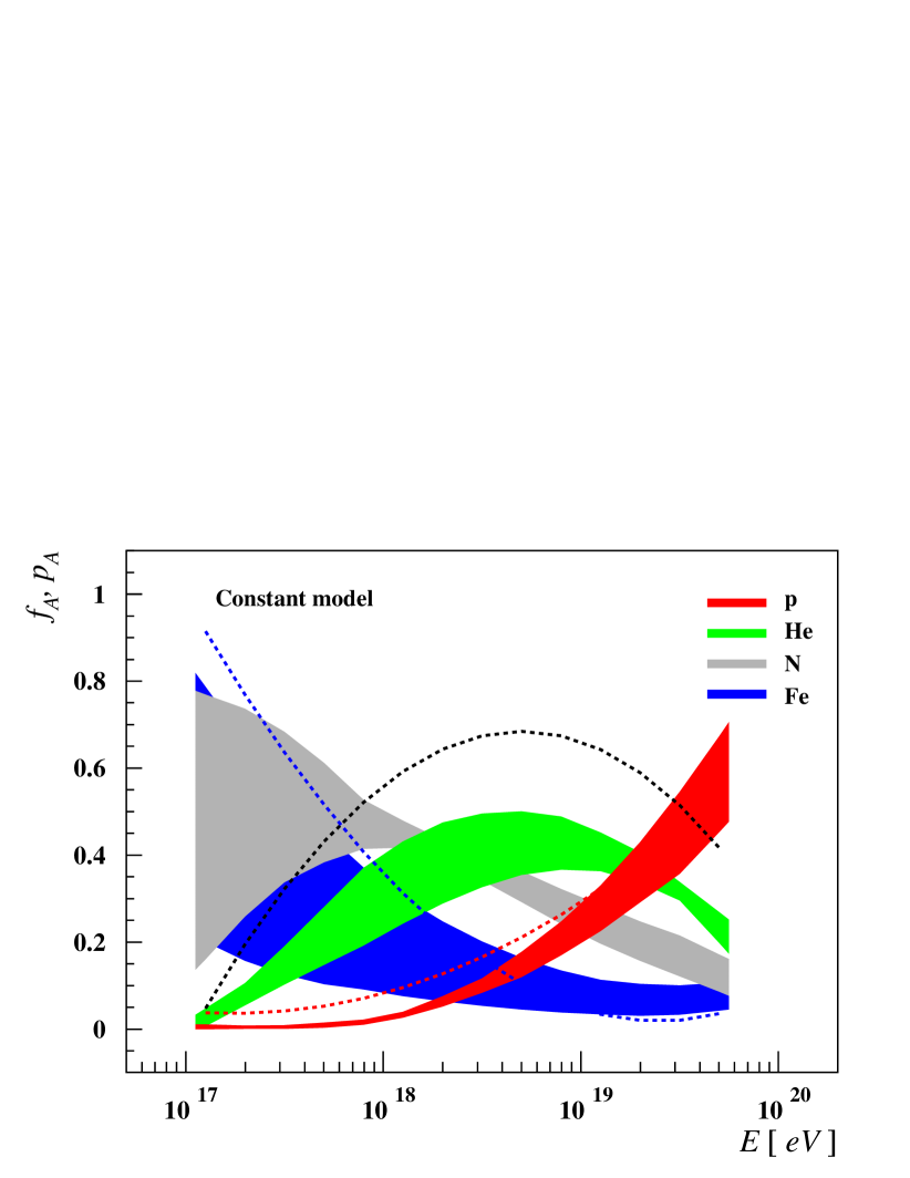
Figure 4: Probabilities of (p,He,N,Fe) partition of the constant model are depicted as functions of primary energy. Red, green, gray and blue bands are for proton, helium, nitrogen and iron components, respectively. Their widths correspond to the freedom in choosing the model parameters $C$ and $D$. We used $C\in\langle 730,740\rangle\,{\rm gcm^{-2}}$ and $D\in\langle 56,60\rangle\,{\rm gcm^{-2}}$, see the black rectangle in Fig.3. Dashed color curves show (p,N,Fe) solution with $C=744\,{\rm gcm^{-2}}$ and $D=56\,{\rm gcm^{-2}}$.

In the first step, we solved the partition problem numerically with four or more components leaving the two parameters $C$ and $D$ free. For the shower fluctuations, we used parametrizations that are described in A, see Eqs.(13) and (14). Their parameters were kept constant, i.e. we used $\sigma_{\rm fr,0}=46\,{\rm gcm^{-2}}$ and $\sigma_{\rm sh,0}=38\,{\rm gcm^{-2}}$. For the mass dependent terms we adopted $\phi(A)=A^{-\frac{2}{3}}$ and $\psi(A)=A^{-1}$. We assumed that the variance of the first interaction is energy dependent as given in Eq.(13) where we set $\xi(E)=1-0.2~{}{\rm Log}(E/\,{\rm EeV})$.

Using these assumptions, we searched for domains in the $C$–$D$ plane with acceptable maximum entropy solutions. By this we mean that the input information is compatible with the shower model, i.e. the accuracy with which the set of constraints written in Eqs.(8) and (9) is satisfied in the whole considered energy range is better than $10^{-2}$.

Resultant $C$–$D$ domains are visualized in Fig.3. The yellow area, the part of which is shown in the figure, is constructed using inequalities (5) for the primary masses $1\leq A\leq 56$. Large black points in Fig.3, shown in steps of $4~{}\,{\rm gcm^{-2}}$, represent possible values of the parameters $C$ and $D$ for which four–component solutions were determined. Acceptable solutions with five components enlarge the space for the model parameters as indicated by small black points. We also show the ranges of the parameters $C$ and $D$ that follow from our fits of $\langle X_{\rm max}\rangle$ values to the superposition ansatz while using CONEX showers initiated by H, He, N and Fe primary nuclei within the indicated generators of hadronic interactions.

The trend for the parameters $C$ and $D$ is well visible. The acceptable four– or more–component solubility of the maximum entropy problem demands larger proton elongation rates, $D>50\,{\rm gcm^{-2}}$. Increasing the parameter $C$, the acceptable values for the proton elongation rate should be even larger. Adding one or more light components ($A=6-12$) to the four–component conjecture, the size of the acceptable region is further enlarged towards larger values of the proton elongation rate $D$ (small black points in Fig.3). With the increasing number of intermediate or heavier components ($A=16-54$), the $C$–$D$ regions for acceptable solutions with five or more components remain within the boundaries given by the domain for four–component solutions. In this case we conclude that the most important part of the input information is exhausted by four–component solutions.

Different values for the parameters $C$ and $D$ of existing three–component solutions of the system of Eqs.(3) and (4) are also indicated in Fig.3. These solutions exist only in the well separated $C$–$D$ regions. The most of such deterministic solutions is for the triad of primary particles (p,N,Fe), see the blue regions in Fig.3.

In the second step, we made an attempt to derive the energy evolution of partition probabilities for primary particles causing showers with given $X_{\rm max}$ statistics. We performed the partition analysis with a selected set of the parameters $C$ and $D$ that yield acceptable solutions to the maximum entropy problem. Having no other supporting facts we simply explored a certain $C$–$D$ region in which the two constraints written in Eqs.(8) and (9) are satisfactorily fulfilled. We focused on small values of the proton elongation rate $D$, as observed in CR experiments (see Section 2), and those solutions that do not contradict the predictions of the current models of hadronic interactions (see also Figs.1 and 2). In making this decision, the whole set of energy dependent constraints was considered. In particular, the parameters were chosen in the vicinity of the predictions of the QGSJet II-04 and Sibyll 2.1 models, as indicated in Fig.3.

A four–component result of the partition analysis that was obtained with the parameters indicated in the figure caption (see black rectangle in Fig.3 and also middle light gray band in Fig.1) is plotted in Fig.4. In this figure, the decomposition probabilities of primary particles derived from the given $X_{\rm max}$ statistics are shown as functions of the primary energy. The widths of the colored bands correspond to aforementioned freedom in the parameters $C$ and $D$. We verified that these bands also comprise four–component solutions with the values of the parameters of shower fluctuations shifted by $\pm 5\%$ (see Fig.2) and with different mass dependent functions as described in A. For the sake of comparison, one selected three–component solution that does not include helium nuclei (blue region in Fig.3) is also shown in Fig.4.

For the sample mean and variance of the depth of shower maximum logarithmically growing with the primary energy, the transition from heavier to light primaries was identified in the resulting probability distributions of primary particles. A mixture of heavier primaries with very uncertain occupation probabilities together with negligible contributions of lighter species was obtained at the lowest primary energies. With the increasing energy, as both the $X_{\rm max}$ statistics grow, lighter primaries were found to be responsible for this kind of behavior, since the probability of finding them in a primary beam increases. The second lightest primaries (He or N nuclei) play a crucial role during the transition from shallow to deep showers accompanied by the increase of fluctuations in the depth of shower maximum. The partition method provides a solution in which a well established proton component dominates at the highest energies. We verified that the course of the transition from heavier to light primaries, as found in the four–component solutions, remains nearly unchanged with the increasing number of primaries included.

4.2 Break model

We also analyzed a set of shower statistics that resembles the experimental data that have been collected by the fluorescence detector of the Pierre Auger observatory [1, 2, 3, 4]. We prepared the input data, $\langle X_{\rm max}\rangle(E)$ and $\sigma_{\rm max}(E)$, with breaks as depicted in Figs.1 and 2 by black full points. For the energy dependence of the average depth of shower maximum we chose the elongation rate of $D_{0}=80~{}\,{\rm gcm^{-2}}$ for the primary energies below ${\rm Log}(E/\,{\rm eV})=18.4$ and $D_{0}^{\prime}=27~{}\,{\rm gcm^{-2}}$ above this energy with the parameter $X_{0}=708~{}\,{\rm gcm^{-2}}$, see Eq.(10). For the energy dependence of the standard deviation of the depth of shower maximum (see Eq.(10)), we took the value $s_{0}=2~{}\,{\rm gcm^{-2}}$ for ${\rm Log}(E/\,{\rm eV})<18.4$, $s_{0}^{\prime}=-20~{}\,{\rm gcm^{-2}}$ otherwise, and $\sigma_{0}=61.2~{}\,{\rm gcm^{-2}}$.

First, we were interested in permissible values for the parameters of the proton showers, $C$ and $D$. Assuming four or more primary species are responsible for the energy dependent $X_{\rm max}$ moments, we examined different types of maximum entropy solutions. We used the same parametrization for the shower fluctuations as given in the previous example in Section 4.1.

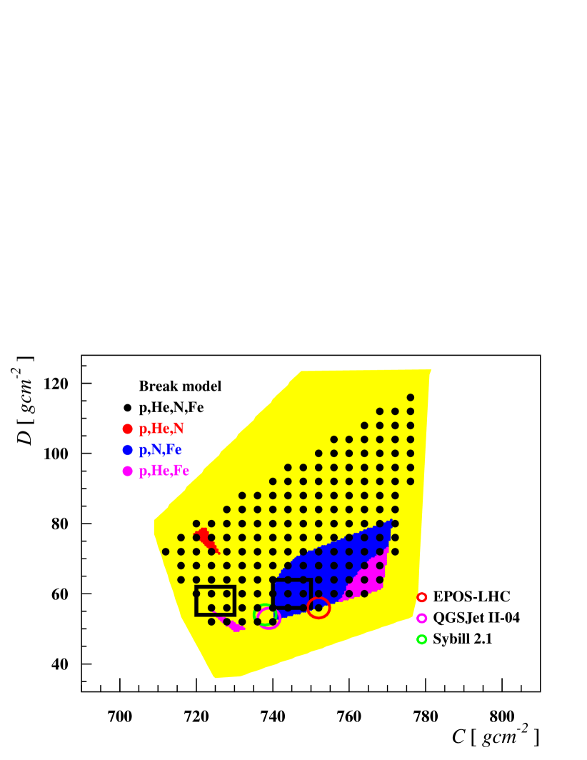
Figure 5: $C$–$D$ domains for acceptable solutions of the break model. Yellow area is given by inequalities (5). Large black points, shown in steps of $4~{}\,{\rm gcm^{-2}}$, represent acceptable four–component solutions to the maximum entropy problem for the (p,He,N,Fe) primary beam. Red, blue and magenta areas show $C$–$D$ regions for (p,He,N), (p,N,Fe) and (p,He,Fe) solutions, respectively. The region of (p,N,Fe) solutions (shown in blue) is partially overlapped with the (p,He,Fe) region (drawn in magenta). Colored circles indicate the ranges of $C$ and $D$ for the EPOS-LHC (red), QGSJet II-04 (blue) and Sibyll 2.1 (green) model. In the examples shown in Figs.6 and 7, we used parameters lying inside the left and right black rectangle, respectively.

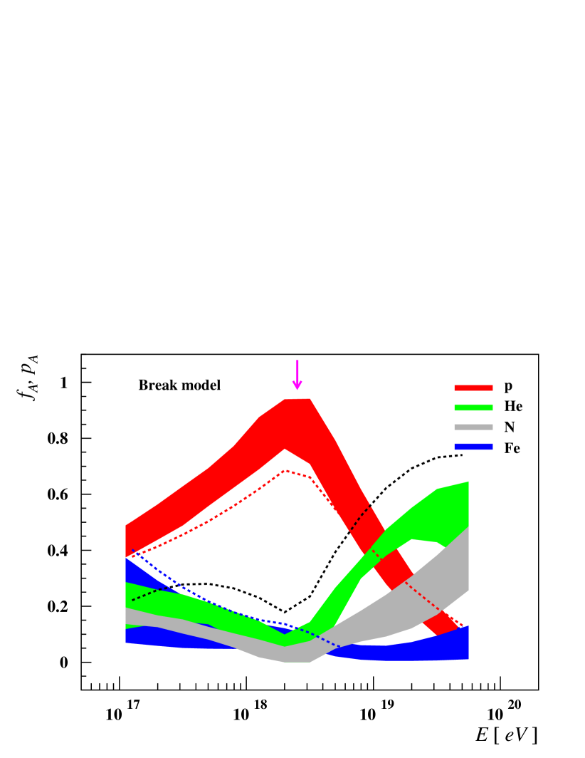
Figure 6: Probabilities of (p,He,N,Fe) partition for the break model are depicted as functions of primary energy, see also caption to Fig.4. We used $C\in\langle 720,730\rangle\,{\rm gcm^{-2}}$ and $D\in\langle 54,62\rangle\,{\rm gcm^{-2}}$, see the left black rectangle in Fig.5. Dashed color curves show (p,N,Fe) solutions with $C=740\,{\rm gcm^{-2}}$ and $D=56\,{\rm gcm^{-2}}$.

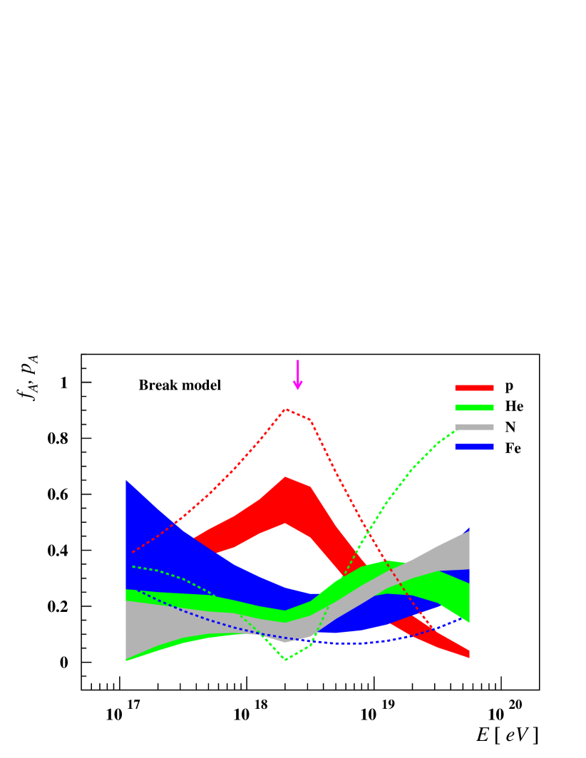
Figure 7: Probabilities of (p,He,N,Fe) partition for the break model are depicted as functions of primary energy, see also caption to Fig.4. They were obtained with the parameters $C\in\langle 740,750\rangle\,{\rm gcm^{-2}}$ and $D\in\langle 56,64\rangle\,{\rm gcm^{-2}}$, see the right black rectangle in Fig.5. Dashed color curves show (p,He,Fe) solutions with $C=724\,{\rm gcm^{-2}}$ and $D=56\,{\rm gcm^{-2}}$.

Resultant domains of the parameters $C$ and $D$ that provide solutions in the whole energy range are shown in Fig.5. The yellow area, the part of which is depicted in the figure, corresponds to inequalities (5) for the masses $1\leq A\leq 56$. The model parameters of acceptable four–component solutions were determined in steps of $4~{}\,{\rm gcm^{-2}}$, as shown by large black points. With further increase of the number of primary components above four, the $C$–$D$ regions giving acceptable solutions stay within the boundaries of the four–component $C$–$D$ domain. Also, the $C$–$D$ regions for different types of three–component solutions are indicated in Fig.5. Colored circles show the ranges of relevant parameters estimated with the help of the models of hadronic interactions.

In this example, we learned that the input information on the energy evolution of the two lowest order $X_{\rm max}$ moments is well described by four–component solutions to the maximum entropy problem. A range of the model parameters $C$ and $D$ providing these solutions is not in conflict with their current estimations [8, 9].

In order that three–component solutions exist for all considered energies, the proton elongation rate $D>50\,{\rm gcm^{-2}}$ and even larger value ($D>70\,{\rm gcm^{-2}}$) is required if three–component solutions without iron nuclei are constructed, see the red region in Fig.5. We found that the proton component cannot be missed in any case. There is a large domain of the parameters $C$ and $D$ providing three–component solutions without primary helium, see the blue region in Fig.5 that is partially overlapped with the $C$–$D$ domain of the (p,He,Fe) solutions shown in magenta.

Finally, we were concerned with the probability distributions of primary species as they can be derived in the decomposition analysis using the input information about the two lowest order $X_{\rm max}$ moments. We carried out the partition analysis with the parameters $C$ and $D$ that yield acceptable solutions to the maximum entropy problem. In order to illustrate the impact of the parameter selection, we examined in this case two different $C$–$D$ domains. We chose one set of parameters with small reference values of the mean depth of shower maximum for protons and the second set located near the predictions of the models of hadronic interactions, see two black rectangles in Fig.5.

A resultant four–component partition is shown as a function of the primary energy in Fig.6. It was obtained with the parameters indicated in the figure caption (see left black rectangle in Fig.3 and also lower dark gray band in Fig.1). Also a three–component partition that does not account for a fraction of helium (blue region in Fig.5) is presented in Fig.6. In Fig.7, a four–component partition to the maximum entropy problem obtained for a different set of the model parameters (see right black rectangle in Fig.3 and also upper dark gray band in Fig.1) is shown together with another three–component solution to Eqs.(3) and (4), in this case without nitrogen nuclei. The breaks modeled in the energy dependencies of the two $X_{\rm max}$ statistics are well visible in the partition probabilities of all these solutions.

Within the proposed method, we succeeded in the description of energy dependencies of the two lowest order $X_{\rm max}$ moments. The resultant evolution of the probability distribution of particles in the primary beam can be interpreted as follows. Apart from primary protons, second lightest primaries (He or N nuclei) were found to play an important role in the presented decomposition. The probability of the proton presence in the primary beam initially grows and then declines rapidly with the primary energy once it reaches its maximum value near the modeled break point at about ${\rm Log}(E/\,{\rm eV})=18.3$. Around this energy the remaining components are very likely to be drastically reduced. The proton dominance near the break point is diminished with the increasing value of the parameter $C$, while the role of the heaviest component (Fe nuclei) grows, compare Fig.6 with Fig.7. After the break point, the modeled transition from shallow to deep showers with a fall of fluctuations in the depth of shower maximum does not demand any substantial proton component. Instead, particles with intermediate masses or a complex mixture of intermediate and heavier nuclei were found to take over the main role. Adding one or more primary species, the typical features of this partition are preserved.

5 Conclusions

We used the well–reasoned method based on the maximum entropy principle to derive the partition of primary cosmic ray particles from the characteristics of the longitudinal development of extensive air showers that they initiated. A set of the first and second order $X_{\rm max}$ moments is used as the input data. The proposed approach combines the superposition ansatz and multiplication characteristics of air showers. As input parameters, the method needs the values of the mean depth of shower maximum for protons and of the elongation rate for protons, both at a chosen reference energy. The mass dependent terms associated with shower fluctuations, as inferred from experimental data, were proved to be applicable in the search for the primary mass composition.

We showed that simple assumptions about the properties of extensive air showers make the partition analysis suitable for exploring energy dependent changes in the composition of the primary beam of cosmic particles. In particular, we presented solutions to the partition problem for two hypothetical sets of the two lowest order $X_{\rm max}$ moments. It was shown that these data can be satisfactorily described by assuming that four groups of primary species are present in the primary beam. The partition method allowed us to partially reduce the parameter space within the model adopted for the shower development. With a set of parameters selected in agreement with experiments and model predictions we were able to assess specific solutions. While the role of the lightest primaries is indisputable, heavier particles were identified with more uncertainty. Our analysis indicates that primaries of intermediate masses are required when searching for reasonable solutions.

The proposed partition scheme constitutes a very simple way to extract undistorted information about the decomposition of the primary cosmic rays into individual species from the measured data. It relies on well known statistical arguments which delivers a special interpretation to results. Deduced in the maximum entropy method, the obtained partitions and subsequent conclusions have probabilistic nature by definition. In the analysis of shower observables, the resultant probability distributions of primary particles are least affected with regard to missing information, while respecting our knowledge of shower physics inserted into the calculations. In this sense, the selective ability of maximum entropy may help in the classification of available models of hadronic interactions.

Appendix A Shower variances

In our method, the mean depth of shower maximum for primary protons with an energy $E$ is assumed to be [8]

$$\langle x_{\rm max}\rangle(E)\approx\lambda(E)+X~{}\ln\left(\frac{\kappa E}{2M\epsilon}\right),$$ (11)

where $\lambda=\lambda(E)$ is the mean interaction length for inelastic $p$–air collisions, $X\approx 37~{}\,{\rm gcm^{-2}}$ is the radiation length in air and $\epsilon\approx 84~{}\,{\rm MeV}$ denotes the critical energy in air. Both the elasticity of the first interaction, $\kappa=\kappa(E)$, and its multiplicity, $M=M(E)$, are energy dependent. The relationship written in Eq.(11) is well documented within the Heitler model extended to hadronic showers [8].

For the variance of the depth of the first interaction we employed the measured $p$–air cross section at a center of mass energy of $\sqrt{s}=57~{}\,{\rm TeV}$ [41]. Relying upon a smooth extrapolation from accelerator measurements, and in agreement with model predictions, we used for its parametrization

$$\Sigma_{\rm p-Air}\approx\left[500+50~{}{\rm Log}(E/\,{\rm EeV})\right]\,{\rm mb}.$$ (12)

Within a naive model, the variance of the depth of the first interaction of a primary nucleus with $A$ nucleons colliding with the air target is then approximately

$$\sigma_{\rm fr}^{2}=\sigma_{\rm fr}^{2}(A,E)\approx\phi(A)\xi(E)\sigma_{\rm fr,0}^{2},$$ (13)

where $\phi=\phi(A)$ denotes a mass dependent term and $\xi=\xi(E)$ is a general dependence of the variance on the primary energy. A value of the square root of the variance of the depth of the first interaction caused by primary protons at a reference energy of $E_{0}=1~{}\,{\rm EeV}$, $\sigma_{\rm fr,0}=\lambda(E_{0})\approx 46~{}\,{\rm gcm^{-2}}$, as well as a constant in the energy dependent function $\xi(E)\approx 1-0.2~{}{\rm Log}(E/\,{\rm EeV})$, were deduced from the parametrization given in Eq.(12).

The mass dependent term in Eq.(13), $\phi=\phi(A)$, accounts for the details of the first interaction given by individual nucleon–nucleon interactions and subsequent nuclear fragmentation [8]. Averaging over all available numbers of simultaneously interacting nucleons accompanied by the remaining number of free spectator nucleons, we obtained for the variance of the depth of the first interaction $\phi_{1}(A)=\frac{1}{3}+\frac{1}{A}-\frac{1}{3A^{2}}>A^{-\frac{1}{2}}$. Since $\phi_{0}(A)=A^{-1}$ is expected for $A$ free nucleons, we chose the mass dependent function $\phi(A)=A^{-\alpha}$ with a constant index $\alpha=\frac{2}{3}$, i.e. $\phi_{0}<\phi<\phi_{1}$ for any $A$. We also examined values of $\alpha$ ranging from $\frac{1}{3}$ up to $1$. These values yielded slightly different results, with deviations below uncertainties that are due to the ambiguity of other shower parameters.

The variance of the depth of shower maximum in the subsequent shower development is given by

$$\sigma_{\rm sh}^{2}=\sigma_{\rm sh}^{2}(A,E)\approx\psi(A)\sigma_{\rm sh,0}^{2},$$ (14)

where the function $\psi=\psi(A)$ is responsible for the mass effects. The parameter $\sigma_{\rm sh,0}\approx 38~{}\,{\rm gcm^{-2}}$, the square root of the shower variance for primary protons, was estimated from the standard deviation of the depth of shower maximum $\sigma_{\rm max}\approx 60~{}\,{\rm gcm^{-2}}$ measured at about $1~{}\,{\rm EeV}$ [1, 2, 3, 4], when mostly primary protons are assumed to cause such showers. Experimentally, the standard deviation of the depth of shower maximum declines with the increasing energy showing that heavier primaries with a narrower mass distribution are responsible [4, 8, 9, 12]. Hence, the square root of the shower variance for primary protons has a lower bound somewhere below the indicated value when an unknown primary composition is observed at the reference energy.

The mass dependent term of the shower variance, $\psi=\psi(A)$, is given by fluctuations in multiplicity $M$ and elasticity $\kappa$ of the first (or main) interaction. Assuming a simple concept introduced in Eq.(11), the corresponding shower variance caused by primary protons is $\sigma_{\rm sh,0}^{2}=\sigma_{\rm M,0}^{2}+\sigma_{\rm\kappa,0}^{2}$ where

$$\sigma_{\rm M,0}^{2}\approx X^{2}\frac{\sigma_{\rm M}^{2}}{M^{2}},\qquad\qquad\sigma_{\rm\kappa,0}^{2}\approx X^{2}\frac{\sigma_{\rm\kappa}^{2}}{\kappa^{2}}.$$ (15)

Here $\sigma_{\rm M}^{2}$ and $\sigma_{\rm\kappa}^{2}$ denote, respectively, the variances in multiplicity and elasticity associated with the main interaction. In a naive superposition model [8], the variance of the total multiplicity of $k$ out of $A$ nucleons participating in the main interaction with a multiplicity $\overline{M}$ averaged over all projectile nucleons is given by $\sigma^{2}(k\overline{M})=k^{2}A^{-1}\sigma_{\rm M}^{2}$. In a similar manner, one gets $\sigma^{2}(\overline{\kappa})=A^{-1}\sigma_{\rm\kappa}^{2}$ for an average elasticity $\overline{\kappa}$ taken over all projectile nucleons. Hence, we used $\psi(A)=A^{-1}$ in this approach.

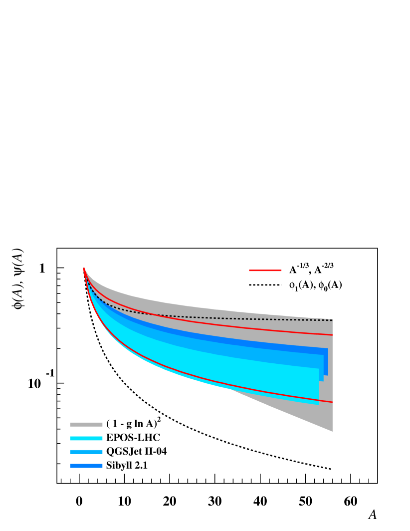
Figure 1: Parametrization of shower variances. Black dashed curves show, respectively, an average value for the $A$–dependent term of the variance of the depth of the first interaction with one cluster of nucleons, $\phi_{1}(A)$ (upper curve), or with free nucleons, $\phi_{0}(A)$ (lower curve). The mass dependent terms $\phi(A)=A^{-\frac{1}{3}}$ (upper curve) and $\phi(A)=A^{-\frac{2}{3}}$ (lower curve) are shown in red. Gray band is for the parametrization of the shower variances taken from Ref. [30]. Bands in blue shade represent our parametrizations obtained with CONEX showers using the EPOS-LHC, QGSJet II-04 and Sibyll 2.1 models.

In order to get a better overview of the problem of the shower fluctuations, we examined the logarithmic parametrization of the total shower variance as suggested in Ref. [30]. Specifically, we took $\phi(A)=\psi(A)\approx\left(1-g\ln A\right)^{2}$, where the parameter $g=0.15\pm 0.05$ [30]. The energy dependence for the variance of the depth of the first interaction was included, see Eq.(13). Since air shower simulations are known to predict larger shower variances for heavy primaries than expected from naive considerations, we also examined less steep dependencies on the primary mass, namely, $\phi(A)=\psi(A)=A^{-\frac{1}{2}}$. This choice was supported by overall shower fluctuations that were derived using a set of CONEX showers [40] generated with energies around $1\,{\rm EeV}$ for H, He, N and Fe primary nuclei within the EPOS-LHC [36, 37], QGSJet II-04 [38] and Sibyll 2.1 [39] models. In these simulations, we received mass dependent terms $\phi(A)=\psi(A)\approx A^{-\alpha}$ where $\alpha\approx 0.58,0.49$ and $0.46$, respectively, with uncertainties about $15\%$. In summary, dealing with each of the above assumptions, we obtained similar results.

Different mass dependent functions used for the shower variances are depicted in Fig.1. While these variances are little dependent on the primary mass for $A>20$, lighter nuclei ($A<10$) give very different contributions. Based on this approximation that pursue the current knowledge of the shower physics, medium and heavier nuclei can hardly be distinguished on the basis of shower fluctuations.

Appendix B Maximum entropy formalism

Let us assume that the quantity $A$ is capable to take $n$ discrete values $A=1,\dots,n$. Corresponding probabilities $p_{\rm A}$ are not known, however. Only a set of $r$ expectation values of the functions $F_{i}(A)$, $i=1,\dots,r$, $r<n$, is measured. For setting up a probability distribution which satisfies the given data, the least biased estimate possible on the basis of partial knowledge is used. The underlying information–theoretic principle, known as the maximum entropy principle, was originally introduced in the context of statistical physics [32]. For its use in statistics see e.g. Ref. [34].

The overriding principle of this procedure matches an intuition of how maximally unbiased estimates should be achieved in the absence of detailed information about investigated phenomena. Here, Shannon entropy [32, 35]

$$S=-k\sum\limits_{A=1}^{n}p_{\rm A}\ln p_{\rm A},$$ (16)

where $k$ is a positive constant, is used as an information measure of the amount of uncertainty in the probability distribution $p_{\rm A}$ of the quantity $A$. This distribution is determined as the one that maximizes entropy $S$ in Eq.(16) subject to $r$ constraints, $F_{i}(A)$, $i=1,\dots,r$, given their averages that represent whatever experimental information one has, i.e.

$$\langle F_{i}\rangle=\sum\limits_{A=1}^{n}p_{\rm A}F_{i}(A),\quad i=1,\dots,r,$$ (17)

subject to the normalization condition $\sum\limits_{A=1}^{n}p_{\rm A}=1$. Then, the resultant distribution describes what we know about the quantity $A$ from experiment without assuming anything else about the data [32].

In making inferences on the basis of partial information, the maximum entropy probability distribution that maximizes Shannon entropy in Eq.(16) subject to the experimental constraints written in Eq.(17) is given by [32, 35]

$$p_{\rm A}=Z^{-1}e^{-\left[\lambda_{1}F_{1}(A)+\dots+\lambda_{r}F_{r}(A)\right]},$$ (18)

with the partition function written

$$Z(\lambda_{1},\dots,\lambda_{r})=\sum\limits_{A=1}^{n}e^{-\left[\lambda_{1}F_{1}(A)+\dots+\lambda_{r}F_{r}(A)\right]},$$ (19)

and with Lagrangian multipliers $\lambda_{i}$, $i=1,\dots,r$, to be determined. Then, based on Shannon’s information measure, the resultant probability distribution $p_{\rm A}$ of the quantity $A$ obtained in this process is spread out as widely as possible without contradicting the available experimental information represented by the average values of the constraints. For further details see e.g. Ref. [35] and references therein.

Acknowledgment: We would like to acknowledge many useful discussions with our colleagues of the Pierre Auger Collaboration. We thank to two unknown reviewers that help us with the presentation of this study. This work was supported by the Czech Science Foundation grant 14-17501S. The research of J.N. was supported by the Czech Science Foundation under project GACR P103/12/G084.

References

- [1] J.Abraham et al., Phys.Rev.Lett. 104 (2010) 091101.
- [2] P.Facal and Pierre Auger Collaboration, Proc. 32th International Cosmic Ray Conference, Beijing, Vol.2, 2011, p.105.
- [3] V.de Souza for the Pierre Auger Collaboration, Proc. 33th International Cosmic Ray Conference, Rio de Janeiro, arXiv:1307.5059.
- [4] A.Aab et al., Phys.Rev. D 90 (2014) 122005.
- [5] R.U.Abbasi et al., Phys.Rev.Lett. 104 (2010) 161101.
- [6] R.U.Abbasi et al., Astroparticle Physics 64 (2015) 49.
- [7] E.G.Berezhko, S.P.Knurenko, L.T.Ksenofontov, Astroparticle Physics 36 (2012) 31.
- [8] K.–H.Kampert, M.Unger, Astroparticle Physics 35 (2012) 660.
- [9] E.Barcikowski et al.for the Pierre Auger, Telescope Array, Yakutsk Collaborations, EPJ Web of Conferences 53 (2013) 01006.
- [10] P.Abreu, et al., JCAP 02 (2013) 026.
- [11] E.J.Ahn for the Pierre Auger Collaboration, Proc. 33th International Cosmic Ray Conference, Rio de Janeiro, arXiv:1307.5059.
- [12] A.Aab et al., Phys.Rev. D 90 (2014) 122006.
- [13] M.De Domenico, M.Settimo, S.Riggi, E.Bertin, JCAP 07 (2013) 050.
- [14] S.Riggi, S.Ingrassia, Astroparticle Physics 48 (2013) 86.
- [15] D.Garcí–Gámez for the Pierre Auger Collaboration, Proc. 33th International Cosmic Ray Conference, Rio de Janeiro, arXiv:1307.5059.
- [16] I.Valiño for the Pierre Auger Collaboration, Proc. 33th International Cosmic Ray Conference, Rio de Janeiro, arXiv:1307.5059.
- [17] B.Kégl for the Pierre Auger Collaboration, Proc. 33th International Cosmic Ray Conference, Rio de Janeiro, arXiv:1307.5059.
- [18] G.R.Farrar for the Pierre Auger Collaboration, Proc. 33th International Cosmic Ray Conference, Rio de Janeiro, arXiv:1307.5059.
- [19] P.Younk, M.Risse, Astroparticle Physics 35 (2012) 807.
- [20] A.Aab et al, Phys.Rev. D 90 (2014) 012012.
- [21] A.Aab et al, Phys.Rev. D 91 (2015) 032003.
- [22] M.Ambrosio, et al., Astroparticle Physics 24 (2005) 355.
- [23] S.Riggi, et al., Nuclear Instruments and Methods in Physics Research A 707 (2013) 9.
- [24] P.Abreu et al, Phys.Rev. D 84 (2011) 122005.
- [25] M.Lemoine, E.Waxman, JCAP 11 (2009) 009.
- [26] P.Abreu, et al., JCAP 06 (2011) 022.
- [27] A.M.Taylor, M.Ahlers, F.A.Aharonian, Phys.Rev. D 84 (2012) 205007.
- [28] R.Y.Liu, A.M.Taylor, M.Lemoine, X.Y.Wang, E.Waxman, The Astrophysical Journal 776 (2013) 88.
- [29] A.M.Taylor, Astroparticle Physics 54 (2014) 48.
- [30] J.Linsley, rapporteur paper in Proc. 18th International Cosmic Ray Conference, Bangalore, India, 12 (1983) 135.
- [31] J.Linsley, Proc. 19th International Cosmic Ray Conference, San Diego, California, 6 (1985) 1.
- [32] E.T.Jaynes, Phys.Rev. 106 (1957) 620.
- [33] E.T.Jaynes, Phys.Rev. 108 (1957) 171.
- [34] R.C.Rao, Linear Statistical Inference and Its Applications, John Willey & Sons, 1973.
- [35] S.Pressé, et al., Rev.Mod.Phys. 85 (2013) 1115.
- [36] K.Werner, F.M.Liu and T.Pierog, Phys.Rev. C74 (2006) 044902.
- [37] T.Pierog and K.Werner, Nucl.Phys. (Proc.Suppl.) 196 (2009) 102.
- [38] S.S.Ostapchenko, Phys.Rev. D83 (2011) 014018.
- [39] E.J.Ahn et al., Phys.Rev. D80 (2009) 094003.
- [40] T.Bergmann et al., Astroparticle Physics 26 (2007) 420.
- [41] P.Abreu, et al., Phys.Rev.Lett. 109 (2012) 062002.