Forecaster’s Dilemma: Extreme Events and Forecast Evaluation

Abstract

In public discussions of the quality of forecasts, attention typically focuses on the predictive performance in cases of extreme events. However, the restriction of conventional forecast evaluation methods to subsets of extreme observations has unexpected and undesired effects, and is bound to discredit skillful forecasts when the signal-to-noise ratio in the data generating process is low. Conditioning on outcomes is incompatible with the theoretical assumptions of established forecast evaluation methods, thereby confronting forecasters with what we refer to as the forecaster’s dilemma. For probabilistic forecasts, proper weighted scoring rules have been proposed as decision theoretically justifiable alternatives for forecast evaluation with an emphasis on extreme events. Using theoretical arguments, simulation experiments, and a real data study on probabilistic forecasts of U.S. inflation and gross domestic product (GDP) growth, we illustrate and discuss the forecaster’s dilemma along with potential remedies.

​​, ​​, ​​ and

Quod male consultum cecidit feliciter, Ancus,
Arguitur sapiens, quo modo stultus erat.
Quod prudenter erat provisum, si male vortat,
Ipse Cato (populo iudice) stultus erat.

John Owen, 1607

1 Introduction

Extreme events are inherent in natural or man-made systems and may pose significant societal challenges. The development of the theoretical foundations for the study of extreme events started in the middle of the last century and has received considerable interest in various applied domains, including but not limited to meteorology, climatology, hydrology, finance, and economics. Topical reviews can be found in the work of Gumbel (1958), Embrechts et al. (1997), Easterling et al. (2000), Coles (2001), Katz et al. (2002), Beirlant et al. (2004), and Albeverio et al. (2006), among others. Not surprisingly, accurate predictions of extreme events are of great importance and demand. In many situations distinct models and forecasts are available, thereby calling for a comparative assessment of their predictive performance with particular emphasis placed on extreme events.

In the public, forecast evaluation often only takes place once an extreme event has been observed, in particular, if forecasters have failed to predict an event with high economic or societal impact. Table 1 gives examples from newspapers, magazines, and broadcasting corporations that demonstrate the focus on extreme events in finance, economics, meteorology, and seismology. Striking examples include the international financial crisis of 2007/08 and the L’Aquila earthquake of 2009. After the financial crisis, much attention was paid to economists who had correctly predicted the crisis, and a superior predictive ability was attributed to them. In 2011, against the protest of many scientists around the world, a group of Italian seismologists was put on trial for not warning the public of the devastating L’Aquila earthquake of 2009 that caused 309 deaths (Hall, 2011). Six scientists and a government official were found guilty of involuntary manslaughter in October 2012 and sentenced to six years of prison each. In November 2015, the scientists were acquitted by the Supreme Court in Rome, whereas the sentence of the deputy head of Italy’s civil protection department, which had been reduced to two years in 2014, was upheld.

At first sight, the practice of selecting extreme observations, while discarding non-extreme ones, and to proceed using standard evaluation tools appears to be a natural approach. Intuitively, accurate predictions on the subset of extreme observations may suggest superior predictive ability. However, the restriction of the evaluation to subsets of the available observations has unwanted effects that may discredit even the most skillful forecast available (Denrell and Fang, 2010; Diks et al., 2011; Gneiting and Ranjan, 2011). In a nutshell, if forecast evaluation proceeds conditionally on a catastrophic event having been observed, always predicting calamity becomes a worthwhile strategy. Given that media attention tends to focus on extreme events, skillful forecasts are bound to fail in the public eye, and it becomes tempting to base decision-making on misguided inferential procedures. We refer to this critical issue as the forecaster’s dilemma.

Table 1: Media coverage illustrating the focus on extreme events in public discussions of the quality of forecasts. A version of the table with links to the sources is provided in an online supplement.

Year	Headline	Source
2008	Dr. Doom	The New York Times
2009	How did economists get it so wrong?	The New York Times
2009	He told us so	The Guardian
2010	Experts who predicted US economy crisis see recovery	Bloomberg
	in 2010
2010	An exclusive interview with Med Yones - The expert who	CEO Q Magazine
	predicted the financial crisis
2011	A seer on banks raises a furor on bonds	The New York Times
2013	Meredith Whitney redraws ‘map of prosperity’	USA Today
2007	Lessons learned from Great Storm	BBC
2011	Bad data failed to predict Nashville flood	NBC
2012	Bureau of Meteorology chief says super storm ‘just blew up	The Courier-Mail
	on the city’
2013	Weather Service faulted for Sandy storm surge warnings	NBC
2013	Weather Service updates criteria for hurricane warnings,	Washington Post
	after Sandy criticism
2015	National Weather Service head takes blame for forecast	NBC
	failures
2011	Italian scientists on trial over L’Aquila earthquake	CNN
2011	Scientists worry over ‘bizarre’ trial on earthquake	Scientific American
	prediction
2012	L’Aquila ruling: Should scientists stop giving advice?	BBC

To demonstrate the phenomenon, we let $\mathcal{N}(\mu,\sigma^{2})$ denote the normal distribution with mean $\mu$ and standard deviation $\sigma$ and consider the following simple experiment. Let the observation $Y$ satisfy

$$Y|\,\mu\sim\mathcal{N}(\mu,\sigma^{2})\quad\textnormal{where}\quad\mu\sim\mathcal{N}(0,1-\sigma^{2}).$$ (1.1)

Table 2 introduces forecasts for $Y$, showing both the predictive distribution, $F$, and the associated point forecast, $X$, which we take to be the respective median or mean. The perfect forecast has knowledge of $\mu$, while the unconditional forecast is the unconditional standard normal distribution of $Y$. The deliberately misguided extremist forecast shows a constant bias of $\frac{5}{2}$. As expected, the perfect forecast is preferred under both the mean absolute error (MAE) and the mean squared error (MSE). However, these results change completely if we restrict attention to the largest 5% of the observations, as shown in the last two columns of the table, where the misguided extremist forecast receives the lowest mean score.

In this simple example, we have considered point forecasts only, for which there is no obvious way to abate the forecaster’s dilemma by adapting existing forecast evaluation methods appropriately, such that particular emphasis can be put on extreme outcomes. Probabilistic forecasts in the form of predictive distributions provide a suitable alternative. Probabilistic forecasts have become popular over the past few decades, and in various key applications there has been a shift of paradigms from point forecasts to probabilistic forecasts, as reviewed by Tay and Wallis (2000), Timmermann (2000), Gneiting (2008), and Gneiting and Katzfuss (2014), among others. As we will see, the forecaster’s dilemma is not limited to point forecasts and occurs in the case of probabilistic forecasts as well. However, in the case of probabilistic forecasts extant methods of forecast evaluation can be adapted to place emphasis on extremes in decision theoretically coherent ways. In particular, it has been suggested that suitably weighted scoring rules allow for the comparative evaluation of probabilistic forecasts with emphasis on extreme events (Diks et al., 2011; Gneiting and Ranjan, 2011).

Table 2: Forecasts in the simulation study, where the observation $Y$ satisfies (1.1) with $\sigma^{2}=\frac{2}{3}$ being fixed. The mean absolute error (MAE) and mean squared error (MSE) for the point forecast $X$ are based on a sample of size 10 000; the restricted versions rMAE and rMSE are based on the subset of observations exceeding 1.64 only. The lowest value in each column is in bold.

Forecast	Predictive Distribution	$X$	MAE	MSE	rMAE	rMSE
Perfect	$\mathcal{N}(\mu,\sigma^{2})$	$\mu$	0.64	0.67	1.35	2.12
Unconditional	$\mathcal{N}(0,1)$	0	0.80	0.99	2.04	4.30
Extremist	$\mathcal{N}(\mu+\frac{5}{2},\sigma^{2})$	$\mu+\frac{5}{2}$	2.51	6.96	1.16	1.61

The remainder of the article is organized as follows. In Section 2 theoretical foundations on forecast evaluation and proper scoring rules are reviewed, serving to analyse and explain the forecaster’s dilemma along with potential remedies. In Section 3 this is followed up and illustrated in simulation experiments. Furthermore, we elucidate the role of the fundamental lemma of Neyman and Pearson, which suggests the superiority of tests of equal predictive performance that are based on the classical, unweighted logarithmic score. A case study on probabilistic forecasts of gross domestic product (GDP) growth and inflation for the United States is presented in Section 4. The paper closes with a discussion in Section 5.

2 Forecast evaluation and extreme events

We now review relevant theory that is then used to study and explain the forecaster’s dilemma.

2.1 The joint distribution framework for forecast evaluation

In a seminal paper on the evaluation of point forecasts, Murphy and Winkler (1987) argued that the assessment ought to be based on the joint distribution of the forecast, $X$, and the observation, $Y$, building on both the calibration-refinement factorization,

$$[X,Y]\,=\,[X]\>[Y|X],$$

and the likelihood-baserate factorization,

$$[X,Y]\,=\,[Y]\>[X|Y].$$

Gneiting and Ranjan (2013), Ehm et al. (2016), and Strähl and Ziegel (2015) extend and adapt this framework to include the case of potentially multiple probabilistic forecasts. The joint distribution of the probabilistic forecasts and the observation is then defined on a probability space $(\Omega,\mathcal{A},\mathbb{Q})$, where the elements of the sample space $\Omega$ can be identified with tuples

$$(F_{1},\ldots,F_{k},Y),$$

the distribution of which is specified by the probability measure $\mathbb{Q}$. The $\sigma$-algebra $\mathcal{A}$ can be understood as encoding the information available to forecasters. The predictive distributions $F_{1},\ldots,F_{k}$ are cumulative distribution function (CDF)-valued random quantities on the outcome space of the observation, $Y$. They are assumed to be measurable with respect to their corresponding information sets, which can be formalized as sub-$\sigma$-algebras $\mathcal{A}_{1},\ldots,\mathcal{A}_{k}\subseteq\mathcal{A}$. The predictive distribution $F_{i}$ is ideal relative to the information set $\mathcal{A}_{i}$ if $F_{i}=[Y|\mathcal{A}_{i}]$ almost surely. Thus, an ideal predictive distribution makes the best possible use of the information at hand. In the setting of eq. (1.1) and Table 2, the perfect forecast is ideal relative to knowledge of $\mu$, the unconditional forecast is ideal relative to the empty information set, and the extremist forecast fails to be ideal.

Considering the case of a single probabilistic forecast, $F$, the above factorizations have immediate analogues in this setting, namely, the calibration-refinement factorization

$$[F,Y]\,=\,[F]\>[Y|F]$$ (2.1)

and the likelihood-baserate factorization

$$[F,Y]\,=\,[Y]\>[F|Y].$$ (2.2)

The components of the calibration-refinement factorization (2.1) can be linked to the sharpness and the calibration of a probabilistic forecast (Gneiting et al., 2007). Sharpness refers to the concentration of the predictive distributions and is a property of the marginal distribution of the forecasts only. Calibration can be interpreted in terms of the conditional distribution of the observation, $Y$, given the probabilistic forecast, $F$.

Various notions of calibration have been proposed, with the concept of auto-calibration being particularly strong. Specifically, a probabilistic forecast $F$ is auto-calibrated if

$$[Y|F]=F$$ (2.3)

almost surely (Tsyplakov, 2013). This property carries over to point forecasts, in that, given any functional ${\rm T}$, such as the mean or expectation functional, or a quantile, auto-calibration implies ${\rm T}\left([Y|F]\right)={\rm T}(F)$. Furthermore, if the point forecast $X={\rm T}(F)$ characterizes the probabilistic forecast, as is the case in Table 2, where ${\rm T}$ can be taken to be the mean or median functional, then auto-calibration implies

$${\rm T}\left([Y|X]\right)={\rm T}\left([Y|F]\right)={\rm T}(F)=X.$$ (2.4)

This property can be interpreted as unbiasedness of the point forecast $X={\rm T}(F)$ that is induced by the predictive distribution $F$.

Finally, a probabilistic forecast $F$ is probabilistically calibrated if the probability integral transform $F(Y)$ is uniformly distributed, with suitable technical adaptations in cases in which $F$ may have a discrete component (Gneiting et al., 2007; Gneiting and Ranjan, 2013). An ideal probabilistic forecast is necessarily auto-calibrated, and an auto-calibrated predictive distribution is necessarily probabilistically calibrated (Gneiting and Ranjan, 2013; Strähl and Ziegel, 2015).

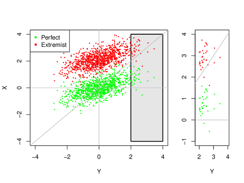
Figure 1: The sample illustrates the conditional distribution of the perfect forecast (green) and the extremist forecast (red) given the observation in the setting of eq. (1.1) and Table 2, where $\sigma^{2}=\frac{2}{3}$. The vertical stripe, which is enlarged at right, corresponds to cases where the respective point forecast exceeds a threshold value of 2.

In contrast, the interpretation of the second component $[F|Y]$ in the likelihood-baserate factorization (2.2) is much less clear. While the conditional distribution of the forecast given the observation can be viewed as a measure of discrimination ability, it was noted by Murphy and Winkler (1987) that forecasts can be perfectly discriminatory although they are uncalibrated. Therefore, discrimination ability by itself is not informative, and forecast assessment might be misguided if one stratifies by the realized value of the observation. To demonstrate this, we return to the simpler setting of point forecasts and revisit the simulation example of eq. (1.1) and Table 2, with $\sigma^{2}=\frac{2}{3}$ being fixed. Figure 1 shows the perfect forecast, the deliberately misspecified extremist forecast, and the observation in this setting. The bias of the extremist forecast is readily seen when all forecast cases are taken into account. However, if we restrict attention to cases where the observation exceeds a high threshold of 2, it is not obvious whether the perfect or the extremist forecast is preferable.

In this simple example, we have seen that if we stratify by the value of the realized observation, a deliberately misspecified forecast may appear appealing, while an ideal forecast may appear flawed, even though the forecasts are based on the same information set. Fortunately, unwanted effects of this type are avoided if we stratify by the value of the forecast. To see this, note that ideal predictive distributions and their induced point forecasts satisfy the auto-calibration property (2.3) and, subject to conditions, the unbiasedness property (2.4), respectively.

2.2 Proper scoring rules and consistent scoring functions

In the previous section we have introduced calibration and sharpness as key aspects of the quality of probabilistic forecasts. Proper scoring rules assess calibration and sharpness simultaneously and play key roles in the comparative evaluation and ranking of competing forecasts (Gneiting and Raftery, 2007). Specifically, let $\mathcal{F}$ denote a class of probability distributions on $\Omega_{Y}$, the set of possible values of the observation $Y$. A scoring rule is a mapping ${\rm S}:\mathcal{F}\times\Omega_{Y}\longrightarrow\mathbb{R}\cup\{\infty\}$ that assigns a numerical penalty based on the predictive distribution $F\in\mathcal{F}$ and observation $y\in\Omega_{Y}$. Generally, we identify a predictive distribution with its CDF. A scoring rule is proper relative to the class $\mathcal{F}$ if

$$\mathbb{E}_{G}\,{\rm S}(G,Y)\leq\mathbb{E}_{G}\,{\rm S}(F,Y)$$ (2.5)

for all probability distributions $F,G\in\mathcal{F}$. It is strictly proper relative to the class $\mathcal{F}$ if the above holds with equality only if $F=G$. In what follows we assume that $\Omega_{Y}=\mathbb{R}$. Scoring rules provide summary measures of predictive performance, and in practical applications, competing forecasting methods are compared and ranked in terms of the mean score over the cases in a test set. Propriety is a critically important element that encourages honest and careful forecasting, as the expected score is minimized if the quoted predictive distribution agrees with the actually assumed, under which the expectation in (2.5) is computed.

The most popular proper scoring rules for real-valued quantities are the logarithmic score (LogS), defined as

$$\textnormal{LogS}(F,y)=-\log f(y),$$ (2.6)

where $f$ denotes the density of $F$ (Good, 1952), which applies to absolutely continuous distributions only, and the continuous ranked probability score (CRPS), which is defined as

$$\textnormal{CRPS}(F,y)=\int_{-\infty}^{\infty}\left(F(z)-\mathbbm{1}\{y\leq z\}\right)^{2}\>\textup{d}z$$ (2.7)

directly in terms of the predictive CDF (Matheson and Winkler, 1976). The CRPS can be interpreted as the integral of the proper Brier score (Brier, 1950; Gneiting and Raftery, 2007),

$$\textnormal{BS}_{z}(F,y)=\left(F(z)-\mathbbm{1}\{y\leq z\}\right)^{2},$$ (2.8)

for the induced probability forecast for the binary event of the observation not exceeding the threshold value $z$. Alternative respresentations of the CRPS are discussed in Gneiting and Raftery (2007) and Gneiting and Ranjan (2011).

The quality of point forecasts is typically assessed by means of a scoring function ${\rm s}(x,y)$ that assigns a numerical score based on the point forecast, $x$, and the respective observation, $y$. As in the case of proper scoring rules, competing forecasting methods are compared and ranked in terms of the mean score over the cases in a test set. Popular scoring functions include the squared error, ${\rm s}(x,y)=(x-y)^{2}$, and the absolute error, ${\rm s}(x,y)=|x-y|$, for which we have reported mean scores in Table 2.

To avoid misguided inferences, the scoring function and the forecasting task have to be matched carefully, either by specifying the scoring function ex ante, or by employing scoring functions that are consistent for a target functional ${\rm T}$, relative to the class $\mathcal{F}$ of predictive distributions at hand, in the technical sense that

$$\mathbb{E}_{F}\,{\rm s}({\rm T}(F),Y)\leq\mathbb{E}_{F}\,{\rm s}(x,Y)$$

for all $x\in\mathbb{R}$ and $F\in\mathcal{F}$ (Gneiting, 2011). For instance, the squared error scoring function is consistent for the mean or expectation functional relative to the class of the probability measures with finite first moment, and the absolute error scoring function is consistent for the median functional.

Consistent scoring functions become proper scoring rules if the point forecast is chosen to be the Bayes rule or optimal point forecast under the respective predictive distribution. In other words, if the scoring function ${\rm s}$ is consistent for the functional ${\rm T}$, then

$${\rm S}(F,y)={\rm s}({\rm T}(F),y)$$

defines a proper scoring rule relative to the class $\mathcal{F}$. For instance, squared error can be interpreted as a proper scoring rule provided the point forecast is the mean of the respective predictive distribution, and absolute error yields a proper scoring rule if the point forecast is the median of the predictive distribution.

2.3 Understanding the forecaster’s dilemma

We are now in the position to analyze and understand the forecaster’s dilemma both within the joint distribution framework and from the perspective of proper scoring rules. While there is no unique definition of extreme events in the literature, we follow common practice and take extreme events to be observations that fall into the tails of the underlying population. In public discussions of the quality of forecasts, attention often falls exclusively on cases with extreme observations. As we have seen, under this practice even the most skillful forecasts available are bound to fail in the public eye, particularly when the signal-to-noise ratio in the data generating process is low. In a nutshell, if forecast evaluation is restricted to cases where the observation falls into a particular region of the outcome space, forecasters are encouraged to unduly emphasize this region.

Within the joint distribution framework of Section 2.1, any stratification by, and conditioning on, the realized values of the outcome is problematic and ought to be avoided, as general theoretical guidance for the interpretation and assessment of the resulting conditional distribution $[F|Y]$ does not appear to be available. In view of the likelihood-baserate factorization (2.2) of the joint distribution of the forecast and the observation, the forecaster’s dilemma arises as a consequence. Fortunately, stratification by, and conditioning on, the values of a point forecast or probabilistic forecast is unproblematic from a decision theoretic perspective, as the auto-calibration property (2.3) lends itself to practical tools and tests for calibration checks, as discussed by Gneiting et al. (2007), Held et al. (2010), and Strähl and Ziegel (2015), among others.

From the perspective of proper scoring rules, Gneiting and Ranjan (2011) showed that a proper scoring rule $S_{0}$ is rendered improper if the product with a non-constant weight function $w(y)$ is formed. Specifically, consider the weighted scoring rule

$${\rm S}(F,y)=w(y)\,{\rm S}_{0}(F,y).$$ (2.9)

Then if $Y$ has density $g$, the expected score $\mathbb{E}_{g}{\rm S}(F,Y)$ is minimized by the predictive distribution $F$ with density

$$f(y)=\frac{w(y)g(y)}{\int w(z)g(z)\,\textup{d}z},$$ (2.10)

which is proportional to the product of the weight function, $w$, and the true density, $g$. In other words, forecasters are encouraged to deviate from their true beliefs and misspecify their predictive densities, with multiplication by the weight function (and subsequent normalization) being an optimal strategy. Therefore, the scoring rule ${\rm S}$ in (2.9) is improper.

To connect to the forecaster’s dilemma, consider the indicator weight function $w_{r}(y)=\mathbbm{1}\{y\geq r\}$. The use of the weight function $w_{r}$ does not directly correspond to restricting the evaluation set to cases where the observation exceeds or equals the threshold value $r$, as instead of excluding these cases, a score of zero is assigned to them. However, when forecast methods are compared, the use of the indicator weighted scoring rule corresponds to a multiplicative scaling of the restricted score, and so the ranking of competing forecasts is the same as that obtained by restricting the evaluation set.

2.4 Tailoring proper scoring rules

The forecaster’s dilemma gives rise to the question how one might apply scoring rules to probabilistic forecasts when particular emphasis is placed on extreme events, while retaining propriety. To this end, Diks et al. (2011) and Gneiting and Ranjan (2011) consider the use of proper weighted scoring rules that emphasize specific regions of interest.

Diks et al. (2011) propose the conditional likelihood (CL) score,

$$\textnormal{CL}(F,y)=-w(y)\log\!\left(\frac{f(y)}{\int_{-\infty}^{\infty}w(z)f(z)\,\textup{d}z}\right)\!,$$ (2.11)

and the censored likelihood (CSL) score,

$$\textnormal{CSL}(F,y)=-w(y)\log f(y)-(1-w(y))\log\!\left(1-\int_{-\infty}^{\infty}w(z)f(z)\,\textup{d}z\right)\!.$$ (2.12)

Here, $w$ is a weight function such that $0\leq w(z)\leq 1$ and $\int w(z)f(z)\,\textup{d}z>0$ for all potential predictive distributions, where $f$ denotes the density of $F$. When $w(z)\equiv 1$, both the CL and the CSL score reduce to the unweighted logarithmic score (2.6). Gneiting and Ranjan (2011) propose the threshold-weighted continuous ranked probability score (twCRPS), defined as

$$\textnormal{twCRPS}(F,y)=\int_{-\infty}^{\infty}w(z)\left(F(z)-\mathbbm{1}\{y\leq z\}\right)^{2}\,\textup{d}z,$$ (2.13)

where, again, $w$ is a non-negative weight function. When $w(z)\equiv 1$, the twCRPS reduces to the unweighted CRPS (2.7). For recent applications of the twCRPS and a quantile-weighted version of the CRPS see, for example, Cooley et al. (2012), Lerch and Thorarinsdottir (2013) and Manzan and Zerom (2013).

As noted, these scoring rules are proper and can be tailored to the region of interest. When interest centers on the right tail of the distribution, we may choose $w(z)=\mathbbm{1}\{z\geq r\}$ for some high threshold $r$. However, the indicator weight function might result in violations of the regularity conditions for the CL and CSL scoring rule, unless all predictive densities considered are strictly positive. Furthermore, predictive distributions that are identical on $[r,\infty)$, but differ on $(-\infty,r)$, cannot be distinguished. Weight functions based on CDFs as proposed by Amisano and Giacomini (2007) and Gneiting and Ranjan (2011) provide suitable alternatives. For instance, we can set $w(z)=\Phi(z\,|\,r,\sigma^{2})$ for some $\sigma>0$, where $\Phi(\cdot\,|\,\mu,\sigma^{2})$ denotes the CDF of a normal distribution with mean $\mu$ and variance $\sigma^{2}$. Weight functions emphasizing the left tail of the distribution can be constructed similarly, by using $w(z)=\mathbbm{1}\{z\leq r\}$ or $w(z)=1-\Phi(z\,|\,r,\sigma^{2})$ for some low threshold $r$. In practice, the weighted integrals in (2.11), (2.12), and (2.13) may need to be approximated by discrete sums, which corresponds to the use of a discrete weight measure, rather than a weight function, as discussed by Gneiting and Ranjan (2011).

In what follows we focus on the above proper variants of the LogS and the CRPS. However, further types of proper weighted scoring rules can be developed. Pelenis (2014) introduces the penalized weighted likelihood score and the incremental CPRS. Tödter and Ahrens (2012) and Juutilainen et al. (2012) propose a logarithmic scoring rule that depends on the predictive CDF rather than the predictive density. As hinted at by Juutilainen et al. (2012, p. 466), this score can be generalized to a weighted version, which we call the threshold-weighted continuous ranked logarithmic score (twCRLS),

$$\textnormal{twCRLS}(F,y)=-\int_{\mathbb{R}}w(z)\log|F(z)-\mathbbm{1}\{y>z\}|\,\textup{d}z.$$ (2.14)

In analogy to the twCRPS (2.13) being a weighted integral of the Brier score in (2.8), the twCRLS (2.14) can be interpreted as a weighted integral of the discrete logarithmic score (LS) (Good, 1952; Gneiting and Raftery, 2007),

$$\textnormal{LS}_{z}(F,y) =-\log|F(z)-\mathbbm{1}\{y>z\}|$$ (2.15)

$$=-\mathbbm{1}\{y\leq z\}\log F(z)-\mathbbm{1}\{y>z\}\log\!\left(1-F(z)\right)\!,$$

for the induced probability forecast for the binary event of the observation not exceeding the threshold value $z$. The aforementioned weight functions and discrete approximations can be employed.

2.5 Diebold-Mariano tests

Formal statistical tests of equal predictive performance have been widely used, particularly in the economic literature. Turning now to a time series setting, we consider probabilistic forecasts $F_{t}$ and $G_{t}$ for an observation $y_{t+k}$ that lies $k$ time steps ahead. Given a proper scoring rule ${\rm S}$, we denote the respective mean scores on a test set ranging from time $t=1,\dots,n$ by

$$\bar{\rm S}^{F}_{n}=\frac{1}{n}\sum_{t=1}^{n}{\rm S}(F_{t},y_{t+k})\qquad\textnormal{and}\qquad\bar{\rm S}^{G}_{n}=\frac{1}{n}\sum_{t=1}^{n}{\rm S}(G_{t},y_{t+k}),$$

respectively. Diebold and Mariano (1995) proposed the use of the test statistic

$$t_{n}=\sqrt{n}\,\frac{\bar{\rm S}^{F}_{n}-\bar{\rm S}^{G}_{n}}{\hat{\sigma}_{n}},$$ (2.16)

where $\hat{\sigma}_{n}^{2}$ is a suitable estimator of the asymptotic variance of the score difference. Under the null hypothesis of a vanishing expected score difference and standard regularity conditions, the test statistic $t_{n}$ in (2.16) is asymptotically standard normal (Diebold and Mariano, 1995; Giacomini and White, 2006; Diebold, 2015). When the null hypothesis is rejected in a two-sided test, $F$ is preferred if the test statistic $t_{n}$ is negative, and $G$ is preferred if $t_{n}$ is positive.

For $j=0,1,\ldots$ let $\hat{\gamma}_{j}$ denote the lag $j$ sample autocovariance of the sequence ${\rm S}(F_{1},y_{1+k})-{\rm S}(G_{1},y_{1+k}),\ldots,{\rm S}(F_{n},y_{n+k})-{\rm S}(G_{n},y_{n+k})$ of score differences. Diebold and Mariano (1995) noted that for ideal forecasts at the $k$ step ahead prediction horizon the respective errors are at most $(k-1)$-dependent. Motivated by this fact, Gneiting and Ranjan (2011) use the estimator

$$\hat{\sigma}_{n}^{2}=\begin{cases}\hat{\gamma}_{0}&\textnormal{if }k=1,\\ \hat{\gamma}_{0}+2\sum_{j=1}^{k-1}\hat{\gamma}_{j}&\textnormal{if }k\geq 2.\end{cases}$$ (2.17)

for the asymptotic variance in the test statistic (2.16). While the at most $(k-1)$-dependence assumption might be violated in practice for various reasons, this appears to be a reasonable and practically useful choice nonetheless. Diks et al. (2011) propose the use of the heteroskedasticity and autocorrelation consistent (HAC) estimator

$$\hat{\sigma}_{n}^{2}=\hat{\gamma}_{0}+2\sum_{j=1}^{J}\!\left(1-\frac{j}{J}\right)\!\hat{\gamma}_{j},$$ (2.18)

where $J$ is the largest integer less than or equal to $n^{1/4}$. When this latter estimator is used, larger estimates of the asymptotic variance and smaller absolute values of the test statistic (2.16) tend to be obtained, as compared to using the estimator (2.17), particularly when the sample size $n$ is large.

3 Simulation studies

We now present simulation studies. In Section 3.1 we mimic the experiment reported on in Table 2 for point forecasts, now illustrating the forecaster’s dilemma on probabilistic forecasts. Furthermore, we consider the influence of the signal-to-noise ratio in the data generating process. Thereafter in the following Sections, we investigate whether or not there is a case for the use of proper weighted scoring rules, as opposed to their unweighted counterparts, when interest focuses on extremes. As it turns out, the fundamental lemma of Neyman and Pearson (1933) provides theoretical guidance in this regard. All results in this section are based on 10 000 replications.

3.1 The influence of the signal-to-noise ratio

Let us recall that in the simulation setting of eq. (1.1) the observation satisfies $Y|\,\mu\sim\mathcal{N}(\mu,\sigma^{2})$ where $\mu\sim\mathcal{N}(0,1-\sigma^{2})$. In Table 2 we have considered three competing point forecasts — termed the perfect, unconditional, and extremist forecasts — and have noted the appearance of the forecaster’s dilemma when the quality of the forecasts is assessed on cases of extreme outcomes only.

Table 3: Mean scores for the probabilistic forecasts in Table 2, where the observation $Y$ satisfies (1.1) with $\sigma^{2}=\frac{2}{3}$ being fixed. The CRPS and LogS are computed based on all observations, whereas the restricted versions (rCRPS and rLogS) are based on observations exceeding 1.64, the 95th percentile of the population, only. The lowest value in each column is shown in bold.

Forecast	CRPS	LogS	rCRPS	rLogS
Perfect	0.46	1.22	0.96	2.30
Unconditional	0.57	1.42	1.48	3.03
Extremist	2.05	5.90	0.79	1.88

Table 4: Mean scores for the probabilistic forecasts in Table 2, where the observation $Y$ satisfies (1.1) with $\sigma^{2}=\frac{2}{3}$ being fixed, under the proper weighted scoring rules twCRPS, CL, and CSL. For each weight function and column, the lowest value is shown in bold.

Threshold $r$	Forecast	twCRPS	CL	CSL
Indicator weight function, $w(z)=\mathbbm{1}\{z\geq 1.64\}$
1.64	Perfect	0.018	$<$ 0.001	0.164
	Unconditional	0.019	$\hphantom{<}0.002$	0.204
	Extremist	0.575	$\hphantom{<}0.093$	2.205
Gaussian weight function, $w_{r}(z)=\Phi(z\,|\,1.64,1)$
1.64	Perfect	0.053	$-$0.043	0.298
	Unconditional	0.062	$-0.028$	0.345
	Extremist	0.673	$-$0.379	1.625

We now turn to probabilistic forecasts and study the effect of the parameter $\sigma\in(0,1)$ that governs predictability. Small values of $\sigma$ correspond to high signal-to-noise ratios, and large values of $\sigma$ to small signal-to-noise ratios, respectively. Marginally, $Y$ is standard normal for all values of $\sigma$. In the limit as $\sigma\to 0$ the perfect predictive distribution approaches the point measure in the random mean $\mu$; as $\sigma\to 1$ it approaches the unconditional standard normal distribution. The perfect probabilistic forecast is ideal in the technical sense of Section 2.1 and thus will be preferred over any other predictive distribution (with identical information basis) by any rational user (Diebold et al., 1998; Tsyplakov, 2013).

In Table 4 we report mean scores for the three probabilistic forecasts when $\sigma^{2}=\frac{2}{3}$ is fixed. Under the CRPS and LogS the perfect forecast outperforms the others, as expected, and the extremist forecast performs by far the worst. However, these results change drastically if cases with extreme observations are considered only. In analogy to the results in Table 2, the perfect forecast is discredited under the restricted scores rCRPS and rLogS, whereas the misguided extremist forecast appears to excel, thereby demonstrating the forecaster’s dilemma in the setting of probabilistic forecasts. As shown in Table 4, under the proper weighted scoring rules introduced in Section 2.4 with weight functions that emphasize the right tail, the rankings under the unweighted CRPS and LogS are restored.

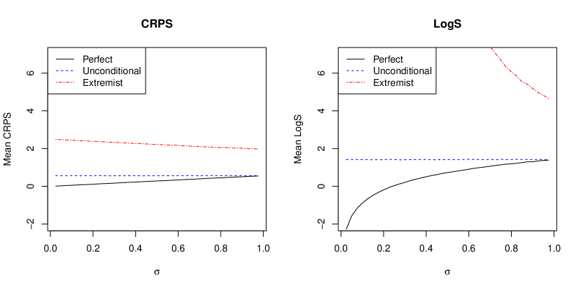
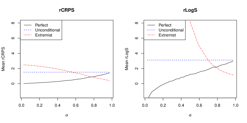
Figure 2: Mean CRPS and LogS for the probabilistic forecasts in the setting of eq. (1.1) and Table 2 as functions of the parameter $\sigma\in(0,1)$.

Figure 3: Mean of the improper restricted scoring rules rCRPS and rLogS for the probabilistic forecasts in the setting of eq. (1.1) and Table 2 as functions of the parameter $\sigma\in(0,1)$. The restricted mean scores are based on the subset of observations exceeding 1.64 only.

Next we investigate the influence of the signal-to-noise ratio in the data generating process on the appearance and extent of the forecaster’s dilemma. As noted, predictability increases with the parameter $\sigma\in(0,1)$. Figure 3 shows the mean CRPS and LogS for the three probabilistic forecasts as a function of $\sigma$. The scores for the unconditional forecast do not depend on $\sigma$. The predictive performance of the perfect forecast decreases in $\sigma$, which is natural, as it is less beneficial to know the value of $\mu$ when $\sigma$ is large. The extremist forecast yields better scores as $\sigma$ increases, which can be explained by the increase in the predictive variance that allows for a better match between the probabilistic forecast and the true distribution. For the improper restricted scoring rules rCRPS and rLogS, the same general patterns can be observed in Figure 3 — the mean score increases in $\sigma$ for the perfect forecast and decreases for the extremist forecast. In accordance with the forecaster’s dilemma, the extremist forecast is now perceived to outperform its competitors for all sufficiently large values of $\sigma$. However, for small values of $\sigma$, when the signal in $\mu$ is strong, the rankings are the same as under the CRPS and LogS in Figure 3. This illustrates the intuitively obvious observation that the forecaster’s dilemma is tied to stochastic systems with moderate to low signal-to-noise ratios, so that predictability is weak.

3.2 Power of Diebold-Mariano tests: Diks et al. (2011) revisited

While thus far we have illustrated the forecaster’s dilemma, the unweighted CRPS and LogS are well able to distinguish between the perfect forecast and its competitors. In the subsequent sections we investigate whether there are benefits to using proper weighted scoring rules, as opposed to their unweighted versions.

To begin with, we adopt the simulation setting in Section 4 of Diks et al. (2011). Suppose that at time $t=1,\ldots,n$, the observations $y_{t}$ are independent standard normal. We apply the two-sided Diebold-Mariano test of equal predictive performance to compare the ideal probabilistic forecast, the standard normal distribution, to a misspecified competitor, a Student $t$ distribution with five degrees of freedom, mean 0, and variance 1. Following Diks et al. (2011), we use the nominal level $0.05$, the variance estimate (2.18), and the indicator weight function $w(z)=\mathbbm{1}\{z\leq r\}$, and we vary the sample size, $n$, with the threshold value $r$ in such a way that under the standard normal distribution the expected number, $c=5$, of observations in the relevant region $(-\infty,r]$ remains constant.

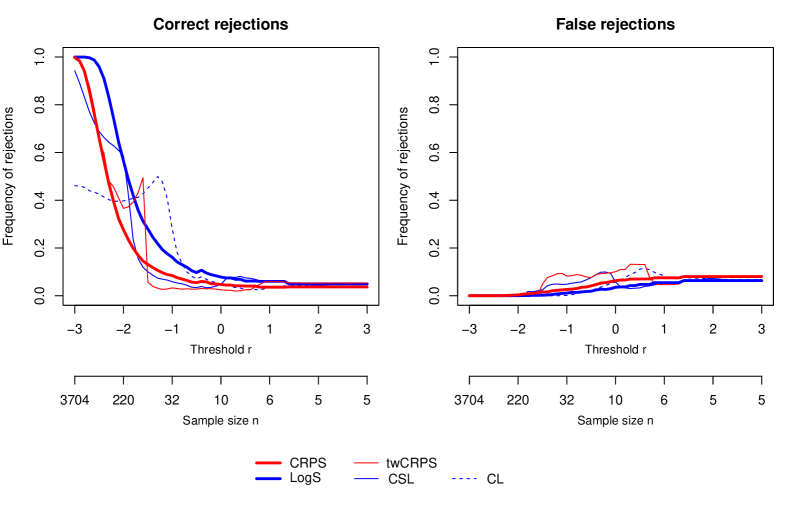
Figure 4: Frequency of correct rejections (in favor of the standard normal distribution, left panel) and false rejections (in favor of the Student $t$ distribution, right panel) in two-sided Diebold-Mariano tests in the simulation setting described in Section 3.2. The panels correspond to those in the left hand column of Figure 5 in Diks et al. (2011). The sample size $n$ for the tests depends on the threshold $r$ in the indicator weight function $w(z)=\mathbbm{1}\{z\leq r\}$ for the twCRPS, CL, and CSL scoring rules such that under the standard normal distribution there are five expected observations in the relevant interval $(-\infty,r]$.

Figure 4 shows the proportion of rejections of the null hypothesis of equal predictive performance in favor of either the standard normal or the Student $t$ distribution, respectively, as a function of the threshold value $r$ in the weight function. Rejections in favor of the standard normal distribution represent true power, whereas rejections in favor of the misspecified Student $t$ distribution are misguided. The curves for the tests based on the twCRPS, CL, and CSL scoring rules agree with those in the left column of Figure 5 of Diks et al. (2011). At first sight, they might suggest that the use of the indicator weight function $w(z)=\mathbbm{1}\{z\leq r\}$ with emphasis on the extreme left tail, as reflected by increasingly smaller values of $r$, yields increased power. At second sight, we need to compare to the power curves for tests using the unweighted CRPS and LogS, based on the same sample size, $n$, as corresponds to the threshold $r$ at hand. These curves suggest, perhaps surprisingly, that there may not be not be an advantage to using weighted scoring rules. To the contrary, the left-hand panel in Figure 4 suggests that tests based on the unweighted LogS are competitive in terms of statistical power.

3.3 The role of the Neyman-Pearson lemma

In order to understand this phenomenon, we follow the lead of Feuerverger and Rahman (1992) and draw a connection to a cornerstone of test theory, namely, the fundamental lemma of Neyman and Pearson (1933). In doing so we consider, for the moment, one-sided rather than two-sided tests.

In the simulation setting described by Diks et al. (2011) and in the previous section, any test of equal predictive performance can be re-interpreted as a test of the simple null hypothesis $H_{0}$ of a standard normal population against the simple alternative $H_{1}$ of a Student $t$ population. We write $f_{0}$ and $f_{1}$ for the associated density functions and $\mathbb{P}_{0}$ and $\mathbb{P}_{1}$ for probabilities under the respective hypotheses. By the Neyman-Pearson lemma (Lehmann and Romano, 2005, Theorem 3.2.1), under $H_{0}$ and at any level $\alpha\in(0,1)$ the unique most powerful test of $H_{0}$ against $H_{1}$ is the likelihood ratio test. The likelihood ratio test rejects $H_{0}$ if $\prod_{t=1}^{n}f_{1}(y_{t})/\prod_{t=1}^{n}f_{0}(y_{t})>k$ or, equivalently, if

$$\sum_{t=1}^{n}\log f_{1}(y_{t})-\sum_{t=1}^{n}\log f_{0}(y_{t})>\log k,$$ (3.1)

where the critical value $k$ is such that

$$\mathbb{P}_{0}\!\left(\frac{\prod_{t=1}^{n}f_{1}(y_{t})}{\prod_{t=1}^{n}f_{0}(y_{t})}>k\right)=\alpha.$$

Due to the optimality property of the likelihood ratio test, its power,

$$\mathbb{P}_{1}\!\left(\frac{\prod_{t=1}^{n}f_{1}(y_{t})}{\prod_{t=1}^{n}f_{0}(y_{t})}>k\right)\!,$$ (3.2)

gives a theoretical upper bound on the power of any test of $H_{0}$ versus $H_{1}$. Furthermore, the optimality result is robust, in the technical sense that minor misspecifications of either $H_{0}$ or $H_{1}$, as quantified by the Kullback-Leibler divergence, lead to minor loss of power only (Eguchi and Copas, 2006).

We now compare to the one-sided Diebold-Mariano test based on the logarithmic score (LogS; eq. 2.6). This test uses the statistic (2.16) and rejects $H_{0}$ if

$$\sum_{t=1}^{n}\log f_{1}(y_{t})-\sum_{t=1}^{n}\log f_{0}(y_{t})>\sqrt{n}\,\hat{\sigma}_{n}z_{1-\alpha},$$ (3.3)

where $z_{1-\alpha}$ is a standard normal quantile and $\hat{\sigma}_{n}^{2}$ is given by (2.17) or (2.18). Comparing with (3.1), we see that the one-sided Diebold-Mariano test that is based on the LogS has the same type of rejection region as the likelihood ratio test. However, the Diebold-Mariano test uses an estimated critical value, which may lead to a level less or greater than the nominal level, $\alpha$, whereas the likelihood ratio test uses the (in the practice of forecasting unavailable) critical value that guarantees the desired nominal level, $\alpha$.

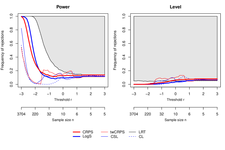
Figure 5: Power (left) and level (right) of the likelihood ratio test (LRT) and one-sided Diebold-Mariano tests in the simulation setting described in Section 3.2. The sample size $n$ for the tests depends on the threshold $r$ in the indicator weight function $w(z)=\mathbbm{1}\{z\leq r\}$ for the twCRPS, CL, and CSL scoring rules such that under the standard normal distribution there are five expected observations in the relevant interval $(-\infty,r]$. In the panel for power, the shaded area above the curve for the LRT corresponds to theoretically unattainable values for a test with nominal level. In the panel for level, the dashed line indicates the nominal level.

In this light, it is not surprising that the one-sided Diebold-Mariano test based on the LogS has power close to the theoretical optimum in (3.2). We illustrate this in Figure 5, where we plot the power and size of the likelihood ratio test and one-sided Diebold-Mariano tests based on the CRPS, twCRPS, LogS, CL, and CSL in the setting of the previous section. For small threshold values, the Diebold-Mariano test based on the unweighted LogS has much higher power than tests based on the weighted scores, even though it does not reach the power of the likelihood ratio test, which can be explained by the use of an estimated critical value and incorrect size properties. The theoretical upper bound on the power is violated by Diebold-Mariano tests based on the twCRPS and CL for threshold values between 0 and 1. However, the level of these tests exceeds the nominal level of $\alpha=0.05$ with too frequent rejections of $H_{0}$.

In the setting of two-sided tests, the connection to the Neyman-Pearson lemma is less straightforward, but the general principles remain valid and provide a partial explanation of the behavior seen in Figure 4.

3.4 Power of Diebold-Mariano tests: Further experiments

In the simulation experiments just reported, Diebold-Mariano tests based on proper weighted scoring rules generally are unable to outperform tests based on traditionally used, unweighted scoring rules. Several potential reasons come to mind. As we have just seen, when the true data generating process is given by one of the competing forecast distributions, the Neyman-Pearson lemma points at the superiority of tests based on the unweighted LogS. Furthermore, in the simulation setting considered thus far, the distributions considered differ both in the center, the left tail, and the right tail, and the test sample size varied with the threshold for the weight function in a peculiar way.

Therefore, we now consider a revised simulation setting, where we compare two forecast distributions neither of which corresponds to the true sampling distribution, where the forecast distributions only differ on the positive half-axis, and where the test sample size is fixed at $n=100$. The three candidate distributions are given by $\Phi$, a standard normal distribution with density $\phi$, by a heavy-tailed distribution $H$ with density

$$h(x)=\mathbbm{1}\{x\leq 0\}\,\phi(x)+\mathbbm{1}\{x>0\}\,\frac{3}{8}\left(1+\frac{x^{2}}{4}\right)^{-5/2},$$

and by an equally weighted mixture $F$ of $\Phi$ and $H$, with density

$$f(x)=\frac{1}{2}\left(\phi(x)+h(x)\right)\!.$$

We perform two-sided Diebold-Mariano tests of equal predictive performance based on the CRPS, twCRPS, LogS, CL, and CSL.

In Scenario A, the data are a sample from the standard normal distribution $\Phi$, and we compare the forecasts $F$ and $H$, respectively. In Scenario B, we interchange the roles of $\Phi$ and $H$, that is, the data are a sample from $H$, and we compare the forecasts $F$ and $\Phi$. The Neyman-Pearson lemma does not apply in this setting. However, the definition of $F$ as a weighted mixture of the true distribution and a misspecified competitor lets us expect that $F$ is to be preferred over the latter. Indeed, by Proposition 3 of Nau (1985), if $F=w\,G+(1-w)\,H$ with $w\in[0,1]$ is a convex combination of $G$ and $H$, then

$$\mathbb{E}_{G}\,{\rm S}(G,Y)\leq\mathbb{E}_{G}\,{\rm S}(F,Y)\leq\mathbb{E}_{G}\,{\rm S}(H,Y)$$

for any proper scoring rule ${\rm S}$. As any utility function induces a proper scoring rule via the respective Bayes act, this implies that under $G$ any rational decision maker favors $F$ over $H$ (Dawid, 2007; Gneiting and Raftery, 2007).

We estimate the frequencies of rejections of the null hypothesis of equal predictive performance at level $\alpha=0.05$. The choice of the estimator for the asymptotic variance of the score difference in the Diebold-Mariano test statistic (2.16) does not have a recognizable effect in this setting, and so we show results under the estimator (2.17) with $k=1$ only.

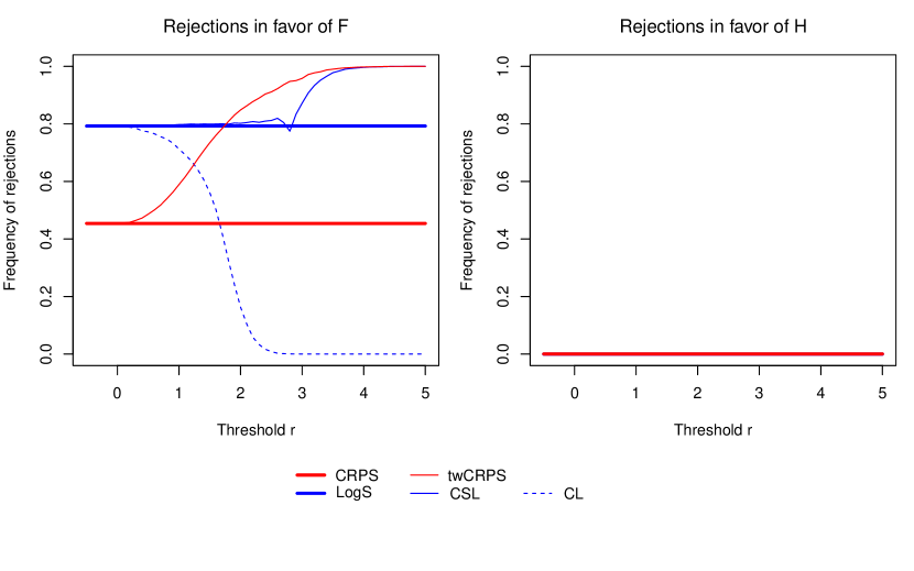
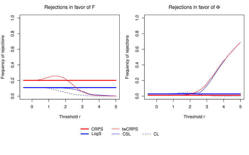
Figure 6: Scenario A in Section 3.4. The null hypothesis of equal predictive performance of $F$ and $H$ is tested under a standard normal population. The panels show the frequency of rejections in two-sided Diebold-Mariano tests in favor of either $F$ (left, desired) or $H$ (misguided, right). The tests under the twCRPS, CL, and CSL scoring rules use the weight function $w(z)=\mathbbm{1}\{z\geq r\}$, and the sample size is fixed at $n=100$.

Figure 7: Scenario B in Section 3.4. The null hypothesis of equal predictive performance of $F$ and $\Phi$ is tested under a Student $t$ population. The panels show the frequency of rejections in two-sided Diebold-Mariano tests in favor of either $F$ (desired, left) or $\Phi$ (misguided, right). The tests under the twCRPS, CL, and CSL scoring rules use the weight function $w(z)=\mathbbm{1}\{z\geq r\}$, and the sample size is fixed at $n=100$.

Figure 7 shows rejection rates under Scenario A in favor of $F$ and $H$, respectively, as a function of the threshold $r$ in the indicator weight function $w(z)=\mathbbm{1}\{z\geq r\}$ for the weighted scoring rules. The frequency of the desired rejections in favor of $F$ increases with larger thresholds for tests based on the twCRPS and CSL, thereby suggesting an improved discrimination ability at high threshold values. Under the CL scoring rule, the rejection rate decreases rapidly for larger threshold values. This can be explained by the fact that the weight function is a multiplicative component of the CL score in (2.11). As $r$ becomes larger and larger, none of the 100 observations in the test sample exceed the threshold, and so the mean scores under both forecasts vanish. This can also be observed in Figure 4, where, however, the effect is partially concealed by the increase of the sample size for more extreme threshold values. Interestingly, an issue very similar to that for the CL scoring rule arises in the assessment of deterministic forecasts of rare and extreme binary events, where performance measures based on contingency tables have been developed and standard measures degenerate to trivial values as events become rarer (Marzban, 1998; Stephenson et al., 2008), posing a challenge that has been addressed by Ferro and Stephenson (2011).

Figure 7 shows the respective rejection rates under Scenario B, where the sample is generated from the heavy-tailed distribution $H$, and the forecasts $F$ and $\Phi$ are compared. In contrast to the previous examples the Diebold-Mariano test based on the CRPS shows a higher frequency of the desired rejections in favor of $F$ than the test based on the LogS. However, for the tests based on proper weighted scoring rules, the frequency of the desired rejections in favor of $F$ decays to zero with increasing threshold value, and for the tests based on the twCRPS and CSL, the frequency of the undesired rejections in favor of $\Phi$ rises for larger threshold values.

This seemingly counterintuitive observation can be explained by the tail behavior of the forecast distributions, as follows. Consider the twCRPS and CSL with the indicator weight function $w(z)=\mathbbm{1}\{z\geq r\}$ and a threshold $r$ that exceeds the maximum of the given sample. In this case, the scores do not depend on the observations, and are solely determined by the respective tail probabilities, with the lighter tailed forecast distribution receiving the better score. In a nutshell, when the emphasis lies on a low-probability region with few or no observations, the forecaster assigning smaller probability to this region will be preferred. The traditionally used unweighted scoring rules do not depend on a threshold and thus do not suffer from this deficiency.

In comparisons of the mixture distribution $F$ and the lighter-tailed forecast distribution $\Phi$ this leads to a loss of finite sample discrimination ability of the proper weighted scoring rules as the threshold $r$ increases. This observation also suggests that any favorable finite sample behavior of the Diebold-Mariano tests based on weighted scoring rules in Scenario A might be governed by rejections due to the lighter tails of $F$ compared to $H$.

In summary, even though the simulation setting at hand was specifically tailored to benefit proper weighted scoring rules, these do not consistently perform better in terms of statistical power when compared to their unweighted counterparts. Any advantages vanish at increasingly extreme threshold values in case the actually superior distribution has heavier tails.

4 Case study

Based on the work of Clark and Ravazzolo (2015), we compare probabilistic forecasting models for key macroeconomic variables for the United States, serving to demonstrate the forecaster’s dilemma and the use of proper weighted scoring rules in an application setting.

4.1 Data

We consider time series of quarterly gross domestic product (GDP) growth, computed as 100 times the log difference of real GDP, and inflation in the GDP price index (henceforth inflation), computed as 100 times the log difference of the GDP price index, over an evaluation period from the first quarter of 1985 to the second quarter of 2011, as illustrated in Figure 8. The data are available from the Federal Reserve Bank of Philadelphia’s real time dataset.

Figure 8: Observations of GDP growth and inflation in the U.S. from the first quarter of 1985 to the second quarter of 2011. Solid circles indicate observations considered here as extreme events.

For each quarter $t$ in the evaluation period, we use the real-time data vintage $t$ to estimate the forecasting models and construct forecasts for period $t$ and beyond. The data vintage $t$ includes information up to time $t-1$. The one-quarter ahead forecast is thus a current quarter ($t$) forecast, while the two-quarter ahead forecast is a next quarter ($t+1$) forecast, and so forth (Clark and Ravazzolo, 2015). Here we focus on forecast horizons of one and four quarters ahead.

As the GDP data are continually revised, it is not immediate which revision should be used as the realized observation. We follow Romer and Romer (2000) and Faust and Wright (2009) who use the second available estimates as the actual data. Specifically, suppose a forecast for quarter $t+k$ is issued based on the vintage $t$ data ending in quarter $t-1$. The corresponding realized observation is then taken from the vintage $t+k+2$ data set. This approach may entail structural breaks in case of benchmark revisions, but is comparable to real-world forecasting situations where noisy early vintages are used to estimate predictive models (Faust and Wright, 2009).

4.2 Forecasting models

We consider autoregressive (AR) and vector autoregressive (VAR) models, the specifications of which are given now. For further details and a discussion of alternative models, see Clark and Ravazzolo (2015).

Our baseline model is an AR($p$) scheme with constant shock variance. Under this model, the conditional distribution of $Y_{t}$ is given by

$$Y_{t}\,|\,\mathbf{y}_{<t},b_{0},\ldots,b_{p},\sigma\sim\mathcal{N}\left(b_{0}+\sum_{i=1}^{p}b_{i}y_{t-i},\sigma^{2}\right)\!,$$ (4.1)

where $p=2$ for GDP growth and $p=4$ for inflation. Here, $\mathbf{y}_{<t}$ denotes the vector of the realized values of the variable $Y$ prior to time $t$. We estimate the model parameters $b_{0},\ldots,b_{p}$ and $\sigma$ in a Bayesian fashion using Markov chain Monte Carlo (MCMC) under a recursive estimation scheme, where the data sample $\mathbf{y}_{<t}$ is expanded as forecasting moves forward in time. The predictive distribution then is the Gaussian variance-mean mixture

$$\frac{1}{m}\sum_{j=1}^{m}\mathcal{N}\!\left(b_{0,j}+\sum_{i=1}^{p}b_{i,j}y_{t-i},\,\sigma_{j}^{2}\right)\!,$$ (4.2)

where $m=5\,000$ and $(b_{0,1},\ldots,b_{p,1},\sigma_{1}),\ldots,(b_{0,m},\ldots,b_{p,m},\sigma_{m})$ is a sample from the posterior distribution of the model parameters. For the other forecasting models, we proceed analogously.

A more flexible approach is the Bayesian AR model with time-varying parameters and stochastic specification of the volatility (AR-TVP-SV) proposed by Cogley and Sargent (2005), which has the hierarchical structure given by

$$Y_{t}\,|\,\mathbf{y}_{<t},b_{0,t},\ldots,b_{p,t},\lambda_{t} \sim\mathcal{N}\!\left(b_{0,t}+\sum_{i=1}^{p}b_{i,t}y_{t-i},\,\lambda_{t}\right)\!,$$ (4.3)

$$b_{i,t}\,|\,b_{i,t-1},\tau \sim\mathcal{N}\!\left(b_{i,t-1},\tau^{2}\right)\!,\quad i=0,\ldots,p,$$

$$\log\lambda_{t}\,|\,\lambda_{t-1},\sigma \sim\mathcal{N}\!\left(\log\lambda_{t-1},\sigma^{2}\right)\!.$$

Again, we set $p=2$ for GDP growth and $p=4$ for inflation.

In a multivariate extension of the AR models, we consider VAR schemes where GDP growth, inflation, unemployment rate, and three-month government bill rate are modeled jointly. Specifically, the conditional distribution of the four-dimensional vector $\mathbf{Y}_{t}$ is given by the multivariate normal distribution

$$\mathbf{Y}_{t}\,|\,\mathbf{Y}_{<t},\mathbf{b}_{0},\mathbf{B}_{1},\ldots,\mathbf{B}_{p},{\boldsymbol{\Sigma}}\sim\mathcal{N}_{4}\!\left(\mathbf{b}_{0}+\sum_{i=1}^{p}\mathbf{B}_{i}\mathbf{y}_{t-1},{\boldsymbol{\Sigma}}\right)\!,$$ (4.4)

where $\mathbf{Y}_{<t}$ denotes the data prior to time $t$, ${\boldsymbol{\Sigma}}$ is a $4\times 4$ covariance matrix, $\mathbf{b}_{0}$ is a vector of intercepts, and $\mathbf{B}_{i}$ is a $4\times 4$ matrix of lag $i$ coefficients, where $i=1,\ldots,p$. Here we take $p=4$. The univariate predictive distributions for GDP growth and inflation arise as the respective margins of the multivariate posterior predictive distribution.

Finally, we consider a VAR model with time-varying parameters and stochastic specification of the volatility (VAR-TVP-SV), which is a multivariate extension of the AR-TVP-SV model (Cogley and Sargent, 2005). Let ${\boldsymbol{\beta}}_{t}$ denote the vector of size $4(4p+1)$ comprising the parameters $\mathbf{b}_{0,t}$ and $\mathbf{B}_{1,t},\ldots,\mathbf{B}_{p,t}$ at time $t$, set ${\boldsymbol{\Lambda}}_{t}=\textup{diag}(\lambda_{1,t},\ldots,\lambda_{4,t})$ and let $\mathbf{A}$ be a lower triangular matrix with ones on the diagonal and non-zero random coefficients below the diagonal. The VAR-TVP-SV model takes the hierarchical form

$$\mathbf{Y}_{t}\,|\,\mathbf{Y}_{<t},{\boldsymbol{\beta}}_{t},{\boldsymbol{\Lambda}}_{t},\mathbf{A} \sim\mathcal{N}_{4}\!\left(\mathbf{b}_{0,t}+\sum_{i=1}^{p}\mathbf{B}_{i,t}\mathbf{y}_{t-1},\mathbf{A}^{-1}{\boldsymbol{\Lambda}}_{t}(\mathbf{A}^{-1})^{\top}\right)\!,$$ (4.5)

$${\boldsymbol{\beta}}_{t}\,|\,{\boldsymbol{\beta}}_{t-1},\mathbf{Q} \sim\mathcal{N}_{4(4p+1)}\!\left({\boldsymbol{\beta}}_{t-1},\mathbf{Q}\right)\!,$$

$$\log\lambda_{i,t}\,|\,\lambda_{i,t-1},\sigma_{i} \sim\mathcal{N}\!\left(\log\lambda_{i,t-1},\sigma_{i}^{2}\right)\!,\quad i=1,\ldots,4.$$

We set $p=2$ and refer to Clark and Ravazzolo (2015) for further details of the notation, the model, and its estimation.

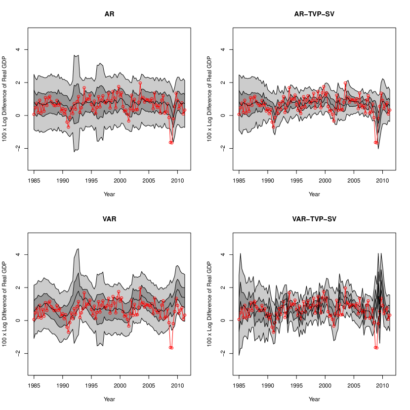
Figure 9: One-quarter ahead forecasts of U.S. GDP growth generated by the AR, AR-TVP-SV, VAR, and VAR-TVP-SV models. The median of the predictive distribution is shown in the black solid line, and the central 50% and 90% prediction intervals are shaded in dark and light gray, respectively. The red line shows the corresponding observations.

Figure 9 shows one-quarter ahead forecasts of GDP growth over the evaluation period. The baseline models with constant volatility generally exhibit wider prediction intervals, while the TVP-SV models show more pronounced fluctuations both in the median forecast and the associated uncertainty. In 1992 and 1996, the Bureau of Economic Analysis performed benchmark data revisions, which causes the prediction uncertainty of the baseline models to increase substantially. The more flexible TVP-SV models seem less sensitive to these revisions.

Table 5: Mean CRPS and mean LogS for probabilistic forecasts of GDP growth and inflation in the U.S. at prediction horizons of $k=1$ and $k=4$ quarters, respectively, for the first quarter of 1985 to the second quarter of 2011. For each variable and column, the lowest value is in bold.

	CRPS		LogS
	$k=1$	$k=4$	$k=1$	$k=4$
GDP Growth
AR	0.330	0.359	1.044	1.120
AR-TVP-SV	0.292	0.329	0.833	1.019
VAR	0.385	0.402	1.118	1.163
VAR-TVP-SV	0.359	0.420	0.997	1.257
Inflation
AR	0.167	0.187	0.224	0.374
AR-TVP-SV	0.143	0.156	0.047	0.175
VAR	0.170	0.198	0.235	0.428
VAR-TVP-SV	0.162	0.201	0.179	0.552

Table 6: Mean restricted CRPS (rCRPS) and restricted LogS (rLogS) for probabilistic forecasts of GDP growth and inflation in the U.S. at prediction horizons of $k=1$ and $k=4$ quarters, respectively, for the first quarter of 1985 to the second quarter of 2011. The means are computed on instances when the observation is smaller than 0.10 (GDP) or larger than 0.98 (inflation) only. For each variable and column, the lowest value is shown in bold.

	rCRPS		rLogS
	$k=1$	$k=4$	$k=1$	$k=4$
GDP Growth
AR	0.654	0.870	1.626	2.010
AR-TVP-SV	0.659	0.970	2.016	3.323
VAR	0.827	0.924	2.072	2.270
VAR-TVP-SV	0.798	0.978	2.031	2.409
Inflation
AR	0.214	0.157	0.484	0.296
AR-TVP-SV	0.236	0.179	0.619	0.327
VAR	0.203	0.147	0.424	0.317
VAR-TVP-SV	0.302	0.247	0.950	0.849

4.3 Results

To compare the predictive performance of the four forecasting models, Table 5 shows the mean CRPS and LogS over the evaluation period. For the LogS, we follow extant practice in the economic literature and employ the quadratic approximation proposed by Adolfson et al. (2007). Specifically, we find the mean, $\hat{\mu}_{F}$, and variance, $\hat{\sigma}^{2}_{F}$, of a sample $\hat{x}_{1},\dots,\hat{x}_{m}$, where $\hat{x}_{i}$ is a random number drawn from the $i$th mixture component of the posterior predictive distribution (4.2), and compute the logarithmic score under the assumption of a normal predictive distribution with mean $\hat{\mu}_{F}$ and variance $\hat{\sigma}^{2}_{F}$. To compute the CRPS and the threshold-weighted CRPS, we use the numerical methods proposed by Gneiting and Ranjan (2011).

The relative predictive performance of the forecasting models is consistent across the two variables and the two proper scoring rules. The AR-TVP-SV model has the best predictive performance and outperforms the baseline AR model. The $p$-values for the respective two-sided Diebold-Mariano tests range from 0.00 to 0.06, except for the LogS for GDP growth at a prediction horizon of $k=4$ quarters, where the $p$-value is 0.37. However, the VAR models fail to outperform the simpler AR models. As we do not impose sparsity constraints on the parameters of the VAR models, this is likely due to overly complex forecasting models and overfitting, in line with results of Holzmann and Eulert (2014) and Clark and Ravazzolo (2015) in related economic and financial case studies.

To relate to the forecaster’s dilemma, we restrict attention to extremes events. For GDP growth, we consider quarters with observed growth less than $r=0.1$ only. For inflation, we restrict attention to high values in excess of $r=0.98$. In either case, this corresponds to using about 10% of the observations. Table 6 shows the results of restricting the computation of the mean CRPS and the mean LogS to these observations only. For both GDP growth and inflation, the baseline AR model is considered best, and the AR-TVP-SV model appears to perform poorly. These restricted scores thus result in substantially different rankings than the proper scoring rules in Table 5, thereby illustrating the forecaster’s dilemma. Strikingly, under the restricted assessment all four models seem less skillful at predicting inflation in the current quarter than four quarters ahead. This is a counterintuitive result that illustrates the dangers of conditioning on outcomes and should be viewed as a further manifestation of the forecaster’s dilemma.

Table 7: Mean threshold-weighted CRPS for probabilistic forecasts of GDP growth and inflation in the U.S. at prediction horizons of $k=1$ and $k=4$ quarters, respectively, under distinct weight functions, for the first quarter of 1985 to the second quarter of 2011. For each variable and column, the lowest value is shown in bold.

	twCRPS
	$k=1$	$k=4$	$k=1$	$k=4$
GDP Growth	$w_{\textnormal{I}}(z)=\mathbbm{1}\{z\leq 0.1\}$		$w_{\textnormal{G}}=1-\Phi(z\,|\,0.1,1)$
AR	0.062	0.068	0.053	0.057
AR-TVP-SV	0.052	0.062	0.048	0.055
VAR	0.062	0.062	0.054	0.054
VAR-TVP-SV	0.059	0.080	0.053	0.065
Inflation	$w_{\textnormal{I}}(z)=\mathbbm{1}\{z\geq 0.98\}$		$w_{\textnormal{G}}=\Phi(z\,|\,0.98,1)$
AR	0.026	0.032	0.068	0.075
AR-TVP-SV	0.018	0.018	0.059	0.065
VAR	0.027	0.033	0.072	0.081
VAR-TVP-SV	0.022	0.037	0.067	0.081

In Table 7 we show results for the proper twCRPS under weight functions that emphasize the respective region of interest. For both variables, this yields rankings that are similar to those in Table 5. However, the $p$-values for binary comparisons with two-sided Diebold-Mariano tests generally are larger than those under the unweighted CRPS. The AR-TVP-SV model is predominantly the best, and the current quarter forecasts are deemed more skillful than those four quarters ahead.

5 Discussion

We have studied the dilemma that occurs when forecast evaluation is restricted to cases with extreme observations, a procedure that appears to be common practice in public discussions of forecast quality. As we have seen, under this practice even the most skillful forecasts available are bound to be discredited when the signal-to-noise ratio in the data generating process is low. Key examples might include macroeconomic and seismological predictions. In such settings it is important for forecasters, decision makers, journalists, and the general public to be aware of the forecaster’s dilemma. Otherwise, charlatanes might be given undue attention and recognition, and critical societal decisions could be based on misguided predictions.

We have offered two complementary explanations of the forecaster’s dilemma. From the joint distribution perspective of Section 2.1 stratifying by, and conditioning on, the realized value of the outcome is problematic in forecast evaluation, as theoretical guidance for the interpretation and assessment of the resulting conditional distributions is unavailable. In contrast stratifying by, and conditioning on, the forecast is unproblematic. From the perspective of proper scoring rules in 2.3, restricting the outcome space corresponds to the multiplication of the scoring rule by an indicator weight function, which renders any proper score improper, with an explicit hedging strategy being available.

Arguably the only remedy is to consider all available cases when evaluating predictive performance. Proper weighted scoring rules emphasize specific regions of interest and facilitate interpretation. Interestingly, however, the Neyman-Pearson lemma and our simulation studies suggest that in general the benefits of using proper weighted scoring rules in terms of power are rather limited, as compared to using standard, unweighted scoring rules. Any potential advantages vanish under weight functions with increasingly extreme threshold values, where the finite sample behavior of Diebold-Mariano tests depends on the tail properties of the forecast distributions only.

When evaluating probabilistic forecasts with emphasis on extremes, one could also consider functionals of the predictive distributions, such as the induced probability forecasts for binary tail events, as utilized in a recent comparative study by Williams et al. (2014). Another option is to consider the induced quantile forecasts, or related point summaries of the (tails of the) predictive distributions, at low or high levels, say $\alpha=0.975$ or $\alpha=0.99$, as is common practice in financial risk management, both for regulatory purposes and internally at financial institutions (McNeil et al., 2015). In this context, Holzmann and Eulert (2014) studied the power of Diebold-Mariano tests for quantile forecasts at extreme levels, and Fissler et al. (2015) raise the option of comparative backtests of Diebold-Mariano type in banking regulation. Ehm et al. (2016) propose decision theoretically principled, novel ways of evaluating quantile and expectile forecasts.

Variants of the forecaster’s dilemma have been discussed in various strands of literature. Centuries ago, Bernoulli (1713) argued that even the most foolish prediction might attract praise when a rare event happens to materialize, referring to lyrics by Owen (1607) that are quoted in the front matter of our paper.

Tetlock (2005) investigated the quality of probability forecasts made by human experts for U.S. and world events. He observed that while forecast quality is largely independent of an expert’s political views, it is strongly influenced by how a forecaster thinks. Forecasters who “know one big thing” tend to state overly extreme predictions and, therefore, tend to be outperformed by forecasters who “know many little things”. Furthermore, Tetlock (2005) found an inverse relationship between the media attention received by the experts and the accuracy of their predictions, and offered psychological explanations for the attractiveness of extreme predictions for both forecasters and forecast consumers. Media attention might thus not only be centered around extreme events, but also around less skillful forecasters with a tendency towards misguided predictions.

Denrell and Fang (2010) reported similar observations in the context of managers and entrepreneurs predicting the success of a new product. They also studied data from the Wall Street Journal Survey of Economic Forecasts, found a negative correlation between the predictive performance on a subset of cases with extreme observations and measures of general predictive performance based on all cases, and argued that accurately predicting a rare and extreme event actually is a sign of poor judgment. Their discussion was limited to point forecasts, and the suggested solution was to take into account all available observations, much in line with the findings and recommendations in our paper.

Appendix A Impropriety of quadratic approximations of weighted logarithmic scores

Let $F$ be a predictive distribution with mean $\mu_{F}$ and standard deviation $\sigma_{F}$. As regards the conditional likelihood (CL) score (2.11), the quadratic approximation is given by

$$\textnormal{CL}^{q}(F,y)=-w(y)\log\!\left(\frac{\phi(y|F)}{\int w(x)\phi(x|F)\,\textup{d}x}\right)\!,$$

where $\phi(\cdot|F)$ denotes a normal density with mean $\mu_{F}$ and standard deviation $\sigma_{F}$, respectively. Let

$$c_{F}=\int w(x)\phi(x|F)\,\textup{d}x,\qquad c_{G}=\int w(x)\phi(x|G)\,\textup{d}x,\qquad c_{g}=\int w(x)g(x)\,\textup{d}x,$$

and recall that the Kullback-Leibler divergence between two probability densities $u$ and $v$ is given by

$$K(u,v)=\int u(x)\log\!\left(\frac{u(x)}{v(x)}\right)\textup{d}x.$$

Assuming that CL^q is proper, it is true that

$$\mathbb{E}_{G} (\textnormal{CL}^{q}(F,Y)-\textnormal{CL}^{q}(G,Y))$$

$$=c_{g}\left[K\!\left(\frac{w(y)g(y)}{c_{g}},\frac{w(y)\phi(y|F)}{c_{F}}\right)-K\!\left(\frac{w(y)g(y)}{c_{g}},\frac{w(y)\phi(y|G)}{c_{G}}\right)\right]$$

is non-negative. Let $G$ be uniform on $[-\sqrt{3},\sqrt{3}]$ so that $\mu_{G}=0$ and $\sigma_{G}=1$, and let $w(y)=\mathbbm{1}\{y\geq 1\}$. Denoting the cumulative distribution function of the standard normal distribution by $\Phi$, we find that

$$K \!\left(\frac{w(y)g(y)}{c_{g}},\frac{w(y)\phi(y|F)}{c_{F}}\right)-K\!\left(\frac{w(y)g(y)}{c_{g}},\frac{w(y)\phi(y|G)}{c_{G}}\right)$$

$$=\log\!\left(\sigma_{F}\frac{1-\Phi((1-\mu_{F})/\sigma_{F})}{1-\Phi(1)}\right)+\frac{3(\sqrt{3}-1)\mu_{F}^{2}-6\mu_{F}+(3\sqrt{3}-1)(1-\sigma_{F}^{2})}{6(\sqrt{3}-1)\sigma_{F}^{2}},$$

which is strictly negative in a neighborhood of $\mu_{F}=1.314$ and $\sigma_{F}=0.252$, for the desired contradiction. Therefore, CL^q is not a proper scoring rule.

As regards the censored likelihood (CSL) score (2.12), the quadratic approximation is

$$\textnormal{CSL}^{q}(F,y)=-w(y)\log\!\left(\phi(y|F)\right)-(1-w(y))\log\!\left(1-\int w(z)\phi(z|F)\,\textup{d}z\right)\!.$$

Under the same choice of $w$, $F$, and $G$ as before, we find that

$$\mathbb{E}_{G} (\textnormal{CSL}^{q}(F,Y)-\textnormal{CSL}^{q}(G,Y))$$

$$=\frac{\sqrt{3}-1}{2\sqrt{3}}\log\sigma_{F}-\frac{\sqrt{3}+1}{2\sqrt{3}}\log\!\left(\frac{\Phi((1-\mu_{F})/\sigma_{F})}{\Phi(1)}\right)$$

$$\hskip 42.67912pt+\frac{3(\sqrt{3}-1)\mu_{F}^{2}-6\mu_{F}+(3\sqrt{3}-1)(1-\sigma_{F}^{2})}{12\sqrt{3}\,\sigma_{F}^{2}},$$

which is strictly negative in a neighborhood of $\mu_{F}=0.540$ and $\sigma_{F}=0.589$. Therefore, CSL^q is not a proper scoring rule.

Appendix B Online supplement: Media attention on extreme events

Table 8: Media coverage illustrating the focus on extreme events in public discussions of the quality of forecasts. The sources were accessed August 8, 2015.

Year	Headline	Source
2008	Dr. Doom	The New York Times
2009	How did economists get it so wrong?	The New York Times
2009	He told us so	The Guardian
2010	Experts who predicted US economy crisis see recovery	Bloomberg
2010	An exclusive interview with Med Yones - The expert who	CEO Q Magazine
	predicted the financial crisis
2011	A seer on banks raises a furor on bonds	The New York Times
2013	Meredith Whitney redraws ’map of prosperity’	USA Today
2007	Lessons learned from Great Storm	BBC
2011	Bad data failed to predict Nashville Flood	NBC
2012	Bureau of Meteorology chief says super storm ‘just blew up	The Courier-Mail
	on the city’
2013	Weather Service faulted for Sandy storm surge warnings	NBC
2013	Weather Service updates criteria for hurricane warnings,	Washington Post
	after Sandy criticism
2015	National Weather Service head takes blame for forecast	NBC
	failures
2011	Italian scientists on trial over L’Aquila earthquake	CNN
2011	Scientists worry over ‘bizarre’ trial on earthquake	Scientific American
	prediction
2012	L’Aquila ruling: Should scientists stop giving advice?	BBC

• http://www.nytimes.com/2008/08/17/magazine/17pessimist-t.html?pagewanted=all

• http://www.nytimes.com/2009/09/06/magazine/06Economic-t.html?_r=1&pagewanted=all

• http://www.guardian.co.uk/business/2009/jan/24/nouriel-roubini-credit-crunch

• http://www.bloomberg.com/apps/news?pid=conewsstory&refer=conews&tkr=K:US&sid=asziFnEsJSos

• http://www.ceoqmagazine.com/whopredictedfinancialcrisis/index.htm

• http://www.nytimes.com/2011/02/08/business/economy/08whitney.html?pagewanted=all&_r=0

• http://www.usatoday.com/story/money/business/2013/06/05/meredith-whitney-book-interview/2384905/

• http://news.bbc.co.uk/2/hi/science/nature/7044050.stm

• http://www.nbc15.com/weather/headlines/January_13_Report_Bad_Data_Failed_To_Predict_Nashville_Flood_113450314.html

• http://www.couriermail.com.au/news/queensland/bureau-of-meteorology-under-fire-after-a-weekend-of-wild-weather-and-storms-in-queensland-left-many-unprepared/story-e6freoof-1226519213928

• http://www.nbcnewyork.com/news/local/Sandy-Report-Weather-Storm-Surge-Warnings-207545031.html

• http://www.washingtonpost.com/blogs/capital-weather-gang/wp/2013/04/04/weather-service-changes-criteria-for-hurricane-warnings-after-sandy-criticism/

• http://www.nbcnews.com/storyline/blizzard-15/national-weather-service-head-takes-blame-forecast-failures-n294701

• http://articles.cnn.com/2011-09-20/world/world_europe_italy-quake-trial_1_geophysics-and-vulcanology-l-aquila-seismic-activity?_s=PM:EUROPE

• http://www.scientificamerican.com/article.cfm?id=trial-such-as-that-star

• http://www.bbc.co.uk/news/magazine-20097554

References

- Adolfson et al. (2007) Adolfson, M., Linde, J. and Villani, M. (2007). Forecasting performance of an open economy DSGE model. Econometric Reviews, 26 289–328.
- Albeverio et al. (2006) Albeverio, S., Jentsch, V. and Kantz, H. (eds.) (2006). Extreme Events in Nature and Society. Springer.
- Amisano and Giacomini (2007) Amisano, G. and Giacomini, R. (2007). Comparing density forecasts via weighted likelihood ratio tests. Journal of Business and Economic Statistics, 25 177–190.
- Beirlant et al. (2004) Beirlant, J., Goegebeur, Y., Teugels, J. and Segers, J. (2004). Statistics of Extremes. John Wiley & Sons, Chichester.
- Bernoulli (1713) Bernoulli, J. (1713). Ars Conjectandi. Impensis Thurnisiorum, Basileae. Reproduction of original from Sterling Memorial Library, Yale University. Online edition of Gale Digital Collections: The Making of the Modern World: Part I: The Goldsmiths’-Kress Collection, 1450-1850. Available at http://nbn-resolving.de/urn%3Anbn%3Ade%3Agbv%3A3%3A1-146753.
- Bernoulli (2006) Bernoulli, J. (2006). The Art of Conjecturing, together with Letter to a Friend on Sets in Court Tennis, translated and with an introduction and notes by Edith Dudley Sylla. John Hopkins Univ. Press, Baltimore.
- Brier (1950) Brier, G. W. (1950). Verification of forecasts expressed in terms of probability. Monthly Weather Review, 78 1–3.
- Clark and Ravazzolo (2015) Clark, T. E. and Ravazzolo, F. (2015). Macroeconomic forecasting performance under alternative specifications of time-varying volatility. Journal of Applied Econometrics, 30 551–575.
- Cogley and Sargent (2005) Cogley, T. S. M. and Sargent, T. J. (2005). Drifts and volatilities: Monetary policies and outcomes in the post-World War II U.S. Review of Economic Dynamics, 8 262–302.
- Coles (2001) Coles, S. (2001). An Introduction to Statistical Modeling of Extreme Values. Springer, London.
- Cooley et al. (2012) Cooley, D., Davis, R. A. and Naveau, P. (2012). Approximating the conditional density given large observed values via a multivariate extremes framework, with application to environmental data. The Annals of Applied Statistics, 6 1406–1429.
- Dawid (2007) Dawid, A. P. (2007). The geometry of proper scoring rules. Annals of the Institute of Statistical Mathematics, 59 77–93.
- Dawid and Sebastiani (1999) Dawid, A. P. and Sebastiani, P. (1999). Coherent dispersion criteria for optimal experimental design. The Annals of Statistics, 27 65–81.
- Denrell and Fang (2010) Denrell, J. and Fang, C. (2010). Predicting the next big thing: Success as a signal of poor judgment. Management Science, 56 1653–1667.
- Diebold (2015) Diebold, F. X. (2015). Comparing predictive accuracy, twenty years later: A personal perspective on the use and abuse of Diebold–Mariano tests. Journal of Business & Economic Statistics, 33 1–9.
- Diebold et al. (1998) Diebold, F. X., Gunther, T. A. and Tay, A. S. (1998). Evaluating density forecasts with applications to financial risk management. International Economic Review, 39 863–883.
- Diebold and Mariano (1995) Diebold, F. X. and Mariano, R. S. (1995). Comparing predictive accuracy. Journal of Business and Economic Statistics, 13 253–263.
- Diks et al. (2011) Diks, C., Panchenko, V. and van Dijk, D. (2011). Likelihood-based scoring rules for comparing density forecasts in tails. Journal of Econometrics, 163 215–230.
- Easterling et al. (2000) Easterling, D. R., Meehl, G. A., Parmesan, C., Changnon, S. A., Karl, T. R. and Mearns, L. O. (2000). Climate extremes: Observations, modeling, and impacts. Science, 289 2068–2074.
- Eguchi and Copas (2006) Eguchi, S. and Copas, J. (2006). Interpreting Kullback-Leibler divergence with the Neyman-Pearson lemma. Journal of Multivariate Analysis, 97 2034–2040.
- Ehm et al. (2016) Ehm, W., Gneiting, T., Jordan, A. and Krüger, F. (2016). Of quantiles and expectiles: Consistent scoring functions, Choquet representations, and forecast rankings. Journal of the Royal Statistical Society, Series B (Statistical Methodology), 78 in press.
- Ehrman and Shugan (1995) Ehrman, C. M. and Shugan, S. M. (1995). The forecaster’s dilemma. Marketing Science, 14 123–147.
- Embrechts et al. (1997) Embrechts, P., Klüppelberg, C. and Mikosch, T. (1997). Modelling Extremal Events for Insurance and Finance. Springer, Berlin.
- Faust and Wright (2009) Faust, J. and Wright, J. H. (2009). Comparing Greenbook and reduced form forecasts using a large realtime dataset. Journal of Business and Economic Statistics, 27 468–479.
- Ferro and Stephenson (2011) Ferro, C. A. T. and Stephenson, D. B. (2011). Extremal dependence indices: Improved verification measures for deterministic forecasts of rare binary events. Weather and Forecasting, 26 699–713.
- Feuerverger and Rahman (1992) Feuerverger, A. and Rahman, S. (1992). Some aspects of probability forecasting. Communications in Statistics – Theory and Methods, 21 1615–1632.
- Fissler et al. (2015) Fissler, T., Ziegel, J. F. and Gneiting, T. (2015). Expected shortfall is jointly elicitable with value-at-risk: Implications for backtesting. Risk, December in press.
- Giacomini and White (2006) Giacomini, R. and White, H. (2006). Tests of conditional predictive ability. Econometrica, 74 1545–1578.
- Gneiting (2008) Gneiting, T. (2008). Editorial: Probabilistic forecasting. Journal of the Royal Statistical Society Series A (Statistics in Society), 171 319–321.
- Gneiting (2011) Gneiting, T. (2011). Making and evaluating point forecasts. Journal of the American Statistical Association, 106 746–762.
- Gneiting et al. (2007) Gneiting, T., Balabdaoui, F. and Raftery, A. E. (2007). Probabilistic forecasts, calibration and sharpness. Journal of the Royal Statistical Society Series B (Statistical Methodology), 69 243–268.
- Gneiting and Katzfuss (2014) Gneiting, T. and Katzfuss, M. (2014). Probabilistic forecasting. Annual Review of Statistics and Its Application, 1 125–151.
- Gneiting and Raftery (2007) Gneiting, T. and Raftery, A. E. (2007). Strictly proper scoring rules, prediction, and estimation. Journal of the American Statistical Association, 102 359–378.