Position-dependent mass, finite-gap systems, and supersymmetry

Abstract

The ordering problem in quantum systems with position-dependent mass (PDM) is treated by inclusion of the classically fictitious similarity transformation into the kinetic term. This provides a generation of supersymmetry with the first order supercharges from the kinetic term alone, while inclusion of the potential term allows also to generate nonlinear supersymmetry with higher order supercharges. A broad class of finite-gap systems with PDM is obtained by different reduction procedures, and general results on supersymmetry generation are applied to them. We show that elliptic finite-gap systems of Lamé and Darboux-Treibich-Verdier types can be obtained by reduction to Seiffert’s spherical spiral and Bernoulli lemniscate in the presence of Calogero-like or harmonic oscillator potentials, or by angular momentum reduction of a free motion on some $AdS_{2}$-related surfaces in the presence of Aharonov-Bohm flux. The limiting cases include the Higgs and Mathews-Lakshmanan oscillator models as well as a reflectionless model with PDM exploited recently in the discussion of cosmological inflationary scenarios.

1 Introduction

Quantum mechanical systems with position-dependent mass (PDM) appear in physics in various contexts. When a particle interacts with an external environment, its mass is replaced by an effective mass that in general depends on the position. As a result, quantum systems with PDM emerge naturally in solid state physics where heterostructures are characterized by electrons’ effective masses [1, 2, 3, 4, 5]. In another way, they can be generated via a dimensional reduction of field-theoretical nonlinear sigma models and in a related framework of gravitation [6, 7, 8, 9, 10]. A certain class of such systems is used particularly in cosmological inflationary models [11]. Quantum mechanical systems with PDM were employed recently in the context of integrable models [12]. They turn out to be interesting from the point of view of supersymmetric quantum mechanics [13, 14, 15, 16, 17], coherent states [18, 19, 20], and PT-symmetry [21, 22, 23]. Besides the one-dimensional quantum systems with PDM, their multi-dimensional generalizations are considered in the literature [24, 25, 26, 27, 28, 29], particularly, in the context of superintegrable systems [30, 31]. See also refs. [32, 33, 34, 35, 36, 37, 38, 39, 40, 41, 42, 43, 44] where some other aspects of quantum systems with PDM were studied.

In treating quantum systems with PDM, there appears the ordering problem in the kinetic term. One can take a classical analog of such a system, remove the position dependence in the kinetic term via appropriate point (canonical) transformation, and then quantize the obtained system with translation-invariant kinetic term, the transformed potential term and, possibly, changed domain of the transformed coordinate variable. When working with such systems, however, usually consideration starts directly at the quantum level by choosing some fixed ordering prescription in the kinetic term, or by considering some family of orderings. This picture with the two possibilities to start from the classical or quantum levels is somewhat reminiscent of the Dirac’s dilemma in quantization of constrained systems: “first reduce and then quantize” or “first quantize and then reduce” [45, 46, 47].

In this paper we analyze the problem of the quantum ordering in the kinetic term with PDM in one dimension in a new way which turns out having a certain analogy with the treatment of the quantum problem of a particle in a curved space [48, 49]. For this we introduce a kind of a similarity transformation in a kinetic term. Classically such a transformation is artificial and fictitious, but its direct quantum analog is nontrivial and reflects effectively the quantum ordering ambiguity in the kinetic term with a position dependent mass. This will allow us to incorporate in a simple way supersymmetry into the framework of the one-dimensional quantum mechanical models with PDM. The general results we obtain are applied then to a broad class of finite-gap quantum elliptic systems of the Lamé and Darboux-Treibich-Verdier types, and to their limiting cases with a single real or hidden imaginary period. The systems with PDM we consider belong to a class of nonlinear dynamical systems of Liénard type [50], for which on concrete examples we observe the peculiarities associated with the presence of poles in mass function. We also show how the corresponding finite-gap systems can be obtained by different reduction procedures from either a free particle motion on some surfaces of revolution, namely, on $AdS_{2}$, sphere $S^{2}$ or on $AdS_{3}$, or by appropriate reduction of the particles moving in Euclidean $\mathbb{R}^{2}$, Minkowski $\mathbb{R}^{1,1}$, or spherical $S^{2}$ spaces in the presence of the Calogero- or harmonic oscillator-type potentials. In this way, finite-gap elliptic systems are obtained via reduction to Seiffert’s spherical spiral and Bernoulli’s lemniscate (in a special case of the modular parameter value), or by angular momentum reduction of a free motion on certain $AdS_{2}$-related surfaces in the presence of Aharonov-Bohm flux. We show that supersymmetric pairs of finite-gap systems related by the first order intertwining operators are generated naturally from the kinetic term with the PDM only, without a necessity of introducing apart of a potential term. The inclusion of the potential term allows us to extend the construction for the case of supersymmetry based on the higher order differential intertwining operators.

The paper is organized as follows. In Section 2 we start from the observation how supersymmetric pairs of the systems can be generated by quantization of a kinetic term with PDM into which a fictitious classical similarity transform is introduced. In Section 3 we show that the inclusion of the classically fictitious function into the kinetic term with PDM allows us to transfer the ordering ambiguities under transition to the quantum case into the similarity transform function while keeping fixed the position of the PDM function. In such a way we cover universally all the distinct ordering prescriptions in the kinetic term with PDM considered in literature, and show that the construction of Section 3 corresponds to a particular choice of the ordering prescription for position-dependent mass function $m(x)$ of arbitrary form. Section 4 is devoted to the discussion of some models of finite-gap systems with PDM. Namely, we consider there some finite-gap families of hyperbolic reflectionless, trigonometric and elliptic systems of the Lamé and Darboux-Treibich-Verdier types. We discuss the relation between the indicated families of the systems, consider peculiarities of their phase space trajectories associated with a presence of the poles in mass function, discuss shortly quantum properties of the systems, and consider different reduction procedures by which the systems can be generated. In Section 5 we apply general results of Sections 2 and 3 to generate supersymmetric extentions of the families of finite-gap systems from Section 4. The last Section 6 is devoted to concluding remarks and discussion of some interesting problems for future research.

2 Supersymmetry from a fictitious similarity transform

Consider a free non-relativistic particle of mass $M=1/2$ in one dimension. Its classical kinetic term $h_{1}=p^{2}$ can be written in an equivalent form

$$h_{\varsigma}=\varsigma(x)\,p\frac{1}{\varsigma^{2}(x)}p\,\varsigma(x)=\left(-i\varsigma(x)\,p\frac{1}{\varsigma^{(}x)}\right)\left(i\frac{1}{\varsigma^{(}x)}p\varsigma(x)\right)$$ (2.1)

with arbitrary real-valued function $\varsigma(x)$ which we restrict by the condition $\varsigma(x)>0$. Since $h_{\varsigma}=h_{1}$, classically dependence of $h_{\varsigma}$ on $\varsigma(x)$ is fictitious. This observation can be generalized further by taking, e. g.,

$$h_{\varsigma_{1},\varsigma_{2},\varsigma_{3};\alpha} = \alpha\varsigma_{1}(x)\,p\frac{1}{\varsigma_{1}^{2}(x)}p\,\varsigma_{1}(x)$$ (2.2)

$$+\,\frac{1}{2}(1-\alpha)\left(\varsigma_{2}(x)\,p\frac{1}{\varsigma_{2}(x)\varsigma_{3}(x)}p\,\varsigma_{3}(x)\,+\,\varsigma_{3}(x)\,p\frac{1}{\varsigma_{3}(x)\varsigma_{2}(x)}p\,\varsigma_{2}(x)\right)\,,$$

where $\alpha$ is a real constant and $\varsigma_{a}(x)>0$, $a=1,2,3$, are arbitrary functions.

Quantum analog of (2.1) depends on the choice of $\varsigma(x)$ as well as on the ordering prescription for non-commuting factors. Let us take 

$$A_{\varsigma}=\frac{1}{\varsigma(x)}\frac{d}{dx}\varsigma(x)=\frac{d}{dx}+W(x)\,,\qquad W(x)=\frac{d}{dx}\ln\varsigma(x)=\frac{\varsigma^{\prime}(x)}{\varsigma(x)}\,,$$ (2.3)

as a quantum analog of the classical term $i\frac{1}{\varsigma(x)}p\,\varsigma(x)$ which appears on the right in (2.1). We also have

$$A_{1/\varsigma}=-A^{\dagger}_{\varsigma}=\varsigma(x)\frac{d}{dx}\frac{1}{\varsigma(x)}=\frac{d}{dx}-W(x)\,$$ (2.4)

as a quantum analog (with a minus sign) of another factor $-i\varsigma(x)p\frac{1}{\varsigma(x)}$ in (2.1). Then the direct quantum analog of (2.1) can be presented in a factorized form,

$$H_{\varsigma} = -\varsigma(x)\,\frac{d}{dx}\frac{1}{\varsigma^{2}(x)}\frac{d}{dx}\,\varsigma(x)$$ (2.5)

$$= A^{\dagger}_{\varsigma}A_{\varsigma}=-\frac{d^{2}}{dx^{2}}+W^{2}-W^{\prime}\,.$$ (2.6)

The factorizing first order differential operators (2.3), (2.4) and Hamiltonian (2.5) are invariant under scaling transformations $\varsigma\rightarrow e^{C}\varsigma$, $C\in\mathbb{R}$. On the other hand, the inversion $\varsigma\rightarrow 1/\varsigma$ induces the interchange of $A_{\varsigma}$ and $A_{\varsigma}^{\dagger}$ : $A_{1/\varsigma}=-A^{\dagger}_{\varsigma}$, $A^{\dagger}_{1/\varsigma}=-A_{\varsigma}$. This generates a permutation of non-commuting operators in (2.6),

$$H_{1/\varsigma}=A^{\dagger}_{1/\varsigma}A_{1/\varsigma}=A_{\varsigma}A^{\dagger}_{\varsigma}=-\frac{d^{2}}{dx^{2}}+W^{2}+W^{\prime}\,.$$ (2.7)

Operators $A_{\varsigma}$ and $A^{\dagger}_{\varsigma}$ intertwine the Hamiltonians (2.5) and (2.7), $A_{\varsigma}H_{\varsigma}=H_{1/\varsigma}A_{\varsigma}$, $A^{\dagger}_{\varsigma}H_{1/\varsigma}=H_{\varsigma}A^{\dagger}_{\varsigma}$, and so, generate the Darboux transformation [51] between the systems given by the quantum Hamiltonians (2.5) and (2.7). In a usual way, one can compose a $2\times 2$ matrix Hamiltonian operator $\mathcal{H}_{\varsigma}=\text{diag}\,(H_{\varsigma},H_{1/\varsigma})$ and obtain the $N=2$ supersymmetric system with supercharges $\mathcal{Q}_{\varsigma+}=A_{\varsigma}^{\dagger}\sigma_{+}$ and $\mathcal{Q}_{\varsigma-}=\mathcal{Q}_{\varsigma+}^{\dagger}=A_{\varsigma}\sigma_{-}$, $\sigma_{\pm}=\frac{1}{2}(\sigma_{1}\pm i\sigma_{2})$, constructed from the intertwining operators $A_{\varsigma}$ and $A_{\varsigma}^{\dagger}$. The operators $\mathcal{H}_{\varsigma}$ and $\mathcal{Q}_{\varsigma\pm}$ generate the $N=2$ supersymmetry, $[\mathcal{H}_{\varsigma},\mathcal{Q}_{\varsigma\pm}]=0$, $\mathcal{Q}_{\varsigma\pm}^{2}=0$, $[\mathcal{Q}_{\varsigma+},\mathcal{Q}_{\varsigma-}]_{{}_{+}}=\mathcal{H}_{\varsigma}$, in which the diagonal Pauli matrix $\sigma_{3}$ plays a role of the $\mathbb{Z}_{2}$ grading operator [52, 53].

One can also choose a more general ordering by taking $H_{\varsigma,\alpha}=\frac{1}{2}(1+\alpha)H_{\varsigma}+\frac{1}{2}(1-\alpha)H_{1/\varsigma}$. Then

$$H_{\varsigma,\alpha}=-\frac{d^{2}}{dx^{2}}+W^{2}-\alpha W^{\prime}\,,\qquad H_{1/\varsigma,\alpha}=H_{\varsigma,-\alpha}\,.$$ (2.8)

This corresponds to a direct quantum analog of the classical expression in (2.2) with $\varsigma_{1}=\varsigma$, $\varsigma_{2}=\varsigma_{3}=1/\varsigma$ and with $\alpha$ changed for $\frac{1}{2}(1+\alpha)$. We shall see that a pair ($H_{\varsigma,\alpha}$, $H_{\varsigma,-\alpha}$) also can be associated with supersymmetry.

The peculiarity of the quantum systems (2.6), (2.7) and (2.8 ) is that if we restore the Planck constant $\hbar$ in them, we obtain that their corresponding induced potential terms are proportional to $\hbar^{2}$. We shall discuss this point later.

Till the moment, the introduction of $\varsigma(x)$ starting from the classical kinetic term (2.1) with $M=1/2$ seems to be rather artificial. Below we pass over to the case of the position-dependent mass, where $\varsigma(x)$ transforms into a natural element of the construction.

3 Kinetic term with a PDM and supersymmetry

Consider now a one-dimensional system described by Lagrangian with a position-dependent mass $M(x)\equiv\frac{1}{2}m(x)>0$,

$$L(x)=\frac{1}{4}m(x){\dot{x}^{2}}-u(x)\,.$$ (3.1)

In the changed notation for the mass, the case $m=1$ corresponds to $M=1/2$, and in what follows we shall refer to $m(x)$ as a mass. The Euler-Lagrange equation of motion for (3.1) can be presented in the form

$${\ddot{x}}=-2\frac{u^{\prime}(x)}{m(x)}-\frac{1}{2}\frac{m^{\prime}(x)}{m(x)}\dot{x}^{2}\,.$$ (3.2)

Equation (3.2) corresponds to a class of nonlinear dynamical systems of Liénard type, namely, of the quadratic type with the dynamics given by the equation of the form $\ddot{x}+f(x)\dot{x}^{2}+g(x)=0$ [50].

Let us denote $f(x)=\frac{1}{\sqrt{m(x)}}$, and make a point transformation $x\rightarrow\chi$ with $d\chi=\frac{dx}{f(x)}$. Then

$$\chi=\chi(x)=\int^{x}\frac{d\eta}{f(\eta)}=\int^{x}\sqrt{m(\eta)}\,d\eta\,.$$ (3.3)

The inverse to (3.3) transformation is

$$\qquad x=x(\chi)=\int^{\chi}\varphi(\eta)d\eta\,,$$ (3.4)

where

$$\varphi(\chi)=f(x(\chi))\,.$$ (3.5)

Using $d\chi=\frac{dx}{f(x)}$, one can rewrite Lagrangian (3.1) in the form

$$L(\chi,x)=\frac{1}{4}\dot{\chi}^{2}-U(\chi)-\frac{1}{2}\kappa(x-x(\chi))^{2}\,,$$ (3.6)

where $x(\chi)$ is given by (3.4), $\kappa\neq 0$ is a constant, and $U(\chi)=u(x(\chi))$. The Euler-Lagrange equations for (3.6) are (i) $x=x(\chi)$, and (ii) $\ddot{\chi}=-2U^{\prime}(\chi)$. Equation (i) yields $\dot{\chi}=\dot{x}/f(x)$, and then from (ii) we obtain

$$\ddot{x}=-2u^{\prime}(x)f^{2}(x)+\frac{f^{\prime}(x)}{f(x)}\dot{x}^{2}\,,$$ (3.7)

that is equivalent to (3.2). Changing $\frac{1}{2}\kappa(x-\mu(\chi))$ for a Lagrange multiplier $\lambda$, one can obtain an equivalent to (3.6) form of Lagrangian, $L(\chi,x,\lambda)=\frac{1}{4}\dot{\chi}^{2}-U(\chi)-\lambda(x-x(\chi))$.

A canonical transformation $(x,p)\rightarrow(\chi,P)$ with $P=f(x)p$ corresponds to the point transformation (3.3). It transforms the Hamiltonian $h_{m(x)}=\frac{1}{m(x)}p^{2}+u(x)$ of the system (3.1) with position-dependent mass into the Hamiltonian $h_{1}=P^{2}+U(\chi)$ with $m=1$.

The Hamiltonian kinetic term $h_{m(x)}=\frac{1}{m(x)}p^{2}$ with position-dependent mass can be presented in an equivalent symmetric form similarly to (2.1),

$$h_{f,\varsigma}=f(x)\varsigma(x)p\frac{1}{\varsigma^{2}(x)}p\varsigma(x)f(x)=\left(-if(x)\varsigma(x)p\frac{1}{\varsigma(x)}\right)\left(i\frac{1}{\varsigma(x)}p\varsigma(x)f(x)\right)\,.$$ (3.8)

This can be considered as a classical kinetic term with a position-dependent mass $m(x)=1/(f(x))^{2}$ and function $\varsigma(x)$ of a fictitious similarity transform. As a quantum analog of (3.8) we take

$$H_{f,\varsigma}=-f\varsigma\frac{d}{dx}\frac{1}{\varsigma^{2}}\frac{d}{dx}\varsigma f=A^{\dagger}_{f,\varsigma}A_{f,\varsigma}\,,$$ (3.9)

where

$$A_{f,\varsigma}=\frac{1}{\varsigma}\frac{d}{dx}\varsigma f\,,\qquad A^{\dagger}_{f,\varsigma}=-f\varsigma\frac{d}{dx}\frac{1}{\varsigma}=-A_{f,1/{\varsigma f}}\,.$$ (3.10)

The ordering in Eqs. (3.10) and (3.9) is chosen in such a way that for $f(x)=1$ they reduce to (2.3) and (2.4), (2.5). Then, for

(i) $\varsigma=1$

but with nontrivial $f(x)$, we have

$$H_{(0)}=-f\frac{d^{2}}{dx^{2}}f,$$ (3.11)

that reproduces the kinetic term for a system with position-dependent mass $m(x)=1/(f(x))^{2}$. Such ordering prescription was considered, e.g., in [2, 33, 44]. A more general choice of

(ii) $\varsigma=m^{\nu+\frac{1}{2}}$

in (3.9) yields the kinetic term $-m^{\nu}\frac{d}{dx}m^{-2\nu-1}\frac{d}{dx}m^{\nu}$ of a form which was considered in [2, 4]. For $\nu=-\frac{1}{2}$, we reproduce (3.11). The case $\nu=0$ corresponds to [32, 33, 44]

$$H_{(1)}=-\frac{d}{dx}f^{2}\frac{d}{dx}\,.$$ (3.12)

The choice $\nu=-\frac{1}{4}$ yields

$$H_{(1/2)}=-f^{1/2}\frac{d}{dx}f\frac{d}{dx}f^{1/2}\,.$$ (3.13)

The origin of the notation for lower index in $H$ in (3.11), (3.12) and (3.13) will be clarified below. Kinetic terms of the form [32, 33, 44]

(iii) $-\frac{1}{2}(f^{2}\frac{d^{2}}{dx^{2}}+\frac{d^{2}}{dx^{2}}f^{2})$,

and [44]

(iv) $-\frac{1}{2}(\frac{d}{dx}f\frac{d}{dx}f+f\frac{d}{dx}f\frac{d}{dx})$,

which represent particular cases of a generalized form for the quantum kinetic term

$$H_{\alpha,\beta,\gamma}=-\frac{1}{2}\left(f^{\alpha}\frac{d}{dx}f^{\beta}\frac{d}{dx}f^{\gamma}+f^{\gamma}\frac{d}{dx}f^{\beta}\frac{d}{dx}f^{\alpha}\right)$$ (3.14)

with $\alpha+\beta+\gamma=-2$ [2, 32], are also included in (3.9) for particular choices of $\varsigma(x)$, see Appendix A. Thus the inclusion of the classically fictitious function $\varsigma$ into the kinetic term allows us to transfer the ordering ambiguities under transition to the quantum case into now a true similarity transform function $\varsigma$ while keeping fixed the position of the function $f(x)=1/\sqrt{m(x)}$ in quantum kinetic term (3.9). In such a way we cover all the distinct ordering prescriptions in the kinetic term with PDM considered in the literature. Moreover, this also gives us a possibility to treat distinct ordering prescriptions in a unified way.

Consider now a similarity transformation generated by the function $f^{1/2}=m^{-1/4}(x)$. We have

$$f^{1/2}A_{f,\varsigma}f^{-1/2}=\frac{1}{f^{1/2}\varsigma}\left(f\frac{d}{dx}\right)(f^{1/2}\varsigma)\,,\qquad f^{1/2}A^{\dagger}_{f,\varsigma}f^{-1/2}=-(f^{1/2}\varsigma)\left(f\frac{d}{dx}\right)\frac{1}{f^{1/2}\varsigma}\,.$$ (3.15)

Denoting $\Sigma(\chi)=\varsigma(x)|_{x=x(\chi)}\,,$ one gets

$$f^{1/2}A_{f,\varsigma}f^{-1/2}|_{x=x(\chi)}=\mathcal{A}_{\Phi}\,,\qquad f^{1/2}A^{\dagger}_{f,\varsigma}f^{-1/2}|_{x=x(\chi)}=\mathcal{A}^{\dagger}_{\Phi}\,,$$ (3.16)

where

$$\mathcal{A}_{\Phi}=\frac{1}{\Phi(\chi)}\frac{d}{d\chi}\Phi(\chi)=\frac{d}{d\chi}+\mathcal{W}(\chi)\,,\qquad\mathcal{A}^{\dagger}_{\Phi}=-{\Phi(\chi)}\frac{d}{d\chi}\frac{1}{\Phi(\chi)}=-\mathcal{A}_{1/{\Phi}}\,,$$ (3.17)

and

$$\mathcal{W}(\chi)=\frac{d}{d\chi}\ln\Phi(\chi)=\frac{\Phi^{\prime}(\chi)}{\Phi(\chi)}\,.$$ (3.18)

The kernel $\Phi(\chi)$ of the first order operator $\mathcal{A}_{\Phi}^{\dagger}$ is given by

$$\Phi(\chi)=\varphi^{1/2}(\chi)\Sigma(\chi)\,,$$ (3.19)

while the kernel of $\mathcal{A}_{\Phi}$ is $1/\Phi(\chi)$. For the similarity-transformed Hamiltonian (3.9) we have the chain of equalities

$$f^{1/2}H_{f,\varsigma}f^{-1/2}|_{x=x(\chi)}=\mathcal{A}^{\dagger}_{\Phi}\mathcal{A}_{\Phi}=-\Phi(\chi)\frac{d}{d\chi}\frac{1}{\Phi^{2}(\chi)}\frac{d}{d\chi}\Phi(\chi)=-\frac{d^{2}}{d\chi^{2}}+\mathcal{W}^{2}-\mathcal{W}^{\prime}\equiv H_{\Phi}\,.$$ (3.20)

After similarity transformation and the change of variable the quantum Hamiltonian (3.9) takes exactly the form of the quantum kinetic term (2.5) but with the Darboux generating function $\varsigma(x)$ changed for $\Phi(\chi)$.

Consider a special family of the functions

$$\varsigma=f^{-\lambda}$$ (3.21)

given in terms of position-dependent mass that corresponds to the ordering (ii) considered above with $\lambda=2\nu+1$. In this case $\Phi(\chi)$ from (3.19) reduces to

$$\Phi(\chi)\rightarrow(\varphi(\chi))^{\frac{1}{2}-\lambda}\equiv\Phi_{(\lambda)}(\chi)\,.$$ (3.22)

Let us denote the corresponding operators also by the lower index $(\lambda)$. Then for a particular value $\lambda=1/2$ we have the first order operators

$$A_{(1/2)}=f^{1/2}\frac{d}{dx}f^{1/2}=-A_{(1/2)}^{\dagger}\,$$ (3.23)

which factorize the quantum kinetic term (3.13), $H_{(1/2)}=A_{(1/2)}^{\dagger}A_{(1/2)}$. Since $\Phi_{(1/2)}(\chi)=1$, the similarity-transformed operators reduce to

$$f^{1/2}A_{(1/2)}f^{-1/2}=f\frac{d}{dx}=\frac{d}{d\chi}\,,\qquad f^{1/2}H_{(1/2)}f^{-1/2}=-\frac{d^{2}}{d\chi^{2}}\,.$$ (3.24)

This corresponds to a free particle with $\chi$ taking values in the domain which is defined by the domain of the initial position variable $x$ as well as by the form of the position-dependent mass function $m(x)$. Therefore, for any position dependent mass $m(x)$, there is a special choice (3.13) of ordering in the kinetic term, which after similarity transformation and change of variable reduces the kinetic term to the form of the quantum kinetic term ( 3.24) with $m=1$ and $\chi$ taking values in the corresponding domain.

For $\lambda=1$ we obtain the quantum kinetic operator (3.12), which factorizes as

$$H_{(1)}=A_{(1)}^{\dagger}A_{(1)}\,,\qquad A_{(1)}=f\frac{d}{dx}\,,\qquad A_{(1)}^{\dagger}=-\frac{d}{dx}f\,.$$ (3.25)

On the other hand, the choice $\lambda=0$ yields the quantum operator (3.11) for which we have

$$H_{(0)}=A_{(0)}^{\dagger}A_{(0)}\,,\qquad A_{(0)}=\frac{d}{dx}f\,,\qquad A_{(0)}^{\dagger}=-f\frac{d}{dx}\,.$$ (3.26)

Since $\Phi_{(0)}(\chi)=(\varphi(\chi))^{1/2}=1/{\Phi_{(1)}(\chi)}$, then $A_{(1)}^{\dagger}=-A_{(0)}$, and $H_{(1)}$ and $H_{(0)}$ form a pair of super-partners intertwined by $A_{(0)}$ and $A_{(0)}^{\dagger}=-A_{(1)}$ : $A_{(0)}H_{(0)}=H_{(1)}A_{(0)}$, $H_{(0)}A_{(0)}^{\dagger}=A_{(0)}^{\dagger}H_{(1)}$.

In a similar way, a pair of the similarity-transformed Hamiltonians $H_{(\lambda_{1})}$ and $H_{(\lambda_{2})}$ with $\lambda_{1}+\lambda_{2}=1$ after the change of variable $x\rightarrow\chi$ takes a standard form of a pair of super-partner Schrödinger Hamiltonians. The explicit form of a one-parameter family of supersymmetric pairs of kinetic Hamiltonian operators with position-dependent mass is

$$H_{(\lambda)}=f^{1-\lambda}\frac{d}{dx}f^{2\lambda}\frac{d}{dx}f^{1-\lambda}\,,\qquad H_{(1-\lambda)}=f^{\lambda}\frac{d}{dx}f^{2-2\lambda}\frac{d}{dx}f^{\lambda}\,.$$ (3.27)

In generic case, if two quantum systems are given by the pairs of functions ($f_{1}(x)$, $\varsigma_{1}(x)$) and ($f_{2}(x)$, $\varsigma_{2}(x)$) such that $f_{1}\varsigma_{1}^{2}=Cf_{2}\varsigma_{2}^{2}$, where $C>0$ is an arbitrary constant, and the domain of $\chi$ in both cases is the same, then $\Phi_{1}(\chi)=C\Phi_{2}(\chi)$, and corresponding quantum systems are equivalent.

If the pairs of the functions ($f_{1}(x)$, $\varsigma_{1}(x)$) and ($f_{2}(x)$, $\varsigma_{2}(x)$) are such that $f_{1}\varsigma_{1}^{2}=C/(f_{2}\varsigma_{2}^{2})$ and, again, the domain of $\chi$ in both cases is the same, then $\Phi_{1}(\chi)=C/\Phi_{2}(\chi)$, and corresponding Hamiltonians yield a pair of super-partner systems.

With $x\in(x_{1},x_{2})$, the following equality is valid

$$\langle\Psi_{1}|\Psi_{2}\rangle\equiv\int_{x_{1}}^{x_{2}}\Psi^{*}_{1}(x)\Psi_{2}(x)dx=\int_{\chi_{1}}^{\chi_{2}}\tilde{\Psi}_{1}^{*}(\chi)\tilde{\Psi}_{2}(\chi)d\chi\equiv\langle\tilde{\Psi}_{1}|\tilde{\Psi}_{2}\rangle\,$$ (3.28)

for a scalar product of two wave functions, where

$$\tilde{\Psi}(\chi)=f^{1/2}(x)\Psi(x)|_{x=x(\chi)}\,.$$ (3.29)

For any differential operator ${O}(x)$, define

$${\mathcal{O}}(\chi)=f^{1/2}(x){O}(x)f^{-1/2}(x)|_{x=x(\chi)}\,.$$ (3.30)

Then we get

$$\langle\Psi_{1}|{O}|\Psi_{2}\rangle=\langle\tilde{\Psi}_{1}|{\mathcal{O}}|\tilde{\Psi}_{2}\rangle\,.$$ (3.31)

The similarity transformation (3.30), (3.29) accompanied by the change of variable (3.3) maps the quantum system (3.9) given only by the kinetic term with a position-dependent mass into the system (3.20) with position-independent mass and a nontrivial potential term. The correspondence between the two systems is established by the relation (3.31). Again, as in the case $f=1$ considered in the preceding section, the peculiarity of the system (3.20) is that if we restore the Planck constant $\hbar$, we obtain

$$H_{\Phi}=-\hbar^{2}\frac{d^{2}}{d\chi^{2}}+\hbar^{2}(\mathcal{W}^{2}-\mathcal{W}^{\prime})\,.$$ (3.32)

In this case the generated potential term is proportional to $\hbar^{2}$ and has a purely quantum nature.

4 Finite-gap systems with position-dependent mass

To apply the general results on position-dependent mass we discussed till the moment, below we consider some families of finite-gap and reflectionless systems. The latter case can be considered as a corresponding limit of finite-gap systems with valence bands degenerating (after possible merging and shrinking [54, 55]) into the bound states [56]. All such systems are intimately related to nonlinear integrable systems and are characterized by the presence in them of a nontrivial Lax-Novikov integral of motion. All they are described by potentials to be quadratic in Planck constant $\hbar$.

4.1 General picture

For a quantum system with position dependent mass, the ordering (3.13) is special. In this case after a similarity transformation and change of variable (3.3), any quantum system $H(x)=-(\sqrt{f}\frac{d}{dx}\sqrt{f})^{2}+u(x)$ with PDM $m(x)=1/f^{2}(x)$ and potential $u(x)$ transforms into the quantum system with Hamiltonian of the standard form with position-independent mass $m=1$, $H(x)\rightarrow H(\chi)=-\frac{d^{2}}{d\chi^{2}}+U(\chi)$ with $U(\chi)=u(x(\chi))$.

We consider now some examples of the systems with PDM belonging to an important class of finite-gap systems closely related with integrable systems, which find diverse interesting applications in physics. They are presented in Tables 1, 2, 3 below, which include the families of hyperbolic, H, trigonometric, T, and elliptic, L and D, systems of such a nature. Namely, the quantum systems with position-independent mass $m=1$ presented by the cases   H${}_{\text{1}}$,   T${}_{\text{1}}$,   L${}_{\text{1}}$ and   D${}_{\text{1}}$ with potentials of the form $u_{{}_{C_{n}}}(\chi)=C_{n}u_{1}(\chi)$ are finite-gap for $C_{n}=n(n+1)\hbar^{2}$, $n=1,2,\ldots$. Each such a quantum system $H(\chi)=-\hbar^{2}\left(\frac{d^{2}}{d\chi^{2}}+n(n+1)u_{1}(\chi)\right)$ possesses a nontrivial Lax-Novikov integral which is a differential operator of order $2n+1$. Let us stress that for finite-gap systems potential term includes the multiplicative quantum factor $\hbar^{2}$, cf. (3.32). In the cases   H${}_{\text{1}}$ and   L${}_{\text{1}}$ Lax-Novikov operators are the true integrals of motion being analogs of the free particle momentum operator of the zero-gap case $n=0$. The systems from the family   L${}_{\text{1}}$ are the quantum $n$-gap Lamé systems with periodic (elliptic) potential  $u_{{}_{C_{n}}}(\chi)=-C_{n}\,\text{dn}^{2}\,\chi$. In the infinite-period limit corresponding to $k\rightarrow 1$, $n$ valence bands shrink and transform into $n$ bound states of a reflectionless system belonging to the class of the hyperbolic Pöschl-Teller systems with potential $u_{{}_{C_{n}}}(\chi)=-C_{n}\,\frac{1}{\cosh^{2}\,\chi}$. The Lax-Novikov integral in the $n$-gap Lamé quantum system detects all the edge states of the continuous bands by annihilating them, and distinguishes the left- and right-moving Bloch states inside the valence and conduction bands by the sign of their eigenvalues [56]. Analogous role is played by the Lax-Novikov integrals in reflectionless systems, where they detect the bound states and the edge state of the conduction band, and separate the left- and right-moving analogs of the plane waves in the continuous part of the spectrum. The systems represented by the case   D${}_{\text{1}}$ with potentials $u_{{}_{C_{n}}}(\chi)=C_{n}\,\text{dc}^{2}\,\chi$ can be obtained from the family   L${}_{\text{1}}$ by a complex displacement $\chi\rightarrow\chi+\text{\bf K}+i\text{\bf K}^{\prime}$, which corresponds to the complex half-period of the Lamé potential, accompanied by an additive shift, $\text{dc}^{2}\,\chi=-\text{dn}^{2}\,(\chi+\text{\bf K}+i\text{\bf K}^{\prime})+1$. In another way, the   D${}_{\text{1}}$ family can be obtained from the   L${}_{\text{1}}$ family by transformations $\chi\rightarrow i\chi$, $k\leftrightarrow k^{\prime}$ with subsequent multiplication of the Lagrangian by $(-1)$, $L\rightarrow-L$. Analogously, transformations $\chi\rightarrow i\chi$, $L\rightarrow-L$ produce the trigonometric family   T${}_{\text{1}}$ from the hyperbolic one   H${}_{\text{1}}$ and vice versa. The series   D${}_{\text{1}}$ belongs to a more broad family of Darboux-Treibich-Verdier finite-gap systems with singular (at $\chi=\pm\text{\bf K}$) potentials [59, 60]. In the limit $k\rightarrow 0$ the   D${}_{\text{1}}$ family transforms into the family   T${}_{\text{1}}$ given by $u_{{}_{C_{n}}}(\chi)=C_{n}\,\frac{1}{\cos^{2}\,\chi}$ with $-\pi/2<\chi<\pi/2$. The systems from the family   T${}_{\text{1}}$ are almost isospectral to a free particle confined inside the infinite potential well, and can be obtained from the latter by applying to it the appropriate Darboux-Crum transformation of order $n$, like the systems of the family   H${}_{\text{1}}$ can be obtained by Darboux-Crum transformations from the free particle on a real line. The systems from the family   D${}_{\text{1}}$ can be considered as a periodization in the ‘hidden imaginary direction’ of the systems   T${}_{\text{1}}$ like Lamé systems can be treated as periodicized in the real variable $x$ reflectionless Pöschl-Teller systems having a hidden imaginary period. Unlike the cases of   H${}_{\text{1}}$ and   L${}_{\text{1}}$ systems, the Lax-Novikov operators in the families T${}_{\text{1}}$ and   D${}_{\text{1}}$ are the formal integrals of motion. Though they commute with corresponding Hamiltonian operators, acting on the bound states they produce non-physical states which violate boundary conditions .

The corresponding systems possess a series of interesting properties, which we discuss shortly below for each of the three families. The finite-gap systems with position-dependent mass are presented here by different special choices for the functions $m(x)$, which are interrelated in the hyperbolic, trigonometric and elliptic cases by the above mentioned transformations $x\rightarrow ix$, $L\rightarrow-L$, by limit procedures $k\rightarrow 1,0$, and by periodizations. The corresponding potentials in the systems for the chosen position-dependent mass functions have a form and nature to be very different from those they take after the transformation $x\rightarrow\chi$. For instance, the potential corresponding to the reflectionless hyperbolic Pöschl-Teller system, see Table 1 below, takes there the Calogero-like form $u_{1}(x)=-1/(x^{2}+1)$, or the harmonic oscillator like form $u_{1}(x)=x^{2}-1$, or the form of the Calogero potential transformed by ‘Zhukowsky map’, $u_{1}(x)=-4/(x+\frac{1}{x})^{2}$, or the Mathiew (pendulum-like) form $u_{1}(x)=-\cos^{2}x$, or the elliptic generalization of the latter, $u_{1}(x)=-\mathrm{cn}^{2}x$. We also obtain reflectionless systems with potential function $u_{1}(x)=4(e^{-2x}-e^{-x})$ of the form of Morse potential. The classical phase portraits for such systems have peculiarities related with the presence of the real poles in the position-dependent mass. The finite-gap systems we consider can be obtained from a particle with position-independent mass in Euclidean, Minkowski, or spherical space in the presence of Calogero-like or harmonic oscillator potential, by reducing its motion to different curves (which, in dependence on the case, can be a circle, hyperbola, Seiffert’s spherical spiral, or Bernoulli lemniscate). The kinetic terms of the systems from the families T and H can be produced by a reduction to geodesics on Riemann sphere and hyperbolic Lobachevsky plane as well. The finite-gap systems can also be obtained by angular momentum reduction of a free particle motion on some surfaces of revolution (in the presence of Aharonov-Bohm flux).

4.2 Reflectionless systems

Lagrangians for the systems presented in Table 1, $L=\frac{1}{4}m(x)\dot{x}^{2}-C_{n}u_{1}(x)$, can be obtained by starting from a particle with position-independent mass in two-dimensional Minkowski space which is subjected to the action of attractive Calogero potential, $L=\frac{1}{4}(\dot{X}^{2}-\dot{Y}^{2})+C_{n}\frac{1}{Y^{2}}$, and then restricting the motion to the hyperbolic curve $X^{2}-Y^{2}=-1$. Six different parametrizations of the hyperbola’s branch $Y=+\sqrt{X^{2}+1}$ given by the functions $X(x)$ and $Y(x)$ shown in the Table result in six models for reflectionless systems presented there. The mass function in such an interpretation can be presented initially in two alternative forms $m(x)=X^{\prime 2}/(1+X^{2})=Y^{\prime 2}/(Y^{2}-1)$, where $X^{\prime}=dX/dx$.

Table 1: H -family.
Corresponding reflectionless systems are given by potentials $u_{{}_{C_{n}}}(x)=C_{n}u_{1}(x)$ with $C_{n}=n(n+1)\hbar^{2}$, $n=1,2,\ldots$. Here $\chi\in(-\infty,\infty)$; $\text{gd}\,x=\text{arctan}\,(\sinh x)=2\,\text{arctan}\,(e^{\chi})-\frac{\pi}{2}$ is the gudermannian function, $\text{sn}^{-1}\,x=\text{arcsn}\,(x,k)$ is the inverse to Jacobi’s sn-function [58].

Case	$m(x)$	$\varphi(\chi)$	$x=x(\chi)$	$(x_{1},x_{2})$	$u_{1}(x)$	$X(x)$	$Y(x)$
H${}_{\text{1}}$	$1$	$1$	$\chi$	(-$\infty,\infty$)	$-\frac{1}{\cosh^{2}x}$	$\sinh x$	$\cosh x$
H${}_{\text{a}}$	$\frac{1}{1+x^{2}}$	$\cosh\chi$	$\sinh\chi$	(-$\infty,\infty$)	$-\frac{1}{1+x^{2}}$	$x$	$\sqrt{1+x^{2}}$
H${}_{\text{b}}$	$\frac{1}{(1-x^{2})^{2}}$	$\frac{1}{\cosh^{2}\chi}$	$\tanh\chi$	$(-1,1)$	$x^{2}-1$	$\frac{x}{\sqrt{1-x^{2}}}$	$\frac{1}{\sqrt{1-x^{2}}}$
H${}_{\text{c}}$	$\frac{1}{x^{2}}$	$e^{\chi}$	$e^{\chi}$	$(0,\infty)$	$-\frac{4x^{2}}{(1+x^{2})^{2}}$	$\frac{1}{2}(x-x^{-1})$	$\frac{1}{2}(x+x^{-1})$
H${}_{\text{d}}$	$\frac{1}{\cos^{2}x}$	$\frac{1}{\cosh\chi}$	$\text{gd}\,\chi$	$(-\frac{\pi}{2},\frac{\pi}{2})$	$-\cos^{2}x$	$\tan x$	$\frac{1}{\cos x}$
H${}_{\text{e}}$	$\text{dc}^{2}\,x$	$\frac{1}{\sqrt{1+k^{\prime 2}\sinh^{2}\chi}}$	$\text{sn}^{-1}(\tanh\chi)$	$(-\text{\bf K},\text{\bf K})$	$-\text{cn}^{2}\,x$	$\frac{\text{sn}\,x}{\text{cn}\,x}$	$\frac{1}{\text{cn}\,x}$

Kinetic terms for these H-models can also be obtained from the kinetic term for a particle on Lobachevsky (hyperbolic) plane by reduction to appropriate geodesics. For this we can take the Poincaré upper half-plane model for Lobachevsky plane given by the metric $ds^{2}=\frac{1}{4}\frac{dX^{2}+dY^{2}}{Y^{2}}$, $Y>0$. Restriction of $v^{2}\equiv(ds/dt)^{2}$ to the geodesic $X=const$ with subsequent change of notation $Y\rightarrow x$ yields the position-dependent mass for the case H${}_{\text{c}}$. Restriction of $v^{2}$ to the geodesic in the form of semicircle $X^{2}+Y^{2}=1$, $Y>0$, parametrized as in the case T${}_{\text{1}}$, i.e., $X=\sin x$, $Y=\cos x$, $-\frac{\pi}{2}<x<\frac{\pi}{2}$ (see Table 2 below), yields the kinetic term corresponding to the case H${}_{\text{d}}$. Restriction to the same geodesic parametrized as in the cases T${}_{\text{a}}$, T${}_{\text{b}}$, T${}_{\text{d}}$ and T${}_{\text{e}}$ gives, respectively, the kinetic terms for the cases H${}_{\text{b}}$, H${}_{\text{a}}$, H${}_{\text{1}}$ and H${}_{\text{e}}$.

Kinetic terms for hyperbolic models can be obtained by restriction of $v^{2}$ to geodesics in Poincaré disc model for Lobachevsky plane as well. Taking the metric $ds^{2}=\frac{1}{4}\frac{dX^{2}+dY^{2}}{(1-X^{2}-Y^{2})^{2}}$, $X^{2}+Y^{2}<1$, and reducing it, for instance, to a geodesic $Y=0$, $-1<X<1$, we generate the kinetic term for H${}_{\text{b}}$ case, etc.

The case H${}_{\text{e}}$ in the limit $k\rightarrow 1$ transforms into the H${}_{\text{1}}$ case, while in the limit $k\rightarrow 0$ it reduces to the case H${}_{\text{d}}$. This means that the H${}_{\text{e}}$ can be considered as the family interpolating continuously between the position-independent mass, H${}_{\text{1}}$, and PDM, H${}_{\text{d}}$, cases.

The case H${}_{\text{a}}$ corresponds to the Mathews-Lakshmanan ‘oscillator model’ [62], see also [63]. The equivalent form of the potential $u_{1}(x)$ here is $u_{1}(x)=\frac{x^{2}}{1+x^{2}}-1$, and up to inessential additive constant, the Lagrangian can be presented in the form

$$L=\frac{1}{1+x^{2}}\left(\frac{1}{4}\dot{x}^{2}-x^{2}\right)\,.$$ (4.1)

This can be considered as a zero-dimensional analogue of Lagrangian density $\mathcal{L}=\frac{1}{2}\frac{1}{1+\phi^{2}}(\partial_{\mu}\phi\partial^{\mu}\phi-\phi^{2})$ which appears in some nonlinear quantum field theories [64, 65].

In the same context, Lagrangian for the case H${}_{\text{b}}$ can be treated as a zero-dimensional analogue of the field Lagrangian density

$$\mathcal{L}=\frac{1}{2}\frac{1}{(1-\phi^{2})^{2}}\partial_{\mu}\phi\partial^{\mu}\phi-\frac{1}{2}\gamma\phi^{2}\,,$$ (4.2)

which was exploited by Linde et al in the discussion of cosmological inflationary scenarios [11]. Below we shall return to this case in more detail in the context of supersymmetry.

Function $x(\chi)=\tanh\chi$ from the case H${}_{\text{b}}$ describes a stationary kink solution in the $\varphi^{4}$ $(1+1)$-dimensional field model [66], and also appears as a solution in the Gross-Neveu model [67]. The function $x(\chi)=\text{gd}\,\chi$ from the H${}_{\text{d}}$ case corresponds to the kink solution in the sine-Gordon field theory in (1+1) dimensions [66].

If in the case   H${}_{\text{c}}$ we change $m(x)=\frac{1}{x^{2}}$ for $m(x)=\alpha^{2}\frac{1}{x^{2}}$ with $\alpha>0$, we obtain $f(x)=\frac{1}{\alpha}x$, and $\chi(x)=\int^{x}\frac{d\eta}{f(\eta)}=\alpha\ln x$, $x=e^{\chi/\alpha}$, $-\infty<\chi<\infty$, $\varphi(\chi)=\frac{1}{\alpha}e^{\chi/\alpha}=\frac{1}{\alpha}(\cosh\frac{\chi}{\alpha}+\sinh\frac{\chi}{\alpha})$. Then since $\cosh\chi=\frac{1}{2}(x^{\alpha}+x^{-\alpha})$, the potential

$$u_{1}(x)=-\frac{4}{(x^{\alpha}+x^{-\alpha})^{2}}=-\frac{4x^{2\alpha}}{(1+x^{2\alpha})^{2}}$$ (4.3)

corresponds to $U_{1}(\chi)=-1/\cosh^{2}\chi$. Particularly, for the choice $\alpha=1/2$, this gives the potential of a simpler form $u_{1}(x)=-\frac{4x}{(1+x)^{2}}$ in comparison with the case $\alpha=1$. This difference, however, does not produce something new.

As we noted, the hyperbolic family H${}_{\text{1}}$ (and all other families with position-dependent mass which reduce to H${}_{\text{1}}$ after similarity transformation and the change of variable) can be obtained by appropriate Darboux-Crum transformations from the free particle on the real line. In the case of the system with potential $U_{C_{n}}(\chi)$, the spectrum contains $n$ bound states of discrete energies $E_{l}=-\hbar^{2}(n-l)^{2}$, $l=0,\ldots,n-1$, with the ground state $\Phi(\chi)=(\cosh\chi)^{-n}$, and continuous (scattering) part with $E\geq 0$. The Lax-Novikov integral in the case H₁ is [68]

$$\mathcal{P}=\mathcal{D}_{-n}\mathcal{D}_{-n+1}\ldots\mathcal{D}_{0}\ldots\mathcal{D}_{n-1}\mathcal{D}_{n}\,,$$ (4.4)

where $\mathcal{D}_{l}=\frac{d}{d\chi}+l\tanh\chi$. The change of variable function $\varphi(\chi)$ is related to the ground state $\Phi(\chi)$ in a simple (exponential) way in the cases H${}_{\text{\bf a}}$, H${}_{\text{\bf b}}$ and H${}_{\text{\bf d}}$. By this reason, for these cases it is natural to use the ordering based on relations (3.21), (3.22), for which the Hamiltonian operator can be presented in the form $H=-f^{1-\lambda}\frac{d}{dx}f^{2\lambda}\frac{d}{dx}f^{1-\lambda}$, where $f(x)=(m(x))^{-\frac{1}{2}}$. As a result, the parameter $\lambda$ is fixed from relation (3.22) and takes the values $\lambda=\frac{1}{2}-n$, $\lambda=\frac{1}{2}+\frac{1}{2}n$ and $\lambda=\frac{1}{2}+n$ in the cases H${}_{\text{\bf a}}$, H${}_{\text{\bf b}}$ and H${}_{\text{\bf d}}$, respectively. The Lax-Novikov integral (4.4), which is differential operator of order $2n+1$, for these cases can be presented then in the form:

$$\text{\bf H}_{\text{\bf a}}:\quad\mathcal{P}=f^{n+\frac{1}{2}}\frac{d^{2n+1}}{dx^{2n+1}}f^{n+\frac{1}{2}}\,,\qquad f(x)=(1+x^{2})^{\frac{1}{2}}\,,$$ (4.5)

$$\text{\bf H}_{\text{\bf b}}:\,\,\mathcal{P}=f^{\frac{1}{2}(1-n)}\frac{d}{dx}f^{3/2}\frac{d}{dx}f^{3/2}\ldots f^{3/2}\frac{d}{dx}f^{3/2}\ldots f^{3/2}\frac{d}{dx}f^{3/2}\frac{d}{dx}f^{\frac{1}{2}(1-n)}\,,\quad f(x)=1-x^{2}\,,$$ (4.6)

$$\text{\bf H}_{\text{\bf d}}:\quad\mathcal{P}=f^{\frac{1}{2}-n}\frac{d}{dx}f^{2}\frac{d}{dx}f^{2}\ldots f^{2}\frac{d}{dx}f^{2}\ldots f^{2}\frac{d}{dx}f^{2}\frac{d}{dx}f^{\frac{1}{2}-n}\,,\quad f(x)=\cos x\,.$$ (4.7)

The phase space portraits in coordinates $(x,\dot{x})$ for the H-family of the systems described by Lagrangians of the form $L=\frac{1}{4}m(x)\dot{x}^{2}-u_{1}(x)$ are presented in Figures 1, 2, 3.

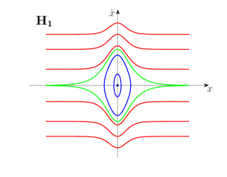
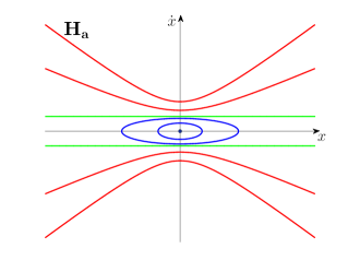
Figure 1: Phase portraits of H${}_{\text{\bf 1}}$ and H${}_{\text{\bf a}}$ systems.

In the case H${}_{\text{a}}$, as in the case H${}_{\text{1}}$ with $m=1$, coordinate $x$ can vary on all the real line, and trajectories in these two cases have a similar nature: they are bounded for energies $-1\leq E<0$, and unbounded for $E\geq 0$. It is interesting to note that the peculiarity of the case H${}_{\text{a}}$ is that all the phase space trajectories in it are conical sections. Namely, for $-1<E<0$ these are ellipses, $\frac{\dot{x}^{2}}{a^{2}}+\frac{x^{2}}{b^{2}}=1$ with $a^{2}=4(1+E)$, $b^{2}=(1+E)/(-E)$, which degenerate into a point $x=\dot{x}=0$ at $E=-1$. The case $E=0$ corresponds to sepatrices which here are straight lines $\dot{x}=\pm 2$, while for $E>0$ the trajectories are hyperbolas $\frac{\dot{x}^{2}}{a^{2}}-\frac{x^{2}}{b^{2}}=1$ with $a^{2}=4(1+E)$, $b^{2}=(1+E)/E$.

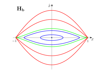
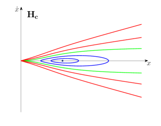
Figure 2: Phase portraits of H${}_{\text{\bf b}}$ and H${}_{\text{\bf c}}$ systems.

In the cases H${}_{\text{b}}$, H${}_{\text{d}}$ and H${}_{\text{e}}$ the variable $x$ varies in finite intervals, and phase space portraits in these cases have a similar nature. For $-1\leq E<0$ the trajectories are smooth curves lying between the extrema $x_{1}$ and $x_{2}$ of the corresponding intervals shown in Table 1, with returning points $x_{+}=-x_{-}$, $x_{1}<x_{-}<x_{+}<x_{2}$. For $E=0$ separatrices have cusps at $x_{1}$ and $x_{2}$, which reflect the fact that though the time necessary to arrive at these points is infinite, the derivative $d\dot{x}/dx$ at these points turns into zero. For $E>1$, the slopes $d\dot{x}/dx$ are finite at $x_{1,2}$ (and time to arrive at these points is infinite). The limiting points $x_{1,2}$ and the infinity of time necessary to arrive at them for trajectories with $E\geq 0$ are associated with poles of the position-dependent mass.

In the case H${}_{\text{c}}$, trajectories are bounded for $-1\leq E<0$, with returning points $x_{\pm}$, $0<x_{-}<x_{+}<\infty$. For $E=0$, separatrix has a cusp at $x=0$, and asymptotes $\dot{x}=\pm 4$ for $x\rightarrow+\infty$. For $E>0$, the trajectories are unbounded, with asymptotes given by $\frac{d\dot{x}}{dx}=\pm 2\sqrt{E}$ for $x\rightarrow+\infty$.

In the case H${}_{\text{b}}$, one can consider the infinite domains $x>1$ or $x<-1$ instead of the finite interval $x\in(-1,1)$, where the mass function also takes positive values. Let $x>1$, and denote this case as H${}^{\bf\prime}{}_{\text{\bf b}}$. Then $x=x(\chi)=-\coth\chi$, $\chi\in(-\infty,0)$, $x\in(1,\infty)$. In terms of $\chi$ (after the change of variable), we have a singular potential $U_{1}(\chi)=\frac{1}{\sinh^{2}\chi}$, and phase space trajectories with $E>0$ are unbounded, see Figure 3. The returning point $\chi_{0}$ is given by $\sinh\chi_{0}=-1/\sqrt{E}$, and asymptotes are $\dot{\chi}_{\pm}=\pm 2\sqrt{E}$. In coordinates ($x$, $\dot{x}$), however, trajectories are confined in the region $1<x\leq x_{0}$, $x_{0}^{2}=E+1$, where the returning point $x_{0}$ corresponds to the returning point $\chi_{0}$, while $x=1$ corresponds to the asymptotes with $\chi\rightarrow-\infty$, where we have $\frac{d\dot{x}}{dx}|_{x=1}=\pm 2\sqrt{E}$.

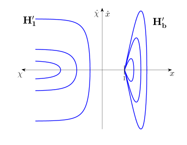
Figure 3: Phase portraits of H${{}^{\prime}}_{\text{1}}$ and H${{}^{\prime}}_{\text{b}}$ systems.

For position-dependent mass function we have $m(x)\rightarrow 0$ for $x\rightarrow x_{1,2}$ and unique maximum $m(0)=1$ in the case H${}_{\text{a}}$. On the other hand, $m(x)\rightarrow\infty$ for $x\rightarrow x_{1,2}$ in the cases H${}_{\text{b}}$, H${}_{\text{d}}$ and H${}_{\text{e}}$, with the unique minimum $m(0)=1$. In the case H${}_{\text{c}}$, the mass function changes monotonically: $m(x)\rightarrow\infty$ for $x\rightarrow x_{1}=0$ and $m(x)\rightarrow 0$ for $x\rightarrow x_{2}=\infty$.

4.3 Trigonometric family

Consider now the trigonometric T-family of the systems. Similarly to the H-family, Lagrangians for the systems presented in Table 2, $L=\frac{1}{4}m(x)\dot{x}^{2}-C_{n}u_{1}(x)$, can be obtained by starting from a particle with position-independent mass in two-dimensional Euclidean space and subjected to the action of repulsive Calogero potential, $L=\frac{1}{4}(\dot{X}^{2}+\dot{Y}^{2})-C_{n}\frac{1}{Y^{2}}$, and then restricting the motion to the semicircle $X^{2}+Y^{2}=1$, $Y>0$. Six different parametrizations of the semicircle $Y=\sqrt{1-X^{2}}$ given by the functions $X(x)$ and $Y(x)$ presented in Table 2 result in six models for finite-gap systems shown there. The mass function can be presented here as $m(x)=X^{\prime 2}/(1-X^{2})$, or $m(x)=Y^{\prime 2}/(1-Y^{2})$.

Table 2: T-family.
Corresponding finite-gap systems are given by potentials $u_{{}_{C_{n}}}(x)=C_{n}u_{1}(x)$ with $C_{n}=n(n+1)\hbar^{2}$, $n=1,2,\ldots$. Here $\chi\in(-\frac{\pi}{2},\frac{\pi}{2})$, $\text{gd}^{-1}\,x=\text{arctanh}\,(\sin x)$ is the inverse gudermannian function [58].

Case	$m(x)$	$\varphi(x)$	$x=x(\chi)$	$(x_{1},x_{2})$	$u_{1}(x)$	$X(x)$	$Y(x)$
T${}_{\text{1}}$	$1$	$1$	$\chi$	$(-\frac{\pi}{2},\frac{\pi}{2})$	$\frac{1}{\cos^{2}x}$	$\sin x$	$\cos x$
T${}_{\text{a}}$	$\frac{1}{1-x^{2}}$	$\cos\chi$	$\sin\chi$	(-$1,1$)	$\frac{1}{1-x^{2}}$	$x$	$\sqrt{1-x^{2}}$
T${}_{\text{b}}$	$\frac{1}{(1+x^{2})^{2}}$	$\frac{1}{\cos^{2}\chi}$	$\tan\chi$	$(-\infty,\infty)$	$x^{2}+1$	$\frac{x}{\sqrt{1+x^{2}}}$	$\frac{1}{\sqrt{1+x^{2}}}$
T${}_{\text{c}}$	$\frac{1}{e^{x}-1}$	$\frac{1+\sin\chi}{\cos\chi}$	$\ln\frac{2}{1-\sin\chi}$	$(0,\infty)$	$\frac{1}{4}\frac{e^{2x}}{e^{x}-1}$	$1-2e^{-x}$	$2\sqrt{e^{-x}-e^{-2x}}$
T${}_{\text{d}}$	$\frac{1}{\cosh^{2}x}$	$\frac{1}{\cos\chi}$	$\text{gd}^{-1}\,\chi$	$(-\infty,\infty)$	$\cosh^{2}x$	$\tanh x$	$\frac{1}{\cosh x}$
T${}_{\text{e}}$	$\text{dn}^{2}\,x$	$\frac{1}{\sqrt{1-k^{2}\sin^{2}\chi}}$	$\text{sn}^{-1}(\sin\chi)$	$(-\text{\bf K},\text{\bf K})$	$\text{nc}^{2}\,x$	$\text{sn}\,x$	$\text{cn}\,x$

As in the case of the H-family, the kinetic term for T-models can also be obtained by restricting the kinetic term of a particle on the Riemann sphere to some of its geodesics. Take the metric on the Riemann sphere in the form $ds^{2}=\frac{dX^{2}+dY^{2}}{(1+X^{2}+Y^{2})^{2}}$, $-\infty<X,Y<\infty$. Restricting the kinetic term $v^{2}\equiv(ds/dt)^{2}$ to the geodesic $X^{2}+Y^{2}=1$ parametrized by $X=\sin x$, $Y=\cos x$, we reproduce the kinetic term for T${}_{\text{1}}$ case with $m=1$. Restriction of $\frac{1}{4}v^{2}$ to the geodesic $Y=0$ with subsequent change of the notation $X\rightarrow x$ yields the kinetic term for T${}_{\text{b}}$ model. By appropriate change of the variable $x$, which can be found from the column $X(x)$ of the Table, one can reproduce all other kinetic terms for T-models.

The case T${}_{\text{e}}$ in the limits $k\rightarrow 0$ and $k\rightarrow 1$ transforms into the T${}_{\text{1}}$ and T${}_{\text{d}}$ cases, respectively. The family T${}_{\text{e}}$ can be considered therefore as that interpolating continuously between the position-independent mass, T${}_{\text{1}}$, and PDM, T${}_{\text{d}}$, cases of trigonometric finite-gap systems.

After the application of similarity transformation and the change of variable, we reduce all the cases to the corresponding quantum systems from the case T${}_{\text{1}}$. Such a system characterized by the integer parameter $n$ can be obtained by subsequent application of $n$ Darboux transformations to the free particle ($n=0$) confined into the infinite potential well with impenetrable walls at $\chi_{1}=-\frac{\pi}{2}$ and $\chi_{2}=\frac{\pi}{2}$ [53]. Energy levels of the bound states are $(n+l+1)^{2}-1$, $l=0,1,\ldots$. Though the Lax-Novikov integral can formally be obtained from hyperbolic case by the transformation $\chi\rightarrow i\chi$, this is a non-physical operator: its action on the physical states produces the states divergent at the edges $\chi_{1,2}=\pm\frac{\pi}{2}$ of the interval. The model T${}_{\text{1}}$ is often called in the literature the Higgs oscillator [69, 70, 71, 72, 73].

The phase portraits for T${}_{\text{1}}$, T${}_{\text{a}}$ and T${}_{\text{e}}$ cases are similar. All the trajectories with $E\geq 1$ in these cases, where $E=1$ corresponds to the minimum value of the potentials $u_{1}$, are bounded and closed, with returining points $x_{-}=-x_{+}$, $x_{1}<x_{-}<x_{+}<x_{2}$. There is, however, a difference between these cases: in the T${}_{\text{1}}$ case, the extrema points $x_{1,2}$ of the domain of $x$ correspond to singular points of the potential, while for T${}_{\text{a}}$ and T${}_{\text{e}}$ cases they correspond to zeros of the $1/m(x)$ function. The peculiarity of the T${}_{\text{a}}$ case is also that all the trajectories in it are ellipses: $\frac{\dot{x}^{2}}{a^{2}}+\frac{x^{2}}{b^{2}}=1$ with $a^{2}=4(E-1)$, $b^{2}=(E-1)/E$. This phase portrait is similar to that of the harmonic oscillator, with the difference that here $b^{2}$ is restricted from above, $b^{2}<1$, see Figure 4.

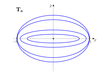
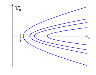
Figure 4: Phase portraits of T${}_{\text{\bf a}}$ and T${{}^{\prime}}_{\text{a}}$ systems.

In the case of T${}_{\text{c}}$, all the trajectories are closed, with returning points $x_{-}$ and $x_{+}$ satisfying the relation $0<x_{-}<x_{0}<x_{+}<\infty$, where $x_{0}=\ln 2$ corresponds to the point where potential takes the minimum value $1$, i.e., unlike the three above mentioned cases, here the values of the returning point $x_{+}$ are not bounded, see Figure 5. The phase portraits in $(x,\dot{x})$ coordinates for the cases T${}_{\text{b}}$ (note that in this case potential is quadratic) and T${}_{\text{d}}$ are similar to the phase portrait for a usual one-dimensional harmonic oscillator: the trajectories are closed smooth curves whose sizes increase with increasing of energy $E=\frac{1}{4}m(x)\dot{x}^{2}+u_{1}(x)$. There is, however, a difference in comparison with the harmonic oscillator. As it is seen from Figure 5, the trajectories in the T${}_{\text{b}}$ case are convex only for $1\leq E\leq E_{*}=\frac{3}{2}$, but they loose this property for $E>E_{*}$. In the case T${}_{\text{d}}$, $E_{*}=2$. Similar properties related to (non-)convexitivity of phase space trajectories is also characteristic of T${}_{\text{c}}$ case.

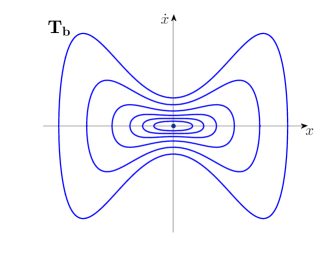
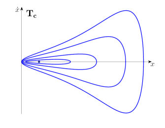
Figure 5: Phase portraits of T${}_{\text{\bf b}}$ and T${}_{\text{\bf c}}$ systems.

The model T${}_{\text{a}}$ can be modified for the case T${\bf{}^{\prime}}_{\text{\bf a}}$ with $x^{2}>1$ by multiplying Lagrangian by $-1$ to have a positive-valued mass function, $L=\frac{1}{4}\tilde{m}(x)\dot{x}^{2}-\tilde{u}_{1}(x)$, where $\tilde{m}(x)=\frac{1}{x^{2}-1}$, $\tilde{u}_{1}(x)=\frac{1}{x^{2}-1}$. In this case $x(\chi)=\cosh\chi$ with $\chi\in(0,\infty)$ and $x\in(1,\infty)$, and after the change of variable we obtain a singular Lagrangian $\tilde{U}_{1}(\chi)=\frac{1}{\sinh^{2}\chi}$ exactly as in the case T${\bf{}^{\prime}}_{\text{\bf b}}$. So, in coordinates $\chi$, $\dot{\chi}$ the unbounded trajectories for $E>0$ are exactly of the same form described above for the singular finite-gap model H${\bf{}^{\prime}}_{\text{\bf 1}}$ but with $\chi<-1$ there changed for $\chi>1$ in the case T${\bf{}^{\prime}}_{\text{\bf 1}}$ (we do not show these trajectories in coordinates $(\chi,\dot{\chi})$ here). Unlike the H${\bf{}^{\prime}}_{\text{\bf b}}$ model, here, in the T${\bf{}^{\prime}}_{\text{\bf a}}$ model, the trajectories are the hyperbolas $\frac{\dot{x}^{2}}{a^{2}}-\frac{x^{2}}{b^{2}}=-1$ with $a^{2}=4(1+E)$, $b^{2}=(1+E)/E$, $E>0$, see Figure 4.

In the case T${}_{\text{a}}$, function $m(x)$ tends to infinity when $x\rightarrow x_{1,2}$, taking minimum value $m(0)=1$. In the cases T${}_{\text{b}}$ and T${}_{\text{d}}$, $m(x)\rightarrow 0$ when $x\rightarrow x_{1,2}$, and takes maximum value $m(0)=1$. In the case T${}_{\text{e}}$, $m(x)\rightarrow k^{\prime 2}>0$ for $x\rightarrow x_{1,2}$, and takes maximum value $m(0)=1$. In the case T${}_{\text{c}}$, $m(x)$ changes monotinically, with $m(x)\rightarrow\infty$ when $x\rightarrow 0$ and $m(x)\rightarrow 0$ as $x\rightarrow\infty$.

4.4 Finite-gap elliptic L– and D–families

Consider now finite-gap elliptic generalizations of the hyperbolic and trigonometric families which are presented in Table 3. The phase portrait of the case L${}_{\text{1}}$, which is a periodic generalization of the H${}_{\text{1}}$ case, is shown in Figure 6.

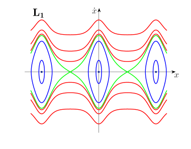
Figure 6: Phase portrait of L${}_{\text{1}}$ system with $k=0.99$.

Table 3: Elliptic L– and D–families.
Here $x_{{}_{E}}(\chi)=\frac{1}{k^{\prime}}\ln\left(1+k^{\prime}\frac{\text{dn}\,\chi+k^{\prime}\text{sn}\,\chi}{1-\text{sn}\,\chi}\right)$, $u_{{}_{L_{E}}}(x)=-k^{\prime 2}\left(\frac{e^{\xi}-k^{2}e^{-\xi}}{e^{\xi}+k^{2}e^{-\xi}-2k^{2}}\right)^{2}$, $u_{{}_{D_{E}}}(x)=\frac{1}{4}\frac{(e^{\xi}-k^{2}e^{-\xi})^{2}}{e^{\xi}+k^{2}e^{-\xi}-1-k^{2}}$, $\xi=k^{\prime}x$; $\text{am}\,\chi=\text{am}\,(\chi,k)=\text{Arcsin}\,\mathrm{sn}\,(\chi,k)$ is Jacobi’s amplitude function [57, 58]. The limiting cases H${}_{\alpha\,{\bf\pm}}$ are defined in the same way as H_α, $\alpha=$1,a,b,c,d, but with $u_{1}(x)$ changed for $u_{\pm}(x)=\pm 1$. Analogously, T${}_{\alpha\,-}$ is defined as T_α but with potential $u_{1}(x)$ changed for $u_{-}(x)=-1$.

Case	$m(x)$	$\varphi(\chi)$	$x=x(\chi)$		$u_{1}(x)$	$U_{1}(\chi)$	$k\rightarrow 1$	$k\rightarrow 0$
			$(\chi_{1},\chi_{2})$	$(x_{1},x_{2})$
L${}_{\text{1}}$	1	1	$\chi$		$-\text{dn}^{2}\,x$	$-\text{dn}^{2}\,\chi$	H${}_{\text{1}}$	H${}_{\text{1\,--}}$
			$(-\infty,\infty)$	$(-\infty,\infty)$
D${}_{\text{1}}$			(-K, K)	(-K, K)	$\text{dc}^{2}\,x$	$\text{dc}^{2}\,\chi$	H${}_{\text{1+}}$	T${}_{\text{1}}$
L${}_{\text{A}}$	$\frac{1}{(1-x^{2})(1-k^{2}x^{2})}$	$\text{cn}\,\chi\,\text{dn}\,\chi$			$k^{2}x^{2}-1$	$-\text{dn}^{2}\,\chi$	H${}_{\text{b}}$	T${}_{\text{a\,--}}$
			$\text{sn}\,\chi$
D${}_{\text{A}}$			(-K, K)	$(-1,1)$	$\frac{1-k^{2}x^{2}}{1-x^{2}}$	$\text{dc}^{2}\,\chi$	H${}_{\text{b+}}$	T${}_{\text{a}}$
L${}_{\text{B}}$	$\frac{1}{(1+x^{2})(1+k^{\prime 2}x^{2})}$	$\text{dn}\,\chi\,\text{nc}^{2}\,\chi$			$-\frac{1+k^{\prime 2}x^{2}}{1+x^{2}}$	$-\text{dn}^{2}\,\chi$	H${}_{\text{a}}$	T${}_{\text{b\,--}}$
			$\text{sc}\,\chi$
D${}_{\text{B}}$			(-K, K)	$(-\infty,\infty)$	$k^{\prime 2}x^{2}+1$	$\text{dc}^{2}\,\chi$	H${}_{\text{a+}}$	T${}_{\text{b}}$
L${}_{\text{C}}$	$\frac{1}{1-k^{2}\sin^{2}x}$	$\text{dn}\,\chi$	$\text{am}\,\chi$		$k^{2}\sin^{2}x-1$	$-\text{dn}^{2}\,\chi$	H${}_{\text{d}}$	H${}_{\text{1\,--}}$
			$(-\infty,\infty)$	$(-\infty,\infty)$
D${}_{\text{C}}$			(-K, K)	(-$\frac{\pi}{2}$, $\frac{\pi}{2}$)	$\frac{1-k^{2}\sin^{2}x}{\cos^{2}x}$	$\text{dc}^{2}\,\chi$	H${}_{\text{d+}}$	T${}_{\text{1}}$
L${}_{\text{D}}$	$\frac{1}{1+k^{\prime 2}\sinh^{2}x}$	$\text{dc}\,\chi$			$-k^{\prime 2}-\frac{k^{2}}{\cosh^{2}x}$	$-\text{dn}^{2}\,\chi$	H${}_{\text{1}}$	T${}_{\text{d\,--}}$
			$\text{arcsinh}\,(\text{sc}\,\chi)$
D${}_{\text{D}}$			(-K, K)	$(-\infty,\infty)$	$k^{\prime 2}\sinh^{2}x+1$	$\text{dc}^{2}\,\chi$	H${}_{\text{1+}}$	T${}_{\text{d}}$
L${}_{\text{E}}$	$\frac{k^{\prime 2}}{(1-e^{-\xi})(e^{\xi}-k^{2})}$	$\text{nc}\,\chi+\text{sc}\,\chi$			$u_{{}_{L_{E}}}(x)$	$-\text{dn}^{2}\,\chi$	H${}_{\text{c}}$	T${}_{\text{c\,--}}$
			$x_{{}_{E}}(\chi)$
D${}_{\text{E}}$			(-K, K)	$(0,\infty)$	$u_{{}_{D_{E}}}(x)$	$\text{dc}^{2}\,\chi$	H${}_{\text{c+}}$	T${}_{\text{c}}$

The L${}_{\text{E}}$ and D${}_{\text{E}}$ cases can be considered as a generalization of the cases H${}_{\text{c}}$ and T${}_{\text{c}}$. To see this we note that the function $\varphi_{{}_{E}}(\chi)=(1+\mathrm{sn}\,\chi)/{\mathrm{cn}\,\chi}$ transforms in the limits $k\rightarrow 1$ and $k\rightarrow 0$ into the functions $\varphi(\chi)$ of the indicated hyperbolic and trigonometric cases. By means of (3.4) we find $x_{{}_{E}}(\chi)=\frac{1}{k^{\prime}}\ln\left(1+k^{\prime}\frac{\text{dn}\,\chi+k^{\prime}\text{sn}\,\chi}{1-\text{sn}\,\chi}\right),$ and then $\mathrm{sn}\,\chi=1-{2k^{\prime 2}}({e^{\xi}-2k^{2}+k^{2}e^{-\xi}})^{-1},$ $\xi=k^{\prime}x\,.$ This allows us to identify the potentials $u_{{}_{L_{E}}}(x)$ and $u_{{}_{D_{E}}}(x)$ using the indentities $\text{dn}^{2}\chi=1-k^{2}\text{sn}^{2}\,\chi$ and $\text{cn}^{2}\,\chi=1-\text{sn}^{2}\,\chi$. For $f(x)=\varphi(\chi)|_{\chi=\chi(x)}$, we obtain $f(x)=\frac{1}{k^{\prime}}\sqrt{(1-e^{-\xi})(e^{\xi}-k^{2})},$ and finally find the corresponding position dependent mass shown in the Table 3. The potentials $u_{{}_{L_{E}}}(x)$ and $u_{{}_{D_{E}}}(x)$ can be presented equivalently as

$$u_{{}_{L_{E}}}(x)=-k^{\prime 2}\frac{\sinh^{2}\xi_{k}}{(\cosh\xi_{k}-k)^{2}}\,,\qquad u_{{}_{D_{E}}}(x)=k^{2}\frac{\sinh^{2}(\xi_{k})}{2k(\cosh\xi_{k}-k)-k^{\prime 2}}\,,$$ (4.8)

where $\xi_{k}\equiv\xi-\ln k$.

Jacobi’s amplitude function $\text{am}\,(x,k)$ satisfies relations $\text{am}(x,0)=x$, $\text{am}\,(x,1)=\text{gd}\,x$, and can be considered as a generalization of the gudermannian function. In correspondence with this we note that $x=x(\chi)=\text{am}\,\chi$, which is the change of variable function in the case L${}_{\text{C}}$, appears as a generalization of the kink solution in the sine-Gordon model [74, 75].

In the case A, the even mass function $m(x)$ takes minimum value $m(0)=1$ and $m(x)\rightarrow\infty$ for $x\rightarrow\pm 1$. In the cases B and D, even mass function takes maximum value $m(0)=1$ and $m(x)\rightarrow 0$ for $x\rightarrow\pm\infty$. In the case C, $m(-x)=m(x)$, $m(0)=1$ and $m\rightarrow 1/k^{\prime 2}$ for $x\rightarrow\pm\frac{\pi}{2}$.

In correspondence with the behaviour of $U_{1}(\chi)=\text{dc}^{2}\,\chi$, potential $u_{1}(x)$ in all the cases of the D-family tends to $+\infty$ when $x$ tends to the corresponding edge values $x_{1,2}$, taking minimum value $+1$ at $x=0$ in all the cases except the case D${}_{\text{E}}$, where this happens at $x=\frac{1}{k^{\prime}}(\ln k+\text{arccosh}\,\frac{1}{k})$, that is the root of the equation $\cosh\xi_{k}=\frac{1}{k}$. Analogously, in correspondence with $U_{1}(\chi)=-\text{dn}^{2}\,\chi$, potential $u_{1}(x)$ in the cases of the L-family tends to the maximum value $-k^{\prime 2}$ when $x\rightarrow x_{1,2}$, taking minimum value $-1$ at $x=0$ in all the cases except the case L${}_{\text{E}}$, where this minimum value is taken at $x=\frac{1}{k^{\prime}}\ln(1+k^{\prime})$.

From the two last columns of the Table 3 we also see that elliptic (after similarity transformation and the change of variable) Lamé models L provide us with some interpolation between reflectionless models H and corresponding free particle models with position-dependent, or position-independent (unit) mass function. Particularly, the case L${}_{\text{B}}$ provides a finite-gap periodic generalization of the Mathews-Lakshmanan oscillator model described by the case H${}_{\text{a}}$, while the L${}_{\text{A}}$ case can be considered as a finite-gap periodic generalization of the ‘inflationary model’ H${}_{\text{b}}$. Analogous job is made by the Darboux-Treibich-Verdier models D, which can be considered as the systems interpolating between the trigonometric models T and corresponding free particle systems.

We do not discuss the spectrum and corresponding Lax-Novikov operators of finite-gap systems of the L– and D–families here, and just refer to [54, 76].

In conclusion of this subsection, it is worth to make an additional comment here to be valid for each of the three families of finite-gap systems presented above. If after corresponding similarity transformations and changes of variables two systems with different position dependent masses $m(x)$ and $\tilde{m}(\xi)$ and potentials $u(x)$ and $\tilde{u}(\xi)$ produce the same system $H=-\frac{d^{2}}{d\chi^{2}}+U(\chi)$, the following equality for the quantum kinetic terms has to be valid: $\sqrt{f}\left(\sqrt{f}\frac{d}{dx}\sqrt{f}\right)^{2}\frac{1}{\sqrt{f}}|_{x=x(\chi)}=\sqrt{\tilde{f}}\left(\sqrt{\tilde{f}}\frac{d}{d\xi}\sqrt{\tilde{f}}\right)^{2}\frac{1}{\sqrt{\tilde{f}}}|_{\xi=\xi(\chi)}$. From this equality we find that to establish the relation between the quantum kinetic terms of any two systems presented in the tables which produce the same quantum system $H=-\frac{d^{2}}{d\chi^{2}}+U(\chi)$, the following additional similarity transformation is required:

$$\left(\sqrt{f(x)}\frac{d}{dx}\sqrt{f(x)}\right)^{2}=\sqrt{\frac{\tilde{f}(\xi)}{f(x)}}\left(\sqrt{\tilde{f}(\xi)}\frac{d}{d\xi}\sqrt{\tilde{f}(\xi)}\right)^{2}\sqrt{\frac{f(x)}{\tilde{f}(\xi)}}|_{\xi=\xi(x)}\,.$$ (4.9)

Here, on the right hand side of Eq. (4.9), $\xi=\xi(x)$ is given by $\xi(x)=\xi(\chi)|_{\chi=\chi(x)}$, and so, $\tilde{u}(\xi(x))=u(x)$. For example, the system from the elliptic case A can be obtained from the corresponding systems of the elliptic case C by the changes of variables $x\rightarrow\xi$, $\xi=\sin x$. In this way the potentials $u(x)$ from the case C transform into corresponding potentials of the case A. For kinetic term we have then $\left(\sqrt{f_{\text{\bf C}}}\frac{d}{dx}\sqrt{f_{\text{\bf C}}}\right)^{2}\rightarrow(1-x^{2})^{1/4}\left(\sqrt{f_{\text{\bf A}}}\frac{d}{dx}\sqrt{f_{\text{\bf A}}}\right)^{2}(1-x^{2})^{-1/4}$. Thus after additional similarity transformation quantum Hamiltonian $H_{\text{\bf C}}(x)$ transforms into $H_{\text{\bf A}}(x)$.

4.5 Elliptic finite-gap systems and Seiffert’s spiral

The systems presented in Table 3 can be obtained from a particle on the unit sphere subjected to the action of certain potentials of the forms like those indicated at the beginning of the section, to which it is necessary to apply a certain reduction procedure. To show this we take the $\mathbb{R}^{3}$ metric in cylindrical coordinates $ds^{2}=\rho^{2}d\phi^{2}+d\rho^{2}+dz^{2}$. On the surface of the unit sphere this can be reduced to one of the two forms

$$ds^{2}(z,\phi)=(1-z^{2})d\phi^{2}+\frac{dz^{2}}{1-z^{2}},\qquad ds^{2}(\rho,\phi)=\rho^{2}d\phi^{2}+\frac{dz^{2}}{1-\rho^{2}}\,,$$ (4.10)

where we have used the sphere equation $\rho^{2}+z^{2}=1$ to eliminate the dependence on $\rho$ or $z$. Let us restrict additionally the motion by requiring that $d\phi=kds$, where $k\in\mathbb{R}$ is a constant. As a result, $L_{0}=\frac{1}{4}(ds/dt)^{2}$ takes the form of the kinetic term for a particle moving along the Seiffert’s spiral [57, 77]. Particularly, if we take $z=\pm\frac{1}{\sqrt{1-x^{2}}}$, $x\in[-1,1]$, that corresponds to the function $Y(x)$ from T${}_{\text{b}}$ case but with a sign, and use the first form $ds^{2}(z,\phi)$ from (4.10), we reproduce the mass term for L${}_{\text{A}}$ and D${}_{\text{A}}$ cases. Potential can be chosen initially in the Calogero-like form $u_{1}(z)=-k^{\prime 2}-\frac{k^{2}}{z^{2}}$ for L families, or in the harmonic oscillator form $u_{1}(z)=k^{\prime 2}z^{2}+k^{2}$ for D families. The same L${}_{\text{A}}$ and D${}_{\text{A}}$ systems can be reproduced by using $ds^{2}(\rho,\phi)$, and setting $\rho=x$ which corresponds to $X(x)$ from the same T${}_{\text{b}}$ case . The initial form of potentials is interchanged in comparison with the case when we proceed from the $ds^{2}(z,\phi)$ form of the spherical metric: we should take $u_{1}(\rho)=-k^{\prime 2}-\frac{k^{2}}{\rho^{2}}$ for the D case and $u_{1}(\rho)=k^{\prime 2}\rho^{2}+k^{2}$ for the L case. In the same vein one can use other parametrizations for $z$ and $\rho$ coordinates shown in Table 2 to reproduce the systems presented in Table 3. The correspondence between parametrizations and elliptic families is the following: T${}_{\text{e}}$ $\rightarrow$ 1, T${}_{\text{b}}$ $\rightarrow$ B, T${}_{\text{1}}$ $\rightarrow$ C, T${}_{\text{d}}$ $\rightarrow$ D. At the same time, if we take $\rho=\pm(1-2e^{-x})$ corresponding to a parametrization from the case T${}_{\text{c}}$, we do not reproduce the last case E, but obtain, instead, $L_{0}=\frac{1}{4}m(x)\dot{x}^{2}$ with position-dependent mass $m(x)$ and $x(\chi)$ functions given by

$$m(x)=\frac{1}{(e^{x}-1)k^{\prime 2}+4k^{2}(1-e^{-x})^{2}}\,,\qquad x(\chi)=-\ln\left(\frac{1}{2}(1+\mathrm{sn}\,\chi)\right)\,,$$ (4.11)

and potentials

$$u_{1}(x)=4k^{2}(e^{-2x}-e^{-x})-k^{\prime 2}\,,\qquad u_{1}(x)=\frac{k^{\prime 2}+4k^{2}(e^{-x}-e^{-2x})}{4(e^{-2x}-e^{-x})}\,$$ (4.12)

for the cases L${}_{\text{E}}$ and D${}_{\text{E}}$, respectively. In the limit $k\rightarrow 0$, the mass function from (4.11) transforms into that for the case T${}_{\text{c}}$, but for $k\rightarrow 1$ we obtain $m(x)=\frac{1}{4(1-e^{-x})^{2}}$, which does not appear in Table 3, and, particularly, does not coincide with $m(x)$ for the H${}_{\text{c}}$ case. There is no contradiction here since in general different elliptic functions may have the same limit for $k\rightarrow 0$ (or for $k\rightarrow 1$), but different limits as $k\rightarrow 1$ ($k\rightarrow 0$). For the discussion of this point in application to finite-gap systems, see [54, 55, 56].

The first function from (4.12) has a form of Morse potential. So, the system (4.11) with first potential from (4.12) gives us finite-gap elliptic generalization of reflectionless system with position-dependent mass $m(x)=\frac{1}{4(1-e^{-x})^{2}}$ and Morse-like potential $u_{1}(x)=4(e^{-2x}-e^{-x})$.

4.6 Special case of elliptic finite-gap systems and Bernoulli lemniscate

In the limits $k\rightarrow 1$ and $k\rightarrow 0$, the elliptic finite-gap systems we considered transform into hyperbolic and trigonometric systems. A rather natural question that appears here whether anything interesting happens in the middle case, at $k^{2}=k^{\prime 2}=\frac{1}{2}$ . In this case we have $k=k^{\prime}=\frac{1}{\sqrt{2}}$, and so, $\text{\bf K}(k)=\text{\bf K}(k^{\prime})\equiv\text{\bf K}^{\prime}(k)$, i.e. in this case the magnitudes of the real, $2\text{\bf K}(1/\sqrt{2})$ and the hidden imaginary, $2i\text{\bf K}^{\prime}(1/\sqrt{2})$, periods of finite-gap L– and D–potentials $-C_{n}\,\mathrm{dn}^{2}\,\chi$ and $C_{n}\,\text{dc}^{2}\,\chi$ coincide. This corresponds to the lemniscatic case of elliptic functions [57, 58] with a purely imaginary value $k=i$ of the modular parameter for which $\mathrm{sn}\,(z,i)=\frac{1}{\sqrt{2}}\,\mathrm{sd}\,\left(\sqrt{2}\,z,{1}/{\sqrt{2}}\right)$, $\mathrm{cn}\,(z,i)=\mathrm{cd}\,\left(\sqrt{2}\,z,{1}/{\sqrt{2}}\right)$ and $\mathrm{dn}\,(z,i)=\mathrm{nd}\,\left(\sqrt{2}\,z,{1}/{\sqrt{2}}\right)$, see Appendix B. In the case $k=i$ for the complementary modular parameter we have $k^{\prime 2}=1-k^{2}=2$.

In lemniscatic case $k=i$, the Hamiltonian operator of finite-gap Lamé system takes the form $H^{\text{\bf L}}_{n}=2\left(-\frac{d^{2}}{d\zeta^{2}}-C_{n}\mathrm{dn}^{2}\,(\zeta,1/\sqrt{2}\right)$, where $\zeta\equiv\sqrt{2}\,\chi+\text{\bf K}\left({1}/{\sqrt{2}}\right)$. This is just the rescaled Hamiltonian of the displaced in a half-period $n$-gap Lamé system with $k=1/\sqrt{2}$.

For the basic D–potential with $k=i$ we have $\text{dc}^{2}\,(\chi,i)=\text{nc}^{2}(\sqrt{2}\,\chi,1/\sqrt{2})=-2\mathrm{dn}^{2}\,(\zeta,1/\sqrt{2})+1$, $\zeta\equiv\sqrt{2}\,\chi+\text{\bf K}(1/\sqrt{2})+i\text{\bf K}^{\prime}(1/\sqrt{2}))$, and the Hamiltonian is rewritten equivalently $H_{n}^{\text{\bf D}}=2\left(-\frac{d^{2}}{d\zeta^{2}}-C_{n}\mathrm{dn}^{2}\,(\zeta,1/\sqrt{2})\right)+1$. This is a rescaled finite-gap D-Hamiltonian operator.

Let us show now that all the L- and D- finite-gap systems with position-dependent mass presented in Table 3, in the lemniscatic case $k=i$ can be obtained from a non-relativistic particle of mass $m=1$ in Eucledian space $\mathbb{R}^{2}$ with coordinates $(\xi,\eta)$, which is subjected to the action of one of the two basic potentials

$$u^{\text{\bf L}}_{1}(\xi,\eta)=-\frac{2}{\xi^{2}+\eta^{2}+1}\,,\qquad u^{\text{\bf D}}_{1}(\xi,\eta)=\frac{1}{\xi^{2}+\eta^{2}}\,$$ (4.13)

and restricted to move along the Bernoulli lemniscate.

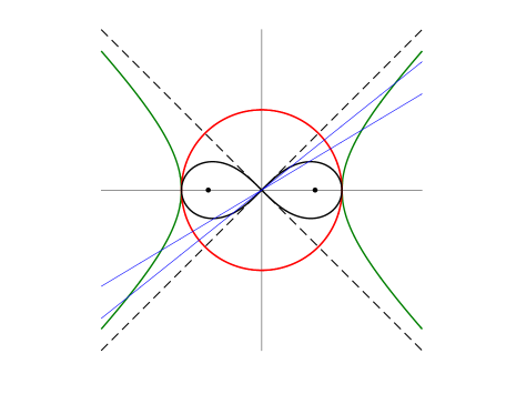
Figure 7: Bernoulli lemniscate, equilateral hyperbola and circumference of inversion.

Bernoulli lemniscate can be obtained in the following way directly relevant to our consideration. Take an equilateral (rectangular) hyperbola in Euclidean $\mathbb{R}^{2}$ space given by the equation $X^{2}-Y^{2}=1$, and construct its inversion in the circle of unit radius centered at the origin of the system of coordinates, see Figure 7. We obtain $(X,Y)\longmapsto(\xi,\eta)\,,$ where

$$(\xi,\eta)=\left(\frac{X}{X^{2}+Y^{2}}\,,\,\frac{Y}{X^{2}+Y^{2}}\right)\,.$$ (4.14)

We have $\xi^{2}+\eta^{2}=1/(X^{2}+Y^{2})$, $\xi^{2}-\eta^{2}=1/(X^{2}+Y^{2})^{2}$, and so, the points of the inverted hyperbola satisfy the equation

$$(\xi^{2}+\eta^{2})^{2}=\xi^{2}-\eta^{2}\,.$$

This is nothing else as the equation of a particular case of the Bernoulli lemniscate $(\xi^{2}+\eta^{2})^{2}=2c^{2}(\xi^{2}-\eta^{2})$ with foci at $(-c,0)$ $(+c,0)$ with $c=1/\sqrt{2}$, and unit ‘radius’ $\sqrt{2}\,c=1$.

For a particle restricted to move on the lemniscate, we have

$$\dot{\xi}^{2}+\dot{\eta}^{2}=\frac{\dot{Y}^{2}}{(1+Y^{2})(1+2Y^{2})}\,,$$ (4.15)

where we have taken into account that $X^{2}-Y^{2}=1$. Taking now all the different parametrizations for the equilateral hyperbola presented in Table 1 (with the change $X\leftrightarrow Y$), we reproduce all the finite-gap elliptic systems with $k=i$ presented in Table 3. The correspondence between the parametrization cases and elliptic (lemniscatic) families is the following:

$$\text{\bf H}{}_{\text{\bf 1}}\rightarrow\text{\bf D},\qquad\text{\bf H}{}_{\text{\bf a}}\rightarrow\text{\bf B},\qquad\text{\bf H}{}_{\text{\bf b}}\rightarrow\text{\bf A},\qquad\text{\bf H}{}_{\text{\bf c}}\rightarrow\text{\bf E},\qquad\text{\bf H{}}_{\text{\bf d}}\rightarrow\text{\bf C},\qquad\text{\bf H{}}_{\text{\bf e}}\rightarrow\text{\bf 1}\,.$$ (4.16)

For instance, using the parametrization from the case $\text{\bf H}{}_{\text{\bf 1}}$, we put $Y=\sinh x$, and (4.15) gives us the kinetic term $L_{0}=\frac{1}{4}m(x)\dot{x}^{2}$ with $m(x)=1/(1+2\sinh^{2}x)$, that coincides with the position-dependent mass from Table 3 for the D family in the lemniscatic case $k=i$. Potentials (4.13) take here the form of the potentials of the lemniscatic D family: $u^{\text{\bf L}_{\bf D}}_{1}=-2+\cosh^{2}x$ and $u^{\text{\bf D}_{\bf D}}_{1}=1+2\sinh^{2}x$. Using the parametrization for the case $\text{\bf H}{}_{\text{\bf e}}$, we put $Y=\frac{\mathrm{sn}\,(x,k)}{\mathrm{cn}\,(x,k)}$, and (4.15) gives us $m(x)=\mathrm{dn}^{2}\,(x,k)/(1+\mathrm{sn}^{2}\,(x,k))$. For lemniscatic case $k=i$ this reduces to the constant mass $m=1$ for the family 1 from Table 3, while (4.13) gives us the corresponding potentials. In a similar way, one can check other correspondences shown in Eq. (4.16). Particularly, parametrization $Y=\frac{x}{\sqrt{1-x^{2}}}$ from $\text{\bf H}{}_{\text{\bf b}}$ case gives the mass function $m(x)=\frac{1}{1-x^{4}}$ of the lemniscatic case for the family A. Since for $\text{\bf H}{}_{\text{\bf a}}$ case we have $Y=x$, Eq. (4.15) gives us immediately the mass function for the lemniscatic B family: $m(x)=\frac{1}{(1+x^{2})(1+2x^{2})}$. The only correspondence that requires an additional step to establish is $\text{\bf H}{}_{\text{\bf c}}\rightarrow\text{\bf E}$. The parametrization from the case $\text{\bf H}{}_{\text{\bf c}}$ with $X=\frac{1}{2}(\kappa+\frac{1}{\kappa})$, $Y=\frac{1}{2}(\kappa-\frac{1}{\kappa})$ gives us the rational parametrization (4.14) of the lemniscate,

$$(\xi,\eta)=\left(\frac{\kappa^{3}+\kappa}{\kappa^{4}+1},\frac{\kappa^{3}-\kappa}{\kappa^{4}+1}\right),$$

and the kinetic term $L_{0}(\kappa)=\frac{1}{4}m(\kappa)\dot{\kappa}^{2}$ with the position-dependent mass $m(\kappa)=2/(1+\kappa^{4})$. Changing additionally the parameter by $\kappa=\sqrt{\sinh\tau}$, $\tau\equiv\sqrt{2}\,x$, where we assume $x>0$, the obtained kinetic term transforms into $L_{0}(x)=\frac{1}{4}m(x)\dot{x}^{2}$ with $m(x)=\frac{1}{\sinh\tau}$, that corresponds to the lemniscatic case $k=i$ of the position-dependent mass for the finite-gap family E from the Table 3. It is not difficult to check also that Eq. (4.13) reproduces correctly the lemniscatic form of the potentials for the same family E.

4.7 Finite-gap systems by reduction of a free particle on surfaces of revolution

We have showed how hyperbolic, trigonometric and elliptic finite-gap systems with PDM can be obtained by appropriate reduction procedures in different spaces of constant curvature in the presence of Calogero-like or harmonic oscillator potentials, or potentials related to these ones via appropriate coordinate transformations. Here we discuss how the same systems can be generated by the angular momentum reduction of a free particle system on some surfaces of revolution.

Hyperbolic finite-gap systems can be obtained by taking a free non-relativistic particle on one-sheet hyperboloid embedded into (2+1)-dimensional Minkowski space $\mathbb{R}^{1,2}$, the $AdS_{2}$ space, and by making a phase space reduction of the system to a surface of a constant angular momentum. Indeed, consider a one-sheet hyperboloid with coordinates $x^{0}=X(x)$, $\vec{x}=Y(x)\vec{n}(\varphi)$, where $Y(x)=\sqrt{1+X^{2}(x)}$, $-\infty<X(x)<\infty$, $\vec{n}(\varphi)=(\cos\varphi,\sin\varphi)$, $0\leq\varphi<2\pi$. We assume the hyperboloid is imbedded into the (2+1)-dimensional Minkowski space with metric $\eta_{\mu\nu}=\text{diag}\,(+1,-1,-1)$. From a free particle Lagrangian $L=\frac{1}{4}\eta_{\mu\nu}\dot{x}^{\mu}\dot{x}^{\nu}=\frac{1}{4}((\dot{x}^{0})^{2}-(\dot{\vec{x}})^{2})$ in $\mathbb{R}^{1,2}$ we obtain the Lagrangian $L=\frac{1}{4}(m(x)\dot{x}^{2}-Y^{2}(x)\dot{\varphi}^{2})$, where $m(x)=X^{\prime 2}/(1+X^{2})=Y^{\prime 2}/(Y^{2}-1)$. By the construction, the system is $SO(2,1)$-invariant. The angular coordinate $\varphi$ is cyclic, and corresponding Routhian is $R=\frac{1}{4}\left(m(x)\dot{x}^{2}-p_{\varphi}^{2}\frac{1}{Y^{2}(x)}\right)$. Conserved canonical momentum $p_{\varphi}=-\frac{1}{2}Y^{2}(x)\dot{\varphi}$ is the angular momentum of the system generating rotations in the plane $\vec{x}\in\mathbb{R}^{2}$, and reduction of the system to the surface $p_{\varphi}=C$ corresponds to the Lagrangian $L=\frac{1}{4}\left(m(x)\dot{x}^{2}-C^{2}\frac{1}{Y^{2}}\right)$ considered by us when we started our discussion of the hyperbolic family of the systems. On the other hand, the reduction can be realized at the quantum level in such a way that the quantum constant $C_{n}=n(n+1)\hbar^{2}$ will be reproduced exactly in the emerging potential term. For this it is necessary to introduce into initial Lagrangian a topologically nontrivial term $-\alpha\dot{\varphi}$, which does not change classical equations of motion and corresponds to coupling of the particle to the Aharonov-Bohm flux [68].

In analogous way, one can obtain trigonometric finite-gap systems by considering a free particle on a sphere embedded in 3D Euclidean space, $x_{3}=X(x)$, $\vec{x}=Y(x)=\vec{n}(\varphi)$, where $X^{2}+Y^{2}=1$, $Y>0$, and $\vec{n}(\varphi)$ is the unit vector as in the hyperbolic case. Then $L=\frac{1}{4}(\dot{x}^{3})^{2}+(\dot{\vec{x}})^{2}=\frac{1}{4}\left(m(x)\dot{x}^{2}+Y^{2}(x)\dot{\varphi}^{2}\right)$, $m(x)=\frac{Y^{\prime 2}}{1-Y^{2}}$. Analogously to the previous hyperbolic case, by reduction to the surface of the constant angular momentum $p_{\varphi}$ one can reproduce finite-gap trigonometric systems.

One can also consider a free motion of the particle on upper (or lower) sheet of the two-sheeted hyperboloid $(x^{0})^{2}-(\vec{x})^{2}=1$ embedded into the three-dimensional Minkowski space  $\mathbb{R}^{2,1}$. Taking the upper sheet given by $x^{0}=X(x)=\sqrt{1+Y^{2}(x)}$, $\vec{x}=Y(x)\vec{n}(\varphi)$ and a free particle Lagrangian in the form $L=\frac{1}{4}((\dot{\vec{x}})^{2}-(\dot{x}^{0})^{2})$, we obtain $L=\frac{1}{4}m(x)\dot{x}^{2}+Y^{2}(x)\dot{\varphi}^{2}$ and $R=\frac{1}{4}m(x)\dot{x}^{2}+p_{\varphi}^{2}\frac{1}{Y^{2}(x)}$, $m(x)=\frac{Y^{\prime}{}^{2}}{1+Y^{2}}$. After reduction to the surface $p_{\varphi}=C$ of a constant value of the integral of motion $p_{\varphi}$, one can reproduce singular finite-gap hyperbolic systems. Particularly, the choice $Y(x)=\frac{1}{\sqrt{x^{2}-1}}$, $x>1$, reproduces the system H${{}{\bf{}^{\prime}}}_{\text{\bf b}}$ with $m(x)=\frac{1}{(x^{2}-1)^{2}}$ and $u_{1}(x)=x^{2}-1$, which after the change of variable $x\rightarrow\chi$, $x=-\coth\chi$, $\chi<0$, transforms this into the system H${{}{\bf{}^{\prime}}}_{\text{\bf 1}}$ with $m=1$ and $U_{1}(\chi)=\frac{1}{\sinh^{2}\chi}$. The choice $Y(x)=\sqrt{x^{2}-1}$, $x>1$, reproduces the system T${{}{\bf{}^{\prime}}}_{\text{\bf a}}$ with $m(x)=\frac{1}{x^{2}-1}=u_{1}(x)$, which after the change of variable gives $m(\chi)=1$ and $U_{1}(\chi)=\frac{1}{\sinh^{2}\chi}$.

The both hyperbolic reflectionless H and finite-gap singular H^′ families can be obtained from ordinary Lorentzian anti-De Sitter spacetime $AdS_{3}$ of curvature radius $\ell$ by treating it as being embedded in $\mathbb{R}^{2,2}$. The embedding is given by the equation $-(\vec{x}_{-})^{2}+(\vec{x}_{+})^{2}=-\ell^{2}$, where $\vec{x}_{\pm}$ are two-dimensional vectors with components which we denote by $x^{1,2}_{\pm}$. Parametrization $\vec{x}_{-}=\ell\cosh\rho\,\vec{n}_{-}(\tau/\ell)$, $\vec{x}_{+}=\ell\sinh\rho\,\vec{n}_{+}(\varphi)$, $\vec{n}_{\pm}=(\cos\lambda_{\pm},\sin\lambda_{\pm})$, $\varphi\in[0,2\pi)$, $\tau\in[0,2\pi\ell)$, $\rho\in[0,\infty)$ gives the $AdS_{3}$ metric

$$ds^{2}=-\cosh^{2}\rho\,d\tau^{2}+\ell^{2}\sinh^{2}\rho\,d\varphi^{2}+\ell^{2}d\rho^{2}\,.$$ (4.17)

Taking a free particle in $AdS_{3}$ described by Lagrangian $L_{0}=\frac{1}{4}(ds/dt)^{2}=\frac{1}{4}(-\cosh^{2}\rho\,\dot{\tau}^{2}+\ell^{2}\sinh^{2}\rho\,\dot{\varphi}^{2}+\ell^{2}\dot{\rho}^{2})$, the Hamiltonian reduction by constraints $p_{\varphi}=C_{1}$, $p_{\tau}=0$ provides us with singular finite-gap systems H${}_{\bf 1}^{\prime}$. Instead of the second condition (constraint) one can take $\tau=0$, that corresponds to restriction on the subspace $x^{2}_{-}=0$, $x^{1}_{-}\geq\ell$. To obtain the reflectionless H₁-family, we reduce the system by using the constraints $p_{\tau}=C$, $x^{2}_{+}=0$. In the subspace with $x^{2}_{+}=0$ we have $x^{1}_{+}\geq 0$ that corresponds to $\varphi=0$, and $x^{1}_{+}\leq 0$ for $\varphi=\pi$. These two subspaces can be unified by taking $\varphi=0$ and extending $\rho$ from $[0,\infty)$ to the infinite interval $(-\infty,\infty)$. Such extension (doubling) of the interval for the variable $\rho$ is similar to the picture taking place for the motion along the Seiffert spiral we utilized to generate finite-gap elliptic systems. Again, by appropriate change of the variable $\rho$, we reproduce all the hyperbolic finite-gap systems with position-dependent mass we discussed.

One can also obtain elliptic systems L by taking a free particle on a certain surface of revolution embedded into Minkowski (2+1)-dimensional space. For the family $\text{\bf L}{}_{\text{\bf 1}}$, the corresponding surface in a two-parametric form is given by $x^{0}=\frac{1}{k^{\prime}}\text{E}(\xi,k)$, $\vec{x}=\frac{1}{\mathrm{dn}\,\chi}\vec{n}(\varphi)$, where $\xi=k^{\prime}\text{sc}\,(\chi,k)=-\mathrm{cn}\,(\chi+\text{\bf K},k)$, and $\text{E}(\xi,k)$ is the incomplete elliptic integral of the second kind, $\text{E}(x,k)=\int_{0}^{x}\sqrt{\frac{1-k^{2}\tau^{2}}{1-\tau^{2}}}d\tau$. This surface represents a surface of a form of a one-sheet hyperboloid but with $-\text{\bf E}\leq x^{0}\leq\text{\bf E}$, where $\text{\bf E}=\text{E}(1,k)$ is the complete elliptic integral of the second kind [57]. In the limit $k\rightarrow 1$, this surface transforms into the one-sheeted hyperboloid ($AdS_{2}$) surface we discussed above, while in the another limit $k\rightarrow 0$, it transforms into a cylinder with $-\pi\leq x^{0}\leq\pi$. We have here $L_{0}=\frac{1}{4}((\dot{x}^{0})^{2}-(\dot{\vec{x}})^{2})=\frac{1}{4}(\dot{\chi}^{2}-\mathrm{nd}^{2}\,\chi\,\dot{\varphi}^{2})$. After reduction to the surface $p_{\varphi}=C$, this yields the $\text{\bf L}{}_{\text{\bf 1}}$ family of the systems with $m=1$. Other L–families of the systems with position-dependent mass we discussed can be obtained by the change of variable using the information presented in Table 3. By a complex displacement $\chi\rightarrow\chi+\text{\bf K}+i\text{\bf K}^{\prime}$, one can also generate the D–families of finite-gap systems.

5 Supersymmetric pairs of finite-gap systems

Consider now some examples of supersymmetric finite-gap systems with position-dependent mass which can be obtained based on the constructions of the preceding sections.

Let us take a function $\Phi(\chi)$ to be nodeless in a certain interval $(\chi_{1},\chi_{2})$. In accordance with (3.18), in a usual way we obtain a superporpotential $\mathcal{W}(\chi)=\Phi^{\prime}(\chi)/\Phi(\chi)$ to be non-singular function in the same interval. In terms of $\mathcal{W}(\chi)$ we construct two quantum systems, $H_{\Phi}$, defined by Eq. (3.20), and $H_{1/\Phi}$. They form a supersymmetric pair $(H_{+}\equiv H_{1/\Phi},\,H_{-}\equiv H_{\Phi})$, $H_{\pm}=-\hbar^{2}\frac{d^{2}}{d\chi^{2}}+\mathcal{V}_{\pm}$, with potentials $\mathcal{V}_{\pm}=\mathcal{W}^{2}\pm\hbar\mathcal{W}^{\prime}$.

The choice

$$\Phi=(\cosh\chi)^{n}\,,\qquad\mathcal{W}=\hbar n\tanh\chi\,,\qquad\chi\in(-\infty,\infty)\,,$$ (5.1)

with $n=1,2,\ldots$, gives us a supersymmetric pair of quantum systems with

$$\mathcal{V}_{\pm}=\hbar^{2}n^{2}-C_{\mp n}\,\frac{1}{\cosh^{2}\chi}\,,\qquad C_{\pm n}=\hbar^{2}n(n\pm 1)\,,$$ (5.2)

where $C_{-n}=C_{n-1}$. We show explicitly the dependence on Planck constant to stress the purely quantum nature of the potentials. These are the pairs of reflectionless hyperbolic systems with $n$ bound states in the system $H_{-}$ and $n-1$ bound states in $H_{+}$, where $H_{+}$ at $n=1$ corresponds to a free particle on a real line.

Analogously, we obtain the supersymmetric pairs of finite-gap trigonometric systems,

$$\Phi=(\cos\chi)^{n}\,,\qquad\mathcal{W}=-\hbar n\tan\chi\,,\qquad\chi\in(-{\pi}/{2},{\pi}/{2})\,,$$ (5.3)

$$\mathcal{V}_{\pm}=-\hbar^{2}n^{2}+C_{\mp n}\,\frac{1}{\cos^{2}\chi}\,,$$ (5.4)

with the basic function $\Phi$ to be nodeless in the indicated finite interval.

The choice

$$\Phi=(\mathrm{dn}\,\chi)^{n}\,,\qquad\mathcal{W}=-\hbar nk^{2}\,\frac{\mathrm{sn}\,\chi\mathrm{cn}\,\chi}{\mathrm{dn}\,\chi}\,,\qquad\chi\in(-\infty,\infty)\,$$ (5.5)

with the periodic basic function $\Phi$ to be nodeless on all the real line produces the supersymmetric pair of the systems with potentials

$$\mathcal{V}_{\pm}=\hbar^{2}n^{2}(1+k^{\prime 2})-C_{\mp n}\mathrm{dn}^{2}\chi-C_{\pm n}\mathrm{dn}^{2}\,(\chi+\text{\bf K})\,,$$ (5.6)

where $\mathrm{dn}\,(\chi+\text{\bf K})={k^{\prime}}/{\mathrm{dn}\,\chi}$. At $n=1$, (5.6) corresponds to a pair of one-gap Lamé systems with potentials mutually shifted in the half of their real period. For $n>1$, these are the supersymmetric pairs of $n$-gap associated Lamé systems of a special form [54, 55], see below. In the infinite period limit corresponding to $k\rightarrow 1$, they transform into the supersymmetric hyperbolic pairs (5.2), while for $k\rightarrow 0$ both potentials turn into zero. The supersymmetric partner potentials (5.6) satisfy the property

$$\mathcal{V}_{\pm}(\chi+\text{\bf K})=\mathcal{V}_{\mp}(\chi)\,,$$ (5.7)

which means that the corresponding supersymmetric partner Hamiltonians $H_{+}$ and $H_{-}$ are completely isospectral. By the construction, the functions $\Phi(\chi)=(\mathrm{dn}\,\chi)^{n}$ and $1/\Phi(\chi)$ are the eigenstates of the $H_{+}$ and $H_{-}$ systems, respectively. They correspond to non-degenerate ground states of zero energy of these systems [54, 55].

By the complex shift $\chi\rightarrow\chi+i\text{\bf K}^{\prime}$ in (5.5) and (5.6) we obtain the analog which describes singular supersymmetric systems belonging to the family of Darboux-Treibich-Verdier finite-gap systems:

$$\Phi=(\text{cs}\,\chi)^{n}\,,\qquad\mathcal{W}=-\hbar n\,\frac{\mathrm{dn}\,\chi}{\mathrm{sn}\,\chi\,\mathrm{cn}\,\chi}\,,\qquad\chi\in(0,\text{\bf K})\,,$$ (5.8)

$$\mathcal{V}_{\pm}=\hbar^{2}n^{2}(1+k^{\prime 2})+C_{\mp n}\,\text{cs}^{2}\,\chi+C_{\pm n}\,k^{\prime 2}\text{sc}^{2}\,\chi\,.$$ (5.9)

The last term in (5.9) can be presented equivalently in the form $C_{\pm n}\,\text{cs}^{2}\,(\chi+\text{\bf K})$, that can be compared with the structure in (5.6). As a consequence, the superpartner potentials in (5.9) satisfy the property (5.7). In the limit $k\rightarrow 1$, (5.9) transforms into supersymmetric pair of singular hyperbolic systems described by potentials $\mathcal{V}_{\pm}=\hbar^{2}n^{2}+C_{\mp n}\frac{1}{\sinh^{2}\chi}$, while in another limit $k\rightarrow 0$ we obtain supersymmetric pairs with partner potentials $\mathcal{V}\pm=2\hbar^{2}n^{2}+C_{\mp n}\,\text{cotan}^{2}\,\chi+C_{\pm n}\,\text{tan}^{2}\,\chi$ [53].

To construct finite-gap elliptic supersymmetric system which in trigonometric limit $k\rightarrow 0$ reproduces supersymmetric finite-gap family (5.3), (5.4), we make in (5.5), (5.6) a change $\chi\rightarrow i\chi$, multiply the resulting Hamiltonian operators by $-1$, and make a change $k\leftrightarrow k^{\prime}$. This yields

$$\Phi=(\text{dc}\,\chi)^{n}\,,\qquad\mathcal{W}=-\hbar nk^{\prime 2}\,\frac{\mathrm{sn}\,\chi}{\mathrm{cn}\,\chi\,\mathrm{dn}\,\chi}\,,\qquad\chi\in(-\text{\bf K},\text{\bf K})\,,$$ (5.10)

$$\mathcal{V}_{\pm}=-\hbar^{2}n^{2}(1+k^{2})+C_{\mp n}\,\text{dc}^{2}\,\chi+C_{\pm n}k^{2}\,\text{cd}^{2}\,\chi\,.$$ (5.11)

Potentials (5.11) satisfy, again, the property (5.7). The limit $k\rightarrow 1$ applied to (5.11) gives $\mathcal{V}_{\pm}=0$, while in another limit $k\rightarrow 0$ we reproduce supersymmetric trigonometric pair (5.4). Note that the last term in (5.11) can be written equivalently as $C_{\pm n}\text{dc}^{2}\,(\chi+i\text{\bf K}^{\prime})$, that can be compared with the properties of separate terms of superpartner potentials in (5.6) and (5.9) under the real displacement K. In correspondence with this, the potentials in (5.9) can be presented equivalently $\mathcal{V}_{+}(\chi)=-\hbar^{2}n^{2}k^{2}+C_{n}\,\text{dc}^{2}\,\chi+C_{-n}\,\text{dc}^{2}\,(\chi+\text{\bf K})=V_{-}(\chi+\text{\bf K})$. This particularly explains the following seeming paradox. As we saw in the previous section, in the non-supersymmetric case the finite-gap Lamé and singular elliptic systems, which in the limits $k\rightarrow 1$ and $k\rightarrow 0$ produce finite-gap hyperbolic and trigonometric systems, can be related either via the complex shift $\chi\rightarrow\chi+\text{\bf K}+\text{\bf K}^{\prime}$ or via the the transformation $\chi\rightarrow i\chi$. However, these two types of transformations applied to supersymmetric associated Lamé system (5.6) produce two different supersymmetric systems belonging to the Darboux-Treibich-Verdier families of finite-gap systems.

In all the supersymmetric families of finite-gap systems presented above, mass is position-independent, $m=1$. To reconstruct the supersymmetric systems with position-dependent mass, consider as a first example the mass function $m_{{}_{\bf A}}(x)=1/(1-x^{2})(1-k^{2}x^{2})$ corresponding to the elliptic family A from the previous section. From Table 3 we find that in this case the function (3.5) giving the change of variable is $\varphi(\chi)=\mathrm{cn}\,\chi\mathrm{dn}\,\chi$, and $x(\chi)=\mathrm{sn}\,\chi$. Eq. (3.19) allows us to find the functions $\varsigma(x)$ for supersymmetric pair of finite-gap systems given by potentials (5.6). We denote these functions by $\varsigma_{\pm}(x)$, and obtain $\varsigma_{\pm}(x)=(1-k^{2}x^{2})^{\mp\frac{n}{2}-\frac{1}{4}}(1-x^{2})^{-\frac{1}{4}}$, $x\in(-1,1)$. The supersymmetric pair of $n$-gap quantum systems $H_{+}(x)$ and $H_{-}(x)$ with position-dependent mass $m_{{}_{\bf A}}(x)$ is reconstructed then with the help of Eq. (3.9), where $f(x)=1/\sqrt{m_{{}_{\bf A}}(x)}$. In the limit $k\rightarrow 1$, we have $f(x)=1-x^{2}$, $\varsigma_{\pm}=(1-x^{2})^{-\frac{1}{2}(1\pm n)}$, and obtain supersymmetric pair of reflectionless systems of the type considered by Linde et al [11].

Consider now another example of the position-dependent mass function $m_{{}_{\bf C}}=1/(1-k^{2}\sin^{2}x)$, $x\in(-\infty,\infty)$, corresponding to the family C in Table 3. In this case the change of variable function $\varphi(\chi)=\mathrm{dn}\,\chi$ is related to the supersymmetry-generating function $\Phi$ from (5.5) in a simple exponential way. This allows us to use the ordering prescription corresponding to the similarity transform function (3.21) given in terms of the mass function. The parameter $\lambda$ for corresponding superpartner potentials (5.6) is fixed in the form $\lambda_{\pm}=\frac{1}{2}\pm n$, and here, as follows from Table 3, $\mathrm{sn}\,\chi=\sin x$, and $f(x)=1/\sqrt{m_{\bf C}(x)}=\sqrt{1-k^{2}\sin^{2}x}$. In accordance with (3.27), the supersymmetric pair of finite-gap systems corresponding to the pair of associated Lamé systems (5.5) is given by Hamiltonian operators with position dependent mass,

$$H_{\pm}(x)=-\hbar^{2}m_{{}_{\bf C}}^{\mp\frac{n}{2}-\frac{3}{4}}\frac{d}{dx}m_{{}_{\bf C}}^{\pm n+\frac{1}{2}}\frac{d}{dx}m_{{}_{\bf C}}^{\mp\frac{n}{2}-\frac{3}{4}}\,.$$ (5.12)

In the limit $k\rightarrow 1$, this pair transforms into a supersymmetric pair of reflectionless systems of the type H_d presented in Table 2. Since the change of variable function $\varphi(\chi)=\mathrm{cn}\,\chi\mathrm{dn}\,\chi$ from the family A we discussed in the previous example and the supersymmetry-generating function $\Phi$ from the family of the systems (5.10), (5.11) are related as $\Phi=(\varphi(\chi))^{-n}$, one can apply the same ordering scheme with generating function (3.21) in this case as well to reproduce kinetic term with position-dependent mass which generates supersymmetric finite-gap pairs of the systems (5.11).

Let us stress that in the way described above we generate supersymmetric pairs of finite-gap systems from the kinetic term with position-dependent mass, not introducing apart any potential term. In this sense the construction is somewhat reminiscent of the picture of generation of finite-gap systems via angular momentum reduction of a free motion on the surfaces of revolution that we discussed in Section 4.7. But this provokes the question if the potential terms can be introduced separately in such a way that we still have supersymmetric pairs of finite-gap systems. This can easily be achieved by exploiting the not utilized yet ordering prescription corresponding to Eq. (2.8) in order to construct a pair of finite-gap systems related by usual supersymmetry generated by supercharges which are first order differential operators. Similarly to (2.8), we take

$$H^{U}_{+\alpha}\equiv\frac{1}{2}(1+\alpha)H_{1/\Phi}+\frac{1}{2}(1-\alpha)H_{\Phi}+U(\chi)=-\hbar^{2}\frac{d^{2}}{d\chi^{2}}+\mathcal{W}^{2}+\alpha\hbar\mathcal{W}^{\prime}+U(\chi)\,,$$ (5.13)

with some still unknown potential $U(\chi)$, and demand that the pair $H^{U}_{+\alpha}$ and $H^{U}_{-\alpha}$ would be supersymmetric. This means that the Hamiltonian operators have to be representable in the form $H^{U}_{\pm\alpha}=-\hbar^{2}\frac{d^{2}}{d\chi^{2}}+\mathcal{W}_{\alpha}^{2}\pm\alpha\hbar\mathcal{W}^{\prime}_{\alpha}$ with some superpotential $\mathcal{W}_{\alpha}$. Equating this with (5.13) and its analog with $\alpha$ changed for $-\alpha$, we find that $\mathcal{W}_{\alpha}$ can be taken in the form $\mathcal{W}_{\alpha}=\alpha\mathcal{W}$, where for simplicity we set integration constant equal to zero, and then $U(\chi)=(\alpha^{2}-1)\mathcal{W}^{2}$. This can be transferred to the case with position-dependent kinetic term using the procedure described above.

What we obtained based on (5.13) is, however, a rather trivial generalization. We develop it further by considering concrete examples to generalize for the case of nonlinear supersymmetries based on existence of intertwining operators which are differential operators of higher order. Though such a generalization can be realized on the basis of the ordering presented in (5.13), we return to the ordering we discussed before (which corresponds to $\alpha^{2}=1$). Let us consider first the concrete example of the ‘inflationary model’ H_b with $m(x)=\frac{1}{(1-x^{2})^{2}}$, $f(x)=1-x^{2}$, $\varphi(\chi)=\frac{1}{\cosh^{2}\chi}$, $x(\chi)=\tanh\chi$, and choose the ordering prescription based on $\varsigma=f^{-\lambda}$ corresponding to (3.21). Take the pair of the quantum systems with quantum kinetic terms of the form (3.27), and supply them by the potential term of the form $u(x)=\gamma x^{2}$. We obtain two-parametric systems

$$H_{\lambda,\gamma}(x)\equiv-f^{1-\lambda}\frac{d}{dx}f^{2\lambda}\frac{d}{dx}f^{1-\lambda}+\gamma x^{2}\,,\quad\text{and}\qquad H_{1-\lambda,\gamma}$$ (5.14)

as two different quantum analogs of zero-dimensional version of the classical field system (4.2). According to (3.22), we have $\Phi_{(\lambda)}=(\cosh\chi)^{2\lambda-1}$ and $W=(2\lambda-1)\tanh\chi$. We denote $\beta=2\lambda-1$. After the similarity transformation and change of variable the Hamiltonian operators $H_{\lambda,\gamma}(x)$ and $H_{1-\lambda,\gamma}$ transform into the pair $H_{\pm\beta,\gamma}(\chi)=-\frac{d^{2}}{d\chi^{2}}+V_{\pm}(\chi)$ with $V_{\pm}(\chi)=(\beta^{2}+\gamma)-\frac{1}{\cosh^{2}\chi}(\gamma+\beta^{2}\mp\beta)$, where we set again $\hbar=1$. Both obtained systems in the pair are reflectionless hyperbolic systems if coefficients are chosen such that $(\gamma+\beta^{2}\mp\beta)=n_{\pm}(n_{\pm}+1)\equiv C_{n_{\pm}}$, where $n_{+}$ and $n_{-}$ are some integer numbers (with zero value corresponding to a free particle case). This gives $\lambda=\frac{1}{4}(C_{n_{-}}-C_{n_{+}}+2)$, $\gamma=\frac{1}{2}(C_{n_{-}}+C_{n_{+}})-\beta^{2}$, and then $V_{\pm}(\chi)=\frac{1}{2}(C_{n_{-}}+C_{n_{+}})-C_{n_{\pm}}\frac{1}{\cosh^{2}\chi}$. In particular, when one of the integers $n_{-}$ or $n_{+}$ is equal to zero, one of the systems in the pair corresponds to the free particle. Reflectionless system with coefficient $C_{n}=n(n+1)$ in potenial term can be related to the free particle Hamiltonian by means of intertwining operator which is a differential operator of order $n$. Assuming that $n_{+}>n_{-}$, and since the free particle is characterized by the momentum operator integral $-i\frac{d}{d\chi}$, the systems with coupling constants $C_{n_{+}}$ and $C_{n_{-}}$ can be intertwined by differential operators of orders $(n_{+}-n_{-})$ and $(n_{+}+n_{-}+1)$, and the composed system ($H_{n_{+}},H_{n_{-}}$) will be described by exotic supersymmetry generated by supercharges of the indicated differential orders and by the bosonic integrals composed from Lax-Novikov operators of these finite-gap systems, see [54, 55, 78] for the details.

In the same way, one can take the pair (5.14) with position-dependent mass $m_{{}_{\bf C}}(x)=\frac{1}{1-k^{2}\sin^{2}x}$ corresponding to elliptic case we discussed above, and change the potential term in (5.14) for $u(x)=\gamma(k^{2}\sin^{2}x-1)$. Then after corresponding similarity transformation and the change of variable, with both operations given in terms of $f(x)=1/\sqrt{m_{{}_{\bf C}}(x)}$, we find that the choice of the parameters $\lambda=\frac{1}{2}-l$ and $\gamma=C_{n}-C_{l-1}$, where $l$ and $n$ are integers, gives us a completely isospectral pair of the associated Lamé systems with potentials $V_{+}(\chi)=-C_{n}\,\mathrm{dn}^{2}\,\chi-C_{l}\,\mathrm{dn}^{2}\,(\chi+\text{\bf K})+l^{2}(1+k^{\prime 2})$ and $V_{-}(\chi)=V_{+}(\chi+\text{\bf K})$. Exotic nonlinear supersymmetry of the system composed from Hamiltonians with these associated Lamé potentials of the most general form is analysed in detail in [54, 55].

6 Concluding remarks and outlook

In conclusion, we present below some remarks on the obtained results and discuss some interesting problems for future research.

A canonical transformation in the phase space $(x,p)$ generated by a function $\alpha(x)$ is given by

$$g(x,p)\rightarrow{\mathcal{G}}(x,p)=\exp\alpha(x)\star g(x,p)\equiv g(x,p)+\sum_{n=1}^{\infty}\frac{1}{n!}\{\alpha(x),\{\ldots,\{\alpha(x),g(x,p)\}\}\ldots\}\,.$$ (6.1)

Taking a pure imaginary generating function $\alpha(x)=-i\int^{x}W(\xi)d\xi$, for $g=p$ this yields a complex transformation $p\rightarrow\mathcal{P}=p-iW(x)$ having a form of a minimal coupling with a purely complex ‘gauge field’ $A(x)=iW(x)$. In order a transformed kinetic term be real, we take it (in the case $m=1$) in the form $h=\bar{\mathcal{P}}\mathcal{P}$, where the bar denotes a complex conjugation. Then Hamiltonian operator (2.5), (2.6) can also be understood as a direct quantum analog of the classical term $h=\bar{\mathcal{P}}\mathcal{P}$. This picture with a purely complex U(1) ‘gauge field’ $A(x)=iW(x)$ is similar to the picture that appears in quasi-exactly solvable systems [79]. It seems therefore to be interesting to look in more detail for relations between the quantum quasi-exactly solvable systems and the systems with position-dependent mass. Such relations could particularly be relevant in the case of finite-gap systems bearing in mind that a hidden $so(2,1)$ symmetry plays an important role in understanding of their properties [54, 68], and that quasi-exact solvability for a broad class of the systems with such a property is based on finite-dimensional representations of $sl(2,\mathbb{R})$ [79, 80, 81]. The $sl(2,\mathbb{R})$ plays also important role in the theory of periodic quantum systems [55, 83].

The kinetic term in (2.5), (2.6) and then in (3.9) has a structure similar to that appearing in the quantum problem of a particle in curved space described by external metric $g_{\mu\nu}(x)$. Removal of ordering ambiguity in the quantum kinetic term requires there the essential ingredient of invariance under general coordinate transformations. The same ambiguity happens in flat backgrounds in curvilinear coordinates. The invariance under general coordinate transformations is maintained by constructing a quantum kinetic term in accordance with the prescription: $H=p^{-}_{\mu}g^{\mu\nu}p^{+}_{\mu}$, where $p^{\pm}_{\mu}=g^{\pm 1/4}p_{\mu}g^{\mp 1/4}$ [48]. Analogous problem with ordering ambiguity in the kinetic terms appears also in the context of supersymmetry [49]. Let us stress, however, that in both indicated cases the analogy with the present approach to the quantum mechanical systems with PDM is rather formal since we considered a one-dimensional case here, which is characterized by a trivial metric. Nevertheless, the fictitious classical similarity transformation in the kinetic term we introduced is reminiscent to a freedom of the choice of curvilinear coordinates in higher-dimensional flat backgrounds.

We showed that the kinetic term with a position dependent mass is a natural source to produce the pairs of quantum systems related by the first order supercharges. On the other hand, inclusion of the potential term allows us to obtain the pairs described by a nonlinear supersymmetry with supercharges of arbitrary higher order. The appearance of nonlinear supersymmetry in the systems with position-dependent mass deserves a further investigation, bearing particularly in mind a close relation between nonlinear supersymmetry and quasi-exact solvability [54, 55, 82].

Though finite-gap systems are described by potentials quadratic in Planck constant $\hbar^{2}$, this does not mean that all the systems originating from the kinetic term with position-dependent mass as in (3.32) are of this special nature. On the one hand, finite-gap systems form a very special subclass of the systems of the form (3.32): they are characterized by the presence of a nontrivial Lax-Novikov integral of motion to be higher order differential operator. The latter, however, can be a rather formal integral in some quantum systems [61] unlike the case of integrable systems where it plays a fundamental role [83, 84, 85]. On the other hand, nonlinear Riccati equation $\mathcal{W}^{2}-\mathcal{W}^{\prime}=V(x)$ with unknown function $\mathcal{W}(x)$ always has solutions for arbitrary given function $V(x)$.

A peculiarity of the quantum Bohm potential $Q$ in the quantum Hamiltonian-Jacobi equation is that it is proportional to $\hbar^{2}$: $Q=-\frac{\hbar^{2}}{2M}\frac{R^{\prime\prime}}{R}=\frac{\hbar^{2}}{4M}(\mathcal{S}g)(x)$, where $R(x)=\sqrt{\rho(x)}$, $g^{\prime}=\frac{1}{\rho}$, $(\mathcal{S}g)(x)=\frac{g^{\prime\prime\prime}}{g^{\prime}}-\frac{3}{2}\left(\frac{f^{\prime\prime}}{f^{\prime}}\right)^{2}$ is the Schwarzian, and $\rho(x)$ is the probability density of a quantum state [86]. In (3.32) the potential term is $\frac{\hbar^{2}}{2M}(\mathcal{W}^{2}-\mathcal{W}^{\prime})$ that coincides with $-Q$ if we make an identification $\Phi=\frac{1}{\sqrt{\rho}}$. In supersymmetric pair (3.27) in the case of the ordering prescription with $\varsigma=1$ and $\lambda=0$ this identification corresponds to $f=1/\rho$, while for $\varsigma=1$ and $\lambda=1$ one has $f=\rho$. It would be interesting to investigate this analogy with the quantum Bohm potential in more detail. Note that the analogy with the quantum Bohm potential and its relation to the Schwarzian derivative has allowed to one of us to apply the approach with the classically fictitious similarity transformation in the kinetic term developed here to solve in [87] the quantum anomaly problem for supersymmetry with the second-order supercharges [82].

The systems with position-dependent mass were studied also in the case of spatial dimension $D>1$ [24, 25, 26, 27, 28, 29], particularly, in the context of superintegrable systems [31]. It would be interesting to generalize our approach in this direction, having in mind, particularly, a generalization of Mathiew-Lakshamann model for $D>1$ which was studied in [63]. The analogy with the quantum problem of a particle in curved space we noted above could be of important relevance for such a generalization.

Another interesting generalization of the approach presented here would be its application to the study of the PT symmetric quantum systems. Some investigations of the systems with PDM in the context of PT symmetry were realized in [21, 22, 23].

We showed that some finite-gap periodic elliptic systems belonging to the broad family of Lamé-Darboux-Treibich-Verdier systems can be obtained by reduction to the Seiffert’s spherical spiral and Bernoulli’s lemniscate (for a special value of the modular parameter), or by angular momentum reduction of a free particle motion on certain surfaces of revolution related to the $AdS_{2}$. These observations deserve a further, more detailed investigation since in this way one could expect to obtain some alternative explanation for the origin of Lax-Novikov integrals in finite-gap elliptic systems by analogy as it was done for some reflectionless systems by considering Aharonov-Bohm effect on $AdS_{2}$ [68].

Acknowledgements. The work has been partially supported by FONDECYT Grant No. 1130017. We thank Profs. J. Cariñena and J. Mateos Guilarte for useful discussions.

7 Appendix A

Here we show that the quantum kinetic term of the form $H_{\alpha,\beta,\gamma}=\mu^{\alpha}D\mu^{\beta}D\mu^{\gamma}+\mu^{\gamma}D\mu^{\beta}D\mu^{\alpha}$, with $D=\frac{d}{dx}$, $\alpha+\beta+\gamma=-1$, $\mu(x)=4m(x)$, is included into (3.9) as a particular case.

Equating $H_{\alpha,\beta,\gamma}$ with (3.9), we obtain three relations between coefficients appearing at $D^{2}$, $D$ and $D^{0}=1$. The equality of coefficients at $D^{2}$ yields $f=\sqrt{\frac{2}{\mu}}$. Then the condition $-2\frac{\mu^{\prime}}{\mu^{2}}=2ff^{\prime}$ which appears as the equality of coefficients at $D$ is satisfied identically. Finally, the equality of coefficients at $1=D^{0}$ can be reduced to the equation

$$(\varsigma^{\prime}/\varsigma)^{\prime}-(\varsigma^{\prime}/\varsigma)^{2}=\frac{1}{2}(\alpha+\gamma+1)\frac{\mu^{\prime\prime}}{\mu}-\left(\alpha+\gamma+\alpha\gamma+\frac{3}{4}\right)\left(\frac{\mu^{\prime}}{\mu}\right)^{2}\,,$$ (7.1)

where we have used $\beta=1-\alpha-\gamma$. This is a Riccati equation for the function $(\ln\varsigma(x))^{\prime}$ given in terms of function $\mu(x)$.

So, for any given PDM $m(x)=1/f^{2}(x)$, there exists function $\varsigma(x)$ such that the quantum kinetic term (3.14) can be presented in the form (3.9).

8 Appendix B

Jacobi elliptic functions are extended for the values of the modular parameter $k$ outside the interval $(0,1)$ [57, 58]. The $\mathrm{sn}$, $\mathrm{cn}$ and $\mathrm{dn}$ functions are even under the change $k\rightarrow-k$. We also have

$$\mathrm{sn}\,(z,1/k)=k\,\mathrm{sn}\,(z/k,k)\,,\qquad\mathrm{cn}\,(z,1/k)=\mathrm{dn}\,(z/k,k)\,,\qquad\mathrm{dn}\,(z,1/k)=\mathrm{cn}\,(z/k,k)\,,$$ (8.1)

and

$$\mathrm{sn}\,(z,i\hat{k})=k^{\prime}_{1}\,\mathrm{sd}\,(z/k^{\prime}_{1},k_{1})\,,\qquad\mathrm{cn}\,(z,i\hat{k})=\mathrm{cd}\,(z/k^{\prime}_{1},k_{1})\,,\qquad\mathrm{dn}\,(z,i\hat{k})=\mathrm{nd}\,(z/k^{\prime}_{1},k_{1})\,,$$ (8.2)

where

$$k_{1}\equiv\frac{\hat{k}}{\sqrt{1+\hat{k}^{2}}}\,,\qquad k^{\prime}_{1}\equiv\frac{1}{\sqrt{1+\hat{k}^{2}}}\,,\qquad k_{1}^{2}+{k^{\prime}_{1}}^{2}=1\,.$$ (8.3)

So, for $k=i=i\cdot 1$, we have $\hat{k}=1$, $k_{1}=k^{\prime}_{1}=\frac{1}{\sqrt{2}}$, and

$$\mathrm{sn}\,(z,i)=\frac{1}{\sqrt{2}}\,\mathrm{sd}\,\left(\sqrt{2}\,z,{1}/{\sqrt{2}}\right)\,,\,\,\,\mathrm{cn}\,(z,i)=\mathrm{cd}\,\left(\sqrt{2}\,z,{1}/{\sqrt{2}}\right)\,,\,\,\,\mathrm{dn}\,(z,i)=\mathrm{nd}\,\left(\sqrt{2}\,z,{1}/{\sqrt{2}}\right).$$ (8.4)

Note that this is a special case for elliptic functions, for which $\text{\bf K}(1/\sqrt{2})=\text{\bf K}^{\prime}(1/\sqrt{2})$, and the lattice of semi-periods of elliptic functions has additional (rotational in $\pi/2$) symmetry. It is for this case the elliptic models we consider can be reinterpreted at $k=i$ as those corresponding to a motion of a particle on Bernoulli lemniscate.

References

- [1] Th. Gora and W. Ferd, “Theory of electronic states and transport in graded mixed semiconductors,” Phys. Rev. 177, 1179 (1969).
- [2] O. von Roos, “Position-dependent effective masses in semiconductor theory,” Phys. Rev. B 27, 7547 (1983).
- [3] Paul Harrison, Quantum Wells, Wires and Dots. Theoretical and Computational Physics of Semiconductor Nanostructures (John Wiley Sons, LTD, 2005).
-
[4]
R. A. Morrow and K. R. Brownstein,
“Model effective mass Hamiltonians for abrupt
heterojunctions and the associated wave function matching conditions,”
Phys. Rev. B 30, 678 (1984);
R. A. Morrow, “Establishment of an effective-mass Hamiltonian for abrupt heterojunctions,” Phys. Rev. B 35, 8074 (1987). - [5] G. Bastard, Wave Mechanics Applied to Semiconductor Heterostructures (Les Ulis: Editions de Physique, 1998).
- [6] L. Susskind and J. Uglum, “String physics and black holes,” Nucl. Phys. Proc. Suppl. 45BC, 115 (1996) [hep-th/9511227].
- [7] J. M. Speight, “Low-energy dynamics of a lump on the sphere,” J. Math. Phys. 36, 796 (1995) [hep-th/9712089].
- [8] S. Gukov, T. Takayanagi and N. Toumbas, “Flux backgrounds in 2-D string theory,” JHEP 0403, 017 (2004). [hep-th/0312208].
- [9] C. Quesne and V. M. Tkachuk, “Deformed algebras, position dependent effective masses and curved spaces: An exactly solvable Coulomb problem,” J. Phys. A 37, 4267 (2004). [math-ph/0403047].
- [10] T. Harko, “Galactic rotation curves in modified gravity with non-minimal coupling between matter and geometry,” Phys. Rev. D 81, 084050 (2010). [arXiv:1004.0576 [gr-qc]].
- [11] M. Galante, R. Kallosh, A. Linde and D. Roest, “Unity of cosmological inflation attractors,” Phys. Rev. Lett. 114, 141302 (2015); [arXiv:1412.3797 [hep-th]]; R. Kallosh and A. Linde, “Planck, LHC, and -attractors,” Phys. Rev. D 91, 083528 (2015); [arXiv:1502.07733 [astro-ph.CO]]; “Escher in the Sky,” Comptes Rendus Physique 16, 914 (2015). [arXiv:1503.06785 [hep-th]].
- [12] A. Ganguly and A. Das, “Generalized Korteweg-de Vries equation induced from position-dependent effective mass quantum models and mass-deformed soliton solution through inverse scattering transform,” J. Math. Phys. 55, 112102 (2014).
- [13] V. Milanović and Z. Ikonić, “Generation of isospectral combinations of the potential and the effective-mass variations by supersymmetric quantum mechanics,” J. Phys. A: Math. Gen. 32, 7001 (1999).
- [14] R. Koç and H. Tütüncüler, “Exact solution of position dependent mass Schrödinger equation by supersymmetric quantum mechanics,” Ann. Phys. (Leipzig) 12, 684 (2003) [quant-ph/0410088].
- [15] A. de Souza Dutra, M. Hott, C. A. S. Almeida, “Remarks on supersymmetry of quantum systems with position-dependent effective masses,” Europhys. Lett. 62, 8 (2003).
- [16] A. Ganguly and L. M. Nieto, “Shape-invariant quantum Hamiltonian with position-dependent effective mass through second order supersymmetry,” J. Phys. A 40, 7265 (2007) [arXiv:0707.3624 [quant-ph]].
- [17] A. Schulze-Halberg and J. M. Carballo Jimenez, “Supersymmetry of generalized linear Schrödinger equations in (1+1) dimensions,” Symmetry 2009, 1, 115 (2009).
- [18] V. C. Ruby and M. Senthilvelan, “On the construction of coherent states of position dependent mass Schrödinger equation endowed with effective potential,” J. Math. Phys. 51, 052106 (2010).
- [19] S. Cruz y Cruz and O. Rosas-Ortiz, “SU(1,1) coherent states for position-dependent mass singular oscillators,” Int. J. Theor. Phys. 50, 2201 (2011) [arXiv:0902.3976 [math-ph]].
- [20] S. A. Yahiaoui and M. Bentaiba, “Pseudo-Hermitian coherent states under the generalized quantum condition with position-dependent mass,” J. Phys. A 45, 444034 (2012).
- [21] L. Jiang, L.-Zh. Yi, Ch.-Sh. Jia, “Exact solutions of the Schrödinger equation with position-dependent mass for some Hermitian and non-Hermitian potentials,” Phys. Lett. A 345, 279 (2005).
- [22] B. Bagchi, A. Banerjee and C. Quesne, “PT-symmetric quartic anharmonic oscillator and position-dependent mass in a perturbative approach,” Czech. J. Phys. 56, 893 (2006) [quant-ph/0606012].
- [23] O. Mustafa and S. H. Mazharimousavi, “Comment on position-dependent effective mass Dirac equation with PT-symmetric and non-PT-symmetric potentials,” J. Phys. A 40, 863 (2007) [arXiv:quant-ph/0611288]; “First-order intertwining operators with position dependent mass and eta-weak-pseudo-Hermiticity generators,” Int. J. Theor. Phys. 47, 446 (2008) [arXiv:quant-ph/0607030].
- [24] Gang Chen, Zi-dong Chen, “Exact solutions of the position-dependent mass Schrödinger equation in D dimensions,” Phys. Lett. A 331, 312 (2004).
- [25] C. Quesne, “First-order intertwining operators and position-dependent mass Schrödinger equations in d dimensions,” Ann. Phys. (N.Y.) 321, 1221 (2006) [quant-ph/0508216].
- [26] O. Mustafa and S. H. Mazharimousavi, “D-dimensional generalization of the point canonical transformation for a quantum particle with position-dependent mass,” J. Phys. A 39, 10537 (2006) [arXiv:math-ph/0602044].
- [27] A de Souza Dutra, J A de Oliveira, “Two-dimensional position-dependent massive particles in the presence of magnetic fields,” J. Phys. A 42, 025304 (2009).
- [28] H. Cobiàn and A. Schulze-Halberg, “Time-dependent Schrödinger equations with effective mass in (2 + 1) dimensions: intertwining relations and Darboux operators,” J. Phys. A 44, 285301 (2011).
- [29] H. Rajbongshi and N. N. Singh, “Generation of exactly solvable potentials of the D-dimensional position-dependent mass Schrödinger equation using the transformation method,” Theor. Math. Phys. 183, 715 (2015).
- [30] A. Ballesteros, A. Enciso, F. J. Herranz, O. Ragnisco and D. Riglioni, “New superintegrable models with position-dependent mass from Bertrand’s theorem on curved spaces,” J. Phys. Conf. Ser. 284, 012011 (2011) [arXiv:1011.0708 [math-ph]].
- [31] A. G. Nikitin and T. M. Zasadko, “Superintegrable systems with position dependent mass,” J. Math. Phys. 56, 042101 (2015) [arXiv:1406.2006 [math-ph]]; A. G. Nikitin, “Superintegrable and shape invariant systems with position dependent mass,” J. Phys. A 48, 335201 (2015) [arXiv:1412.4232 [math-ph]].
- [32] J.-M. Lévy-Leblond, “Position-dependent effective mass and Galilean invariance,” Phys. Rev. A 52, 1845 (1995); “Elementary quantum models with position-dependent mass,” Eur. J. Phys. 13, 215 (1992).
- [33] B. Roy and P. Roy, “A Lie algebraic approach to effective mass Schrödinger equations,” J. Phys. A: Math. Gen. 35, 3961 (2002).
- [34] A. D. Alhaidari, “Solutions of the nonrelativistic wave equation with position-dependent effective mass,” Phys. Rev. A 66, 042116 (2002).
- [35] R. Koç and M. Koca, “A systematic study on the exact solution of the position-dependent mass Schrödinger equation,” J. Phys. A 36, 8105 (2003).
- [36] A. Ganguly, M. V. Ioffe and L. M. Nieto, “A new effective mass Hamiltonian and associated Lamé equation: bound states,” J. Phys. A 39, 14659 (2006) [quant-ph/0610248].
- [37] A. Ganguly, S. Kuru, J. Negro and L. M. Nieto, “A Study of the bound states for square potential wells with position-dependent mass,” Phys. Lett. A 360, 228 (2006) [quant-ph/0608102].
- [38] A. Schulze-Halberg, “Effective mass Hamiltonians with linear terms in the momentum: Darboux transformations and form-preserving transformations,” Int. J. Mod. Phys. A 22, 1735 (2007).
- [39] A. Ganguly and L. M. Nieto, “Shape-invariant quantum Hamiltonian with position-dependent effective mass through second order supersymmetry,” J. Phys. A 40, 7265 (2007) [arXiv:0707.3624 [quant-ph]].
- [40] S. Cruz y Cruz, J. Negro, L.M. Nieto “Classical and quantum position-dependent mass harmonic oscillators,” Phys. Lett. A 369, 400 (2007).
- [41] B. Midya and B. Roy, “Exceptional orthogonal polynomials and exactly solvable potentials in position dependent mass Schrödinger Hamiltonians,” Phys. Lett. A 373, 4117 (2009) [arXiv:0910.1209 [quant-ph]].
- [42] G. Levai, O. Özer, “An exactly solvable Schrödinger equation with finite positive position-dependent effective mass,” J. Math. Phys. 51, 092103 (2010).
- [43] S. H. Mazharimousavi, “Revisiting the displacement operator for quantum systems with position-dependent mass,” Phys. Rev. A 85, 034102 (2012) [arXiv:1203.2799 [quant-ph]].
- [44] J. P. Killingbeck, “The Schrödinger equation with position-dependent mass,” J. Phys. A 44, 285208 (2011).
- [45] C. R. Ordonez and J. M. Pons, “Equivalence of reduced, Polyakov, Faddeev-Popov and Faddeev path integral quantization of gauge theories,” Phys. Rev. D 45, 3706 (1992); “First reduce or first quantize? A Lagrangian approach and application to coset spaces,” [hep-th/9308078]; “Dirac and reduced quantization: A Lagrangian approach and application to coset spaces,” J. Math. Phys. 36, 1146 (1995).
- [46] G. Kunstatter, “Dirac versus reduced quantization: a geometrical approach,” Class. Quantum Grav. 9 (1992) 1469.
- [47] M. S. Plyushchay and A. V. Razumov, “Dirac versus reduced phase space quantization for systems admitting no gauge conditions,” Int. J. Mod. Phys. A 11, 1427 (1996) [hep-th/9306017].
- [48] B. S. DeWitt, “Point transformations in quantum mechanics,” Phys. Rev. 85, 653 (1952); “Dynamical theory in curved spaces. 1. A Review of the classical and quantum action principles,” Rev. Mod. Phys. 29, 377 (1957).
- [49] V. de Alfaro, S. Fubini, G. Furlan and M. Roncadelli, “Operator ordering and supersymmetry,” Nucl. Phys. B 296, 402 (1988); “Quantum spinning particle in a curved metric,” Phys. Lett. B 200, 323 (1988).
- [50] Ajey K. Tiwari, S. N. Pandey, M. Senthilvelan, and M. Lakshmanan, “Classification of Lie point symmetries for quadratic Liénard type equation ,” Jour. Math. Phys. 54, 053506 (2013).
- [51] V. B. Matveev and M. A. Salle, Darboux Transformations and Solitons (Springer, Berlin, 1991).
- [52] E. Witten, “Dynamical Breaking of Supersymmetry,” Nucl. Phys. B 188, 513 (1981).
- [53] F. Cooper, A. Khare and U. Sukhatme, “Supersymmetry and quantum mechanics,” Phys. Rept. 251, 267 (1995) [hep-th/9405029].
- [54] F. Correa, V. Jakubsky, L. M. Nieto and M. S. Plyushchay, “Self-isospectrality, special supersymmetry, and their effect on the band structure,” Phys. Rev. Lett. 101, 030403 (2008) [arXiv:0801.1671 [hep-th]].
- [55] F. Correa, V. Jakubsky and M. S. Plyushchay, “Finite-gap systems, tri-supersymmetry and self-isospectrality,” J. Phys. A 41, 485303 (2008) [arXiv:0806.1614 [hep-th]].
- [56] M. S. Plyushchay, A. Arancibia and L. M. Nieto, “Exotic supersymmetry of the kink-antikink crystal, and the infinite period limit,” Phys. Rev. D 83, 065025 (2011) [arXiv:1012.4529 [hep-th]].
- [57] E. T. Whittaker and G. N. Watson, A Course of Modern Analysis (Cambridge Univ. Press, 1980).
- [58] NIST Handbook of Mathematical Functions, Edited by F. W. J. Olver, D. W. Lozier, R. F. Boisvert, Ch. W. Clark (Cambridge University Press, 2010); http://dlmf.nist.gov/idx/.
- [59] Yu. V. Brezhnev, “What does integrability of finite-gap or soliton potentials mean?,” Phil. Trans. R. Soc. A 366, 923 (2008) [arXiv:nlin/0505003 [nlin.SI]].
- [60] A. P. Veselov, “On Darboux-Treibich-Verdier potentials,” Lett. Math. Phys. 96, 209 (2011) [arXiv:1004.5355].
- [61] F. Correa, M. A. del Olmo and M. S. Plyushchay, “On hidden broken nonlinear superconformal symmetry of conformal mechanics and nature of double nonlinear superconformal symmetry,” Phys. Lett. B 628, 157 (2005) [hep-th/0508223].
- [62] P. M. Mathews and M. Lakshmanan, “On a unique nonlinear oscillator,” Quart. Appl. Math. 32, 215 (1974).
- [63] J. F. Cariñena, M. F. Rañada and M. Santander, “One-dimensional model of a quantum nonlinear harmonic oscillator,” Rept. Math. Phys. 54, 285 (2004) [hep-th/0501106]; “The quantum harmonic oscillator on the sphere and the hyperbolic plane,” Annals Phys. 322, 2249 (2007) [arXiv:0709.0399 [math-ph]]; J. F. Cariñena, M. F. Rañada, M. Santander and M. Senthilvelan, “A non-linear oscillator with quasi-harmonic behaviour: Two and n-dimensional oscillators,” Nonlinearity 17, 1941 (2004) [math-ph/0406002].
- [64] R. Delbourgo, A. Salam and J. A. Strathdee, “Infinities of nonlinear and Lagrangian theories,” Phys. Rev. 187, 1999 (1969).
- [65] K. Nishijima and T. Watanabe, “Green’s functions in non-linear field theories,” Prog. Theor. Phys. 47, 996 (1972).
- [66] R. Jackiw, “Quantum meaning of classical field theory,” Rev. Mod. Phys. 49, 681 (1977).
- [67] R. F. Dashen, B. Hasslacher and A. Neveu, “Semiclassical bound states in an ssymptotically free theory,” Phys. Rev. D 12, 2443 (1975).
- [68] F. Correa, V. Jakubsky and M. S. Plyushchay, “Aharonov-Bohm effect on AdS(2) and nonlinear supersymmetry of reflectionless Poschl-Teller system,” Annals Phys. 324, 1078 (2009) [arXiv:0809.2854 [hep-th]].
-
[69]
P. W. Higgs, Dynamical symmetries in a spherical geometry 1,
J. Phys. A 12, 309 (1979);
H. I. Leemon, Dynamical symmetries in a spherical geometry 2, J. Phys. A 12, 489 (1979). - [70] E. G. Kalnins, W. Miller, Jr. and G. S. Pogosian, “Coulomb oscillator duality in spaces of constant curvature,” J. Math. Phys. 41, 2629 (2000) [quant-ph/9906055].
- [71] A. Nersessian and G. Pogosyan, “Relation of the oscillator and Coulomb systems on spheres and pseudospheres,” Phys. Rev. A 63, 020103(R) (2001) [arXiv:quant-ph/0006118].
- [72] A. Ballesteros, F. J. Herranz and O. Ragnisco, “Integrable potentials on spaces with curvature from quantum groups,” J. Phys. A 38, 7129 (2005) [math-ph/0505081]; A. Ballesteros and F. J. Herranz, “Universal integrals for superintegrable systems on N-dimensional spaces of constant curvature,” J. Phys. A 40, F51 (2007) [math-ph/0610040].
- [73] O. Evnin and R. Nivesvivat, “AdS perturbations, isometries, selection rules and the Higgs oscillator,” [arXiv:1512.00349 [hep-th]].
- [74] J. M. Cervero, “Unveiling the solitons mistery: The Jacobi elliptic functions,” Am. J. Phys., 54, 35 (1986) 35.
- [75] L. Mondaini, “The rise of solitons in sine-Gordon field theory: from Jacobi amplitude to gudermannian function,” Appl. Math. Phys. 2, 1202 (2014) [arXiv:1411.5422 [hep-th]].
- [76] A. Arancibia, F. Correa, V. Jakubský, J. M. Guilarte and M. S. Plyushchay, “Soliton defects in one-gap periodic system and exotic supersymmetry,” Phys. Rev. D 90, 125041 (2014) [arXiv:1410.3565 [hep-th]].
- [77] P. Erdös, “Spiraling the Earth with C. G. J. Jacobi,” Amer. J. Phys. 68 888, (2000).
- [78] A. Arancibia, J. M. Guilarte and M. S. Plyushchay, “Effect of scalings and translations on the supersymmetric quantum mechanical structure of soliton systems,” Phys. Rev. D 87, no. 4, 045009 (2013) [arXiv:1210.3666 [math-ph]].
- [79] M. A. Shifman, “New findings in quantum mechanics (Partial algebraization of the spectral problem),” Int. J. Mod. Phys. A 4, 2897 (1989).
- [80] A. V. Turbiner, “Quasiexactly solvable problems and SL(2) group,’’ Commun. Math. Phys. 118, 467 (1988).
- [81] F. Finkel, A. Gonzalez-Lopez, N. Kamran, P. J. Olver and M. A. Rodriguez, “Lie algebras of differential operators and partial integrability,” [hep-th/9603139].
- [82] S. M. Klishevich and M. S. Plyushchay, “Nonlinear supersymmetry, quantum anomaly and quasiexactly solvable systems,” Nucl. Phys. B 606, 583 (2001) [hep-th/0012023].
- [83] S. P. Novikov, S.V. Manakov, L. P. Pitaevskii, and V. E. Zakharov, Theory of Solitons (Plenum, New York, 1984).
- [84] E. D. Belokolos, A. I. Bobenko, V. Z. Enol skii, A. R. Its, V. B. Matveev, Algebro-Geometric Approach to Nonlinear Integrable Equations (Springer, Berlin, 1994).
- [85] A. Arancibia and M. S. Plyushchay, “Chiral asymmetry in propagation of soliton defects in crystalline backgrounds,” Phys. Rev. D 92, 105009 (2015) [arXiv:1507.07060 [hep-th]].
- [86] R. E. Wyatt, Quantum Dynamics with Trajectories. Introduction to Quantum Hydrodynamics, (Springer, 2005).
- [87] M . S. Plyushchay, “Schwarzian derivative treatment of the quantum second-order supersymmetry anomaly, and coupling-constant metamorphosis,” arXiv:1602.02179 [hep-th].